14

Short-term Changes in the Mean:

2. Truncation and Threshold SelectionFar better an approximate answer to the right question, which is often vague, than an

exact answer to the wrong question, which can always be made precise. — Tukey (1962)

Version 29 May 2013.

This brief chapter first considers the theory of truncation selection on the mean, which isof general interest, and then examines a number of more specialized topics that may beskipped by the casual reader. Truncation selection (Figure 14.1) occurs when all individualson one side of a threshold are chosen, and is by far the commonest form of artificial selectionin breeding and laboratory experiments. One key result is that for a normally-distributedtrait, the selection intensity ı is fully determined by the fraction p saved (Equation 14.3a),provided that the choosen number of adults is large. This allows a breeder or experimentalistto predict the expected response given their choice of p.

The remaining topics are loosely organized around the theme of selection intensityand threshold selection. First, when a small number of adults are chosen to form the nextgeneration, Equation 14.3a overestimates the expected ı, and we discuss how to correct forthis small sample effect. This correction is important when only a few individuals formthe next generation, but is otherwise relatively minor. The rest of the chapter considers theresponse in discrete traits. We start with a binary (present/absence) trait, and show howan underlying liability model can be used to predict response. We also examine binary traitresponse in a logistic regression framework (estimating the probability of showing the traitgiven some underlying liability scores) and the evolution of both the mean value on theliability scale and the threshold value. We conclude with a few brief comments on responsewhen a trait is better modeled as Poisson, rather than normally, distributed.

TRUNCATION SELECTION

In addition to being the commonest form of artificial selection, truncation selection is also themost efficient, giving the largest selection intensity of any scheme culling the same fraction ofindividuals from a population (Kimura and Crow 1978, Crow and Kimura 1979). Truncationselection is usually described by either the percent p of the population saved or the thresholdphenotypic value T below (above) which individuals are culled. The investigator usuallysets these in advance of the actual selection. Hence, while S is trivially computed after theparents are chosen, we would like to predict the expected selection differential given eitherT or p. Specifically, given either T or p, what is the expected mean of the selected parents?In our discussion of this topic, we first assume a large number of individuals are saved,before turning to complications introduced by finite sample size.

Selection Intensities and Differentials Under Truncation Selection

Given a threshold cutoff T , the expected mean of the selected adults is given by the condi-tional mean,E( z | z ≥ T ). Generally it is assumed that phenotypes are normally distributed,

127

128 CHAPTER 14

Figure 14.1. Under truncation selection, the uppermost (or lowermost) fraction p ofa population is selected to reproduce. Alternatively, one could set a threshold level Tin advance. To predict response given either p or T , we need to know the mean of theselected tail (µ∗), from which we can compute either S = µ∗−µ or ı and then apply thebreeder’s equation.

and we use this assumption throughout (unless stated otherwise). With initial mean µ andvariance σ2, this conditional mean is given by LW Equation 2.14, which gives the expectedselection differential as

S = ϕ

(T − µσ

)σ

p(14.1)

where p = Pr(z ≥ T ) is the fraction saved and ϕ(x) = (2π)−1/2 exp(−x2/2) is the unitnormal density function evaluated at x.

Usually the fraction saved p (rather than T ) is preset by the investigator. Given p, toapply Equation 14.1, we must first find the threshold value Tp satisfying Pr(z ≥ Tp) = p.Notice that T in Equation 14.1 enters only as (T −µ)/σ, which transforms Tp to a scale withmean zero and unit variance. Hence,

Pr(z ≥ Tp) = Pr(z − µσ

>Tp − µσ

)= Pr

(U >

Tp − µσ

)= p

where U ∼ N(0, 1) denotes a unit normal random variable. Define x[p], the probit transfor-mation of p (LW Chapter 11), as satisfying

Pr(U ≤ x[p] ) = p (14.2a)

HencePr(U > x[1−p] ) = p (14.2b)

It immediately follows that x[1−p] = (Tp − µ)/σ, and Equation 14.1 gives the expectedselection intensity as

ı =S

σ=ϕ(x[1−p])

p(14.3a)

Note that ı is entirely a function of p. This can be approximated by

ı ' 0.8 + 0.41 ln(

1p− 1), (14.3b)

a result due to Smith (1969). Simmonds (1977) found that this approximation is generallyquite good for 0.004 ≤ p ≤ 0.75, and offered alternative approximations for p values

TRUNCATION AND THRESHOLD SELECTION 129

outside this range, as did Saxton (1988). Montaldo (1997) gives an approximation for thestandardized truncation value z = (T − µ)/σ in terms of ı.

Example 14.1. Consider selection on a normally distributed character in which the upper5% of the population is saved (p = 0.05). Here x[1−0.05] = x[0.95] is obtained in R by

qnorm(0.95) , which returns 1.645, as Pr[U > 1.645] = 0.05. Hence,

ı =ϕ(1.645)

0.05=

0.1030.05

' 2.06

In R, this is obtained by dnorm(qnorm(0.95))/0.05 . Smith’s approximation gives theselection intensity as

ı ' 0.8 + 0.41 ln(

10.05

− 1)' 2.01

which is quite reasonable.

CORRECTING THE SELECTION INTENSITY FOR FINITE SAMPLE SIZE

If the number of individuals saved is small, Equation 14.1 overestimates the selection differ-ential because of sampling effects (Nordskog and Wyatt 1952, Burrows 1972). To see this,suppose 100 observations are put randomly in ten groups of size ten and the largest valueselected from each group. These will be, on average, not as extreme as selecting the best tenfrom the entire 100, as the best observation within a random group of ten can be the 11thlargest (or smaller) from the entire group. To more formally treat this, assumeM adults aresampled at random from the population and the largestN of these are used to form the nextgeneration, giving p = N/M . The expected selection coefficient is computed from the dis-tribution of order statistics. Rank the M observed phenotypes as z1,M ≥ z2,M . . . ≥ zM,M ,where zk,M denotes the kth order statistic whenM observations are sampled. The expectedselection intensity is given by the expected mean of the N selected parents, which is theaverage of the first N order statistics,

E( ı ) =1σ

(1N

N∑k=1

E(zk,M )− µ)

=1N

N∑k=1

E(z′k,M )

where z′k,M = (zk,M −µ)/σ are the standardized order statistics. Properties of order statis-tics have been worked out for many distributions (Harter 1961, Kendall and Stuart 1977,David 1981, Sarhan and Greenberg 1962, Harter 1970a,b), and these can also be obtained bysimulation. Figure 14.2 plots 10,000 random draws of the largest order statistic in a sampleof size ten (p = 0.1). Note that the distribution of realized differentials is asymmetric aboutits mean, implying that the variance alone is not sufficient for computing confidence inter-vals. Figure 14.3 plots exact values for the expected selection intensity for small values ofN , showing that Equation 14.3a overestimates the intensity, although the difference is smallunless N is small.

1.1.01

0

1

2

3

p = N/M, the proportion selected

Exp

ecte

d S

elec

tion

lnte

nsity

M = 10

M = 20

M = 50

M = 100

130 CHAPTER 14

Figure 14.2. The distribution of 10,000 random draws of ı(10,1), the largest order statis-tic in a sample of ten. The mean value is 1.54, as opposed to the expected value of ı = 1.75for p = 0.1 in an infinite population (Equation 14.3a). Notice that there is a consideriablespread about the mean, and that the distribution is not symmetric but rather is skewedtowards higher values.

Figure 14.3. The expected selection intensity E( ı ) under truncation selection with normally-

distributed phenotypes, as a function of the total number of individuals measured M and the

fraction of these saved p = N/M . The curve M = ∞ is given by Equation 14.3a, while the

curves for M = 10, 20, 50, and 100 were obtained from the average of the expected values of

the N = pM largest unit normal order statistics (Harter 1961). Note that Equation 14.3a is

generally a good approximation, unless N is very small.

TRUNCATION AND THRESHOLD SELECTION 131

Burrows (1972) developed a finite-sample approximation for the expected selectionintensity for any reasonably well-behaved continuous distribution. Using the standardizedvariabley = (z−µ)/σ simplifies matters considerably. Lettingφ(y) be the probability densityfunction of the phenotypic distribution, and yp the truncation point (i.e., Pr( y ≥ yp ) = p),Burrows’ approximation is

E( ı(M,N) ) ' µyp −(M −N) p

2N(M + 1)φ( yp )(14.4a)

where

µyp = E ( y | y ≥ yp ) =1p

∫ ∞yp

xϕ(x) dx

is the truncated mean, which can be obtained by numerical integration. Since the secondterm of Equation 14.4a is positive, if M is finite the expected truncated mean overestimatesthe expected standardized selection differential. Expressions of the variance of ı in finitepopulations are given by Burrows (1975).

For a unit normal distribution, µyp = ϕ(yp)/p, giving

E( ı(M,N) ) ' ı−[

M −N2N(M + 1)

]1ı

= ı−[

1− p2p(M + 1)

]1ı

(14.4b)

where ı is given by Equation 14.3a. Lindgren and Nilsson (1985) found this approximationto be quite accurate for N ≥ 5. Bulmer (1980) suggests an alternative approximation undernormally, using Equation 14.3a with p replaced by

p =N + 1/2

M +N/(2M)(14.4c)

Example 14.2. Consider the expected selection intensity on males when the upper 5%are used to form the next generation and phenotypes are normally distributed. If thenumber sampled is large, ı ' 2.06 (Example 14.1). Suppose, however, that only 20males are sampled, with only the largest allowed to reproduce in order to give p =0.05. The expected value for this individual is the expected value of the largest orderstatistic for a sample of size 20. For the unit normal, this is ' 1.87 (Harter 1961) andhence E( ı(20,1) ) ' 1.87. There is considerable spread about this expected value, as thestandard deviation of this order statistic is 0.525 (Sarhan and Greenberg 1962). How welldo the approximations of E( ı(20,1) ) perform? Burrows’ approximation (Equation 14.4b)gives

E( ı(20,1) ) ' 2.06− (20− 1)2 (20 + 1) 2.06

= 2.06− 0.22 = 1.84.

Bulmer’s approximation (Equation 14.4c) uses

p =1 + 1/2

20 + 1/40' 0.075

which gives x[1−0.075] ' 1.44. Since ϕ(1.44) = 0.1415, E( ı(20,1) ) ' 0.1415/0.075 '1.89.

132 CHAPTER 14

A final correction for finite population size was noted by Rawlings (1976) and Hill(1976, 1977c). If families are sampled, such that n individuals are chosen per family, thenthe selection intensity is further reduced because there are positive correlations betweenfamily members. This effectively lowers the sample size below n — in an extreme casewhere all individuals are clones with little environmental variance, all have essentially thesame value and hence n ∼ 1. If a total of M individuals are sampled, with n individualsper family, then Burrows’ correction (Equation 14.4b) is modified to become

ı−[

1− p2p(M + 1)(1− τ + τ/n)

]1ı

(14.5)

where τ is the intra-class correlation of family members.

RESPONSE WITH DISCRETE TRAITS: BINARY CHARACTERS

The Threshold/Liability Model

An interesting complication is selection response in binary traits, which are characterizedsimply by presence/absence (such as normal/diseased). The basic trait model to this pointassumed a continuous character, which initially seems at odds with a binary trait. How-ever, as discussed in LW Chapters 11 and 25, discrete characters can often be modeled bymapping an underlying (and unobserved) continuous character, the liability z, to the ob-served discrete character states, y = 0 or y = 1 (Figure 14.4). The assumption is that thebreeder’s equation holds on the liability scale, and our goal is to predict how changes onthis scale map to changes in the frequency of a binary trait. The simplest assumption is athreshold model, wherein the character is either present if liability exceeds the thresholdvalue T ( z ≥ T ), else it is absent ( z < T ). Roff (1996) reviews a number of examples of suchthreshold-determined morphological traits in animals. Our analysis is restricted to a singlethreshold, but extension to multiple thresholds is straightfoward (Lande 1978, Korsgaardet al. 2002).

To predict response, let µt be the mean liability and qt the frequency of individualsdisplaying the character in generation t, i.e., qt = Pr(yt = 1). If liability is well enoughbehaved to satisfy the assumptions of the breeder’s equation, then µt+1 = µt + h2St. Theproblem is to (i) estimate the mean liability µt from the observed frequency qt of the trait,(ii) estimate S on the liability scale given the change in the frequency of the trait followingselection, and (iii) translate µt+1 into qt+1. We assume liability is normally distributed onsome appropriate scale, in which case we can also choose a scale that sets the thresholdvalue at T = 0 and assigns z a variance of one. Since z − µt is a unit normal, Pr( z ≥ 0 ) =Pr( z − µt ≥ −µt ) = Pr(U ≥ −µt ) = qt and from Equation 14.2b

µt = −x[1−qt] (14.6)

where x[p] is the probit transformation of p (Equation 14.2a). For example, if 5% of thepopulation displays the trait, since Pr(U ≤ 1.65) = 0.95, x[0.95] = 1.65 and the mean on theunderlying liability scale is µ = −x[0.95] = −1.645.

The response to selection, as measured by the new frequency qt+1 of the trait in thenext generation, is

qt+1 = Pr(U ≥ −µt+1)= Pr(U ≥ −µt − h2 St )= Pr(U ≥ x[1−qt] − h2St ) (14.7)

TRUNCATION AND THRESHOLD SELECTION 133

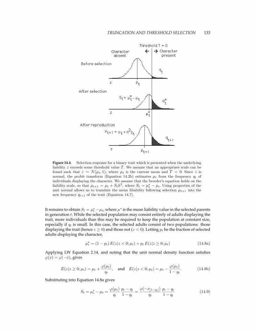
Figure 14.4. Selection response for a binary trait which is presented when the underlyingliability z exceeds some threshold value T . We assume that an appropriate scale can befound such that z ∼ N(µt, 1), where µt is the current mean and T = 0. Since z isnormal, the probit transform (Equation 14.2b) estimates µt from the frequency qt ofindividuals displaying the character. We assume that the breeder’s equation holds on theliability scale, so that µt+1 = µt + Sth

2, where St = µ∗t − µt. Using properties of theunit normal allows us to translate the mean libability following selection µt+1 into thenew frequency qt+1 of the trait (Equation 14.7).

It remains to obtain St = µ∗t −µt, where µ∗ is the mean liability value in the selected parentsin generation t. While the selected population may consist entirely of adults displaying thetrait, more individuals than this may be required to keep the population at constant size,especially if qt is small. In this case, the selected adults consist of two populations: thosedisplaying the trait (hence z ≥ 0) and those not (z < 0). Letting pt be the fraction of selectedadults displaying the character,

µ∗t = (1− pt)E(z|z < 0;µt) + ptE(z|z ≥ 0;µt) (14.8a)

Applying LW Equation 2.14, and noting that the unit normal density function satisfiesϕ(x) = ϕ(−x), gives

E(z|z ≥ 0;µt) = µt +ϕ(µt)qt

, and E(z|z < 0;µt) = µt −ϕ(µt)1− qt

. (14.8b)

Substituting into Equation 14.8a gives

St = µ∗t − µt =ϕ(µt)qt

pt − qt1− qt

=ϕ(−x[1−qt])

qt

pt − qt1− qt

(14.9)

2520151050

0.00

0.25

0.50

0.75

1.00

1.25

1.50

1.75

2.00

2.25

0

10

20

30

40

50

60

70

80

90

100

Generation

Sel

ectio

n di

ffere

ntia

l S

q, F

requ

ency

of c

hara

cter

134 CHAPTER 14

As expected, if pt > qt, then St > 0. Maximal selection occurs if only individuals displayingthe trait are saved ( pt = 1 ), in which case Equation 14.9 reduces to St = ϕ(µt)/qt.

Why we did not simply estimate µ∗t using x[1−q∗t ], i.e., using the frequency q∗ of the traitin the selected parents? The reason is that the distribution of z values in selected parentsis a weighted average of two truncated normal density functions (Equation 14.8a), and thisdistribution is not normal. However, we assume that normality is restored in the liabilitydistribution at the start of the next generation due to segregation plus the addition of theenvironmental value. We examine the validity of this assumption in Chapter 24.

Example 14.3. Consider a threshold trait whose liability has heritability h2 = 0.25(Example 14.4 and especially LW Chapter 25 discuss how h2 can be estimated). Whatis the expected response to selection if the initial frequency of individuals displayingthe character is 5% and selection is practiced by choosing only adults displaying thecharacter? As was calculated earlier, q0 = 0.05 implies µ0 = −1.645 (the mean liabilityis 1.65 standard deviations below the threshold). Only individuals displaying the traitare allowed to reproduce, giving (Equation 14.9) the resulting selection differential on theliability scale as

S0 = ϕ(−1.645)/0.05 ' 0.106/0.05 ' 2.062

Applying the breeder’s equation gives the new mean value of liability as

µ1 = µ0 + 0.25 · S0 = −1.645 + 0.25 · 2.062 = −1.129

Equation 14.7 translates this new mean into the fraction of the population now above thethreshold,

q1 = Pr(U ≥ −µ1) = Pr(U ≥ 1.129 ) = 0.129

Thus, after one generation of selection, the character frequency is expected to increasefrom 5% to 12.9%. Changes in q and S after further iterations (again where selectionoccurs by only allowing adults displaying the trait to reproduce) are plotted below, wheresolid circles denote qt, open squares denote St. Only six generations are required toincrease the frequency of the trait to 50% (µ = 0). Note that even though all selectedparents show the trait, the selection differential rapidly declines in a nonlinear fashion.

TRUNCATION AND THRESHOLD SELECTION 135

Example 14.4. The effectiveness of selection on wing morphs in females of the white-backed planthopper Sogatella furcifera was examined by Matsumura (1996). While thishemipterian is a serious rice pest in Japan, it is unable to overwinter. Rather, each yearit migrates from southern China to recolonize Japan. Females exhibit two wing morphs,males just one. Macropterous females are fully winged while brachypterous females havereduced wings and cannot fly. Further, increasing nymphal population density increasesthe frequency of macropterous females (leading to increased dispersal). Using three repli-cate experiments at each of three densities, Matsumura selected for increased macropteryin one replicate, decreased in another, and a control (no selection) in the third. For thereplicates with a density of one nymph, roughly 40-90 adults were scored, and 20 cho-sen to form the next generation. The resulting data for the first five generations in theup-selected line was as follows (Matsumura pers. comm.):

Generation q µ p S R1 0.224 -0.76 1.00 1.34 0.352 0.340 -0.41 0.80 0.75 0.543 0.551 0.13 1.00 0.72 0.334 0.675 0.45 1.00 0.53 -0.075 0.651 0.39 1.00 0.57 0.166 0.708 0.55

Here q is the frequency of macroptery before selection and p the frequency of macropteryin the selected parents. Translation from q into the mean liability µ follows from Equation14.6. The response (on the liability scale) to selection in generation one is

R(1) = µ2 − µ1 = −x[1−0.340] − (−x[1−0.224]) = −0.41− (−0.76) = 0.35

Likewise, the total response was

µ6 − µ1 = 0.55− (−0.76) = 1.31

Selection differentials were calculated from q and p using Equation 14.9. For example, forgeneration two,

S2 =ϕ(µ2)q2

p2 − q2

1− q2=ϕ(−0.41)

0.34(0.80− 0.34)

1− 0.34= 0.75

The total selection differential is∑i Si = 3.91. One key summary statistic for any

selection experiment is the realized heritability, the ratio of response to selection differential.As detailed in Chapter 18, there are several ways to compute this for a multi-generationselection experiment. One simple estimate is the total response/total differential ratio,

h2 =∑Ri∑i Si

=1.313.91

= 0.33

giving an estimated heritability of the underlying liability for macroptery of around 30%.

One important feature about selection on threshold traits is that response is not neces-sarily symmetric — a selected 5% increase in the trait may not yield the same response asa selected 5% decrease. The reason for this is that the mapping between phenotypes andtheir underlying liability is highly non-linear. Even though the parent-offspring regression

136 CHAPTER 14

on the liability scale is assumed to be linear (and hence liability response is symmetric), theparent-offspring regression on the phenotypic level is not linear, resulting in an asymmetricresponse.

Direct Selection on the Threshold T

It is biologically quite reasonable to imagine that there is variation in T itself (Hazel et al.1990). Suppose the trait of interest appears when the size of an organism exceeds some criti-cal value, which itself varies over individuals, with certain genotypes and/or environmentslowering the value of T , allowing individuals with a lower liability score to display the trait.Decomposing both the liability and threshold in terms of genetic and environmental factors,z = gz + ez and T = gT + eT . The trait appears when z ≥ T , or

gz + ez − (gT + eT ) = (gz − gT ) + (ez − eT ) = g + e ≥ 0

Thus, even though both the liability and threshold values are variable, we can simply con-sider a single new risk liability, the difference between the liability and threshold values,and the analysis proceeds as above. If interest is simply on presence/absence of the binarytrait, it does not matter as to whether the liability or threshold, or both, show variation.However, as Example 14.4 (below) shows, there are situations where we can directly mea-sure the threshold value itself, in which case we can directly measure the heritability of thethreshold level by a selection experiment.

The Logistic Regression Model for Binary Traits

The threshold approach offers one model for mapping an underlying continuous liabilityz into a discrete character space y (which is either zero or one, corresponding to trait ab-sence/presence). This is a deterministic model, with all individuals with z ≥ T displayingthe trait (y = 1), while all those with z < T do not (y = 0). A potentially more realisticmodel is that trait presence is stochastic, with the underlying liability z mapping into aprobability of displaying the trait, e.g., p(z) = Prob(y = 1 | z). Under the threshold model,this probability is one for z ≥ T , and zero otherwise. From a biological standpoint, oneimagines that p(z) is a monotonically increasing function of z, approaching zero for lowvalues and one for high values. One reasonable candidate that satisfies these requirementsis the logistic function,

`(z) =1

1 + exp(−z) (14.10a)

with `(z) ' 0 for z ¿ −1, ' 1 for z À 1, and `(0) = 1/2. A more general version is

`[α (z −m)] =1

1 + exp[−α (z −m)](14.10b)

which has value 0.5 at z = m and a scaling factor α that sets the abruptness of the transitionfrom low to high probability (Figure 14.5). The larger α, the more abrupt the transition,approaching the threshold model for sufficiently large α. Equation 14.10b is often called alogistic regression.

The logistic regression and threshold models are essentially identical. To see this, recallthat the threshold model very easily extends to the case where T varies over individuals.In such cases, if the liability value of an individual is z, the trait will only be displayed ifT ≤ z. Now consider the logistic regression model where p(z) denotes the probability thatan individual with liability value z displays the trait. One source of this stochasticity couldsimply be population variation in T , so that p(z) can be viewed as the cumulative distribution

0-1-2-3 321

α = 1

α = 5

α = 10

Liability score z

Pro

babi

lity

of th

e tr

ait

0

1

0.5

TRUNCATION AND THRESHOLD SELECTION 137

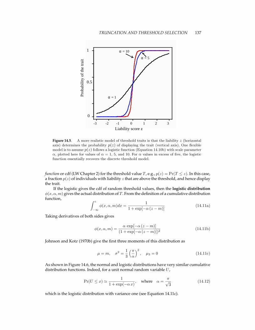
Figure 14.5. A more realistic model of threshold traits is that the liability z (horizontalaxis) determines the probability p(z) of displaying the trait (vertical axis). One flexiblemodel is to assume p(z) follows a logistic function (Equation 14.10b) with scale parameterα, plotted here for values of α = 1, 5, and 10. For α values in excess of five, the logisticfunction essentially recovers the discrete threshold model.

function or cdf (LW Chapter 2) for the threshold value T , e.g., p(z) = Pr(T ≤ z). In this case,a fraction p(z) of individuals with liability z that are above the threshold, and hence displaythe trait.

If the logistic gives the cdf of random threshold values, then the logistic distributionφ(x, α,m) gives the actual distribution ofT . From the definition of a cumulative distributionfunction, ∫ z

−∞φ(x, α,m)dx =

11 + exp[−α (z −m)]

(14.11a)

Taking derivatives of both sides gives

φ(x, α,m) =α exp[−α (z −m)]

(1 + exp[−α (z −m)])2(14.11b)

Johnson and Kotz (1970b) give the first three moments of this distribution as

µ = m, σ2 =13

(πα

)2

, µ3 = 0 (14.11c)

As shown in Figure 14.6, the normal and logistic distributions have very similar cumulativedistribution functions. Indeed, for a unit normal random variable U ,

Pr(U ≤ x) ' 11 + exp(−αx)

, where α =π√3

(14.12)

which is the logistic distribution with variance one (see Equation 14.11c).

138 CHAPTER 14

Figure 14.6. A compairson of the unit normal and unit logistic (µ = 0, σ2 = 1) dis-tributions, with the horizontal axis the value of z. Left: Probability density functions:the logistic is more peaked, with positive kutosis. Right: The cumulative distributionfunctions are very similar.

Thus, we have two approaches for mapping liability values into binary traits: the strictthreshold approach (a deterministic mapping of liability into the discrete trait) or the logisticregression approach (a stochastic mapping translating a liability value into a probability ofobserving the trait). Given the very close connection between the threshold and logisticregression models, for most purposes the simple threshold model is a reasonable approach,even if the underlying mapping is stochastic, and as illustrated above can easily be used topredict selection response.

One setting where the logistic regression is more appropriate is in the actual analysisof the behavior of the thresehold when one either knows the liability value or has at least astrong proxy (such as size).

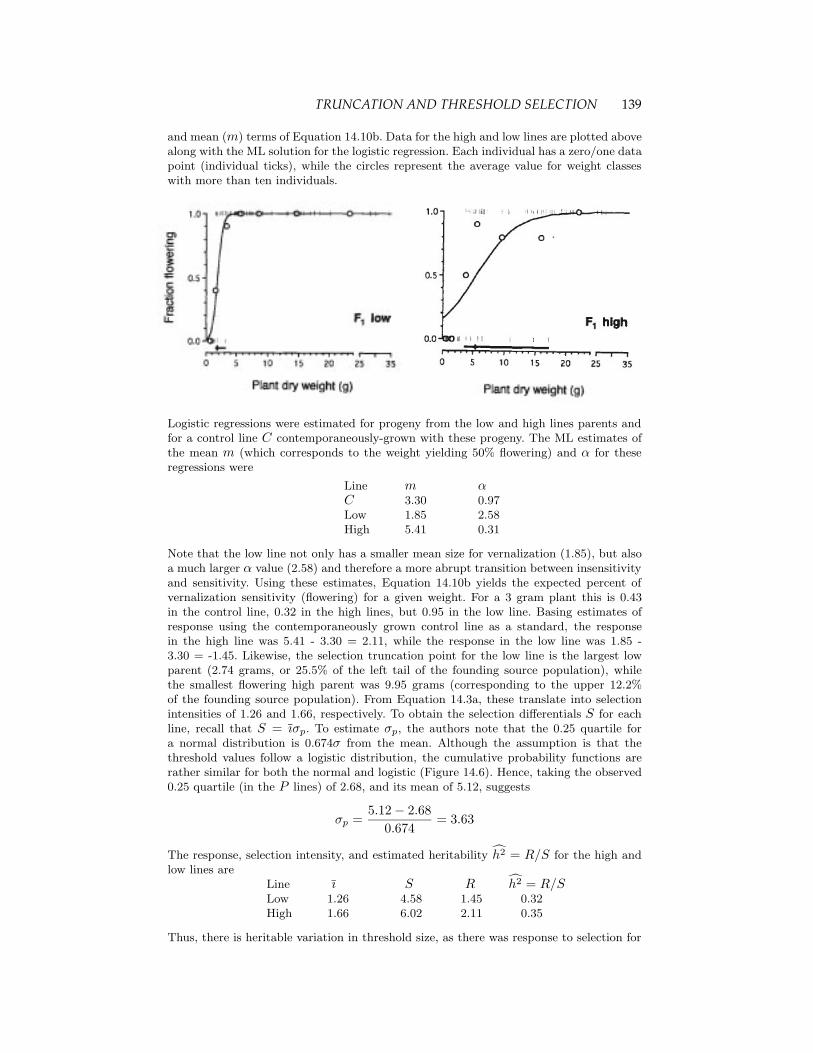
Example 14.5. An interesting analysis of selection on a threshold trait using logisticregressions was given by Wesselingh and de Jong (1995), who studied the connectionbetween plant size and flowering in hound’s-tongue (Cynoglossum officinale). This speciesis a facultative biennial, which means that, like an annual plant, it flowers only once, butunlike an annual, it may live several years before flowering. This represents a trade-offbetween the risk of survival over several years versus a larger seed set from a larger size atflowering. For Cynoglossum it has been shown that vernalization (cold treatment) followedby an appropriate photoperiod is required for flowering. However, unless plants are at (orabove) a certain threshold size, they are unresponsive to vernalization and hence growwithout flowering through the next growing cycle. The authors were interested in thethreshold size that triggers the binary trait (vernalization sensitivity), and in particularwhether this size is both variable and heritable. To examine this, they grew plants fordifferent number of days (ranging from 31 to 86) to generate individuals of different sizesbefore vernalization treatment. This generated two selection groups: the smallest plantsthat flowered following vernalization where chosen as the low-line parents, while thoseplants that did not respond to the first vernalization treatment were allowed to grow asecond cycle and these were chosen as the parents for the high lines. As plotted below,threshold values for resulting F1 offspring from intercrosses within each set of selectedparents were examined.

The data available to the authors were 0/1 (insensitive/sensitive to vernalization) valuesas a function of size. To estimate the distribution of threshold sizes, they performed alogistic regression on these data, using maximum likelihood (LW Appendix 4) to fit the α

TRUNCATION AND THRESHOLD SELECTION 139

and mean (m) terms of Equation 14.10b. Data for the high and low lines are plotted abovealong with the ML solution for the logistic regression. Each individual has a zero/one datapoint (individual ticks), while the circles represent the average value for weight classeswith more than ten individuals.

Logistic regressions were estimated for progeny from the low and high lines parents andfor a control line C contemporaneously-grown with these progeny. The ML estimates ofthe mean m (which corresponds to the weight yielding 50% flowering) and α for theseregressions were

Line m αC 3.30 0.97Low 1.85 2.58High 5.41 0.31

Note that the low line not only has a smaller mean size for vernalization (1.85), but alsoa much larger α value (2.58) and therefore a more abrupt transition between insensitivityand sensitivity. Using these estimates, Equation 14.10b yields the expected percent ofvernalization sensitivity (flowering) for a given weight. For a 3 gram plant this is 0.43in the control line, 0.32 in the high lines, but 0.95 in the low line. Basing estimates ofresponse using the contemporaneously grown control line as a standard, the responsein the high line was 5.41 - 3.30 = 2.11, while the response in the low line was 1.85 -3.30 = -1.45. Likewise, the selection truncation point for the low line is the largest lowparent (2.74 grams, or 25.5% of the left tail of the founding source population), whilethe smallest flowering high parent was 9.95 grams (corresponding to the upper 12.2%of the founding source population). From Equation 14.3a, these translate into selectionintensities of 1.26 and 1.66, respectively. To obtain the selection differentials S for eachline, recall that S = ıσp. To estimate σp, the authors note that the 0.25 quartile fora normal distribution is 0.674σ from the mean. Although the assumption is that thethreshold values follow a logistic distribution, the cumulative probability functions arerather similar for both the normal and logistic (Figure 14.6). Hence, taking the observed0.25 quartile (in the P lines) of 2.68, and its mean of 5.12, suggests

σp =5.12− 2.68

0.674= 3.63

The response, selection intensity, and estimated heritability h2 = R/S for the high andlow lines are

Line ı S R h2 = R/SLow 1.26 4.58 1.45 0.32High 1.66 6.02 2.11 0.35

Thus, there is heritable variation in threshold size, as there was response to selection for

140 CHAPTER 14

both larger and smaller threshold sizes. Further, the estimated heritability (based on thesingle-generation response to selection) was around 0.3.

The other setting where the logistic regression model is used is for BLUP selection.Recall that animal breeders routinely use linear mixed models to obtain BLUP estimates ofbreeding values. The standard model for normally-distributed traits is to assume that anobservation for individual i can be written as

yi = µ+∑

βkxk,i +Ai + ei (14.13)

where the βk are fixed effects (such as adjustments for age and sex),Ai their breeding value,and the residual ei is normally distributed. In addition to yi, further information to estimateAi is borrowed from the y values of relatives through the relationship matrix A, with thoseindividuals with the largest estimated A values are chosen to form the next generation.Generalized linear mixed models extend Equation 14.13 to cases where (i) the expectedvalue of y conditioned on the variables of interest is not a linear function and (ii) the residualsabout this expected value are not necessarily normal. The basic structure of a generalizedlinear model is that the conditional expectation of y can be expressed as

E(y | z) = g(z) (14.14a)

for some montonic function g, with

g−1 [E(y | z)] = z = µ+∑

βkxk,i +Ai (14.14b)

The inverse g−1 is called the link function as it transforms the conditional expectation intoa linear model.

For binary data, a single value of y follows a Bernoulii distribution (y = 0 or 1) withsuccess parameter p(z) = Pr(y = 1 | z). Equation 14.14a becomes E(y |z) = p(z), so thatg(z) is given by `(z), where the simple logistic (Equation 14.10a) is used as one can alwayswork on a scale with m = 0, α = 1. The corresponding link function (Equation 14.14b), theinverse of the logistic function, is given by the logit function L(p),

L(p) = ln(

p

1− p

)(14.15a)

which is the log of the odds ratio (probability of the trait divided by probability that thetrait is absent). If `(z) = p, then L(p) = z, so that a logit-transformed p value recovers theliability value,

L(p|z) = z = µ+∑

βkxk,i +Ai (14.15b)

Under this framework, BLUP selection for individuals with the highest breeding values fora binary trait proceeds by taking the 0/1 binary data from a set of individuals (along withother fixed, and possibly random, effects of interest) and using either maximum likelihoodor bayesian approaches to estimate the breeding values (Foulley et al. 1983, Foulley 1992,Vazques et al. 2009). This approach can be extended to k ≥ 2 thresholds in the mapping ofliability into different character states (Korsgaard et al. 2002).

RESPONSE WITH DISCRETE TRAITS: POISSON-DISTRIBUTED CHARACTERS

TRUNCATION AND THRESHOLD SELECTION 141

Many discrete characters with multiple states, such as number of leaves on a tree, can betreated as a continuous trait with little error. However, what about a discrete trait with arather compact distribution? A common example would be number of offspring, such as theclutch size of a bird, which may range from (say) 0 to 10 eggs in our observed sample witha mean of (say) four. This discreteness is of special concern when the trait has a significantprobability mass at a particular value (especially zero), as often happens with offspringnumber.

A natural way to model such traits is to use the Poisson distribution, where the prob-ability of observing a character state of k is given by

Pr(y = k) = e−λλk

k!(14.16)

where λ = E(y) is the expected value of the trait. Motivated by the above treatment ofbinary traits, one might imagine that on some appropriate scale the mean value λ is akin tothe liability of an individual (we will define this a bit more precisely below). In particular,we can take

λ = exp(z) (14.17a)

ensuring for all z that λ > 0 and hence a proper expectation for a Poisson. In the context ofgeneralized linear models, g(z) = exp(z) so that the link function g−1(z) is just ln(z), with

ln(λ) = z = µ+A+ e (14.17b)

This is called a log-linear model, as the log of the distribution parameter λ is a linearfunction of the variables of interest (in particular, the breeding value). On this log scale,both the breeding and environmental values are assumed to be normal with mean zero andvariances σ2

A and σ2e . As with binary traits, BLUP selection occurs using this generalized

linear model framework to estimate the Ai values (Foulley 1993, Korsgaard et al. 2002,Vazques et al. 2009). Other models are also possible, such as a zero-inflated Poisson, whichhas extra probablity mass at zero relative to a standard Poisson (Rodrigues-Motta et al.2007).

Under the log-linear model, the liability z of an individual determines λ = exp(z) andthen a realization is drawn from a Poisson(λ) to give their observed trait value. The resultingmean trait value in a population becomes

E(y) = E(λ) = E[exp(z)]= E[ exp(µ) · exp(A) · exp(e) ]= exp(µ) · E[ exp(A) ] · E[ exp(e) ] (14.18)

where the last step follows since (by construction) A and e are uncorrelated, while µ is aconstant. To compute these expectations, recall that the expression E(etx) is the moment-generating function of the random variable x. For a normal (Johnson and Kotz 1970a),

E(etx) = exp(µt+

σ2

2t

)(14.19a)

For a normal random variable x with mean zero and variance σ2, setting t = 1 gives

E [exp(x) ] = exp(σ2

2

)(14.19b)

142 CHAPTER 14

Substituting into Equation 14.18 shows that the expected mean trait value is a function ofboth the mean µ and variance σ2

z of the underlying liability value,

E(y) = exp(µ) · exp(σ2A + σ2

e

2

)= exp(µ) · exp(σ2

z/2) (14.20a)

One might initially expect that ifA is the breeding value for liability, then its mean phenotypewould simply be exp(µ+A). However, Equation 14.20a shows that

E(y |A) = exp(µ+A) · exp(σ2e/2), (14.20b)

which reflects how variation about the expected value maps into phenotypic variation.Following a single generation of selection, the distribution of liability values has the

approximately the same variance, but now the mean is shifted to µ + h2S (where S is theselection differential on the liability scale). The response on the phenotypic scale becomes

R = E(yt+1)− E(yt)=(exp(µ+ h2S)− exp(µ)

)· exp(σ2

z/2)

=(exp(h2S)− 1

)· exp(µ) · exp(σ2

z/2)

=(exp(h2S)− 1

)· E(yt) (14.21)

Notice, as was the case for selection on a binary trait, that the response is not symmetric.An S of +δ does not give the same increment of response as an S of −δ.

TRUNCATION AND THRESHOLD SELECTION 143

Literature Cited

Bulmer, M. G. 1980. The mathematical theory of quantitative genetics. Oxford Univ. Press, NY. [14]

Burrows, P. M. 1972. Expected selection differentials for directional selection. Biomet. 28: 1091–1100.[14]

Burrows, P. M. 1975. Variance of selection differentials in normal samples. Biometrics 31: 125–133.[14]

Crow, J. F., and M. Kimura. 1979. Efficiency of truncation selection. Proc. Natl. Acad. Sci. USA 76:396–299. [14]

David, F. N. 1981. Order statistics, 2nd Ed. Wiley, New York. [14]

Foulley, J. L. 1992. Prediction of selection response from threshold dichotomous traits. Genetics 132:1187–1194. [14]

Foulley, J. L. 1993. Prediction of selection response for Poisson distributed traits. Genet. Sel. Evol25: 297–303. [14]

Foulley, J. L., D. Gianola, and R. Thompson. 1983. Prediction of genetic merit from data onbinary and quantitative variates with an application to calving difficulty, birth weight, andpelvic opening. Genet. Sel. Evol 15: 401–424. [14]

Harter, H. L. 1961. Expected values of normal order statistics. Biometrika 48: 151–166. [14]

Harter, H. L. 1970a. Order statistics and their use in testing and estimation. Volume 1: Tests based onrange and studentized range of samples from a normal population. U. S. Government Printing Office,Washington, D. C. [14]

Harter, H. L. 1970b. Order statistics and their use in testing and estimation. Volume 2: Estimates based onorder statistics of samples from various populations. U. S. Government Printing Office, Washington,D. C. [14]

Hazel, W. N. R. Smock, and M. D. Johnson. 1990. A polygenic model for the evolution and main-tenance of conditional strategies. Proceed. Royal Society London B 242: 181–187. [14]

Hill, W. G. 1976. Order statistics of correlated variables and implications in genetic selection pro-grammes. Biometrics 32: 889–902. [14]

Hill, W. G. 1977c. Order statistics of correlated variables and implications in genetic selectionprogrammes. II. Response to selection Biometrics 33: 703–712. [14]

Johnson, N. L., and S. Kotz. 1970a. Continuous univariate distributions – 1. John Wiley & Sons, NY.[14]

Johnson, N. L., and S. Kotz. 1970b. Continuous univariate distributions – 2. John Wiley & Sons, NY.[14]

Kendall, M., and A. Stuart. 1977. The advanced theory of statistics. Vol. 1. Distribution theory. 4th Ed.Macmillan, NY. [14]

Kimura, M., and J. F. Crow. 1978. Effect of overall phenotypic selection on genetic change atindividual loci. Prod. Natl. Acad. Sci. USA 75: 6168–6171. [14]

Korsgaard, I. R., A. H. Andersen, and J. Jensen. 2002. Prediction error variance and expectedresponse to selection, when selection is based on the best predictor – for Gaussian and thresholdcharacters, traits following a Poisson mixed model and survival traits. Genet. Sel. Evol 34: 307–333. [14]

Lande, R. 1978. Evolutionary mechanisms of limb loss in tetrapods. Evolution 32: 73–92. [14]

Lindgren, D. and J.-E. Nilsson 1985. Calculations concerning selection intensity. Report 5, SwedishUniversity of Agricultural Sciences, Ulmea. [14]

Matsumura, M. 1996. Genetic analysis of a threshold trait: density-dependent wing dimorphismin Sogatella fucifera (Horvath) (Hemiptera: Delphacidae), the whitebacked planthopper. Heredity76: 229 – 237. [14]

Montaldo, H. H. 1997. Optimization of selection response using artifical insemination and newreproductive technologies in diary cattle. Thesis, Department of Animal Science, University ofNebraska. [14]

144 CHAPTER 14

Nordskog, A. W., and A. J. Wyatt. 1952. Genetic improvement as related to size of breedingoperations. Poulty Sci 31: 1062–1066. [14]

Rawlings, J. O. 1976. Order statistics for a special class of unequally correlated multinormal variates.Biometrics 32: 875–887. [14]

Rodrigues-Motta, M., D. Gianola, B. Heringstad, G. J. M. Roza, and Y. M. Chang. 2007. A zero-inflated Poisson model for genetic analysis of number of mastitis cases in Norwegian Red cows.J. Dairy Sci. 90: 5306–5315. [14]

Roff, D. A. 1996. The evolution of threshold traits in animals. Quarterly Review of Biology 71: 3–35.[14]

Sarhan, A. E. and B. G. Greenberg. 1962. Contributions to order statistics. Wiley, New York. [14]

Saxton, A. M. 1988. Further approximations for selection intensity. Theor. Appl. Genet 76: 465–466.[14]

Simmonds, N. W. 1977. Approximations for i, intensity of selection. Heredity 38: 413–414. [14]

Smith, C. 1969. Optimum selection procedures in animal breeding. Anim. Prod. 11: 433–442. [14]

Tukey, J. W. 1962. The future of data analysis. Annals of Math.l Stats 33: 1-67. [14]

Vazquez, A. I., D. Gianola, D. Bates, K. A. Weigel, and B. Heringstad. 2009. Assessment of Poisson,logit, and linear models for genetic analysis of clinical mastitis in Norwegian Red cows. J. DairySci. 92: 739–748. [14]

Wesselingh, R. A., and T. J. De Jong. 1995. Bidirectional selection on threshold size for floweringin Cynoglossum officinale (hound’s-tough). Heredity 74: 415–424. [14]