Chapter 12 - Unleashing Capitalism
22
CHAPTER 12 by Daniel S. Sutter and Andres Bello CONSTITUTIONALLY CONSTRAIN GOVERNMENT TO UNLEASH CAPITALISM 225
Transcript of Chapter 12 - Unleashing Capitalism
16
REFERENCES
Autor, David H. and Mark G Duggan. 2002. The Rise in Disability Recipiency and the
Decline in Unemployment. Chestnut Hill: center for Retirement Research at Boston College.
Benitez-Silva, Hugo, Moshe Buchinsky, and John Rust. 2004. How Large are the Classification Errors in the Social Security Disability Award Process? NBER Working
Paper No. 10219. Cambridge: National Bureau of Economic Research. Bureau of Economic Analysis, U.S. Department of Commerce. 2009. Regional Economic
Information System [electronic file]. Washington, DC: U.S. Department of Commerce. Online: http://www.bea.gov/regional/index.htm (accessed: August 20, 2009).
Bureau of Labor Statistics, U.S. Department of Labor. 2009. Glossary [electronic file]. Washington, DC: U.S. Department of Labor. Online: http://www.bls.gove/bls/ glossary.htm (accessed: August 20, 2009).
Bureau of Labor Statistics, U.S. Department of Labor. 2009. Regional Data [electronic file]. Washington DC: U.S. Department of Labor. Online http://www.bea.gov/regional/ index.htm (accessed: August 20, 2009).
National Association of Child Care Resource and Referral Agencies. 2006. Breaking the Piggy Bank-Parents and the High Price of Child Care Report, Appendix A [electronic file] Arlington, VA. Online: http://www.naccrra.org/ (accessed: August 20, 2009).
Low Income Working Families Project. 2008. Net Income Calculator [electronic file]. Washington DC: Urban Institute. Online: http://www.urban.org/center/lwf/index.cfm (accessed: August 10, 2009)
Social Security Administration. 2009. Supplemental Security Income [electronic file]. Washington DC: U.S. Social Security Administration. Online: http://www.ssa.gov/ notices/supplemental-security-income/ (accessed: August 20, 2009).
South Carolina Department of Social Services. 2009. Family Independence [electronic file]. Columbia SC. Online: http://dss.sc.gov/content/customers/finance/fi.aspx (accessed August 20, 2009). U.S. Census Bureau. 2009. Historical Tables of Poverty: 1980-2007 [electronic file]. Washington, DC: U.S. Census Bureau, Current Population Survey, Annual Social and Economic Supplements. Online: http://www.census.gove/hhes/poverty/histpov/ hstpov21.html (accessed: August 20, 2009).
U.S. Department of Health and Human Services. 2009. Administration for Children & Families: Services [electronic file]. Washington, D.C: U.S. Department of Health and Human Services. Online: http://www.acf.hhs.gov/acf_services.html#walia (accessed: August 20, 2009).
U.S. Department of Health and Human Services. 2009. Administration for Children & Families: TANF Work Participation Rates [electronic file]. Washington, D.C: U.S. Department of Health and Human Services. Online: http://www.acf.hhs.gov/programs /ofa/particip/indexparticp.html (accessed: August 20, 2009).
C H A P T E R 1 2
by Daniel S. Sutter and Andres Bello
C O N S T I T U T I O N A L L Y C O N S T R A I N
G O V E R N M E N T T O
U N L E A S H C A P I T A L I S M
UNLEASHING CAPITALISM 18
manufacturing property tax in the country. In Figure 5.8 we present the effective property tax rates data for Southeastern states, for comparison. The ranks given for the states are out of all 50 states. The ‘net tax’ and ‘effective tax rate’ are calculated based on property valued at $25 million ($12.5 million in machinery and equipment, $12.5 million in inventories, and $2.5 million in fixtures). Notice that South Carolina’s effective tax rate on industrial property is over 7.8 times higher than the most industry-friendly state, Delaware. (Delaware is listed in the figure because it is the lowest-tax state.)
Figure 5.8: Industrial Property Taxes in Southeastern states*, 2007 State Rank (of 50) Net Tax Effective Tax Rate
South Carolina 1 $1,864,900 3.73%
Mississippi 4 $1,291,050 2.58%
Texas 6 $1,264,358 2.53%
Tennessee 10 $1,033,544 2.07%
West Virginia 14 $833,234 1.67%
Louisiana 17 $783,407 1.57%
Georgia 20 $760,381 1.52%
Florida 24 $677,683 1.36%
Alabama 35 $533,776 1.11%
North Carolina 37 $491,071 0.98%
Kentucky 47 $327,100 0.65%
Virginia 49 $241,498 0.48%
Delaware 50 $238,840 0.48%
Source: National Association of Manufacturers (2009) * Taxes measured in the states’ largest city only.
Importantly, South Carolina’s effective tax rate is almost 2.5 times greater than Georgia’s tax, and almost 4 times greater than North Carolina’s. This puts South Carolina at a serious disadvantage, in terms of its ability to attract and keep industry. Since South Carolina has the highest tax in the country on industrial property, it should be no surprise that it has one of the lowest per capita incomes and economic growth rates in the country. Although it is probably not critical that South Carolina set its tax rate to the lowest in the country, it should definitely make it at least competitive for the Southeast. Since Georgia’s rate is effectively 1.52 percent and North Carolina’s is just under 1 percent, a rate at around 1 percent might be sufficient to attract more industry. Working to reduce the various taxes applied to industry would seriously improve the state’s competitiveness. Such a significant reduction in taxes on industrial property would obviously lead to a reduction in tax revenues on industrial property, at least initially. However, the overall revenue may in fact increase once the growth rate in the state begins to pick up and more industry moves into the state. Furthermore, if the official tax rates are lowered, then the state
225CHAPTER 5: SPECIFIC TAX REFORMS
13
Presumably the original intent of imposing a tax rate schedule with graduated marginal tax rates was to make the income tax progressive. However, what progressivity exists in the state’s income tax structure is due to the zero tax on the first $2,630 of income, and because of the graduated marginal tax rates. However, since the marginal tax rate increases over such small steps in income, as shown in Figure 5.5, most of the progressivity occurs at lower income levels, not higher levels of income. At higher income levels, the average tax rate hardly increases at all. This nature of the current tax is directly contradictory to the goal of progressivity. So although on the surface it appears that the tax satisfies the vertical equity condition, it really does this only at the lower income levels reducing the wealth of these lowest income taxpayers, not the intended consequence.
Figure 5.5: South Carolina income tax: Current tax rates compared to inflation-indexed rates, 2009
Current Income Tax
Rates/Brackets
Income Tax Rates/Brackets if 1959 Tax Schedule was Inflation Adjusted to
2009
Taxable Income Tax
Amount Average Tax Rate
Tax Amount
Average Tax Rate
$5,000 $71 1.42% $125 2.5%
$10,000 $290 2.90% $250 2.5%
$15,000 $604 4.03% $377 2.51%
$20,000 $954 4.77% $527 2.63%
$30,000 $1,654 5.51% $834 2.78%
$50,000 $3,054 6.10% $1,695 3.39%
$75,000 $4,804 6.41% $3,127 4.17%
$100,000 $6,554 6.56% $4,877 4.88%
$150,000 $10,054 6.70% $8,377 5.58%
$200,000 $13,554 6.77% $11,877 5.94%
Figure 5.5 also shows what the average tax rates are for various incomes and taxes
under the current tax system in South Carolina. In the right columns it also shows what the taxes and average tax rates would be if the 1959 tax tables were indexed for inflation. The figure clearly shows that the 1959 indexed tax rate structure is more uniformly progressive, especially at higher levels of incomes. It keeps tax rates extremely low for the lowest income individuals in the state. Figure 5.5 also shows that the current tax system charges all income groups more in taxes than an indexed rate schedule. The only exception is the $5,000 income earner in the table. As South Carolina income taxes continue to climb while the tax brackets remain stagnant, the state becomes a relatively high-tax state. This has a negative impact on

3
12
CONSTITUTIONALLY CONSTRAIN
GOVERNMENT TO UNLEASH CAPITALISM
Daniel Sutter and Andres Bello
INTRODUCTION
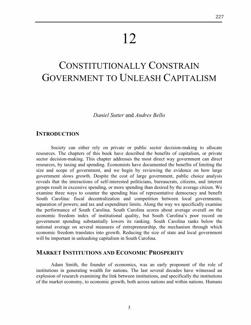
Society can either rely on private or public sector decision-making to allocate
resources. The chapters of this book have described the benefits of capitalism, or private sector decision-making. This chapter addresses the most direct way government can direct resources, by taxing and spending. Economists have documented the benefits of limiting the size and scope of government, and we begin by reviewing the evidence on how large government slows growth. Despite the cost of large government, public choice analysis reveals that the interactions of self-interested politicians, bureaucrats, citizens, and interest groups result in excessive spending, or more spending than desired by the average citizen. We examine three ways to counter the spending bias of representative democracy and benefit South Carolina: fiscal decentralization and competition between local governments; separation of powers; and tax and expenditure limits. Along the way we specifically examine the performance of South Carolina. South Carolina scores about average overall on the economic freedom index of institutional quality, but South Carolina’s poor record on government spending substantially lowers its ranking. South Carolina ranks below the national average on several measures of entrepreneurship, the mechanism through which economic freedom translates into growth. Reducing the size of state and local government will be important in unleashing capitalism in South Carolina.
MARKET INSTITUTIONS AND ECONOMIC PROSPERITY Adam Smith, the founder of economics, was an early proponent of the role of institutions in generating wealth for nations. The last several decades have witnessed an explosion of research examining the link between institutions, and specifically the institutions of the market economy, to economic growth, both across nations and within nations. Humans
UNLEASHING CAPITALISM 18
manufacturing property tax in the country. In Figure 5.8 we present the effective property tax rates data for Southeastern states, for comparison. The ranks given for the states are out of all 50 states. The ‘net tax’ and ‘effective tax rate’ are calculated based on property valued at $25 million ($12.5 million in machinery and equipment, $12.5 million in inventories, and $2.5 million in fixtures). Notice that South Carolina’s effective tax rate on industrial property is over 7.8 times higher than the most industry-friendly state, Delaware. (Delaware is listed in the figure because it is the lowest-tax state.)
Figure 5.8: Industrial Property Taxes in Southeastern states*, 2007 State Rank (of 50) Net Tax Effective Tax Rate
South Carolina 1 $1,864,900 3.73%
Mississippi 4 $1,291,050 2.58%
Texas 6 $1,264,358 2.53%
Tennessee 10 $1,033,544 2.07%
West Virginia 14 $833,234 1.67%
Louisiana 17 $783,407 1.57%
Georgia 20 $760,381 1.52%
Florida 24 $677,683 1.36%
Alabama 35 $533,776 1.11%
North Carolina 37 $491,071 0.98%
Kentucky 47 $327,100 0.65%
Virginia 49 $241,498 0.48%
Delaware 50 $238,840 0.48%
Source: National Association of Manufacturers (2009) * Taxes measured in the states’ largest city only.
Importantly, South Carolina’s effective tax rate is almost 2.5 times greater than Georgia’s tax, and almost 4 times greater than North Carolina’s. This puts South Carolina at a serious disadvantage, in terms of its ability to attract and keep industry. Since South Carolina has the highest tax in the country on industrial property, it should be no surprise that it has one of the lowest per capita incomes and economic growth rates in the country. Although it is probably not critical that South Carolina set its tax rate to the lowest in the country, it should definitely make it at least competitive for the Southeast. Since Georgia’s rate is effectively 1.52 percent and North Carolina’s is just under 1 percent, a rate at around 1 percent might be sufficient to attract more industry. Working to reduce the various taxes applied to industry would seriously improve the state’s competitiveness. Such a significant reduction in taxes on industrial property would obviously lead to a reduction in tax revenues on industrial property, at least initially. However, the overall revenue may in fact increase once the growth rate in the state begins to pick up and more industry moves into the state. Furthermore, if the official tax rates are lowered, then the state
226 CHAPTER 5: SPECIFIC TAX REFORMS
13
Presumably the original intent of imposing a tax rate schedule with graduated marginal tax rates was to make the income tax progressive. However, what progressivity exists in the state’s income tax structure is due to the zero tax on the first $2,630 of income, and because of the graduated marginal tax rates. However, since the marginal tax rate increases over such small steps in income, as shown in Figure 5.5, most of the progressivity occurs at lower income levels, not higher levels of income. At higher income levels, the average tax rate hardly increases at all. This nature of the current tax is directly contradictory to the goal of progressivity. So although on the surface it appears that the tax satisfies the vertical equity condition, it really does this only at the lower income levels reducing the wealth of these lowest income taxpayers, not the intended consequence.
Figure 5.5: South Carolina income tax: Current tax rates compared to inflation-indexed rates, 2009
Current Income Tax
Rates/Brackets
Income Tax Rates/Brackets if 1959 Tax Schedule was Inflation Adjusted to
2009
Taxable Income Tax
Amount Average Tax Rate
Tax Amount
Average Tax Rate
$5,000 $71 1.42% $125 2.5%
$10,000 $290 2.90% $250 2.5%
$15,000 $604 4.03% $377 2.51%
$20,000 $954 4.77% $527 2.63%
$30,000 $1,654 5.51% $834 2.78%
$50,000 $3,054 6.10% $1,695 3.39%
$75,000 $4,804 6.41% $3,127 4.17%
$100,000 $6,554 6.56% $4,877 4.88%
$150,000 $10,054 6.70% $8,377 5.58%
$200,000 $13,554 6.77% $11,877 5.94%
Figure 5.5 also shows what the average tax rates are for various incomes and taxes
under the current tax system in South Carolina. In the right columns it also shows what the taxes and average tax rates would be if the 1959 tax tables were indexed for inflation. The figure clearly shows that the 1959 indexed tax rate structure is more uniformly progressive, especially at higher levels of incomes. It keeps tax rates extremely low for the lowest income individuals in the state. Figure 5.5 also shows that the current tax system charges all income groups more in taxes than an indexed rate schedule. The only exception is the $5,000 income earner in the table. As South Carolina income taxes continue to climb while the tax brackets remain stagnant, the state becomes a relatively high-tax state. This has a negative impact on
3
12
CONSTITUTIONALLY CONSTRAIN
GOVERNMENT TO UNLEASH CAPITALISM
Daniel Sutter and Andres Bello
INTRODUCTION
Society can either rely on private or public sector decision-making to allocate
resources. The chapters of this book have described the benefits of capitalism, or private sector decision-making. This chapter addresses the most direct way government can direct resources, by taxing and spending. Economists have documented the benefits of limiting the size and scope of government, and we begin by reviewing the evidence on how large government slows growth. Despite the cost of large government, public choice analysis reveals that the interactions of self-interested politicians, bureaucrats, citizens, and interest groups result in excessive spending, or more spending than desired by the average citizen. We examine three ways to counter the spending bias of representative democracy and benefit South Carolina: fiscal decentralization and competition between local governments; separation of powers; and tax and expenditure limits. Along the way we specifically examine the performance of South Carolina. South Carolina scores about average overall on the economic freedom index of institutional quality, but South Carolina’s poor record on government spending substantially lowers its ranking. South Carolina ranks below the national average on several measures of entrepreneurship, the mechanism through which economic freedom translates into growth. Reducing the size of state and local government will be important in unleashing capitalism in South Carolina.
MARKET INSTITUTIONS AND ECONOMIC PROSPERITY Adam Smith, the founder of economics, was an early proponent of the role of institutions in generating wealth for nations. The last several decades have witnessed an explosion of research examining the link between institutions, and specifically the institutions of the market economy, to economic growth, both across nations and within nations. Humans
UNLEASHING CAPITALISM 18
manufacturing property tax in the country. In Figure 5.8 we present the effective property tax rates data for Southeastern states, for comparison. The ranks given for the states are out of all 50 states. The ‘net tax’ and ‘effective tax rate’ are calculated based on property valued at $25 million ($12.5 million in machinery and equipment, $12.5 million in inventories, and $2.5 million in fixtures). Notice that South Carolina’s effective tax rate on industrial property is over 7.8 times higher than the most industry-friendly state, Delaware. (Delaware is listed in the figure because it is the lowest-tax state.)
Figure 5.8: Industrial Property Taxes in Southeastern states*, 2007 State Rank (of 50) Net Tax Effective Tax Rate
South Carolina 1 $1,864,900 3.73%
Mississippi 4 $1,291,050 2.58%
Texas 6 $1,264,358 2.53%
Tennessee 10 $1,033,544 2.07%
West Virginia 14 $833,234 1.67%
Louisiana 17 $783,407 1.57%
Georgia 20 $760,381 1.52%
Florida 24 $677,683 1.36%
Alabama 35 $533,776 1.11%
North Carolina 37 $491,071 0.98%
Kentucky 47 $327,100 0.65%
Virginia 49 $241,498 0.48%
Delaware 50 $238,840 0.48%
Source: National Association of Manufacturers (2009) * Taxes measured in the states’ largest city only.
Importantly, South Carolina’s effective tax rate is almost 2.5 times greater than Georgia’s tax, and almost 4 times greater than North Carolina’s. This puts South Carolina at a serious disadvantage, in terms of its ability to attract and keep industry. Since South Carolina has the highest tax in the country on industrial property, it should be no surprise that it has one of the lowest per capita incomes and economic growth rates in the country. Although it is probably not critical that South Carolina set its tax rate to the lowest in the country, it should definitely make it at least competitive for the Southeast. Since Georgia’s rate is effectively 1.52 percent and North Carolina’s is just under 1 percent, a rate at around 1 percent might be sufficient to attract more industry. Working to reduce the various taxes applied to industry would seriously improve the state’s competitiveness. Such a significant reduction in taxes on industrial property would obviously lead to a reduction in tax revenues on industrial property, at least initially. However, the overall revenue may in fact increase once the growth rate in the state begins to pick up and more industry moves into the state. Furthermore, if the official tax rates are lowered, then the state
227CHAPTER 5: SPECIFIC TAX REFORMS
13
Presumably the original intent of imposing a tax rate schedule with graduated marginal tax rates was to make the income tax progressive. However, what progressivity exists in the state’s income tax structure is due to the zero tax on the first $2,630 of income, and because of the graduated marginal tax rates. However, since the marginal tax rate increases over such small steps in income, as shown in Figure 5.5, most of the progressivity occurs at lower income levels, not higher levels of income. At higher income levels, the average tax rate hardly increases at all. This nature of the current tax is directly contradictory to the goal of progressivity. So although on the surface it appears that the tax satisfies the vertical equity condition, it really does this only at the lower income levels reducing the wealth of these lowest income taxpayers, not the intended consequence.
Figure 5.5: South Carolina income tax: Current tax rates compared to inflation-indexed rates, 2009
Current Income Tax
Rates/Brackets
Income Tax Rates/Brackets if 1959 Tax Schedule was Inflation Adjusted to
2009
Taxable Income Tax
Amount Average Tax Rate
Tax Amount
Average Tax Rate
$5,000 $71 1.42% $125 2.5%
$10,000 $290 2.90% $250 2.5%
$15,000 $604 4.03% $377 2.51%
$20,000 $954 4.77% $527 2.63%
$30,000 $1,654 5.51% $834 2.78%
$50,000 $3,054 6.10% $1,695 3.39%
$75,000 $4,804 6.41% $3,127 4.17%
$100,000 $6,554 6.56% $4,877 4.88%
$150,000 $10,054 6.70% $8,377 5.58%
$200,000 $13,554 6.77% $11,877 5.94%
Figure 5.5 also shows what the average tax rates are for various incomes and taxes
under the current tax system in South Carolina. In the right columns it also shows what the taxes and average tax rates would be if the 1959 tax tables were indexed for inflation. The figure clearly shows that the 1959 indexed tax rate structure is more uniformly progressive, especially at higher levels of incomes. It keeps tax rates extremely low for the lowest income individuals in the state. Figure 5.5 also shows that the current tax system charges all income groups more in taxes than an indexed rate schedule. The only exception is the $5,000 income earner in the table. As South Carolina income taxes continue to climb while the tax brackets remain stagnant, the state becomes a relatively high-tax state. This has a negative impact on
4
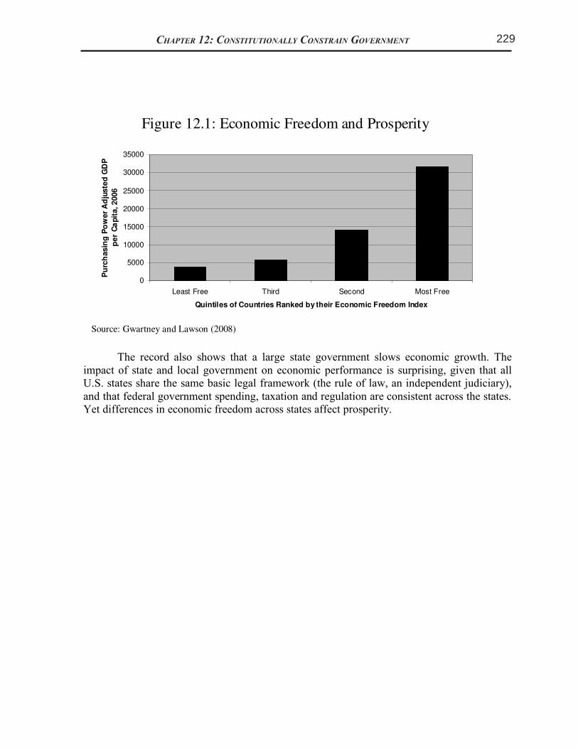
have an inherent tendency to improve the quality of their lives, and the institutions of a market economy harness this self-interest in service of others through the profit incentive. Much of the recent research on institutions and economic performance employs an index of economic freedom for more than 140 countries worldwide compiled by the Fraser Institute (Gwartney and Lawson 2008). The international economic freedom index measures the quality of institutions based on five component areas: the size of government, the legal system and protection of property rights, the quality of the money supply, freedom to engage in international trade, and economic regulation (e.g., of credit and labor markets). The index is a score from 0 to 10, with 10 representing a high level of economic freedom. The index allows comparisons between countries, or a way to classify countries as having more or less economic freedom. A market economy requires a legal infrastructure protecting property rights and the freedom to trade. Internationally, many weak or predatory governments fail to supply the basic framework for market exchange, with terrible consequences for human well-being, as illustrated by Figure 12.1. The figure reports Gross Domestic Product (GDP) per capita, a measure of the standard of living across nations, averaged across quintiles of countries as ranked by their economic freedom score, as reported by Gwartney and Lawson (2008). GDP per capita is nearly ten times higher in the top 25 percent of countries as ranked by economic freedom than in the bottom 25 percent of countries. These differences in standard of living did not occur over night, and can reflect the cumulative impact over decades of an environment hospitable to a market economy. The difference between the top and bottom quartiles of nations reflects the effect of the lack of protection of property and the rule of law. But GDP per capita is still more than double in the freest 25 percent of countries than in the second 25 percent, so even among nations where the rule of law is reasonably well established, limiting government spending and regulation is critical for growth and a high standard of living.1 Economic freedom does not merely lead to the pursuit of a narrow measure of the standard of living, or produce growth for some at the expense of poverty for others. Norton and Gwartney (2008) show that economic freedom reduces extreme poverty and improves a nation’s score on the United Nations’ Human Poverty Index.
1 Economists have extensively investigated the relationship between economic freedom and prosperity. For a
discussion of some of the findings of these studies, see Gwartney, Holcombe and Lawson (2004) and Lawson
(2007).
5
Figure 12.1: Economic Freedom and Prosperity
$0
$5,000
$10,000
$15,000
$20,000
$25,000
$30,000
$35,000
Least Free Third Second Most Free
Quintiles of Countries Ranked by their Economic Freedom Index
Purc
hasin
g
Pow
er
Adju
ste
d
GD
P
per
Capit
a,
20
06
Source: Gwartney and Lawson (2008)
The record also shows that a large state government slows economic growth. The impact of state and local government on economic performance is surprising, given that all U.S. states share the same basic legal framework (the rule of law, an independent judiciary), and that federal government spending, taxation and regulation are consistent across the states. Yet differences in economic freedom across states affect prosperity.
UNLEASHING CAPITALISM 18
manufacturing property tax in the country. In Figure 5.8 we present the effective property tax rates data for Southeastern states, for comparison. The ranks given for the states are out of all 50 states. The ‘net tax’ and ‘effective tax rate’ are calculated based on property valued at $25 million ($12.5 million in machinery and equipment, $12.5 million in inventories, and $2.5 million in fixtures). Notice that South Carolina’s effective tax rate on industrial property is over 7.8 times higher than the most industry-friendly state, Delaware. (Delaware is listed in the figure because it is the lowest-tax state.)
Figure 5.8: Industrial Property Taxes in Southeastern states*, 2007 State Rank (of 50) Net Tax Effective Tax Rate
South Carolina 1 $1,864,900 3.73%
Mississippi 4 $1,291,050 2.58%
Texas 6 $1,264,358 2.53%
Tennessee 10 $1,033,544 2.07%
West Virginia 14 $833,234 1.67%
Louisiana 17 $783,407 1.57%
Georgia 20 $760,381 1.52%
Florida 24 $677,683 1.36%
Alabama 35 $533,776 1.11%
North Carolina 37 $491,071 0.98%
Kentucky 47 $327,100 0.65%
Virginia 49 $241,498 0.48%
Delaware 50 $238,840 0.48%
Source: National Association of Manufacturers (2009) * Taxes measured in the states’ largest city only.
Importantly, South Carolina’s effective tax rate is almost 2.5 times greater than Georgia’s tax, and almost 4 times greater than North Carolina’s. This puts South Carolina at a serious disadvantage, in terms of its ability to attract and keep industry. Since South Carolina has the highest tax in the country on industrial property, it should be no surprise that it has one of the lowest per capita incomes and economic growth rates in the country. Although it is probably not critical that South Carolina set its tax rate to the lowest in the country, it should definitely make it at least competitive for the Southeast. Since Georgia’s rate is effectively 1.52 percent and North Carolina’s is just under 1 percent, a rate at around 1 percent might be sufficient to attract more industry. Working to reduce the various taxes applied to industry would seriously improve the state’s competitiveness. Such a significant reduction in taxes on industrial property would obviously lead to a reduction in tax revenues on industrial property, at least initially. However, the overall revenue may in fact increase once the growth rate in the state begins to pick up and more industry moves into the state. Furthermore, if the official tax rates are lowered, then the state
228 CHAPTER 5: SPECIFIC TAX REFORMS
13
Presumably the original intent of imposing a tax rate schedule with graduated marginal tax rates was to make the income tax progressive. However, what progressivity exists in the state’s income tax structure is due to the zero tax on the first $2,630 of income, and because of the graduated marginal tax rates. However, since the marginal tax rate increases over such small steps in income, as shown in Figure 5.5, most of the progressivity occurs at lower income levels, not higher levels of income. At higher income levels, the average tax rate hardly increases at all. This nature of the current tax is directly contradictory to the goal of progressivity. So although on the surface it appears that the tax satisfies the vertical equity condition, it really does this only at the lower income levels reducing the wealth of these lowest income taxpayers, not the intended consequence.
Figure 5.5: South Carolina income tax: Current tax rates compared to inflation-indexed rates, 2009
Current Income Tax
Rates/Brackets
Income Tax Rates/Brackets if 1959 Tax Schedule was Inflation Adjusted to
2009
Taxable Income Tax
Amount Average Tax Rate
Tax Amount
Average Tax Rate
$5,000 $71 1.42% $125 2.5%
$10,000 $290 2.90% $250 2.5%
$15,000 $604 4.03% $377 2.51%
$20,000 $954 4.77% $527 2.63%
$30,000 $1,654 5.51% $834 2.78%
$50,000 $3,054 6.10% $1,695 3.39%
$75,000 $4,804 6.41% $3,127 4.17%
$100,000 $6,554 6.56% $4,877 4.88%
$150,000 $10,054 6.70% $8,377 5.58%
$200,000 $13,554 6.77% $11,877 5.94%
Figure 5.5 also shows what the average tax rates are for various incomes and taxes
under the current tax system in South Carolina. In the right columns it also shows what the taxes and average tax rates would be if the 1959 tax tables were indexed for inflation. The figure clearly shows that the 1959 indexed tax rate structure is more uniformly progressive, especially at higher levels of incomes. It keeps tax rates extremely low for the lowest income individuals in the state. Figure 5.5 also shows that the current tax system charges all income groups more in taxes than an indexed rate schedule. The only exception is the $5,000 income earner in the table. As South Carolina income taxes continue to climb while the tax brackets remain stagnant, the state becomes a relatively high-tax state. This has a negative impact on
4
have an inherent tendency to improve the quality of their lives, and the institutions of a market economy harness this self-interest in service of others through the profit incentive. Much of the recent research on institutions and economic performance employs an index of economic freedom for more than 140 countries worldwide compiled by the Fraser Institute (Gwartney and Lawson 2008). The international economic freedom index measures the quality of institutions based on five component areas: the size of government, the legal system and protection of property rights, the quality of the money supply, freedom to engage in international trade, and economic regulation (e.g., of credit and labor markets). The index is a score from 0 to 10, with 10 representing a high level of economic freedom. The index allows comparisons between countries, or a way to classify countries as having more or less economic freedom. A market economy requires a legal infrastructure protecting property rights and the freedom to trade. Internationally, many weak or predatory governments fail to supply the basic framework for market exchange, with terrible consequences for human well-being, as illustrated by Figure 12.1. The figure reports Gross Domestic Product (GDP) per capita, a measure of the standard of living across nations, averaged across quintiles of countries as ranked by their economic freedom score, as reported by Gwartney and Lawson (2008). GDP per capita is nearly ten times higher in the top 25 percent of countries as ranked by economic freedom than in the bottom 25 percent of countries. These differences in standard of living did not occur over night, and can reflect the cumulative impact over decades of an environment hospitable to a market economy. The difference between the top and bottom quartiles of nations reflects the effect of the lack of protection of property and the rule of law. But GDP per capita is still more than double in the freest 25 percent of countries than in the second 25 percent, so even among nations where the rule of law is reasonably well established, limiting government spending and regulation is critical for growth and a high standard of living.1 Economic freedom does not merely lead to the pursuit of a narrow measure of the standard of living, or produce growth for some at the expense of poverty for others. Norton and Gwartney (2008) show that economic freedom reduces extreme poverty and improves a nation’s score on the United Nations’ Human Poverty Index.
1 Economists have extensively investigated the relationship between economic freedom and prosperity. For a
discussion of some of the findings of these studies, see Gwartney, Holcombe and Lawson (2004) and Lawson
(2007).
5
Figure 12.1: Economic Freedom and Prosperity
$0
$5,000
$10,000
$15,000
$20,000
$25,000
$30,000
$35,000
Least Free Third Second Most Free
Quintiles of Countries Ranked by their Economic Freedom Index
Purc
hasin
g
Pow
er
Adju
ste
d
GD
P
per
Capit
a,
20
06
Source: Gwartney and Lawson (2008)
The record also shows that a large state government slows economic growth. The impact of state and local government on economic performance is surprising, given that all U.S. states share the same basic legal framework (the rule of law, an independent judiciary), and that federal government spending, taxation and regulation are consistent across the states. Yet differences in economic freedom across states affect prosperity.
Chapter 12: Constitutionally Constrain government
Figure 12.1: Economic Freedom and Prosperity
0
5000
10000
15000
20000
25000
30000
35000
Least Free Third Second Most Free
Quintiles of Countries Ranked by their Economic Freedom Index
Pu
rch
asin
g P
ow
er
Ad
juste
d G
DP
pe
r C
ap
ita, 2
006
Source: Gwartney and Lawson (2008)
UNLEASHING CAPITALISM 18
manufacturing property tax in the country. In Figure 5.8 we present the effective property tax rates data for Southeastern states, for comparison. The ranks given for the states are out of all 50 states. The ‘net tax’ and ‘effective tax rate’ are calculated based on property valued at $25 million ($12.5 million in machinery and equipment, $12.5 million in inventories, and $2.5 million in fixtures). Notice that South Carolina’s effective tax rate on industrial property is over 7.8 times higher than the most industry-friendly state, Delaware. (Delaware is listed in the figure because it is the lowest-tax state.)
Figure 5.8: Industrial Property Taxes in Southeastern states*, 2007 State Rank (of 50) Net Tax Effective Tax Rate
South Carolina 1 $1,864,900 3.73%
Mississippi 4 $1,291,050 2.58%
Texas 6 $1,264,358 2.53%
Tennessee 10 $1,033,544 2.07%
West Virginia 14 $833,234 1.67%
Louisiana 17 $783,407 1.57%
Georgia 20 $760,381 1.52%
Florida 24 $677,683 1.36%
Alabama 35 $533,776 1.11%
North Carolina 37 $491,071 0.98%
Kentucky 47 $327,100 0.65%
Virginia 49 $241,498 0.48%
Delaware 50 $238,840 0.48%
Source: National Association of Manufacturers (2009) * Taxes measured in the states’ largest city only.
Importantly, South Carolina’s effective tax rate is almost 2.5 times greater than Georgia’s tax, and almost 4 times greater than North Carolina’s. This puts South Carolina at a serious disadvantage, in terms of its ability to attract and keep industry. Since South Carolina has the highest tax in the country on industrial property, it should be no surprise that it has one of the lowest per capita incomes and economic growth rates in the country. Although it is probably not critical that South Carolina set its tax rate to the lowest in the country, it should definitely make it at least competitive for the Southeast. Since Georgia’s rate is effectively 1.52 percent and North Carolina’s is just under 1 percent, a rate at around 1 percent might be sufficient to attract more industry. Working to reduce the various taxes applied to industry would seriously improve the state’s competitiveness. Such a significant reduction in taxes on industrial property would obviously lead to a reduction in tax revenues on industrial property, at least initially. However, the overall revenue may in fact increase once the growth rate in the state begins to pick up and more industry moves into the state. Furthermore, if the official tax rates are lowered, then the state
229CHAPTER 5: SPECIFIC TAX REFORMS
13
Presumably the original intent of imposing a tax rate schedule with graduated marginal tax rates was to make the income tax progressive. However, what progressivity exists in the state’s income tax structure is due to the zero tax on the first $2,630 of income, and because of the graduated marginal tax rates. However, since the marginal tax rate increases over such small steps in income, as shown in Figure 5.5, most of the progressivity occurs at lower income levels, not higher levels of income. At higher income levels, the average tax rate hardly increases at all. This nature of the current tax is directly contradictory to the goal of progressivity. So although on the surface it appears that the tax satisfies the vertical equity condition, it really does this only at the lower income levels reducing the wealth of these lowest income taxpayers, not the intended consequence.
Figure 5.5: South Carolina income tax: Current tax rates compared to inflation-indexed rates, 2009
Current Income Tax
Rates/Brackets
Income Tax Rates/Brackets if 1959 Tax Schedule was Inflation Adjusted to
2009
Taxable Income Tax
Amount Average Tax Rate
Tax Amount
Average Tax Rate
$5,000 $71 1.42% $125 2.5%
$10,000 $290 2.90% $250 2.5%
$15,000 $604 4.03% $377 2.51%
$20,000 $954 4.77% $527 2.63%
$30,000 $1,654 5.51% $834 2.78%
$50,000 $3,054 6.10% $1,695 3.39%
$75,000 $4,804 6.41% $3,127 4.17%
$100,000 $6,554 6.56% $4,877 4.88%
$150,000 $10,054 6.70% $8,377 5.58%
$200,000 $13,554 6.77% $11,877 5.94%
Figure 5.5 also shows what the average tax rates are for various incomes and taxes
under the current tax system in South Carolina. In the right columns it also shows what the taxes and average tax rates would be if the 1959 tax tables were indexed for inflation. The figure clearly shows that the 1959 indexed tax rate structure is more uniformly progressive, especially at higher levels of incomes. It keeps tax rates extremely low for the lowest income individuals in the state. Figure 5.5 also shows that the current tax system charges all income groups more in taxes than an indexed rate schedule. The only exception is the $5,000 income earner in the table. As South Carolina income taxes continue to climb while the tax brackets remain stagnant, the state becomes a relatively high-tax state. This has a negative impact on
6
Figure 12.2: Per Capita Income (2008) vs. Size of
State Government (1977)
20,000
25,000
30,000
35,000
40,000
45,000
50,000
55,000
60,000
4 6 8 10 12 14
State Spending as a Percent of Income (1977)
Per
Cap
tia P
erso
nal In
com
e (2
008)
Source: U.S. Census and Bureau of Economic Analysis
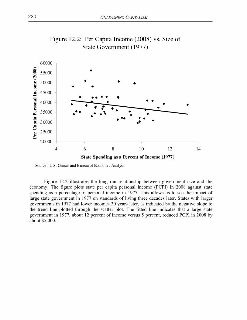
Figure 12.2 illustrates the long run relationship between government size and the economy. The figure plots state per capita personal income (PCPI) in 2008 against state spending as a percentage of personal income in 1977. This allows us to see the impact of large state government in 1977 on standards of living three decades later. States with larger governments in 1977 had lower incomes 30 years later, as indicated by the negative slope to the trend line plotted through the scatter plot. The fitted line indicates that a large state government in 1977, about 12 percent of income versus 5 percent, reduced PCPI in 2008 by about $5,000.
7
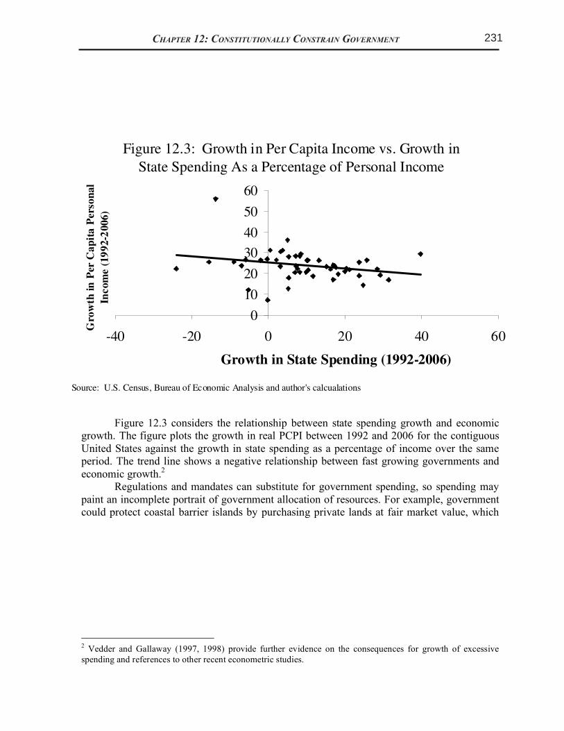
Figure 12.3 considers the relationship between state spending growth and economic
growth. The figure plots the growth in real PCPI between 1992 and 2006 for the contiguous United States against the growth in state spending as a percentage of income over the same period. The trend line shows a negative relationship between fast growing governments and economic growth.2 Regulations and mandates can substitute for government spending, so spending may paint an incomplete portrait of government allocation of resources. For example, government could protect coastal barrier islands by purchasing private lands at fair market value, which
2 Vedder and Gallaway (1997, 1998) provide further evidence on the consequences for growth of excessive
spending and references to other recent econometric studies.
7
Figure 12.3 considers the relationship between state spending growth and economic
growth. The figure plots the growth in real PCPI between 1992 and 2006 for the contiguous United States against the growth in state spending as a percentage of income over the same period. The trend line shows a negative relationship between fast growing governments and economic growth.2 Regulations and mandates can substitute for government spending, so spending may paint an incomplete portrait of government allocation of resources. For example, government could protect coastal barrier islands by purchasing private lands at fair market value, which
2 Vedder and Gallaway (1997, 1998) provide further evidence on the consequences for growth of excessive
spending and references to other recent econometric studies.
UNLEASHING CAPITALISM 18
manufacturing property tax in the country. In Figure 5.8 we present the effective property tax rates data for Southeastern states, for comparison. The ranks given for the states are out of all 50 states. The ‘net tax’ and ‘effective tax rate’ are calculated based on property valued at $25 million ($12.5 million in machinery and equipment, $12.5 million in inventories, and $2.5 million in fixtures). Notice that South Carolina’s effective tax rate on industrial property is over 7.8 times higher than the most industry-friendly state, Delaware. (Delaware is listed in the figure because it is the lowest-tax state.)
Figure 5.8: Industrial Property Taxes in Southeastern states*, 2007 State Rank (of 50) Net Tax Effective Tax Rate
South Carolina 1 $1,864,900 3.73%
Mississippi 4 $1,291,050 2.58%
Texas 6 $1,264,358 2.53%
Tennessee 10 $1,033,544 2.07%
West Virginia 14 $833,234 1.67%
Louisiana 17 $783,407 1.57%
Georgia 20 $760,381 1.52%
Florida 24 $677,683 1.36%
Alabama 35 $533,776 1.11%
North Carolina 37 $491,071 0.98%
Kentucky 47 $327,100 0.65%
Virginia 49 $241,498 0.48%
Delaware 50 $238,840 0.48%
Source: National Association of Manufacturers (2009) * Taxes measured in the states’ largest city only.
Importantly, South Carolina’s effective tax rate is almost 2.5 times greater than Georgia’s tax, and almost 4 times greater than North Carolina’s. This puts South Carolina at a serious disadvantage, in terms of its ability to attract and keep industry. Since South Carolina has the highest tax in the country on industrial property, it should be no surprise that it has one of the lowest per capita incomes and economic growth rates in the country. Although it is probably not critical that South Carolina set its tax rate to the lowest in the country, it should definitely make it at least competitive for the Southeast. Since Georgia’s rate is effectively 1.52 percent and North Carolina’s is just under 1 percent, a rate at around 1 percent might be sufficient to attract more industry. Working to reduce the various taxes applied to industry would seriously improve the state’s competitiveness. Such a significant reduction in taxes on industrial property would obviously lead to a reduction in tax revenues on industrial property, at least initially. However, the overall revenue may in fact increase once the growth rate in the state begins to pick up and more industry moves into the state. Furthermore, if the official tax rates are lowered, then the state
Figure 12.2: Per Capita Income (2008) vs. Size of
State Government (1977)
20000
25000
30000
35000
40000
45000
50000
55000
60000
4 6 8 10 12 14
State Spending as a Percent of Income (1977)
Per C
ap
tia
Pe
rso
na
l In
com
e (
20
08)
Source: U.S. Census and Bureau of Economic Analysis
7
Figure 12.3 considers the relationship between state spending growth and economic
growth. The figure plots the growth in real PCPI between 1992 and 2006 for the contiguous United States against the growth in state spending as a percentage of income over the same period. The trend line shows a negative relationship between fast growing governments and economic growth.2 Regulations and mandates can substitute for government spending, so spending may paint an incomplete portrait of government allocation of resources. For example, government could protect coastal barrier islands by purchasing private lands at fair market value, which
2 Vedder and Gallaway (1997, 1998) provide further evidence on the consequences for growth of excessive
spending and references to other recent econometric studies.
UNLEASHING CAPITALISM 18
manufacturing property tax in the country. In Figure 5.8 we present the effective property tax rates data for Southeastern states, for comparison. The ranks given for the states are out of all 50 states. The ‘net tax’ and ‘effective tax rate’ are calculated based on property valued at $25 million ($12.5 million in machinery and equipment, $12.5 million in inventories, and $2.5 million in fixtures). Notice that South Carolina’s effective tax rate on industrial property is over 7.8 times higher than the most industry-friendly state, Delaware. (Delaware is listed in the figure because it is the lowest-tax state.)
Figure 5.8: Industrial Property Taxes in Southeastern states*, 2007 State Rank (of 50) Net Tax Effective Tax Rate
South Carolina 1 $1,864,900 3.73%
Mississippi 4 $1,291,050 2.58%
Texas 6 $1,264,358 2.53%
Tennessee 10 $1,033,544 2.07%
West Virginia 14 $833,234 1.67%
Louisiana 17 $783,407 1.57%
Georgia 20 $760,381 1.52%
Florida 24 $677,683 1.36%
Alabama 35 $533,776 1.11%
North Carolina 37 $491,071 0.98%
Kentucky 47 $327,100 0.65%
Virginia 49 $241,498 0.48%
Delaware 50 $238,840 0.48%
Source: National Association of Manufacturers (2009) * Taxes measured in the states’ largest city only.
Importantly, South Carolina’s effective tax rate is almost 2.5 times greater than Georgia’s tax, and almost 4 times greater than North Carolina’s. This puts South Carolina at a serious disadvantage, in terms of its ability to attract and keep industry. Since South Carolina has the highest tax in the country on industrial property, it should be no surprise that it has one of the lowest per capita incomes and economic growth rates in the country. Although it is probably not critical that South Carolina set its tax rate to the lowest in the country, it should definitely make it at least competitive for the Southeast. Since Georgia’s rate is effectively 1.52 percent and North Carolina’s is just under 1 percent, a rate at around 1 percent might be sufficient to attract more industry. Working to reduce the various taxes applied to industry would seriously improve the state’s competitiveness. Such a significant reduction in taxes on industrial property would obviously lead to a reduction in tax revenues on industrial property, at least initially. However, the overall revenue may in fact increase once the growth rate in the state begins to pick up and more industry moves into the state. Furthermore, if the official tax rates are lowered, then the state
230 CHAPTER 5: SPECIFIC TAX REFORMS
13
Presumably the original intent of imposing a tax rate schedule with graduated marginal tax rates was to make the income tax progressive. However, what progressivity exists in the state’s income tax structure is due to the zero tax on the first $2,630 of income, and because of the graduated marginal tax rates. However, since the marginal tax rate increases over such small steps in income, as shown in Figure 5.5, most of the progressivity occurs at lower income levels, not higher levels of income. At higher income levels, the average tax rate hardly increases at all. This nature of the current tax is directly contradictory to the goal of progressivity. So although on the surface it appears that the tax satisfies the vertical equity condition, it really does this only at the lower income levels reducing the wealth of these lowest income taxpayers, not the intended consequence.
Figure 5.5: South Carolina income tax: Current tax rates compared to inflation-indexed rates, 2009
Current Income Tax
Rates/Brackets
Income Tax Rates/Brackets if 1959 Tax Schedule was Inflation Adjusted to
2009
Taxable Income Tax
Amount Average Tax Rate
Tax Amount
Average Tax Rate
$5,000 $71 1.42% $125 2.5%
$10,000 $290 2.90% $250 2.5%
$15,000 $604 4.03% $377 2.51%
$20,000 $954 4.77% $527 2.63%
$30,000 $1,654 5.51% $834 2.78%
$50,000 $3,054 6.10% $1,695 3.39%
$75,000 $4,804 6.41% $3,127 4.17%
$100,000 $6,554 6.56% $4,877 4.88%
$150,000 $10,054 6.70% $8,377 5.58%
$200,000 $13,554 6.77% $11,877 5.94%
Figure 5.5 also shows what the average tax rates are for various incomes and taxes
under the current tax system in South Carolina. In the right columns it also shows what the taxes and average tax rates would be if the 1959 tax tables were indexed for inflation. The figure clearly shows that the 1959 indexed tax rate structure is more uniformly progressive, especially at higher levels of incomes. It keeps tax rates extremely low for the lowest income individuals in the state. Figure 5.5 also shows that the current tax system charges all income groups more in taxes than an indexed rate schedule. The only exception is the $5,000 income earner in the table. As South Carolina income taxes continue to climb while the tax brackets remain stagnant, the state becomes a relatively high-tax state. This has a negative impact on
6
Figure 12.2: Per Capita Income (2008) vs. Size of
State Government (1977)
20,000
25,000
30,000
35,000
40,000
45,000
50,000
55,000
60,000
4 6 8 10 12 14
State Spending as a Percent of Income (1977)
Per
Cap
tia P
erso
nal In
com
e (2
008)
Source: U.S. Census and Bureau of Economic Analysis
Figure 12.2 illustrates the long run relationship between government size and the economy. The figure plots state per capita personal income (PCPI) in 2008 against state spending as a percentage of personal income in 1977. This allows us to see the impact of large state government in 1977 on standards of living three decades later. States with larger governments in 1977 had lower incomes 30 years later, as indicated by the negative slope to the trend line plotted through the scatter plot. The fitted line indicates that a large state government in 1977, about 12 percent of income versus 5 percent, reduced PCPI in 2008 by about $5,000.
7
Figure 12.3 considers the relationship between state spending growth and economic
growth. The figure plots the growth in real PCPI between 1992 and 2006 for the contiguous United States against the growth in state spending as a percentage of income over the same period. The trend line shows a negative relationship between fast growing governments and economic growth.2 Regulations and mandates can substitute for government spending, so spending may paint an incomplete portrait of government allocation of resources. For example, government could protect coastal barrier islands by purchasing private lands at fair market value, which
2 Vedder and Gallaway (1997, 1998) provide further evidence on the consequences for growth of excessive
spending and references to other recent econometric studies.
Chapter 12: Constitutionally Constrain government
Figure 12.3: Growth in Per Capita Income vs. Growth in
State Spending As a Percentage of Personal Income
0
10
20
30
40
50
60
-40 -20 0 20 40 60
Growth in State Spending (1992-2006)
Gro
wth
in
Per
Ca
pit
a P
ers
on
al
Incom
e (
19
92-2
006
)
Source: U.S. Census, Bureau of Economic Analysis and author's calcualations
7
Figure 12.3 considers the relationship between state spending growth and economic
growth. The figure plots the growth in real PCPI between 1992 and 2006 for the contiguous United States against the growth in state spending as a percentage of income over the same period. The trend line shows a negative relationship between fast growing governments and economic growth.2 Regulations and mandates can substitute for government spending, so spending may paint an incomplete portrait of government allocation of resources. For example, government could protect coastal barrier islands by purchasing private lands at fair market value, which
2 Vedder and Gallaway (1997, 1998) provide further evidence on the consequences for growth of excessive
spending and references to other recent econometric studies.
UNLEASHING CAPITALISM 18
manufacturing property tax in the country. In Figure 5.8 we present the effective property tax rates data for Southeastern states, for comparison. The ranks given for the states are out of all 50 states. The ‘net tax’ and ‘effective tax rate’ are calculated based on property valued at $25 million ($12.5 million in machinery and equipment, $12.5 million in inventories, and $2.5 million in fixtures). Notice that South Carolina’s effective tax rate on industrial property is over 7.8 times higher than the most industry-friendly state, Delaware. (Delaware is listed in the figure because it is the lowest-tax state.)
Figure 5.8: Industrial Property Taxes in Southeastern states*, 2007 State Rank (of 50) Net Tax Effective Tax Rate
South Carolina 1 $1,864,900 3.73%
Mississippi 4 $1,291,050 2.58%
Texas 6 $1,264,358 2.53%
Tennessee 10 $1,033,544 2.07%
West Virginia 14 $833,234 1.67%
Louisiana 17 $783,407 1.57%
Georgia 20 $760,381 1.52%
Florida 24 $677,683 1.36%
Alabama 35 $533,776 1.11%
North Carolina 37 $491,071 0.98%
Kentucky 47 $327,100 0.65%
Virginia 49 $241,498 0.48%
Delaware 50 $238,840 0.48%
Source: National Association of Manufacturers (2009) * Taxes measured in the states’ largest city only.
Importantly, South Carolina’s effective tax rate is almost 2.5 times greater than Georgia’s tax, and almost 4 times greater than North Carolina’s. This puts South Carolina at a serious disadvantage, in terms of its ability to attract and keep industry. Since South Carolina has the highest tax in the country on industrial property, it should be no surprise that it has one of the lowest per capita incomes and economic growth rates in the country. Although it is probably not critical that South Carolina set its tax rate to the lowest in the country, it should definitely make it at least competitive for the Southeast. Since Georgia’s rate is effectively 1.52 percent and North Carolina’s is just under 1 percent, a rate at around 1 percent might be sufficient to attract more industry. Working to reduce the various taxes applied to industry would seriously improve the state’s competitiveness. Such a significant reduction in taxes on industrial property would obviously lead to a reduction in tax revenues on industrial property, at least initially. However, the overall revenue may in fact increase once the growth rate in the state begins to pick up and more industry moves into the state. Furthermore, if the official tax rates are lowered, then the state
231CHAPTER 5: SPECIFIC TAX REFORMS
13
Presumably the original intent of imposing a tax rate schedule with graduated marginal tax rates was to make the income tax progressive. However, what progressivity exists in the state’s income tax structure is due to the zero tax on the first $2,630 of income, and because of the graduated marginal tax rates. However, since the marginal tax rate increases over such small steps in income, as shown in Figure 5.5, most of the progressivity occurs at lower income levels, not higher levels of income. At higher income levels, the average tax rate hardly increases at all. This nature of the current tax is directly contradictory to the goal of progressivity. So although on the surface it appears that the tax satisfies the vertical equity condition, it really does this only at the lower income levels reducing the wealth of these lowest income taxpayers, not the intended consequence.
Figure 5.5: South Carolina income tax: Current tax rates compared to inflation-indexed rates, 2009
Current Income Tax
Rates/Brackets
Income Tax Rates/Brackets if 1959 Tax Schedule was Inflation Adjusted to
2009
Taxable Income Tax
Amount Average Tax Rate
Tax Amount
Average Tax Rate
$5,000 $71 1.42% $125 2.5%
$10,000 $290 2.90% $250 2.5%
$15,000 $604 4.03% $377 2.51%
$20,000 $954 4.77% $527 2.63%
$30,000 $1,654 5.51% $834 2.78%
$50,000 $3,054 6.10% $1,695 3.39%
$75,000 $4,804 6.41% $3,127 4.17%
$100,000 $6,554 6.56% $4,877 4.88%
$150,000 $10,054 6.70% $8,377 5.58%
$200,000 $13,554 6.77% $11,877 5.94%
Figure 5.5 also shows what the average tax rates are for various incomes and taxes
under the current tax system in South Carolina. In the right columns it also shows what the taxes and average tax rates would be if the 1959 tax tables were indexed for inflation. The figure clearly shows that the 1959 indexed tax rate structure is more uniformly progressive, especially at higher levels of incomes. It keeps tax rates extremely low for the lowest income individuals in the state. Figure 5.5 also shows that the current tax system charges all income groups more in taxes than an indexed rate schedule. The only exception is the $5,000 income earner in the table. As South Carolina income taxes continue to climb while the tax brackets remain stagnant, the state becomes a relatively high-tax state. This has a negative impact on
8
would involve a substantial expenditure, or simply prohibit owners from developing their property. Regulation affects the use of private property as surely as if the state government had purchased the lands. Thus the evidence on state economic freedom and growth discussed in Chapter 2 is relevant to our topic. Lower economic freedom, even at the subnational level, reduces income and slows growth.
Figure 12.4: Economic Freedom: South Carolina and Its Neighbors
State Overall Index Size of Government
Takings and Discriminatory Taxation
Labor Market
South Carolina 6.8 (T-25th) 6.0 (T-40th) 6.7 (T-34th) 8.4 (T-1st)
North Carolina 7.6 (T-3rd) 7.5 (T-14th) 7.5 (T-11th) 7.3 (9th)
Georgia 7.6 (T-3rd) 7.7 (12th) 7.5 (T-11th) 7.4 (T-10th)
U.S. Average 6.9 6.9 7.0 6.8 Source: Karabegovic and McMahon (2008).
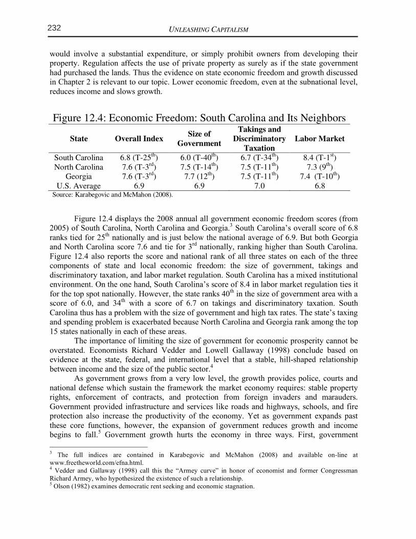
Figure 12.4 displays the 2008 annual all government economic freedom scores (from
2005) of South Carolina, North Carolina and Georgia.3 South Carolina’s overall score of 6.8 ranks tied for 25th nationally and is just below the national average of 6.9. But both Georgia and North Carolina score 7.6 and tie for 3rd nationally, ranking higher than South Carolina. Figure 12.4 also reports the score and national rank of all three states on each of the three components of state and local economic freedom: the size of government, takings and discriminatory taxation, and labor market regulation. South Carolina has a mixed institutional environment. On the one hand, South Carolina’s score of 8.4 in labor market regulation ties it for the top spot nationally. However, the state ranks 40th in the size of government area with a score of 6.0, and 34th with a score of 6.7 on takings and discriminatory taxation. South Carolina thus has a problem with the size of government and high tax rates. The state’s taxing and spending problem is exacerbated because North Carolina and Georgia rank among the top 15 states nationally in each of these areas. The importance of limiting the size of government for economic prosperity cannot be overstated. Economists Richard Vedder and Lowell Gallaway (1998) conclude based on evidence at the state, federal, and international level that a stable, hill-shaped relationship between income and the size of the public sector.4
As government grows from a very low level, the growth provides police, courts and national defense which sustain the framework the market economy requires: stable property rights, enforcement of contracts, and protection from foreign invaders and marauders. Government provided infrastructure and services like roads and highways, schools, and fire protection also increase the productivity of the economy. Yet as government expands past these core functions, however, the expansion of government reduces growth and income begins to fall.5 Government growth hurts the economy in three ways. First, government
3 The full indices are contained in Karabegovic and McMahon (2008) and available on-line at
www.freetheworld.com/efna.html. 4 Vedder and Gallaway (1998) call this the “Armey curve” in honor of economist and former Congressman
Richard Armey, who hypothesized the existence of such a relationship. 5 Olson (1982) examines democratic rent seeking and economic stagnation.
9
increasingly makes resource allocation decisions, and these decisions are made for political reasons, not profit or loss considerations. Second, government must tax to fund spending. Taxes distort choices in the market, and the cost to the economy of this distortion exceeds the dollars collected for government to spend. Higher taxes reduce economic freedom, entrepreneurship (Garrett and Wall 2006), and growth (Poulson and Kaplan 2008). Marginal tax rates, the tax people pay if they earn an extra $1,000 or if a business earns an extra $1 million in profit, determine how much taxes reduce economic activity. The disruptive effect of taxes increases more than proportionally with the tax rate, so that the distortion from a 20 percent income tax rate is more than double that from a 10 percent. Vedder and Gallaway (1999) contend based on the available evidence that the cost of taxes may be 40 cents or more per dollar of revenue raised. Third, interest groups use resources to lobby politicians for increased spending, what Gordon Tullock (1967) labeled ‘rent seeking.’ Resources spent trying to secure favors from government cannot be used to produce things of value like cars, clothes, homes, and computers, making society poorer.
ENTREPRENEURSHIP: TURNING ECONOMIC FREEDOM INTO
PROSPERITY
Economists have made considerable progress over the past several years establishing entrepreneurship as the link between economic freedom and prosperity. This is not surprising as previously economists like Joseph Schumpeter, Ludwig von Mises, and Israel Kirzner argued that the entrepreneur is the agent of creative destruction and progress in the market economy. The entrepreneur is the source of ideas for new or improved products, new uses for existing products, and new forms of economic organization. Entrepreneurship requires a free market, because we cannot know what new ideas will be discovered, or from where these ideas will come. Recent research documents how economic freedom increases entrepreneurship, using a variety of different measures of entrepreneurial activity, including the number of sole proprietorships, net business formation, patents, and venture capital.6 Taxes and regulations like minimum wages particularly (which affect economic freedom) negatively impact entrepreneurship.
Figure 12.5: Economic Freedom and Entrepreneurship
Measure of Entrepreneurship
State Ranked on Economic Freedom
Index of Productive Entrepreneurship
Percentage of Sole Proprietorships, 1990 & 2000
Most Free 29.2 15.0
Least Free 21.4 14.8 Sources: Karabegovic and McMahon (2008), Sobel (2008), Garrett and Wall (2006).
6 For evidence on the relationship between economic freedom and entrepreneurship see Kreft and Sobel (2005),
Garrett and Wall (2006), Campbell and Rodgers (2007), and Sobel (2008).
UNLEASHING CAPITALISM 18
manufacturing property tax in the country. In Figure 5.8 we present the effective property tax rates data for Southeastern states, for comparison. The ranks given for the states are out of all 50 states. The ‘net tax’ and ‘effective tax rate’ are calculated based on property valued at $25 million ($12.5 million in machinery and equipment, $12.5 million in inventories, and $2.5 million in fixtures). Notice that South Carolina’s effective tax rate on industrial property is over 7.8 times higher than the most industry-friendly state, Delaware. (Delaware is listed in the figure because it is the lowest-tax state.)
Figure 5.8: Industrial Property Taxes in Southeastern states*, 2007 State Rank (of 50) Net Tax Effective Tax Rate
South Carolina 1 $1,864,900 3.73%
Mississippi 4 $1,291,050 2.58%
Texas 6 $1,264,358 2.53%
Tennessee 10 $1,033,544 2.07%
West Virginia 14 $833,234 1.67%
Louisiana 17 $783,407 1.57%
Georgia 20 $760,381 1.52%
Florida 24 $677,683 1.36%
Alabama 35 $533,776 1.11%
North Carolina 37 $491,071 0.98%
Kentucky 47 $327,100 0.65%
Virginia 49 $241,498 0.48%
Delaware 50 $238,840 0.48%
Source: National Association of Manufacturers (2009) * Taxes measured in the states’ largest city only.
Importantly, South Carolina’s effective tax rate is almost 2.5 times greater than Georgia’s tax, and almost 4 times greater than North Carolina’s. This puts South Carolina at a serious disadvantage, in terms of its ability to attract and keep industry. Since South Carolina has the highest tax in the country on industrial property, it should be no surprise that it has one of the lowest per capita incomes and economic growth rates in the country. Although it is probably not critical that South Carolina set its tax rate to the lowest in the country, it should definitely make it at least competitive for the Southeast. Since Georgia’s rate is effectively 1.52 percent and North Carolina’s is just under 1 percent, a rate at around 1 percent might be sufficient to attract more industry. Working to reduce the various taxes applied to industry would seriously improve the state’s competitiveness. Such a significant reduction in taxes on industrial property would obviously lead to a reduction in tax revenues on industrial property, at least initially. However, the overall revenue may in fact increase once the growth rate in the state begins to pick up and more industry moves into the state. Furthermore, if the official tax rates are lowered, then the state
Figure 12.4: Economic Freedom: South Carolina and Its Neighbors
State Overall Index Size of
Government
Takings and
Discriminatory
Taxation
Labor Market
South Carolina 6.8 (T-25th) 6.0 (T-40
th) 6.7 (T-34
th) 8.4 (T-1
st)
North Carolina 7.6 (T-3rd
) 7.5 (T-14th) 7.5 (T-11
th) 7.3 (9
th)
Georgia 7.6 (T-3rd
) 7.7 (12th) 7.5 (T-11
th) 7.4 (T-10
th)
U.S. Average 6.9 6.9 7.0 6.8 Source: Karabegovic and McMahon (2008).
Figure 12.5: Economic Freedom and Entrepreneurship Measure of Entrepreneurship
State Ranked on
Economic Freedom
Index of Productive
Entrepreneurship
Percentage of Sole
Proprietorships, 1990 &
2000
Most Free 29.2 15.0
Least Free 21.4 14.8 Sources: Karabegovic and McMahon (2008), Sobel (2008), Garrett and Wall (2006).
UNLEASHING CAPITALISM 18
manufacturing property tax in the country. In Figure 5.8 we present the effective property tax rates data for Southeastern states, for comparison. The ranks given for the states are out of all 50 states. The ‘net tax’ and ‘effective tax rate’ are calculated based on property valued at $25 million ($12.5 million in machinery and equipment, $12.5 million in inventories, and $2.5 million in fixtures). Notice that South Carolina’s effective tax rate on industrial property is over 7.8 times higher than the most industry-friendly state, Delaware. (Delaware is listed in the figure because it is the lowest-tax state.)
Figure 5.8: Industrial Property Taxes in Southeastern states*, 2007 State Rank (of 50) Net Tax Effective Tax Rate
South Carolina 1 $1,864,900 3.73%
Mississippi 4 $1,291,050 2.58%
Texas 6 $1,264,358 2.53%
Tennessee 10 $1,033,544 2.07%
West Virginia 14 $833,234 1.67%
Louisiana 17 $783,407 1.57%
Georgia 20 $760,381 1.52%
Florida 24 $677,683 1.36%
Alabama 35 $533,776 1.11%
North Carolina 37 $491,071 0.98%
Kentucky 47 $327,100 0.65%
Virginia 49 $241,498 0.48%
Delaware 50 $238,840 0.48%
Source: National Association of Manufacturers (2009) * Taxes measured in the states’ largest city only.
Importantly, South Carolina’s effective tax rate is almost 2.5 times greater than Georgia’s tax, and almost 4 times greater than North Carolina’s. This puts South Carolina at a serious disadvantage, in terms of its ability to attract and keep industry. Since South Carolina has the highest tax in the country on industrial property, it should be no surprise that it has one of the lowest per capita incomes and economic growth rates in the country. Although it is probably not critical that South Carolina set its tax rate to the lowest in the country, it should definitely make it at least competitive for the Southeast. Since Georgia’s rate is effectively 1.52 percent and North Carolina’s is just under 1 percent, a rate at around 1 percent might be sufficient to attract more industry. Working to reduce the various taxes applied to industry would seriously improve the state’s competitiveness. Such a significant reduction in taxes on industrial property would obviously lead to a reduction in tax revenues on industrial property, at least initially. However, the overall revenue may in fact increase once the growth rate in the state begins to pick up and more industry moves into the state. Furthermore, if the official tax rates are lowered, then the state
232 CHAPTER 5: SPECIFIC TAX REFORMS
13
Presumably the original intent of imposing a tax rate schedule with graduated marginal tax rates was to make the income tax progressive. However, what progressivity exists in the state’s income tax structure is due to the zero tax on the first $2,630 of income, and because of the graduated marginal tax rates. However, since the marginal tax rate increases over such small steps in income, as shown in Figure 5.5, most of the progressivity occurs at lower income levels, not higher levels of income. At higher income levels, the average tax rate hardly increases at all. This nature of the current tax is directly contradictory to the goal of progressivity. So although on the surface it appears that the tax satisfies the vertical equity condition, it really does this only at the lower income levels reducing the wealth of these lowest income taxpayers, not the intended consequence.
Figure 5.5: South Carolina income tax: Current tax rates compared to inflation-indexed rates, 2009
Current Income Tax
Rates/Brackets
Income Tax Rates/Brackets if 1959 Tax Schedule was Inflation Adjusted to
2009
Taxable Income Tax
Amount Average Tax Rate
Tax Amount
Average Tax Rate
$5,000 $71 1.42% $125 2.5%
$10,000 $290 2.90% $250 2.5%
$15,000 $604 4.03% $377 2.51%
$20,000 $954 4.77% $527 2.63%
$30,000 $1,654 5.51% $834 2.78%
$50,000 $3,054 6.10% $1,695 3.39%
$75,000 $4,804 6.41% $3,127 4.17%
$100,000 $6,554 6.56% $4,877 4.88%
$150,000 $10,054 6.70% $8,377 5.58%
$200,000 $13,554 6.77% $11,877 5.94%
Figure 5.5 also shows what the average tax rates are for various incomes and taxes
under the current tax system in South Carolina. In the right columns it also shows what the taxes and average tax rates would be if the 1959 tax tables were indexed for inflation. The figure clearly shows that the 1959 indexed tax rate structure is more uniformly progressive, especially at higher levels of incomes. It keeps tax rates extremely low for the lowest income individuals in the state. Figure 5.5 also shows that the current tax system charges all income groups more in taxes than an indexed rate schedule. The only exception is the $5,000 income earner in the table. As South Carolina income taxes continue to climb while the tax brackets remain stagnant, the state becomes a relatively high-tax state. This has a negative impact on
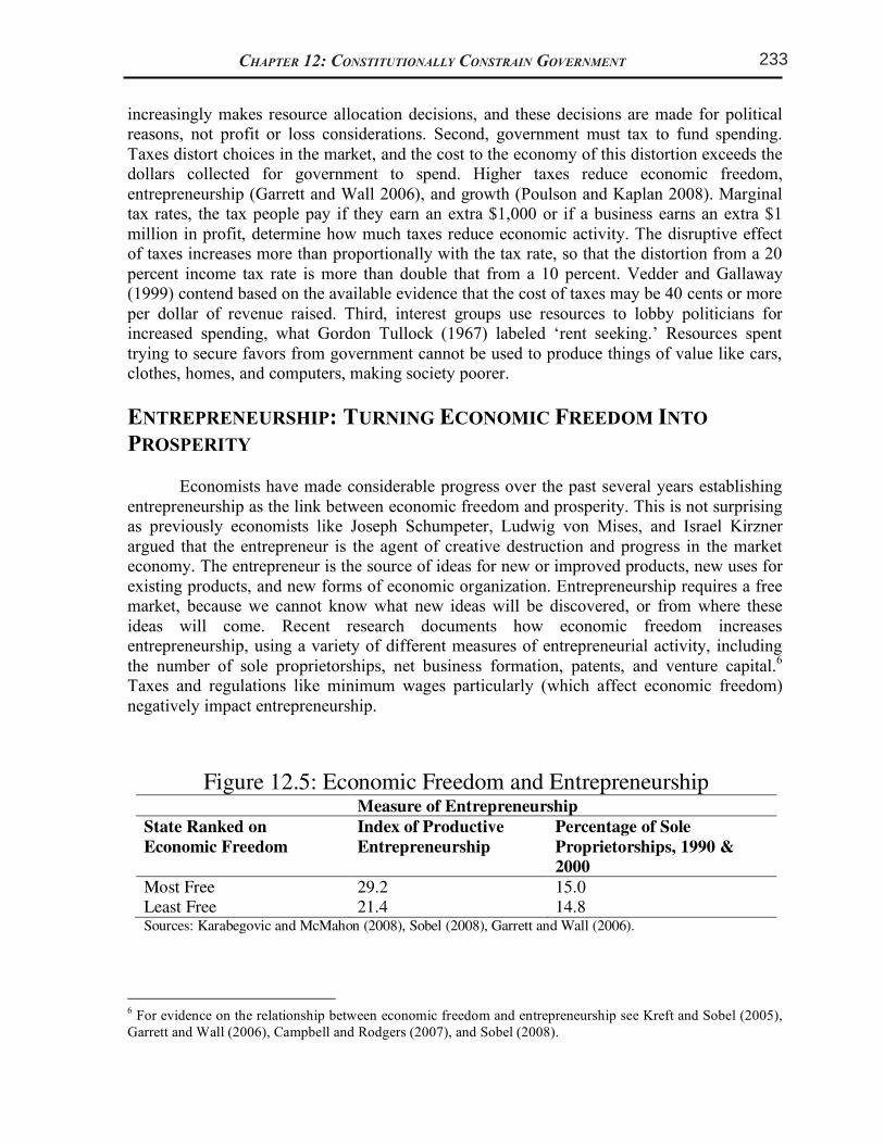
8
would involve a substantial expenditure, or simply prohibit owners from developing their property. Regulation affects the use of private property as surely as if the state government had purchased the lands. Thus the evidence on state economic freedom and growth discussed in Chapter 2 is relevant to our topic. Lower economic freedom, even at the subnational level, reduces income and slows growth.
Figure 12.4: Economic Freedom: South Carolina and Its Neighbors
State Overall Index Size of Government
Takings and Discriminatory Taxation
Labor Market
South Carolina 6.8 (T-25th) 6.0 (T-40th) 6.7 (T-34th) 8.4 (T-1st)
North Carolina 7.6 (T-3rd) 7.5 (T-14th) 7.5 (T-11th) 7.3 (9th)
Georgia 7.6 (T-3rd) 7.7 (12th) 7.5 (T-11th) 7.4 (T-10th)
U.S. Average 6.9 6.9 7.0 6.8 Source: Karabegovic and McMahon (2008).
Figure 12.4 displays the 2008 annual all government economic freedom scores (from
2005) of South Carolina, North Carolina and Georgia.3 South Carolina’s overall score of 6.8 ranks tied for 25th nationally and is just below the national average of 6.9. But both Georgia and North Carolina score 7.6 and tie for 3rd nationally, ranking higher than South Carolina. Figure 12.4 also reports the score and national rank of all three states on each of the three components of state and local economic freedom: the size of government, takings and discriminatory taxation, and labor market regulation. South Carolina has a mixed institutional environment. On the one hand, South Carolina’s score of 8.4 in labor market regulation ties it for the top spot nationally. However, the state ranks 40th in the size of government area with a score of 6.0, and 34th with a score of 6.7 on takings and discriminatory taxation. South Carolina thus has a problem with the size of government and high tax rates. The state’s taxing and spending problem is exacerbated because North Carolina and Georgia rank among the top 15 states nationally in each of these areas. The importance of limiting the size of government for economic prosperity cannot be overstated. Economists Richard Vedder and Lowell Gallaway (1998) conclude based on evidence at the state, federal, and international level that a stable, hill-shaped relationship between income and the size of the public sector.4
As government grows from a very low level, the growth provides police, courts and national defense which sustain the framework the market economy requires: stable property rights, enforcement of contracts, and protection from foreign invaders and marauders. Government provided infrastructure and services like roads and highways, schools, and fire protection also increase the productivity of the economy. Yet as government expands past these core functions, however, the expansion of government reduces growth and income begins to fall.5 Government growth hurts the economy in three ways. First, government
3 The full indices are contained in Karabegovic and McMahon (2008) and available on-line at
www.freetheworld.com/efna.html. 4 Vedder and Gallaway (1998) call this the “Armey curve” in honor of economist and former Congressman
Richard Armey, who hypothesized the existence of such a relationship. 5 Olson (1982) examines democratic rent seeking and economic stagnation.
9
increasingly makes resource allocation decisions, and these decisions are made for political reasons, not profit or loss considerations. Second, government must tax to fund spending. Taxes distort choices in the market, and the cost to the economy of this distortion exceeds the dollars collected for government to spend. Higher taxes reduce economic freedom, entrepreneurship (Garrett and Wall 2006), and growth (Poulson and Kaplan 2008). Marginal tax rates, the tax people pay if they earn an extra $1,000 or if a business earns an extra $1 million in profit, determine how much taxes reduce economic activity. The disruptive effect of taxes increases more than proportionally with the tax rate, so that the distortion from a 20 percent income tax rate is more than double that from a 10 percent. Vedder and Gallaway (1999) contend based on the available evidence that the cost of taxes may be 40 cents or more per dollar of revenue raised. Third, interest groups use resources to lobby politicians for increased spending, what Gordon Tullock (1967) labeled ‘rent seeking.’ Resources spent trying to secure favors from government cannot be used to produce things of value like cars, clothes, homes, and computers, making society poorer.
ENTREPRENEURSHIP: TURNING ECONOMIC FREEDOM INTO
PROSPERITY
Economists have made considerable progress over the past several years establishing entrepreneurship as the link between economic freedom and prosperity. This is not surprising as previously economists like Joseph Schumpeter, Ludwig von Mises, and Israel Kirzner argued that the entrepreneur is the agent of creative destruction and progress in the market economy. The entrepreneur is the source of ideas for new or improved products, new uses for existing products, and new forms of economic organization. Entrepreneurship requires a free market, because we cannot know what new ideas will be discovered, or from where these ideas will come. Recent research documents how economic freedom increases entrepreneurship, using a variety of different measures of entrepreneurial activity, including the number of sole proprietorships, net business formation, patents, and venture capital.6 Taxes and regulations like minimum wages particularly (which affect economic freedom) negatively impact entrepreneurship.
Figure 12.5: Economic Freedom and Entrepreneurship
Measure of Entrepreneurship
State Ranked on Economic Freedom
Index of Productive Entrepreneurship
Percentage of Sole Proprietorships, 1990 & 2000
Most Free 29.2 15.0
Least Free 21.4 14.8 Sources: Karabegovic and McMahon (2008), Sobel (2008), Garrett and Wall (2006).
6 For evidence on the relationship between economic freedom and entrepreneurship see Kreft and Sobel (2005),
Garrett and Wall (2006), Campbell and Rodgers (2007), and Sobel (2008).
Chapter 12: Constitutionally Constrain government
Figure 12.4: Economic Freedom: South Carolina and Its Neighbors
State Overall Index Size of
Government
Takings and
Discriminatory
Taxation
Labor Market
South Carolina 6.8 (T-25th) 6.0 (T-40
th) 6.7 (T-34
th) 8.4 (T-1
st)
North Carolina 7.6 (T-3rd
) 7.5 (T-14th) 7.5 (T-11
th) 7.3 (9
th)
Georgia 7.6 (T-3rd
) 7.7 (12th) 7.5 (T-11
th) 7.4 (T-10
th)
U.S. Average 6.9 6.9 7.0 6.8 Source: Karabegovic and McMahon (2008).
Figure 12.5: Economic Freedom and Entrepreneurship Measure of Entrepreneurship
State Ranked on
Economic Freedom
Index of Productive
Entrepreneurship
Percentage of Sole
Proprietorships, 1990 &
2000
Most Free 29.2 15.0
Least Free 21.4 14.8 Sources: Karabegovic and McMahon (2008), Sobel (2008), Garrett and Wall (2006).
UNLEASHING CAPITALISM 18
manufacturing property tax in the country. In Figure 5.8 we present the effective property tax rates data for Southeastern states, for comparison. The ranks given for the states are out of all 50 states. The ‘net tax’ and ‘effective tax rate’ are calculated based on property valued at $25 million ($12.5 million in machinery and equipment, $12.5 million in inventories, and $2.5 million in fixtures). Notice that South Carolina’s effective tax rate on industrial property is over 7.8 times higher than the most industry-friendly state, Delaware. (Delaware is listed in the figure because it is the lowest-tax state.)
Figure 5.8: Industrial Property Taxes in Southeastern states*, 2007 State Rank (of 50) Net Tax Effective Tax Rate
South Carolina 1 $1,864,900 3.73%
Mississippi 4 $1,291,050 2.58%
Texas 6 $1,264,358 2.53%
Tennessee 10 $1,033,544 2.07%
West Virginia 14 $833,234 1.67%
Louisiana 17 $783,407 1.57%
Georgia 20 $760,381 1.52%
Florida 24 $677,683 1.36%
Alabama 35 $533,776 1.11%
North Carolina 37 $491,071 0.98%
Kentucky 47 $327,100 0.65%
Virginia 49 $241,498 0.48%
Delaware 50 $238,840 0.48%
Source: National Association of Manufacturers (2009) * Taxes measured in the states’ largest city only.
Importantly, South Carolina’s effective tax rate is almost 2.5 times greater than Georgia’s tax, and almost 4 times greater than North Carolina’s. This puts South Carolina at a serious disadvantage, in terms of its ability to attract and keep industry. Since South Carolina has the highest tax in the country on industrial property, it should be no surprise that it has one of the lowest per capita incomes and economic growth rates in the country. Although it is probably not critical that South Carolina set its tax rate to the lowest in the country, it should definitely make it at least competitive for the Southeast. Since Georgia’s rate is effectively 1.52 percent and North Carolina’s is just under 1 percent, a rate at around 1 percent might be sufficient to attract more industry. Working to reduce the various taxes applied to industry would seriously improve the state’s competitiveness. Such a significant reduction in taxes on industrial property would obviously lead to a reduction in tax revenues on industrial property, at least initially. However, the overall revenue may in fact increase once the growth rate in the state begins to pick up and more industry moves into the state. Furthermore, if the official tax rates are lowered, then the state
233CHAPTER 5: SPECIFIC TAX REFORMS
13
Presumably the original intent of imposing a tax rate schedule with graduated marginal tax rates was to make the income tax progressive. However, what progressivity exists in the state’s income tax structure is due to the zero tax on the first $2,630 of income, and because of the graduated marginal tax rates. However, since the marginal tax rate increases over such small steps in income, as shown in Figure 5.5, most of the progressivity occurs at lower income levels, not higher levels of income. At higher income levels, the average tax rate hardly increases at all. This nature of the current tax is directly contradictory to the goal of progressivity. So although on the surface it appears that the tax satisfies the vertical equity condition, it really does this only at the lower income levels reducing the wealth of these lowest income taxpayers, not the intended consequence.
Figure 5.5: South Carolina income tax: Current tax rates compared to inflation-indexed rates, 2009
Current Income Tax
Rates/Brackets
Income Tax Rates/Brackets if 1959 Tax Schedule was Inflation Adjusted to
2009
Taxable Income Tax
Amount Average Tax Rate
Tax Amount
Average Tax Rate
$5,000 $71 1.42% $125 2.5%
$10,000 $290 2.90% $250 2.5%
$15,000 $604 4.03% $377 2.51%
$20,000 $954 4.77% $527 2.63%
$30,000 $1,654 5.51% $834 2.78%
$50,000 $3,054 6.10% $1,695 3.39%
$75,000 $4,804 6.41% $3,127 4.17%
$100,000 $6,554 6.56% $4,877 4.88%
$150,000 $10,054 6.70% $8,377 5.58%
$200,000 $13,554 6.77% $11,877 5.94%
Figure 5.5 also shows what the average tax rates are for various incomes and taxes
under the current tax system in South Carolina. In the right columns it also shows what the taxes and average tax rates would be if the 1959 tax tables were indexed for inflation. The figure clearly shows that the 1959 indexed tax rate structure is more uniformly progressive, especially at higher levels of incomes. It keeps tax rates extremely low for the lowest income individuals in the state. Figure 5.5 also shows that the current tax system charges all income groups more in taxes than an indexed rate schedule. The only exception is the $5,000 income earner in the table. As South Carolina income taxes continue to climb while the tax brackets remain stagnant, the state becomes a relatively high-tax state. This has a negative impact on
10
Figure 12.5 illustrates the impact of economic freedom on two measures of entrepreneurship, sole proprietorships as reported by Garrett and Wall (2006), and an index of productive entrepreneurship constructed by Sobel (2008). The Figure compares the mean levels of entrepreneurship in the five states with the highest economic freedom scores and five states with the lowest economic freedom scores (plus ties in each case). South Carolina faces an entrepreneurship deficit. The state ranked tied for last with Mississippi in sole proprietorships in 1990 and ahead of only West Virginia in 2000 (Garrett and Wall 2008), and tied for 29th in Sobel’s (2008) index of productive entrepreneurship. The entrepreneurship deficit must be closed for South Carolina to capture the full benefits of the market economy. Can South Carolina take direct steps to generate entrepreneurship? Would-be entrepreneurs will point out that they could start new businesses if they could obtain access to venture capital or other types of subsidies. State development policies were examined in detail in Chapter 7, and have an indistinguished record. Development incentives often disadvantage new and small businesses, which lack the political clout to obtain such favors, and face higher taxes to pay for the programs. Kreft and Sobel (2005) specifically examine the relationship between venture capital and entrepreneurship across states and found that entrepreneurship attracts venture capital, while an increase in venture capital does not increase entrepreneurship. Kreft and Sobel (2005, 603) observe, “entrepreneurial activity must be the focus of development efforts and venture funding will automatically, and naturally flow into the area to support this activity.” Entrepreneurship requires ideas and alertness for new profit opportunities, tasks for which state governments have no comparative advantage. Politicization of the economy affects entrepreneurship in a second way beyond simply disrupting productive, wealth-generating activities. The human drive for self-improvement does not disappear as opportunities to pursue profit in the market are blocked. Instead, as William Baumol (1990) has argued, and as examined in Chapter 2, politicization of the economy shifts entrepreneurship to socially unproductive forms like litigation or the pursuit of government subsidies and favors. The same creativity, alertness and intelligence which generate new wealth for the economy under good institutions become a drain on the productive economy. We see political entrepreneurship at work when companies exploit state development incentives, and in the successful efforts of banks and automakers to obtain government bailouts.
THE IMPERFECTIONS OF POLITICS AND EXCESSIVE GOVERNMENT
SPENDING
The economic analysis of institutions and growth demonstrates what government must do to facilitate growth: maintain secure property rights, provide an efficient court system, and supply important public goods like national defense or infrastructure. Then government must avoid politicizing the economy, by taxing, spending, and regulating too much. South Carolina particularly must control government spending and addressing its entrepreneurship deficit. It might seem that in order to unleash capitalism, South Carolina voters need to work to elect politicians who will reduce spending. Yet direct political action, paradoxically, is unlikely to attain this goal. To understand why, we must consider insights from the application of economic analysis to the political
11
process, or public choice economics. The vision of democracy emerging from public choice scholarship contrasts sharply with the high school civics class. Political decision making suffers from a number of serious problems in comparison with market decision making and these problems lead government to spend too much, that is, more than the average citizen would like government to spend. Representative government results in a budget which is not merely larger than fiscal conservatives’ desire, but larger than the majority of voters prefer. Democratic politics fails to deliver a government of the size we desire.7 The first element of politics leading to excessive spending is the considerable power to shape government decisions possessed by political agenda setters. Politics is like sports in that match ups matter. Some teams match up very well against some opponents but very poorly against others. If you could set the matchups in a playoff tournament, you could create a bracket to help your favorite team. You could go a long way toward getting your favorite team to the championship merely by setting the matchups, even without blatantly cheating in your team’s favor (e.g., making their opponents play short handed). A similar dynamic prevails in politics. Legislators can limit what bills their colleagues get to vote on, or if their colleagues can offer amendments during floor debate. Legislative leaders can assign a bill they oppose to a hostile committee to ensure that the bill dies; agenda setting explains why the majority party in Congress or a state legislature has so much power. Politicians and bureaucrats can also manipulate the ballot propositions and tax measures which citizens get to vote on in elections. Voting and elections never pin down one outcome, allowing politicians to influence the eventual outcome. Given that politicians can benefit from spending money (providing benefits to grateful constituents or bureaucrats), they will take advantage of agenda power to increase government spending. We live in a representative and not a direct democracy, and this creates a second problem, the control of politicians. A legislator can pursue his or her interests at constituents’ expense on some issues because voters have only relatively weak means to control politicians. Reelection is the main incentive citizens have to control their representatives; other types of political action like sending letters or making phone calls and working for (or contributing to) a candidate eventually affect reelection prospects. Yet we elect legislators once every two or four years. Consequently all the votes, committee work, bills sponsored and hearings held over two (or four) years by an incumbent legislator must be combined into one vote for or against, and turning out the incumbent may mean electing a weak opponent. Citizens might have one or two issues which matter most to them, and vote for or against their legislator based on their position on these issues. Beyond one’s vote, the citizen has no further leverage to reward or punish any other actions by their representative. By contrast, firms can have their employees work for a salary, or on commission, or pay bonuses based on profit or team performance, offer promotions and raises, and terminate employment relatively quickly for unacceptable performance. One election every two years is a poor control, leaving legislators comparatively broad discretion to pursue policies that either they or special interest groups prefer at the expense of constituents. The third problem of politics is a lack of decisiveness for individual action, that is, individuals can not directly decide political outcomes. In the market, our choices or actions decide what happens to us, largely if not totally. For example, if you choose to buy soft drinks
7 The classic public choice analysis of democracy is Buchanan and Tullock (1962). Mueller (2003) provides a
recent synthesis and overview, while Mitchell and Simmons (1994) provide a very readable treatment. For an
analysis of the differences in the pathologies of politics at the level of the individual citizen, see Caplan (2007).
UNLEASHING CAPITALISM 18
manufacturing property tax in the country. In Figure 5.8 we present the effective property tax rates data for Southeastern states, for comparison. The ranks given for the states are out of all 50 states. The ‘net tax’ and ‘effective tax rate’ are calculated based on property valued at $25 million ($12.5 million in machinery and equipment, $12.5 million in inventories, and $2.5 million in fixtures). Notice that South Carolina’s effective tax rate on industrial property is over 7.8 times higher than the most industry-friendly state, Delaware. (Delaware is listed in the figure because it is the lowest-tax state.)
Figure 5.8: Industrial Property Taxes in Southeastern states*, 2007 State Rank (of 50) Net Tax Effective Tax Rate
South Carolina 1 $1,864,900 3.73%
Mississippi 4 $1,291,050 2.58%
Texas 6 $1,264,358 2.53%
Tennessee 10 $1,033,544 2.07%
West Virginia 14 $833,234 1.67%
Louisiana 17 $783,407 1.57%
Georgia 20 $760,381 1.52%
Florida 24 $677,683 1.36%
Alabama 35 $533,776 1.11%
North Carolina 37 $491,071 0.98%
Kentucky 47 $327,100 0.65%
Virginia 49 $241,498 0.48%
Delaware 50 $238,840 0.48%
Source: National Association of Manufacturers (2009) * Taxes measured in the states’ largest city only.
Importantly, South Carolina’s effective tax rate is almost 2.5 times greater than Georgia’s tax, and almost 4 times greater than North Carolina’s. This puts South Carolina at a serious disadvantage, in terms of its ability to attract and keep industry. Since South Carolina has the highest tax in the country on industrial property, it should be no surprise that it has one of the lowest per capita incomes and economic growth rates in the country. Although it is probably not critical that South Carolina set its tax rate to the lowest in the country, it should definitely make it at least competitive for the Southeast. Since Georgia’s rate is effectively 1.52 percent and North Carolina’s is just under 1 percent, a rate at around 1 percent might be sufficient to attract more industry. Working to reduce the various taxes applied to industry would seriously improve the state’s competitiveness. Such a significant reduction in taxes on industrial property would obviously lead to a reduction in tax revenues on industrial property, at least initially. However, the overall revenue may in fact increase once the growth rate in the state begins to pick up and more industry moves into the state. Furthermore, if the official tax rates are lowered, then the state
234 CHAPTER 5: SPECIFIC TAX REFORMS
13
Presumably the original intent of imposing a tax rate schedule with graduated marginal tax rates was to make the income tax progressive. However, what progressivity exists in the state’s income tax structure is due to the zero tax on the first $2,630 of income, and because of the graduated marginal tax rates. However, since the marginal tax rate increases over such small steps in income, as shown in Figure 5.5, most of the progressivity occurs at lower income levels, not higher levels of income. At higher income levels, the average tax rate hardly increases at all. This nature of the current tax is directly contradictory to the goal of progressivity. So although on the surface it appears that the tax satisfies the vertical equity condition, it really does this only at the lower income levels reducing the wealth of these lowest income taxpayers, not the intended consequence.
Figure 5.5: South Carolina income tax: Current tax rates compared to inflation-indexed rates, 2009
Current Income Tax
Rates/Brackets
Income Tax Rates/Brackets if 1959 Tax Schedule was Inflation Adjusted to
2009
Taxable Income Tax
Amount Average Tax Rate
Tax Amount
Average Tax Rate
$5,000 $71 1.42% $125 2.5%
$10,000 $290 2.90% $250 2.5%
$15,000 $604 4.03% $377 2.51%
$20,000 $954 4.77% $527 2.63%
$30,000 $1,654 5.51% $834 2.78%
$50,000 $3,054 6.10% $1,695 3.39%
$75,000 $4,804 6.41% $3,127 4.17%
$100,000 $6,554 6.56% $4,877 4.88%
$150,000 $10,054 6.70% $8,377 5.58%
$200,000 $13,554 6.77% $11,877 5.94%
Figure 5.5 also shows what the average tax rates are for various incomes and taxes
under the current tax system in South Carolina. In the right columns it also shows what the taxes and average tax rates would be if the 1959 tax tables were indexed for inflation. The figure clearly shows that the 1959 indexed tax rate structure is more uniformly progressive, especially at higher levels of incomes. It keeps tax rates extremely low for the lowest income individuals in the state. Figure 5.5 also shows that the current tax system charges all income groups more in taxes than an indexed rate schedule. The only exception is the $5,000 income earner in the table. As South Carolina income taxes continue to climb while the tax brackets remain stagnant, the state becomes a relatively high-tax state. This has a negative impact on
10
Figure 12.5 illustrates the impact of economic freedom on two measures of entrepreneurship, sole proprietorships as reported by Garrett and Wall (2006), and an index of productive entrepreneurship constructed by Sobel (2008). The Figure compares the mean levels of entrepreneurship in the five states with the highest economic freedom scores and five states with the lowest economic freedom scores (plus ties in each case). South Carolina faces an entrepreneurship deficit. The state ranked tied for last with Mississippi in sole proprietorships in 1990 and ahead of only West Virginia in 2000 (Garrett and Wall 2008), and tied for 29th in Sobel’s (2008) index of productive entrepreneurship. The entrepreneurship deficit must be closed for South Carolina to capture the full benefits of the market economy. Can South Carolina take direct steps to generate entrepreneurship? Would-be entrepreneurs will point out that they could start new businesses if they could obtain access to venture capital or other types of subsidies. State development policies were examined in detail in Chapter 7, and have an indistinguished record. Development incentives often disadvantage new and small businesses, which lack the political clout to obtain such favors, and face higher taxes to pay for the programs. Kreft and Sobel (2005) specifically examine the relationship between venture capital and entrepreneurship across states and found that entrepreneurship attracts venture capital, while an increase in venture capital does not increase entrepreneurship. Kreft and Sobel (2005, 603) observe, “entrepreneurial activity must be the focus of development efforts and venture funding will automatically, and naturally flow into the area to support this activity.” Entrepreneurship requires ideas and alertness for new profit opportunities, tasks for which state governments have no comparative advantage. Politicization of the economy affects entrepreneurship in a second way beyond simply disrupting productive, wealth-generating activities. The human drive for self-improvement does not disappear as opportunities to pursue profit in the market are blocked. Instead, as William Baumol (1990) has argued, and as examined in Chapter 2, politicization of the economy shifts entrepreneurship to socially unproductive forms like litigation or the pursuit of government subsidies and favors. The same creativity, alertness and intelligence which generate new wealth for the economy under good institutions become a drain on the productive economy. We see political entrepreneurship at work when companies exploit state development incentives, and in the successful efforts of banks and automakers to obtain government bailouts.
THE IMPERFECTIONS OF POLITICS AND EXCESSIVE GOVERNMENT
SPENDING
The economic analysis of institutions and growth demonstrates what government must do to facilitate growth: maintain secure property rights, provide an efficient court system, and supply important public goods like national defense or infrastructure. Then government must avoid politicizing the economy, by taxing, spending, and regulating too much. South Carolina particularly must control government spending and addressing its entrepreneurship deficit. It might seem that in order to unleash capitalism, South Carolina voters need to work to elect politicians who will reduce spending. Yet direct political action, paradoxically, is unlikely to attain this goal. To understand why, we must consider insights from the application of economic analysis to the political
11
process, or public choice economics. The vision of democracy emerging from public choice scholarship contrasts sharply with the high school civics class. Political decision making suffers from a number of serious problems in comparison with market decision making and these problems lead government to spend too much, that is, more than the average citizen would like government to spend. Representative government results in a budget which is not merely larger than fiscal conservatives’ desire, but larger than the majority of voters prefer. Democratic politics fails to deliver a government of the size we desire.7 The first element of politics leading to excessive spending is the considerable power to shape government decisions possessed by political agenda setters. Politics is like sports in that match ups matter. Some teams match up very well against some opponents but very poorly against others. If you could set the matchups in a playoff tournament, you could create a bracket to help your favorite team. You could go a long way toward getting your favorite team to the championship merely by setting the matchups, even without blatantly cheating in your team’s favor (e.g., making their opponents play short handed). A similar dynamic prevails in politics. Legislators can limit what bills their colleagues get to vote on, or if their colleagues can offer amendments during floor debate. Legislative leaders can assign a bill they oppose to a hostile committee to ensure that the bill dies; agenda setting explains why the majority party in Congress or a state legislature has so much power. Politicians and bureaucrats can also manipulate the ballot propositions and tax measures which citizens get to vote on in elections. Voting and elections never pin down one outcome, allowing politicians to influence the eventual outcome. Given that politicians can benefit from spending money (providing benefits to grateful constituents or bureaucrats), they will take advantage of agenda power to increase government spending. We live in a representative and not a direct democracy, and this creates a second problem, the control of politicians. A legislator can pursue his or her interests at constituents’ expense on some issues because voters have only relatively weak means to control politicians. Reelection is the main incentive citizens have to control their representatives; other types of political action like sending letters or making phone calls and working for (or contributing to) a candidate eventually affect reelection prospects. Yet we elect legislators once every two or four years. Consequently all the votes, committee work, bills sponsored and hearings held over two (or four) years by an incumbent legislator must be combined into one vote for or against, and turning out the incumbent may mean electing a weak opponent. Citizens might have one or two issues which matter most to them, and vote for or against their legislator based on their position on these issues. Beyond one’s vote, the citizen has no further leverage to reward or punish any other actions by their representative. By contrast, firms can have their employees work for a salary, or on commission, or pay bonuses based on profit or team performance, offer promotions and raises, and terminate employment relatively quickly for unacceptable performance. One election every two years is a poor control, leaving legislators comparatively broad discretion to pursue policies that either they or special interest groups prefer at the expense of constituents. The third problem of politics is a lack of decisiveness for individual action, that is, individuals can not directly decide political outcomes. In the market, our choices or actions decide what happens to us, largely if not totally. For example, if you choose to buy soft drinks
7 The classic public choice analysis of democracy is Buchanan and Tullock (1962). Mueller (2003) provides a
recent synthesis and overview, while Mitchell and Simmons (1994) provide a very readable treatment. For an
analysis of the differences in the pathologies of politics at the level of the individual citizen, see Caplan (2007).
Chapter 12: Constitutionally Constrain governmentUNLEASHING CAPITALISM 18
manufacturing property tax in the country. In Figure 5.8 we present the effective property tax rates data for Southeastern states, for comparison. The ranks given for the states are out of all 50 states. The ‘net tax’ and ‘effective tax rate’ are calculated based on property valued at $25 million ($12.5 million in machinery and equipment, $12.5 million in inventories, and $2.5 million in fixtures). Notice that South Carolina’s effective tax rate on industrial property is over 7.8 times higher than the most industry-friendly state, Delaware. (Delaware is listed in the figure because it is the lowest-tax state.)
Figure 5.8: Industrial Property Taxes in Southeastern states*, 2007 State Rank (of 50) Net Tax Effective Tax Rate
South Carolina 1 $1,864,900 3.73%
Mississippi 4 $1,291,050 2.58%
Texas 6 $1,264,358 2.53%
Tennessee 10 $1,033,544 2.07%
West Virginia 14 $833,234 1.67%
Louisiana 17 $783,407 1.57%
Georgia 20 $760,381 1.52%
Florida 24 $677,683 1.36%
Alabama 35 $533,776 1.11%
North Carolina 37 $491,071 0.98%
Kentucky 47 $327,100 0.65%
Virginia 49 $241,498 0.48%
Delaware 50 $238,840 0.48%
Source: National Association of Manufacturers (2009) * Taxes measured in the states’ largest city only.
Importantly, South Carolina’s effective tax rate is almost 2.5 times greater than Georgia’s tax, and almost 4 times greater than North Carolina’s. This puts South Carolina at a serious disadvantage, in terms of its ability to attract and keep industry. Since South Carolina has the highest tax in the country on industrial property, it should be no surprise that it has one of the lowest per capita incomes and economic growth rates in the country. Although it is probably not critical that South Carolina set its tax rate to the lowest in the country, it should definitely make it at least competitive for the Southeast. Since Georgia’s rate is effectively 1.52 percent and North Carolina’s is just under 1 percent, a rate at around 1 percent might be sufficient to attract more industry. Working to reduce the various taxes applied to industry would seriously improve the state’s competitiveness. Such a significant reduction in taxes on industrial property would obviously lead to a reduction in tax revenues on industrial property, at least initially. However, the overall revenue may in fact increase once the growth rate in the state begins to pick up and more industry moves into the state. Furthermore, if the official tax rates are lowered, then the state
235CHAPTER 5: SPECIFIC TAX REFORMS
13
Presumably the original intent of imposing a tax rate schedule with graduated marginal tax rates was to make the income tax progressive. However, what progressivity exists in the state’s income tax structure is due to the zero tax on the first $2,630 of income, and because of the graduated marginal tax rates. However, since the marginal tax rate increases over such small steps in income, as shown in Figure 5.5, most of the progressivity occurs at lower income levels, not higher levels of income. At higher income levels, the average tax rate hardly increases at all. This nature of the current tax is directly contradictory to the goal of progressivity. So although on the surface it appears that the tax satisfies the vertical equity condition, it really does this only at the lower income levels reducing the wealth of these lowest income taxpayers, not the intended consequence.
Figure 5.5: South Carolina income tax: Current tax rates compared to inflation-indexed rates, 2009
Current Income Tax
Rates/Brackets
Income Tax Rates/Brackets if 1959 Tax Schedule was Inflation Adjusted to
2009
Taxable Income Tax
Amount Average Tax Rate
Tax Amount
Average Tax Rate
$5,000 $71 1.42% $125 2.5%
$10,000 $290 2.90% $250 2.5%
$15,000 $604 4.03% $377 2.51%
$20,000 $954 4.77% $527 2.63%
$30,000 $1,654 5.51% $834 2.78%
$50,000 $3,054 6.10% $1,695 3.39%
$75,000 $4,804 6.41% $3,127 4.17%
$100,000 $6,554 6.56% $4,877 4.88%
$150,000 $10,054 6.70% $8,377 5.58%
$200,000 $13,554 6.77% $11,877 5.94%
Figure 5.5 also shows what the average tax rates are for various incomes and taxes
under the current tax system in South Carolina. In the right columns it also shows what the taxes and average tax rates would be if the 1959 tax tables were indexed for inflation. The figure clearly shows that the 1959 indexed tax rate structure is more uniformly progressive, especially at higher levels of incomes. It keeps tax rates extremely low for the lowest income individuals in the state. Figure 5.5 also shows that the current tax system charges all income groups more in taxes than an indexed rate schedule. The only exception is the $5,000 income earner in the table. As South Carolina income taxes continue to climb while the tax brackets remain stagnant, the state becomes a relatively high-tax state. This has a negative impact on
12
and not bottled water at the grocery store, you will come home with soft drinks. We can decide what career to pursue, or if we want to start a business, even though we cannot guarantee ourselves success. In politics you can vote or volunteer or contribute money to your favorite candidate or cause, yet still end up with the other outcome. In politics, our actions rarely determine outcomes: your vote only actually decides a tie election, and elections almost never end in ties. The weak correlation between action and outcomes gives people little reason to participate in politics – why take time off work to go stand in line if your vote is unlikely to matter? This also reduces the incentive for people to become informed about politics – candidates in elections, ballot propositions, and bills under consideration. The lack of incentive to follow politics is known as rational ignorance. The lack of decisiveness also lowers the cost of voting to make a statement without regard to the actual consequences of a policy. Thus people might vote to increase the minimum wage to show that they care about the working poor, even though a higher minimum wage increases unemployment for low wage workers.8 Together the problems of politics create a bias toward excessive spending in representative democracy through the ‘law’ of concentrated benefits and dispersed costs.9 Agenda control creates the ability for politicians to pursue policies benefitting themselves or interest groups, and infrequent elections are a weak device to prevent such manipulation. Bureaucrats and government employees will favor increased spending which leads to higher salaries, larger staffs, greater prestige from controlling a larger budget, and additional resources to pursue their mission, and will support representatives who deliver larger budgets.10 Politicians can take credit for government spending to address a problem, like say hiring more police officers to fight crime, building more prisons, or raising teacher salaries. Because of the weak connection between participation and outcomes in politics, only people with a lot at stake tend to follow the issue and get involved. Generally these are the beneficiaries of government spending, as the costs of government spending - higher taxes and reduced disposable income for families - are widely dispersed, and rarely result in press conferences or photo opportunities. For example, there are about 70,000 full-time public school (K-12) teachers in South Carolina, and about 1.77 million households in the state. If the state government appropriated funds to give each teacher a $5,000 per year raise, the cost per household would be about $200 per year. Two hundred dollars is not a trivial sum, but the average teacher has much more at stake than the average taxpayer. So it is not surprising that teachers and not taxpayers rally at the state capitol when the legislature considers school funding. Powerful teachers unions will lobby and make campaign contributions to support legislators’ votes to increase spending on public schools.11 Politicians will find that voting for increased spending brings them benefits.
8 Brennan and Lomasky (1993) call this type of voting “expressive voting” and analyze such incentives in
democracy. See also Caplan (2007) on how the lack of decisiveness can have far-ranging effects on voters’ political world views. 9 Buchanan and Wagner (1977) offer an excellent dissection of democratic politics’ pro-spending bias. 10 Niskanen (1971) analyzes the pro-spending bias of government bureaucracy. 11 For a discussion of how these forces over time affect representatives and generate a “Culture of Spending,”
see Payne (1991).
13
THE NEED FOR CONSTITUTIONAL LIMITS ON STATE SPENDING
Direct political action will not fix the problem of excessive government spending. Occasionally citizens may elect some politicians supporting small government who will stem the tide. But pleas for greater political participation do not repeal the law of concentrated benefits and dispersed costs. That political action might occasionally reduce government spending, or more often only the growth of government, does not invalidate the proposition that representative government usually spends more than the average citizen prefers. The spending bias is like home field advantage in football. Home teams win a disproportionate share of games, and when two equally matched teams play, the home team often wins. Home field advantage is not absolute, and home teams do lose, even sometimes to an inferior opponent. Similarly the spending bias in politics leads government to normally but not always spend excessively. Thus the federal government ran a budget surplus in the late 1990s, but has run deficits 36 of 40 years since 1969. The playing field of representative government tilts in the favor of higher spending and taxes. To resolve this dilemma, we must look for insights from constitutional economics, which studies the choice of rules for limiting government. Constitutional economics focuses on limitations beyond normal democratic politics (e.g. elections) which might combat the pathologies of politics.12 Sports leagues make rule changes during the off-season to maintain competitive balance. Similarly when citizens realize that the rules of representative democracy favor concentrated benefits and excessive spending, the rules need to be changed. A variety of constitutional constraints on fiscal policy have been adopted in different states. The evidence shows that constitutional constraints have limited state government, at least on the margin (Krol 2007). A relevant constraint given South Carolina’s problem of excessive spending are tax and expenditure limits (TELs). As of 2005, thirty states had passed some type of TEL, most since the ‘tax revolt’ of the 1970s. The limitations take a variety of forms. Several states limit the rate of spending growth to the rate of growth in per capita personal income. Others limit appropriations to some percentage of projected state revenue. The most important difference across state provisions is whether the limit is part of the state constitution or merely a legislative statute. A constitutional limitation is a more effective constraint, because if state legislators want to increase spending to win reelection, they can always rescind a statutory limitation. A total of 17 states, including South Carolina, have a constitutional TEL, while thirteen states have only a statutory TEL. Not all constitutional TELs are created equal, and as we will discuss shortly, South Carolina’s limit suffers from two flaws which limit its effectiveness. Constitutional TELs have slowed the growth of state government.13 To illustrate this, Figure 12.6 shows growth in state government expenditures as a percentage of state income between 1992 and 2006 for three groups of states, those with a constitutional TEL, those with only a statutory TEL, and states with no restriction. State government spending grew 8.8 percent in states with a constitutional TEL, 9.8 percent in states with a statutory TEL, and 9.9 percent in states with no TEL. Thus a constitutional limit reduced spending growth by 10 percent compared with a statutory TEL or no limitation.
12 The best statement of the need for constitutional rules limiting government is Brennan and Buchanan (1985).
Lee and McKenzie (1987) and Racheter and Wagner (1999) also provide good treatments. 13 See Holcombe (1999) and Vedder and Gallaway (1999) for additional analysis and an evaluation of the
evidence.
UNLEASHING CAPITALISM 18
manufacturing property tax in the country. In Figure 5.8 we present the effective property tax rates data for Southeastern states, for comparison. The ranks given for the states are out of all 50 states. The ‘net tax’ and ‘effective tax rate’ are calculated based on property valued at $25 million ($12.5 million in machinery and equipment, $12.5 million in inventories, and $2.5 million in fixtures). Notice that South Carolina’s effective tax rate on industrial property is over 7.8 times higher than the most industry-friendly state, Delaware. (Delaware is listed in the figure because it is the lowest-tax state.)
Figure 5.8: Industrial Property Taxes in Southeastern states*, 2007 State Rank (of 50) Net Tax Effective Tax Rate
South Carolina 1 $1,864,900 3.73%
Mississippi 4 $1,291,050 2.58%
Texas 6 $1,264,358 2.53%
Tennessee 10 $1,033,544 2.07%
West Virginia 14 $833,234 1.67%
Louisiana 17 $783,407 1.57%
Georgia 20 $760,381 1.52%
Florida 24 $677,683 1.36%
Alabama 35 $533,776 1.11%
North Carolina 37 $491,071 0.98%
Kentucky 47 $327,100 0.65%
Virginia 49 $241,498 0.48%
Delaware 50 $238,840 0.48%
Source: National Association of Manufacturers (2009) * Taxes measured in the states’ largest city only.
Importantly, South Carolina’s effective tax rate is almost 2.5 times greater than Georgia’s tax, and almost 4 times greater than North Carolina’s. This puts South Carolina at a serious disadvantage, in terms of its ability to attract and keep industry. Since South Carolina has the highest tax in the country on industrial property, it should be no surprise that it has one of the lowest per capita incomes and economic growth rates in the country. Although it is probably not critical that South Carolina set its tax rate to the lowest in the country, it should definitely make it at least competitive for the Southeast. Since Georgia’s rate is effectively 1.52 percent and North Carolina’s is just under 1 percent, a rate at around 1 percent might be sufficient to attract more industry. Working to reduce the various taxes applied to industry would seriously improve the state’s competitiveness. Such a significant reduction in taxes on industrial property would obviously lead to a reduction in tax revenues on industrial property, at least initially. However, the overall revenue may in fact increase once the growth rate in the state begins to pick up and more industry moves into the state. Furthermore, if the official tax rates are lowered, then the state
12
and not bottled water at the grocery store, you will come home with soft drinks. We can decide what career to pursue, or if we want to start a business, even though we cannot guarantee ourselves success. In politics you can vote or volunteer or contribute money to your favorite candidate or cause, yet still end up with the other outcome. In politics, our actions rarely determine outcomes: your vote only actually decides a tie election, and elections almost never end in ties. The weak correlation between action and outcomes gives people little reason to participate in politics – why take time off work to go stand in line if your vote is unlikely to matter? This also reduces the incentive for people to become informed about politics – candidates in elections, ballot propositions, and bills under consideration. The lack of incentive to follow politics is known as rational ignorance. The lack of decisiveness also lowers the cost of voting to make a statement without regard to the actual consequences of a policy. Thus people might vote to increase the minimum wage to show that they care about the working poor, even though a higher minimum wage increases unemployment for low wage workers.8 Together the problems of politics create a bias toward excessive spending in representative democracy through the ‘law’ of concentrated benefits and dispersed costs.9 Agenda control creates the ability for politicians to pursue policies benefitting themselves or interest groups, and infrequent elections are a weak device to prevent such manipulation. Bureaucrats and government employees will favor increased spending which leads to higher salaries, larger staffs, greater prestige from controlling a larger budget, and additional resources to pursue their mission, and will support representatives who deliver larger budgets.10 Politicians can take credit for government spending to address a problem, like say hiring more police officers to fight crime, building more prisons, or raising teacher salaries. Because of the weak connection between participation and outcomes in politics, only people with a lot at stake tend to follow the issue and get involved. Generally these are the beneficiaries of government spending, as the costs of government spending - higher taxes and reduced disposable income for families - are widely dispersed, and rarely result in press conferences or photo opportunities. For example, there are about 70,000 full-time public school (K-12) teachers in South Carolina, and about 1.77 million households in the state. If the state government appropriated funds to give each teacher a $5,000 per year raise, the cost per household would be about $200 per year. Two hundred dollars is not a trivial sum, but the average teacher has much more at stake than the average taxpayer. So it is not surprising that teachers and not taxpayers rally at the state capitol when the legislature considers school funding. Powerful teachers unions will lobby and make campaign contributions to support legislators’ votes to increase spending on public schools.11 Politicians will find that voting for increased spending brings them benefits.
8 Brennan and Lomasky (1993) call this type of voting “expressive voting” and analyze such incentives in
democracy. See also Caplan (2007) on how the lack of decisiveness can have far-ranging effects on voters’ political world views. 9 Buchanan and Wagner (1977) offer an excellent dissection of democratic politics’ pro-spending bias. 10 Niskanen (1971) analyzes the pro-spending bias of government bureaucracy. 11 For a discussion of how these forces over time affect representatives and generate a “Culture of Spending,”
see Payne (1991).
UNLEASHING CAPITALISM 18
manufacturing property tax in the country. In Figure 5.8 we present the effective property tax rates data for Southeastern states, for comparison. The ranks given for the states are out of all 50 states. The ‘net tax’ and ‘effective tax rate’ are calculated based on property valued at $25 million ($12.5 million in machinery and equipment, $12.5 million in inventories, and $2.5 million in fixtures). Notice that South Carolina’s effective tax rate on industrial property is over 7.8 times higher than the most industry-friendly state, Delaware. (Delaware is listed in the figure because it is the lowest-tax state.)
Figure 5.8: Industrial Property Taxes in Southeastern states*, 2007 State Rank (of 50) Net Tax Effective Tax Rate
South Carolina 1 $1,864,900 3.73%
Mississippi 4 $1,291,050 2.58%
Texas 6 $1,264,358 2.53%
Tennessee 10 $1,033,544 2.07%
West Virginia 14 $833,234 1.67%
Louisiana 17 $783,407 1.57%
Georgia 20 $760,381 1.52%
Florida 24 $677,683 1.36%
Alabama 35 $533,776 1.11%
North Carolina 37 $491,071 0.98%
Kentucky 47 $327,100 0.65%
Virginia 49 $241,498 0.48%
Delaware 50 $238,840 0.48%
Source: National Association of Manufacturers (2009) * Taxes measured in the states’ largest city only.
Importantly, South Carolina’s effective tax rate is almost 2.5 times greater than Georgia’s tax, and almost 4 times greater than North Carolina’s. This puts South Carolina at a serious disadvantage, in terms of its ability to attract and keep industry. Since South Carolina has the highest tax in the country on industrial property, it should be no surprise that it has one of the lowest per capita incomes and economic growth rates in the country. Although it is probably not critical that South Carolina set its tax rate to the lowest in the country, it should definitely make it at least competitive for the Southeast. Since Georgia’s rate is effectively 1.52 percent and North Carolina’s is just under 1 percent, a rate at around 1 percent might be sufficient to attract more industry. Working to reduce the various taxes applied to industry would seriously improve the state’s competitiveness. Such a significant reduction in taxes on industrial property would obviously lead to a reduction in tax revenues on industrial property, at least initially. However, the overall revenue may in fact increase once the growth rate in the state begins to pick up and more industry moves into the state. Furthermore, if the official tax rates are lowered, then the state
236 CHAPTER 5: SPECIFIC TAX REFORMS
13
Presumably the original intent of imposing a tax rate schedule with graduated marginal tax rates was to make the income tax progressive. However, what progressivity exists in the state’s income tax structure is due to the zero tax on the first $2,630 of income, and because of the graduated marginal tax rates. However, since the marginal tax rate increases over such small steps in income, as shown in Figure 5.5, most of the progressivity occurs at lower income levels, not higher levels of income. At higher income levels, the average tax rate hardly increases at all. This nature of the current tax is directly contradictory to the goal of progressivity. So although on the surface it appears that the tax satisfies the vertical equity condition, it really does this only at the lower income levels reducing the wealth of these lowest income taxpayers, not the intended consequence.
Figure 5.5: South Carolina income tax: Current tax rates compared to inflation-indexed rates, 2009
Current Income Tax
Rates/Brackets
Income Tax Rates/Brackets if 1959 Tax Schedule was Inflation Adjusted to
2009
Taxable Income Tax
Amount Average Tax Rate
Tax Amount
Average Tax Rate
$5,000 $71 1.42% $125 2.5%
$10,000 $290 2.90% $250 2.5%
$15,000 $604 4.03% $377 2.51%
$20,000 $954 4.77% $527 2.63%
$30,000 $1,654 5.51% $834 2.78%
$50,000 $3,054 6.10% $1,695 3.39%
$75,000 $4,804 6.41% $3,127 4.17%
$100,000 $6,554 6.56% $4,877 4.88%
$150,000 $10,054 6.70% $8,377 5.58%
$200,000 $13,554 6.77% $11,877 5.94%
Figure 5.5 also shows what the average tax rates are for various incomes and taxes
under the current tax system in South Carolina. In the right columns it also shows what the taxes and average tax rates would be if the 1959 tax tables were indexed for inflation. The figure clearly shows that the 1959 indexed tax rate structure is more uniformly progressive, especially at higher levels of incomes. It keeps tax rates extremely low for the lowest income individuals in the state. Figure 5.5 also shows that the current tax system charges all income groups more in taxes than an indexed rate schedule. The only exception is the $5,000 income earner in the table. As South Carolina income taxes continue to climb while the tax brackets remain stagnant, the state becomes a relatively high-tax state. This has a negative impact on
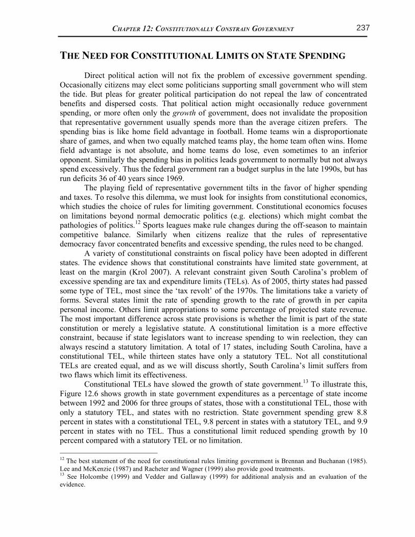
12
and not bottled water at the grocery store, you will come home with soft drinks. We can decide what career to pursue, or if we want to start a business, even though we cannot guarantee ourselves success. In politics you can vote or volunteer or contribute money to your favorite candidate or cause, yet still end up with the other outcome. In politics, our actions rarely determine outcomes: your vote only actually decides a tie election, and elections almost never end in ties. The weak correlation between action and outcomes gives people little reason to participate in politics – why take time off work to go stand in line if your vote is unlikely to matter? This also reduces the incentive for people to become informed about politics – candidates in elections, ballot propositions, and bills under consideration. The lack of incentive to follow politics is known as rational ignorance. The lack of decisiveness also lowers the cost of voting to make a statement without regard to the actual consequences of a policy. Thus people might vote to increase the minimum wage to show that they care about the working poor, even though a higher minimum wage increases unemployment for low wage workers.8 Together the problems of politics create a bias toward excessive spending in representative democracy through the ‘law’ of concentrated benefits and dispersed costs.9 Agenda control creates the ability for politicians to pursue policies benefitting themselves or interest groups, and infrequent elections are a weak device to prevent such manipulation. Bureaucrats and government employees will favor increased spending which leads to higher salaries, larger staffs, greater prestige from controlling a larger budget, and additional resources to pursue their mission, and will support representatives who deliver larger budgets.10 Politicians can take credit for government spending to address a problem, like say hiring more police officers to fight crime, building more prisons, or raising teacher salaries. Because of the weak connection between participation and outcomes in politics, only people with a lot at stake tend to follow the issue and get involved. Generally these are the beneficiaries of government spending, as the costs of government spending - higher taxes and reduced disposable income for families - are widely dispersed, and rarely result in press conferences or photo opportunities. For example, there are about 70,000 full-time public school (K-12) teachers in South Carolina, and about 1.77 million households in the state. If the state government appropriated funds to give each teacher a $5,000 per year raise, the cost per household would be about $200 per year. Two hundred dollars is not a trivial sum, but the average teacher has much more at stake than the average taxpayer. So it is not surprising that teachers and not taxpayers rally at the state capitol when the legislature considers school funding. Powerful teachers unions will lobby and make campaign contributions to support legislators’ votes to increase spending on public schools.11 Politicians will find that voting for increased spending brings them benefits.
8 Brennan and Lomasky (1993) call this type of voting “expressive voting” and analyze such incentives in
democracy. See also Caplan (2007) on how the lack of decisiveness can have far-ranging effects on voters’ political world views. 9 Buchanan and Wagner (1977) offer an excellent dissection of democratic politics’ pro-spending bias. 10 Niskanen (1971) analyzes the pro-spending bias of government bureaucracy. 11 For a discussion of how these forces over time affect representatives and generate a “Culture of Spending,”
see Payne (1991).
13
THE NEED FOR CONSTITUTIONAL LIMITS ON STATE SPENDING
Direct political action will not fix the problem of excessive government spending. Occasionally citizens may elect some politicians supporting small government who will stem the tide. But pleas for greater political participation do not repeal the law of concentrated benefits and dispersed costs. That political action might occasionally reduce government spending, or more often only the growth of government, does not invalidate the proposition that representative government usually spends more than the average citizen prefers. The spending bias is like home field advantage in football. Home teams win a disproportionate share of games, and when two equally matched teams play, the home team often wins. Home field advantage is not absolute, and home teams do lose, even sometimes to an inferior opponent. Similarly the spending bias in politics leads government to normally but not always spend excessively. Thus the federal government ran a budget surplus in the late 1990s, but has run deficits 36 of 40 years since 1969. The playing field of representative government tilts in the favor of higher spending and taxes. To resolve this dilemma, we must look for insights from constitutional economics, which studies the choice of rules for limiting government. Constitutional economics focuses on limitations beyond normal democratic politics (e.g. elections) which might combat the pathologies of politics.12 Sports leagues make rule changes during the off-season to maintain competitive balance. Similarly when citizens realize that the rules of representative democracy favor concentrated benefits and excessive spending, the rules need to be changed. A variety of constitutional constraints on fiscal policy have been adopted in different states. The evidence shows that constitutional constraints have limited state government, at least on the margin (Krol 2007). A relevant constraint given South Carolina’s problem of excessive spending are tax and expenditure limits (TELs). As of 2005, thirty states had passed some type of TEL, most since the ‘tax revolt’ of the 1970s. The limitations take a variety of forms. Several states limit the rate of spending growth to the rate of growth in per capita personal income. Others limit appropriations to some percentage of projected state revenue. The most important difference across state provisions is whether the limit is part of the state constitution or merely a legislative statute. A constitutional limitation is a more effective constraint, because if state legislators want to increase spending to win reelection, they can always rescind a statutory limitation. A total of 17 states, including South Carolina, have a constitutional TEL, while thirteen states have only a statutory TEL. Not all constitutional TELs are created equal, and as we will discuss shortly, South Carolina’s limit suffers from two flaws which limit its effectiveness. Constitutional TELs have slowed the growth of state government.13 To illustrate this, Figure 12.6 shows growth in state government expenditures as a percentage of state income between 1992 and 2006 for three groups of states, those with a constitutional TEL, those with only a statutory TEL, and states with no restriction. State government spending grew 8.8 percent in states with a constitutional TEL, 9.8 percent in states with a statutory TEL, and 9.9 percent in states with no TEL. Thus a constitutional limit reduced spending growth by 10 percent compared with a statutory TEL or no limitation.
12 The best statement of the need for constitutional rules limiting government is Brennan and Buchanan (1985).
Lee and McKenzie (1987) and Racheter and Wagner (1999) also provide good treatments. 13 See Holcombe (1999) and Vedder and Gallaway (1999) for additional analysis and an evaluation of the
evidence.
Chapter 12: Constitutionally Constrain governmentUNLEASHING CAPITALISM 18
manufacturing property tax in the country. In Figure 5.8 we present the effective property tax rates data for Southeastern states, for comparison. The ranks given for the states are out of all 50 states. The ‘net tax’ and ‘effective tax rate’ are calculated based on property valued at $25 million ($12.5 million in machinery and equipment, $12.5 million in inventories, and $2.5 million in fixtures). Notice that South Carolina’s effective tax rate on industrial property is over 7.8 times higher than the most industry-friendly state, Delaware. (Delaware is listed in the figure because it is the lowest-tax state.)
Figure 5.8: Industrial Property Taxes in Southeastern states*, 2007 State Rank (of 50) Net Tax Effective Tax Rate
South Carolina 1 $1,864,900 3.73%
Mississippi 4 $1,291,050 2.58%
Texas 6 $1,264,358 2.53%
Tennessee 10 $1,033,544 2.07%
West Virginia 14 $833,234 1.67%
Louisiana 17 $783,407 1.57%
Georgia 20 $760,381 1.52%
Florida 24 $677,683 1.36%
Alabama 35 $533,776 1.11%
North Carolina 37 $491,071 0.98%
Kentucky 47 $327,100 0.65%
Virginia 49 $241,498 0.48%
Delaware 50 $238,840 0.48%
Source: National Association of Manufacturers (2009) * Taxes measured in the states’ largest city only.
Importantly, South Carolina’s effective tax rate is almost 2.5 times greater than Georgia’s tax, and almost 4 times greater than North Carolina’s. This puts South Carolina at a serious disadvantage, in terms of its ability to attract and keep industry. Since South Carolina has the highest tax in the country on industrial property, it should be no surprise that it has one of the lowest per capita incomes and economic growth rates in the country. Although it is probably not critical that South Carolina set its tax rate to the lowest in the country, it should definitely make it at least competitive for the Southeast. Since Georgia’s rate is effectively 1.52 percent and North Carolina’s is just under 1 percent, a rate at around 1 percent might be sufficient to attract more industry. Working to reduce the various taxes applied to industry would seriously improve the state’s competitiveness. Such a significant reduction in taxes on industrial property would obviously lead to a reduction in tax revenues on industrial property, at least initially. However, the overall revenue may in fact increase once the growth rate in the state begins to pick up and more industry moves into the state. Furthermore, if the official tax rates are lowered, then the state
237CHAPTER 5: SPECIFIC TAX REFORMS
13
Presumably the original intent of imposing a tax rate schedule with graduated marginal tax rates was to make the income tax progressive. However, what progressivity exists in the state’s income tax structure is due to the zero tax on the first $2,630 of income, and because of the graduated marginal tax rates. However, since the marginal tax rate increases over such small steps in income, as shown in Figure 5.5, most of the progressivity occurs at lower income levels, not higher levels of income. At higher income levels, the average tax rate hardly increases at all. This nature of the current tax is directly contradictory to the goal of progressivity. So although on the surface it appears that the tax satisfies the vertical equity condition, it really does this only at the lower income levels reducing the wealth of these lowest income taxpayers, not the intended consequence.
Figure 5.5: South Carolina income tax: Current tax rates compared to inflation-indexed rates, 2009
Current Income Tax
Rates/Brackets
Income Tax Rates/Brackets if 1959 Tax Schedule was Inflation Adjusted to
2009
Taxable Income Tax
Amount Average Tax Rate
Tax Amount
Average Tax Rate
$5,000 $71 1.42% $125 2.5%
$10,000 $290 2.90% $250 2.5%
$15,000 $604 4.03% $377 2.51%
$20,000 $954 4.77% $527 2.63%
$30,000 $1,654 5.51% $834 2.78%
$50,000 $3,054 6.10% $1,695 3.39%
$75,000 $4,804 6.41% $3,127 4.17%
$100,000 $6,554 6.56% $4,877 4.88%
$150,000 $10,054 6.70% $8,377 5.58%
$200,000 $13,554 6.77% $11,877 5.94%
Figure 5.5 also shows what the average tax rates are for various incomes and taxes
under the current tax system in South Carolina. In the right columns it also shows what the taxes and average tax rates would be if the 1959 tax tables were indexed for inflation. The figure clearly shows that the 1959 indexed tax rate structure is more uniformly progressive, especially at higher levels of incomes. It keeps tax rates extremely low for the lowest income individuals in the state. Figure 5.5 also shows that the current tax system charges all income groups more in taxes than an indexed rate schedule. The only exception is the $5,000 income earner in the table. As South Carolina income taxes continue to climb while the tax brackets remain stagnant, the state becomes a relatively high-tax state. This has a negative impact on
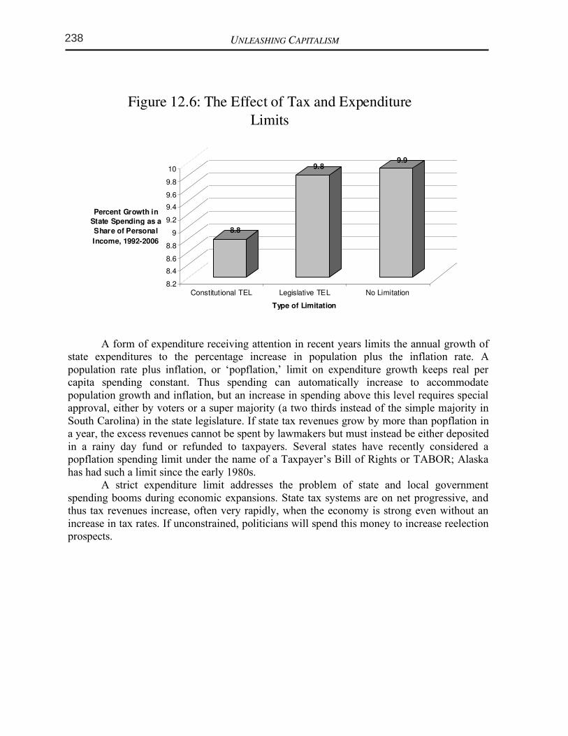
14
8.8
9.89.9
8.2
8.4
8.6
8.8
9
9.2
9.4
9.6
9.8
10
Percent Growth in
State Spending as
a Share of
Personal Income,
1992-2006
Constitutional TEL Legislative TEL No Limitation
Type of Limitation
Figure 12.6: The Effect of Tax and Expenditure
Limits
A form of expenditure receiving attention in recent years limits the annual growth of state expenditures to the percentage increase in population plus the inflation rate. A population rate plus inflation, or ‘popflation,’ limit on expenditure growth keeps real per capita spending constant. Thus spending can automatically increase to accommodate population growth and inflation, but an increase in spending above this level requires special approval, either by voters or a super majority (a two thirds instead of the simple majority in South Carolina) in the state legislature. If state tax revenues grow by more than popflation in a year, the excess revenues cannot be spent by lawmakers but must instead be either deposited in a rainy day fund or refunded to taxpayers. Several states have recently considered a popflation spending limit under the name of a Taxpayer’s Bill of Rights or TABOR; Alaska has had such a limit since the early 1980s. A strict expenditure limit addresses the problem of state and local government spending booms during economic expansions. State tax systems are on net progressive, and thus tax revenues increase, often very rapidly, when the economy is strong even without an increase in tax rates. If unconstrained, politicians will spend this money to increase reelection prospects.
15
Figure 12.7: State Spending Growth in South Carolina
0
5
10
15
20
25
30
1992
1993
1994
1995
1996
1997
1998
1999
2000
2001
2002
2003
2004
2005
2006
2007
Spendin
g
(in
Billions
of
Dollars
)
Actual Spending
Popflation Spending
Figure 12.7 reflects this problem in South Carolina, showing the growth to total state expenditures over 1992-2007. The figure graphs both actual spending and the popflation in the state. Over the period state spending grew about 40 percent more than the popflation value, and most of this excess spending occurred between 1997 and 2002. Such spending sprees result in two problems. First, the new spending is often for pork barrel projects of questionable value. After all, state and local government were already supplying important services like roads, police, courts, and prisons before the boom. Flush coffers allow politicians to fund wasteful projects that nonetheless win votes due to the law of concentrated benefits. In South Carolina, areas of state spending which increased the most proportionally over 1997-2002 included highways, welfare and government administration. Limiting the pork barrel spending spree will result in a better use of resources. Second, when the economy eventually goes into recession and tax revenues fall, states face a budget crisis, made worse by the spending boom. States often engage in unsustainable spending, hiring new employees and beginning new programs requiring funding even when revenues fall. The fiscal crises that states confront with each recession are due primarily to excess spending booms, not inadequate revenue to fund core government services (Stansel and Mitchell 2008). Politicians often then manipulate a budget crisis to their advantage, exploiting agenda setting power to threaten to cut vital services instead of the new pork barrel spending if tax increases are not approved.14 For instance, states which faced worse fiscal crises during the 1990-91 recession were more likely to raise taxes, and then recovered from the recession more slowly (Poterba 1994). The tax hikes diminish economic freedom and set the stage for another cycle of excess spending when the economy recovers. A strict expenditure limit can help end this spending spree, budget crisis cycle once and for all. Limiting the growth of government spending during a boom is likely to be easier politically than cutting existing programs. Before new spending is approved, no one knows exactly who will benefit from the new programs – who will be hired for new jobs, what
14 Mitchell and Simmons (1994) label this the Washington Monument strategy after the Federal government’s
closing of national parks during the government shutdown in 1995. Similarly school boards will threaten to cut
bus service or athletics or even close schools before the end of the year in advance of a school millage election
instead of laying off administrators.
UNLEASHING CAPITALISM 18
manufacturing property tax in the country. In Figure 5.8 we present the effective property tax rates data for Southeastern states, for comparison. The ranks given for the states are out of all 50 states. The ‘net tax’ and ‘effective tax rate’ are calculated based on property valued at $25 million ($12.5 million in machinery and equipment, $12.5 million in inventories, and $2.5 million in fixtures). Notice that South Carolina’s effective tax rate on industrial property is over 7.8 times higher than the most industry-friendly state, Delaware. (Delaware is listed in the figure because it is the lowest-tax state.)
Figure 5.8: Industrial Property Taxes in Southeastern states*, 2007 State Rank (of 50) Net Tax Effective Tax Rate
South Carolina 1 $1,864,900 3.73%
Mississippi 4 $1,291,050 2.58%
Texas 6 $1,264,358 2.53%
Tennessee 10 $1,033,544 2.07%
West Virginia 14 $833,234 1.67%
Louisiana 17 $783,407 1.57%
Georgia 20 $760,381 1.52%
Florida 24 $677,683 1.36%
Alabama 35 $533,776 1.11%
North Carolina 37 $491,071 0.98%
Kentucky 47 $327,100 0.65%
Virginia 49 $241,498 0.48%
Delaware 50 $238,840 0.48%
Source: National Association of Manufacturers (2009) * Taxes measured in the states’ largest city only.
Importantly, South Carolina’s effective tax rate is almost 2.5 times greater than Georgia’s tax, and almost 4 times greater than North Carolina’s. This puts South Carolina at a serious disadvantage, in terms of its ability to attract and keep industry. Since South Carolina has the highest tax in the country on industrial property, it should be no surprise that it has one of the lowest per capita incomes and economic growth rates in the country. Although it is probably not critical that South Carolina set its tax rate to the lowest in the country, it should definitely make it at least competitive for the Southeast. Since Georgia’s rate is effectively 1.52 percent and North Carolina’s is just under 1 percent, a rate at around 1 percent might be sufficient to attract more industry. Working to reduce the various taxes applied to industry would seriously improve the state’s competitiveness. Such a significant reduction in taxes on industrial property would obviously lead to a reduction in tax revenues on industrial property, at least initially. However, the overall revenue may in fact increase once the growth rate in the state begins to pick up and more industry moves into the state. Furthermore, if the official tax rates are lowered, then the state
8.8
9.89.9
8.2
8.4
8.6
8.8
9
9.2
9.4
9.6
9.8
10
Percent Growth in
State Spending as a
Share of Personal
Income, 1992-2006
Constitutional TEL Legislative TEL No Limitation
Type of Limitation
Figure 12.6: The Effect of Tax and Expenditure
Limits
UNLEASHING CAPITALISM 18
manufacturing property tax in the country. In Figure 5.8 we present the effective property tax rates data for Southeastern states, for comparison. The ranks given for the states are out of all 50 states. The ‘net tax’ and ‘effective tax rate’ are calculated based on property valued at $25 million ($12.5 million in machinery and equipment, $12.5 million in inventories, and $2.5 million in fixtures). Notice that South Carolina’s effective tax rate on industrial property is over 7.8 times higher than the most industry-friendly state, Delaware. (Delaware is listed in the figure because it is the lowest-tax state.)
Figure 5.8: Industrial Property Taxes in Southeastern states*, 2007 State Rank (of 50) Net Tax Effective Tax Rate
South Carolina 1 $1,864,900 3.73%
Mississippi 4 $1,291,050 2.58%
Texas 6 $1,264,358 2.53%
Tennessee 10 $1,033,544 2.07%
West Virginia 14 $833,234 1.67%
Louisiana 17 $783,407 1.57%
Georgia 20 $760,381 1.52%
Florida 24 $677,683 1.36%
Alabama 35 $533,776 1.11%
North Carolina 37 $491,071 0.98%
Kentucky 47 $327,100 0.65%
Virginia 49 $241,498 0.48%
Delaware 50 $238,840 0.48%
Source: National Association of Manufacturers (2009) * Taxes measured in the states’ largest city only.
Importantly, South Carolina’s effective tax rate is almost 2.5 times greater than Georgia’s tax, and almost 4 times greater than North Carolina’s. This puts South Carolina at a serious disadvantage, in terms of its ability to attract and keep industry. Since South Carolina has the highest tax in the country on industrial property, it should be no surprise that it has one of the lowest per capita incomes and economic growth rates in the country. Although it is probably not critical that South Carolina set its tax rate to the lowest in the country, it should definitely make it at least competitive for the Southeast. Since Georgia’s rate is effectively 1.52 percent and North Carolina’s is just under 1 percent, a rate at around 1 percent might be sufficient to attract more industry. Working to reduce the various taxes applied to industry would seriously improve the state’s competitiveness. Such a significant reduction in taxes on industrial property would obviously lead to a reduction in tax revenues on industrial property, at least initially. However, the overall revenue may in fact increase once the growth rate in the state begins to pick up and more industry moves into the state. Furthermore, if the official tax rates are lowered, then the state
238 CHAPTER 5: SPECIFIC TAX REFORMS
13
Presumably the original intent of imposing a tax rate schedule with graduated marginal tax rates was to make the income tax progressive. However, what progressivity exists in the state’s income tax structure is due to the zero tax on the first $2,630 of income, and because of the graduated marginal tax rates. However, since the marginal tax rate increases over such small steps in income, as shown in Figure 5.5, most of the progressivity occurs at lower income levels, not higher levels of income. At higher income levels, the average tax rate hardly increases at all. This nature of the current tax is directly contradictory to the goal of progressivity. So although on the surface it appears that the tax satisfies the vertical equity condition, it really does this only at the lower income levels reducing the wealth of these lowest income taxpayers, not the intended consequence.
Figure 5.5: South Carolina income tax: Current tax rates compared to inflation-indexed rates, 2009
Current Income Tax
Rates/Brackets
Income Tax Rates/Brackets if 1959 Tax Schedule was Inflation Adjusted to
2009
Taxable Income Tax
Amount Average Tax Rate
Tax Amount
Average Tax Rate
$5,000 $71 1.42% $125 2.5%
$10,000 $290 2.90% $250 2.5%
$15,000 $604 4.03% $377 2.51%
$20,000 $954 4.77% $527 2.63%
$30,000 $1,654 5.51% $834 2.78%
$50,000 $3,054 6.10% $1,695 3.39%
$75,000 $4,804 6.41% $3,127 4.17%
$100,000 $6,554 6.56% $4,877 4.88%
$150,000 $10,054 6.70% $8,377 5.58%
$200,000 $13,554 6.77% $11,877 5.94%
Figure 5.5 also shows what the average tax rates are for various incomes and taxes
under the current tax system in South Carolina. In the right columns it also shows what the taxes and average tax rates would be if the 1959 tax tables were indexed for inflation. The figure clearly shows that the 1959 indexed tax rate structure is more uniformly progressive, especially at higher levels of incomes. It keeps tax rates extremely low for the lowest income individuals in the state. Figure 5.5 also shows that the current tax system charges all income groups more in taxes than an indexed rate schedule. The only exception is the $5,000 income earner in the table. As South Carolina income taxes continue to climb while the tax brackets remain stagnant, the state becomes a relatively high-tax state. This has a negative impact on
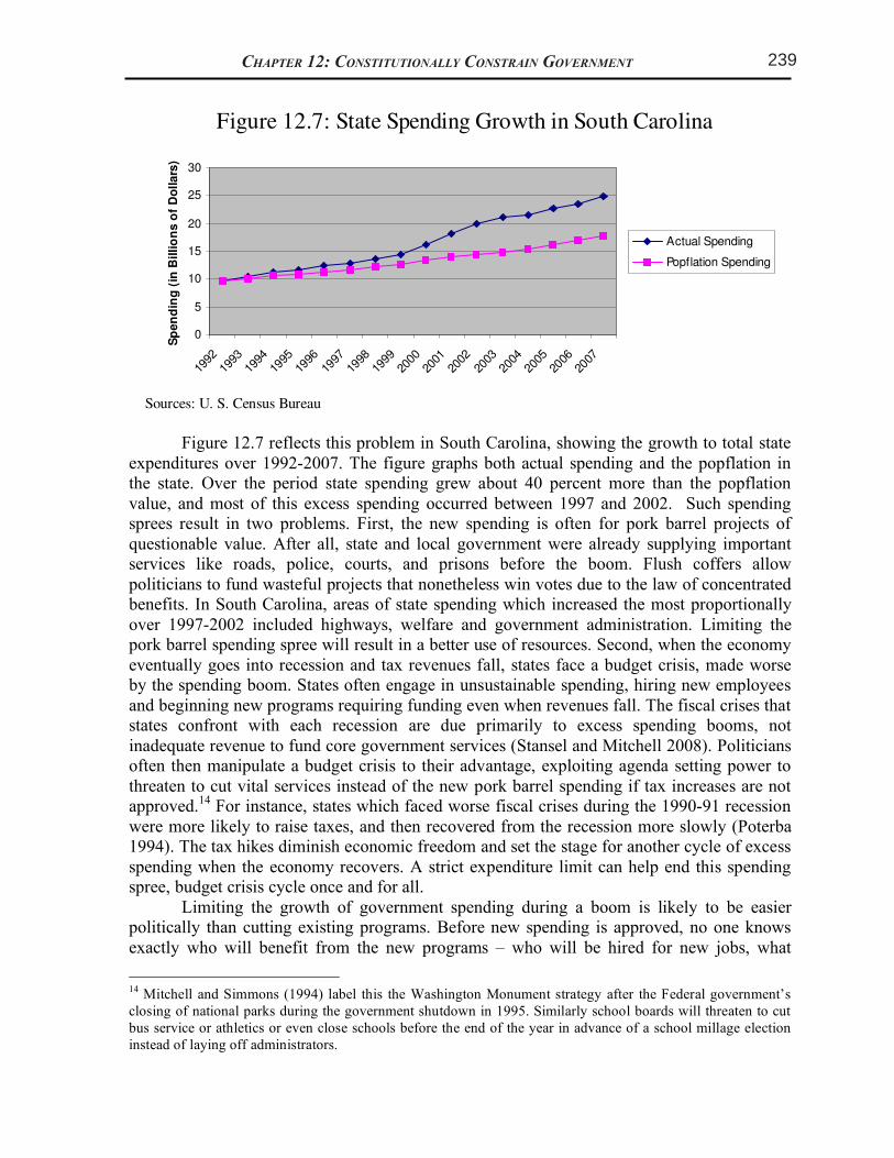
14
8.8
9.89.9
8.2
8.4
8.6
8.8
9
9.2
9.4
9.6
9.8
10
Percent Growth in
State Spending as
a Share of
Personal Income,
1992-2006
Constitutional TEL Legislative TEL No Limitation
Type of Limitation
Figure 12.6: The Effect of Tax and Expenditure
Limits
A form of expenditure receiving attention in recent years limits the annual growth of state expenditures to the percentage increase in population plus the inflation rate. A population rate plus inflation, or ‘popflation,’ limit on expenditure growth keeps real per capita spending constant. Thus spending can automatically increase to accommodate population growth and inflation, but an increase in spending above this level requires special approval, either by voters or a super majority (a two thirds instead of the simple majority in South Carolina) in the state legislature. If state tax revenues grow by more than popflation in a year, the excess revenues cannot be spent by lawmakers but must instead be either deposited in a rainy day fund or refunded to taxpayers. Several states have recently considered a popflation spending limit under the name of a Taxpayer’s Bill of Rights or TABOR; Alaska has had such a limit since the early 1980s. A strict expenditure limit addresses the problem of state and local government spending booms during economic expansions. State tax systems are on net progressive, and thus tax revenues increase, often very rapidly, when the economy is strong even without an increase in tax rates. If unconstrained, politicians will spend this money to increase reelection prospects.
15
Figure 12.7: State Spending Growth in South Carolina
0
5
10
15
20
25
30
1992
1993
1994
1995
1996
1997
1998
1999
2000
2001
2002
2003
2004
2005
2006
2007
Spendin
g
(in
Billions
of
Dollars
)
Actual Spending
Popflation Spending
Figure 12.7 reflects this problem in South Carolina, showing the growth to total state expenditures over 1992-2007. The figure graphs both actual spending and the popflation in the state. Over the period state spending grew about 40 percent more than the popflation value, and most of this excess spending occurred between 1997 and 2002. Such spending sprees result in two problems. First, the new spending is often for pork barrel projects of questionable value. After all, state and local government were already supplying important services like roads, police, courts, and prisons before the boom. Flush coffers allow politicians to fund wasteful projects that nonetheless win votes due to the law of concentrated benefits. In South Carolina, areas of state spending which increased the most proportionally over 1997-2002 included highways, welfare and government administration. Limiting the pork barrel spending spree will result in a better use of resources. Second, when the economy eventually goes into recession and tax revenues fall, states face a budget crisis, made worse by the spending boom. States often engage in unsustainable spending, hiring new employees and beginning new programs requiring funding even when revenues fall. The fiscal crises that states confront with each recession are due primarily to excess spending booms, not inadequate revenue to fund core government services (Stansel and Mitchell 2008). Politicians often then manipulate a budget crisis to their advantage, exploiting agenda setting power to threaten to cut vital services instead of the new pork barrel spending if tax increases are not approved.14 For instance, states which faced worse fiscal crises during the 1990-91 recession were more likely to raise taxes, and then recovered from the recession more slowly (Poterba 1994). The tax hikes diminish economic freedom and set the stage for another cycle of excess spending when the economy recovers. A strict expenditure limit can help end this spending spree, budget crisis cycle once and for all. Limiting the growth of government spending during a boom is likely to be easier politically than cutting existing programs. Before new spending is approved, no one knows exactly who will benefit from the new programs – who will be hired for new jobs, what
14 Mitchell and Simmons (1994) label this the Washington Monument strategy after the Federal government’s
closing of national parks during the government shutdown in 1995. Similarly school boards will threaten to cut
bus service or athletics or even close schools before the end of the year in advance of a school millage election
instead of laying off administrators.
Chapter 12: Constitutionally Constrain government
Figure 12.7: State Spending Growth in South Carolina
0
5
10
15
20
25
30
1992
1993
1994
1995
1996
1997
1998
1999
2000
2001
2002
2003
2004
2005
2006
2007
Sp
en
din
g (
in B
illio
ns o
f D
ollars
)
Actual Spending
Popflation Spending
Sources: U. S. Census Bureau
UNLEASHING CAPITALISM 18
manufacturing property tax in the country. In Figure 5.8 we present the effective property tax rates data for Southeastern states, for comparison. The ranks given for the states are out of all 50 states. The ‘net tax’ and ‘effective tax rate’ are calculated based on property valued at $25 million ($12.5 million in machinery and equipment, $12.5 million in inventories, and $2.5 million in fixtures). Notice that South Carolina’s effective tax rate on industrial property is over 7.8 times higher than the most industry-friendly state, Delaware. (Delaware is listed in the figure because it is the lowest-tax state.)
Figure 5.8: Industrial Property Taxes in Southeastern states*, 2007 State Rank (of 50) Net Tax Effective Tax Rate
South Carolina 1 $1,864,900 3.73%
Mississippi 4 $1,291,050 2.58%
Texas 6 $1,264,358 2.53%
Tennessee 10 $1,033,544 2.07%
West Virginia 14 $833,234 1.67%
Louisiana 17 $783,407 1.57%
Georgia 20 $760,381 1.52%
Florida 24 $677,683 1.36%
Alabama 35 $533,776 1.11%
North Carolina 37 $491,071 0.98%
Kentucky 47 $327,100 0.65%
Virginia 49 $241,498 0.48%
Delaware 50 $238,840 0.48%
Source: National Association of Manufacturers (2009) * Taxes measured in the states’ largest city only.
Importantly, South Carolina’s effective tax rate is almost 2.5 times greater than Georgia’s tax, and almost 4 times greater than North Carolina’s. This puts South Carolina at a serious disadvantage, in terms of its ability to attract and keep industry. Since South Carolina has the highest tax in the country on industrial property, it should be no surprise that it has one of the lowest per capita incomes and economic growth rates in the country. Although it is probably not critical that South Carolina set its tax rate to the lowest in the country, it should definitely make it at least competitive for the Southeast. Since Georgia’s rate is effectively 1.52 percent and North Carolina’s is just under 1 percent, a rate at around 1 percent might be sufficient to attract more industry. Working to reduce the various taxes applied to industry would seriously improve the state’s competitiveness. Such a significant reduction in taxes on industrial property would obviously lead to a reduction in tax revenues on industrial property, at least initially. However, the overall revenue may in fact increase once the growth rate in the state begins to pick up and more industry moves into the state. Furthermore, if the official tax rates are lowered, then the state
239CHAPTER 5: SPECIFIC TAX REFORMS
13
Presumably the original intent of imposing a tax rate schedule with graduated marginal tax rates was to make the income tax progressive. However, what progressivity exists in the state’s income tax structure is due to the zero tax on the first $2,630 of income, and because of the graduated marginal tax rates. However, since the marginal tax rate increases over such small steps in income, as shown in Figure 5.5, most of the progressivity occurs at lower income levels, not higher levels of income. At higher income levels, the average tax rate hardly increases at all. This nature of the current tax is directly contradictory to the goal of progressivity. So although on the surface it appears that the tax satisfies the vertical equity condition, it really does this only at the lower income levels reducing the wealth of these lowest income taxpayers, not the intended consequence.
Figure 5.5: South Carolina income tax: Current tax rates compared to inflation-indexed rates, 2009
Current Income Tax
Rates/Brackets
Income Tax Rates/Brackets if 1959 Tax Schedule was Inflation Adjusted to
2009
Taxable Income Tax
Amount Average Tax Rate
Tax Amount
Average Tax Rate
$5,000 $71 1.42% $125 2.5%
$10,000 $290 2.90% $250 2.5%
$15,000 $604 4.03% $377 2.51%
$20,000 $954 4.77% $527 2.63%
$30,000 $1,654 5.51% $834 2.78%
$50,000 $3,054 6.10% $1,695 3.39%
$75,000 $4,804 6.41% $3,127 4.17%
$100,000 $6,554 6.56% $4,877 4.88%
$150,000 $10,054 6.70% $8,377 5.58%
$200,000 $13,554 6.77% $11,877 5.94%
Figure 5.5 also shows what the average tax rates are for various incomes and taxes
under the current tax system in South Carolina. In the right columns it also shows what the taxes and average tax rates would be if the 1959 tax tables were indexed for inflation. The figure clearly shows that the 1959 indexed tax rate structure is more uniformly progressive, especially at higher levels of incomes. It keeps tax rates extremely low for the lowest income individuals in the state. Figure 5.5 also shows that the current tax system charges all income groups more in taxes than an indexed rate schedule. The only exception is the $5,000 income earner in the table. As South Carolina income taxes continue to climb while the tax brackets remain stagnant, the state becomes a relatively high-tax state. This has a negative impact on
16
companies will get contracts – is not yet known. Consequently we do not have individuals who face the loss of their jobs or reduction in income as when spending is reduced. Over time the effect of avoiding excessive spending can be extensive. Spending in South Carolina was 40 percent greater in 2007 than it would have been if held to the popflation level since 1992 (see Figure 12.7). Cutting state government spending by 30 percent now would likely be a Herculean task, but the same effect could have been achieved merely by limiting spending since 1992. Figure 12.7 considers the potential benefits of limiting excess spending during booms. For each state, we take state and local spending in 1992 and adjust for state population growth and national inflation between 1992 and 2006. We then divided actual state spending in 2006 by the popflation limited level, creating a ratio of excess spending over the period. A ratio of 1, for example, means that state spending was at the level it would have been under a popflation rule while a ratio of 2 means that actual spending was double the popflation limit level. Figure 12.8 then graphs the scatterplot of state income against our index of excess spending. States indulging in spending sprees were poorer in 2006. And the consequence of excessive spending is dramatic. The trend line shows that an excess spending ratio of 2 compared to 1 is associated with about 25 percent lower PCPI in 2006.
Figure 12.8: Spending Growth in Excess of
Popflation and State Income
0
10
20
30
40
50
60
0 0.2 0.4 0.6 0.8 1 1.2 1.4 1.6 1.8 2
Index of Excess Spending, 1992-2006
Per
Capit
a
Pers
onal
Incom
e,
20
06
South Carolina currently has a constitutional TEL in place, and yet has experienced reasonably fast growth in state spending. The state’s excess spending ratio for 1992-2006 was 1.41, exceeding the average across states of 1.36. South Carolina’s expenditure limitation suffers from two weaknesses (Poulson 2005). First, the limit in the state’s TEL is relatively high, at over 9 percent of state income, so although TELs cap annual expenditure growth, the cap in South Carolina is too high. Second, the South Carolina limitation requires that excess revenues either be placed in a rainy day fund or can be used to attract federal matching funds. Rainy day funds are problematic as a limit on government; Wagner and Sobel (2006) show that these funds can be used by legislators to circumvent spending limits. A preferable limit would return revenues in excess of a much stricter limit to taxpayers each year.
17
DECENTRALIZATION AND SEPARATION OF POWERS
Most of the time people debate whether government should provide a service, but
which level of government should undertake a task is also an important question. The U.S. features multiple levels of government, with the Federal government, the fifty state governments, county and city governments, and independent governmental units like school and water districts. Government in South Carolina is currently relatively centralized, and the state could benefit from decentralizing its government. A guiding principle for assigning functions to different levels of government is to match the geographic scope of the benefits of government goods and services with political jurisdictions. A strong military defends an entire country, so defense is naturally a national government function, while parks and street repairs primarily benefit local residents and thus are an appropriate municipal government function. A well-designed system of fiscal federalism benefits society in several ways, perhaps most importantly by accommodating people’s differing preferences for government goods and services. Where state government might adopt a one-size-fits-all approach, local communities can choose a combination of spending on parks, police, schools and other services that reflects the preferences of their residents. When cities make these decisions, local residents can choose to spend more on the services they desire. Of course, the problems of politics might lead to a bias toward excessive spending by local governments, but when local government provides services, citizens now have an additional mechanism to limit spending: they can ‘vote with their feet’ and leave a community which spends too much. Charles Tiebout (1956) proposed that mobility across communities lets citizens choose local government services in a manner analogous to the market place. If people move to communities with low crime rates and excellent parks, this lets politicians know that people value these government services, as opposed to say smaller class sizes in public schools. Local government should be more responsive to citizen preferences. Albert Hirschman (1970) explains how political participation, or ‘voice,’ and voting with one’s feet, or ‘exit,’ interact in controlling organizations, including government. Both exit and voice operate more effectively at the local level than at the state level. Political action by any one individual is more likely to be decisive in a small community, making voice more effective. In addition, exit is more effective because moving to the next town is less disruptive than moving to another state.
UNLEASHING CAPITALISM 18
manufacturing property tax in the country. In Figure 5.8 we present the effective property tax rates data for Southeastern states, for comparison. The ranks given for the states are out of all 50 states. The ‘net tax’ and ‘effective tax rate’ are calculated based on property valued at $25 million ($12.5 million in machinery and equipment, $12.5 million in inventories, and $2.5 million in fixtures). Notice that South Carolina’s effective tax rate on industrial property is over 7.8 times higher than the most industry-friendly state, Delaware. (Delaware is listed in the figure because it is the lowest-tax state.)
Figure 5.8: Industrial Property Taxes in Southeastern states*, 2007 State Rank (of 50) Net Tax Effective Tax Rate
South Carolina 1 $1,864,900 3.73%
Mississippi 4 $1,291,050 2.58%
Texas 6 $1,264,358 2.53%
Tennessee 10 $1,033,544 2.07%
West Virginia 14 $833,234 1.67%
Louisiana 17 $783,407 1.57%
Georgia 20 $760,381 1.52%
Florida 24 $677,683 1.36%
Alabama 35 $533,776 1.11%
North Carolina 37 $491,071 0.98%
Kentucky 47 $327,100 0.65%
Virginia 49 $241,498 0.48%
Delaware 50 $238,840 0.48%
Source: National Association of Manufacturers (2009) * Taxes measured in the states’ largest city only.
Importantly, South Carolina’s effective tax rate is almost 2.5 times greater than Georgia’s tax, and almost 4 times greater than North Carolina’s. This puts South Carolina at a serious disadvantage, in terms of its ability to attract and keep industry. Since South Carolina has the highest tax in the country on industrial property, it should be no surprise that it has one of the lowest per capita incomes and economic growth rates in the country. Although it is probably not critical that South Carolina set its tax rate to the lowest in the country, it should definitely make it at least competitive for the Southeast. Since Georgia’s rate is effectively 1.52 percent and North Carolina’s is just under 1 percent, a rate at around 1 percent might be sufficient to attract more industry. Working to reduce the various taxes applied to industry would seriously improve the state’s competitiveness. Such a significant reduction in taxes on industrial property would obviously lead to a reduction in tax revenues on industrial property, at least initially. However, the overall revenue may in fact increase once the growth rate in the state begins to pick up and more industry moves into the state. Furthermore, if the official tax rates are lowered, then the state
Figure 12.8: Spending Growth in Excess of
Popflation and State Income
0
10
20
30
40
50
60
0 0.2 0.4 0.6 0.8 1 1.2 1.4 1.6 1.8 2
Index of Excess Spending, 1992-2006
Pe
r C
ap
ita
Pe
rso
na
l In
co
me
,
20
06
UNLEASHING CAPITALISM 18
manufacturing property tax in the country. In Figure 5.8 we present the effective property tax rates data for Southeastern states, for comparison. The ranks given for the states are out of all 50 states. The ‘net tax’ and ‘effective tax rate’ are calculated based on property valued at $25 million ($12.5 million in machinery and equipment, $12.5 million in inventories, and $2.5 million in fixtures). Notice that South Carolina’s effective tax rate on industrial property is over 7.8 times higher than the most industry-friendly state, Delaware. (Delaware is listed in the figure because it is the lowest-tax state.)
Figure 5.8: Industrial Property Taxes in Southeastern states*, 2007 State Rank (of 50) Net Tax Effective Tax Rate
South Carolina 1 $1,864,900 3.73%
Mississippi 4 $1,291,050 2.58%
Texas 6 $1,264,358 2.53%
Tennessee 10 $1,033,544 2.07%
West Virginia 14 $833,234 1.67%
Louisiana 17 $783,407 1.57%
Georgia 20 $760,381 1.52%
Florida 24 $677,683 1.36%
Alabama 35 $533,776 1.11%
North Carolina 37 $491,071 0.98%
Kentucky 47 $327,100 0.65%
Virginia 49 $241,498 0.48%
Delaware 50 $238,840 0.48%
Source: National Association of Manufacturers (2009) * Taxes measured in the states’ largest city only.
Importantly, South Carolina’s effective tax rate is almost 2.5 times greater than Georgia’s tax, and almost 4 times greater than North Carolina’s. This puts South Carolina at a serious disadvantage, in terms of its ability to attract and keep industry. Since South Carolina has the highest tax in the country on industrial property, it should be no surprise that it has one of the lowest per capita incomes and economic growth rates in the country. Although it is probably not critical that South Carolina set its tax rate to the lowest in the country, it should definitely make it at least competitive for the Southeast. Since Georgia’s rate is effectively 1.52 percent and North Carolina’s is just under 1 percent, a rate at around 1 percent might be sufficient to attract more industry. Working to reduce the various taxes applied to industry would seriously improve the state’s competitiveness. Such a significant reduction in taxes on industrial property would obviously lead to a reduction in tax revenues on industrial property, at least initially. However, the overall revenue may in fact increase once the growth rate in the state begins to pick up and more industry moves into the state. Furthermore, if the official tax rates are lowered, then the state
240 CHAPTER 5: SPECIFIC TAX REFORMS
13
Presumably the original intent of imposing a tax rate schedule with graduated marginal tax rates was to make the income tax progressive. However, what progressivity exists in the state’s income tax structure is due to the zero tax on the first $2,630 of income, and because of the graduated marginal tax rates. However, since the marginal tax rate increases over such small steps in income, as shown in Figure 5.5, most of the progressivity occurs at lower income levels, not higher levels of income. At higher income levels, the average tax rate hardly increases at all. This nature of the current tax is directly contradictory to the goal of progressivity. So although on the surface it appears that the tax satisfies the vertical equity condition, it really does this only at the lower income levels reducing the wealth of these lowest income taxpayers, not the intended consequence.
Figure 5.5: South Carolina income tax: Current tax rates compared to inflation-indexed rates, 2009
Current Income Tax
Rates/Brackets
Income Tax Rates/Brackets if 1959 Tax Schedule was Inflation Adjusted to
2009
Taxable Income Tax
Amount Average Tax Rate
Tax Amount
Average Tax Rate
$5,000 $71 1.42% $125 2.5%
$10,000 $290 2.90% $250 2.5%
$15,000 $604 4.03% $377 2.51%
$20,000 $954 4.77% $527 2.63%
$30,000 $1,654 5.51% $834 2.78%
$50,000 $3,054 6.10% $1,695 3.39%
$75,000 $4,804 6.41% $3,127 4.17%
$100,000 $6,554 6.56% $4,877 4.88%
$150,000 $10,054 6.70% $8,377 5.58%
$200,000 $13,554 6.77% $11,877 5.94%
Figure 5.5 also shows what the average tax rates are for various incomes and taxes
under the current tax system in South Carolina. In the right columns it also shows what the taxes and average tax rates would be if the 1959 tax tables were indexed for inflation. The figure clearly shows that the 1959 indexed tax rate structure is more uniformly progressive, especially at higher levels of incomes. It keeps tax rates extremely low for the lowest income individuals in the state. Figure 5.5 also shows that the current tax system charges all income groups more in taxes than an indexed rate schedule. The only exception is the $5,000 income earner in the table. As South Carolina income taxes continue to climb while the tax brackets remain stagnant, the state becomes a relatively high-tax state. This has a negative impact on
16
companies will get contracts – is not yet known. Consequently we do not have individuals who face the loss of their jobs or reduction in income as when spending is reduced. Over time the effect of avoiding excessive spending can be extensive. Spending in South Carolina was 40 percent greater in 2007 than it would have been if held to the popflation level since 1992 (see Figure 12.7). Cutting state government spending by 30 percent now would likely be a Herculean task, but the same effect could have been achieved merely by limiting spending since 1992. Figure 12.7 considers the potential benefits of limiting excess spending during booms. For each state, we take state and local spending in 1992 and adjust for state population growth and national inflation between 1992 and 2006. We then divided actual state spending in 2006 by the popflation limited level, creating a ratio of excess spending over the period. A ratio of 1, for example, means that state spending was at the level it would have been under a popflation rule while a ratio of 2 means that actual spending was double the popflation limit level. Figure 12.8 then graphs the scatterplot of state income against our index of excess spending. States indulging in spending sprees were poorer in 2006. And the consequence of excessive spending is dramatic. The trend line shows that an excess spending ratio of 2 compared to 1 is associated with about 25 percent lower PCPI in 2006.
Figure 12.8: Spending Growth in Excess of
Popflation and State Income
0
10
20
30
40
50
60
0 0.2 0.4 0.6 0.8 1 1.2 1.4 1.6 1.8 2
Index of Excess Spending, 1992-2006
Per
Capit
a
Pers
onal
Incom
e,
20
06
South Carolina currently has a constitutional TEL in place, and yet has experienced reasonably fast growth in state spending. The state’s excess spending ratio for 1992-2006 was 1.41, exceeding the average across states of 1.36. South Carolina’s expenditure limitation suffers from two weaknesses (Poulson 2005). First, the limit in the state’s TEL is relatively high, at over 9 percent of state income, so although TELs cap annual expenditure growth, the cap in South Carolina is too high. Second, the South Carolina limitation requires that excess revenues either be placed in a rainy day fund or can be used to attract federal matching funds. Rainy day funds are problematic as a limit on government; Wagner and Sobel (2006) show that these funds can be used by legislators to circumvent spending limits. A preferable limit would return revenues in excess of a much stricter limit to taxpayers each year.
17
DECENTRALIZATION AND SEPARATION OF POWERS
Most of the time people debate whether government should provide a service, but
which level of government should undertake a task is also an important question. The U.S. features multiple levels of government, with the Federal government, the fifty state governments, county and city governments, and independent governmental units like school and water districts. Government in South Carolina is currently relatively centralized, and the state could benefit from decentralizing its government. A guiding principle for assigning functions to different levels of government is to match the geographic scope of the benefits of government goods and services with political jurisdictions. A strong military defends an entire country, so defense is naturally a national government function, while parks and street repairs primarily benefit local residents and thus are an appropriate municipal government function. A well-designed system of fiscal federalism benefits society in several ways, perhaps most importantly by accommodating people’s differing preferences for government goods and services. Where state government might adopt a one-size-fits-all approach, local communities can choose a combination of spending on parks, police, schools and other services that reflects the preferences of their residents. When cities make these decisions, local residents can choose to spend more on the services they desire. Of course, the problems of politics might lead to a bias toward excessive spending by local governments, but when local government provides services, citizens now have an additional mechanism to limit spending: they can ‘vote with their feet’ and leave a community which spends too much. Charles Tiebout (1956) proposed that mobility across communities lets citizens choose local government services in a manner analogous to the market place. If people move to communities with low crime rates and excellent parks, this lets politicians know that people value these government services, as opposed to say smaller class sizes in public schools. Local government should be more responsive to citizen preferences. Albert Hirschman (1970) explains how political participation, or ‘voice,’ and voting with one’s feet, or ‘exit,’ interact in controlling organizations, including government. Both exit and voice operate more effectively at the local level than at the state level. Political action by any one individual is more likely to be decisive in a small community, making voice more effective. In addition, exit is more effective because moving to the next town is less disruptive than moving to another state.
Chapter 12: Constitutionally Constrain governmentUNLEASHING CAPITALISM 18
manufacturing property tax in the country. In Figure 5.8 we present the effective property tax rates data for Southeastern states, for comparison. The ranks given for the states are out of all 50 states. The ‘net tax’ and ‘effective tax rate’ are calculated based on property valued at $25 million ($12.5 million in machinery and equipment, $12.5 million in inventories, and $2.5 million in fixtures). Notice that South Carolina’s effective tax rate on industrial property is over 7.8 times higher than the most industry-friendly state, Delaware. (Delaware is listed in the figure because it is the lowest-tax state.)
Figure 5.8: Industrial Property Taxes in Southeastern states*, 2007 State Rank (of 50) Net Tax Effective Tax Rate
South Carolina 1 $1,864,900 3.73%
Mississippi 4 $1,291,050 2.58%
Texas 6 $1,264,358 2.53%
Tennessee 10 $1,033,544 2.07%
West Virginia 14 $833,234 1.67%
Louisiana 17 $783,407 1.57%
Georgia 20 $760,381 1.52%
Florida 24 $677,683 1.36%
Alabama 35 $533,776 1.11%
North Carolina 37 $491,071 0.98%
Kentucky 47 $327,100 0.65%
Virginia 49 $241,498 0.48%
Delaware 50 $238,840 0.48%
Source: National Association of Manufacturers (2009) * Taxes measured in the states’ largest city only.
Importantly, South Carolina’s effective tax rate is almost 2.5 times greater than Georgia’s tax, and almost 4 times greater than North Carolina’s. This puts South Carolina at a serious disadvantage, in terms of its ability to attract and keep industry. Since South Carolina has the highest tax in the country on industrial property, it should be no surprise that it has one of the lowest per capita incomes and economic growth rates in the country. Although it is probably not critical that South Carolina set its tax rate to the lowest in the country, it should definitely make it at least competitive for the Southeast. Since Georgia’s rate is effectively 1.52 percent and North Carolina’s is just under 1 percent, a rate at around 1 percent might be sufficient to attract more industry. Working to reduce the various taxes applied to industry would seriously improve the state’s competitiveness. Such a significant reduction in taxes on industrial property would obviously lead to a reduction in tax revenues on industrial property, at least initially. However, the overall revenue may in fact increase once the growth rate in the state begins to pick up and more industry moves into the state. Furthermore, if the official tax rates are lowered, then the state
241CHAPTER 5: SPECIFIC TAX REFORMS
13
Presumably the original intent of imposing a tax rate schedule with graduated marginal tax rates was to make the income tax progressive. However, what progressivity exists in the state’s income tax structure is due to the zero tax on the first $2,630 of income, and because of the graduated marginal tax rates. However, since the marginal tax rate increases over such small steps in income, as shown in Figure 5.5, most of the progressivity occurs at lower income levels, not higher levels of income. At higher income levels, the average tax rate hardly increases at all. This nature of the current tax is directly contradictory to the goal of progressivity. So although on the surface it appears that the tax satisfies the vertical equity condition, it really does this only at the lower income levels reducing the wealth of these lowest income taxpayers, not the intended consequence.
Figure 5.5: South Carolina income tax: Current tax rates compared to inflation-indexed rates, 2009
Current Income Tax
Rates/Brackets
Income Tax Rates/Brackets if 1959 Tax Schedule was Inflation Adjusted to
2009
Taxable Income Tax
Amount Average Tax Rate
Tax Amount
Average Tax Rate
$5,000 $71 1.42% $125 2.5%
$10,000 $290 2.90% $250 2.5%
$15,000 $604 4.03% $377 2.51%
$20,000 $954 4.77% $527 2.63%
$30,000 $1,654 5.51% $834 2.78%
$50,000 $3,054 6.10% $1,695 3.39%
$75,000 $4,804 6.41% $3,127 4.17%
$100,000 $6,554 6.56% $4,877 4.88%
$150,000 $10,054 6.70% $8,377 5.58%
$200,000 $13,554 6.77% $11,877 5.94%
Figure 5.5 also shows what the average tax rates are for various incomes and taxes
under the current tax system in South Carolina. In the right columns it also shows what the taxes and average tax rates would be if the 1959 tax tables were indexed for inflation. The figure clearly shows that the 1959 indexed tax rate structure is more uniformly progressive, especially at higher levels of incomes. It keeps tax rates extremely low for the lowest income individuals in the state. Figure 5.5 also shows that the current tax system charges all income groups more in taxes than an indexed rate schedule. The only exception is the $5,000 income earner in the table. As South Carolina income taxes continue to climb while the tax brackets remain stagnant, the state becomes a relatively high-tax state. This has a negative impact on
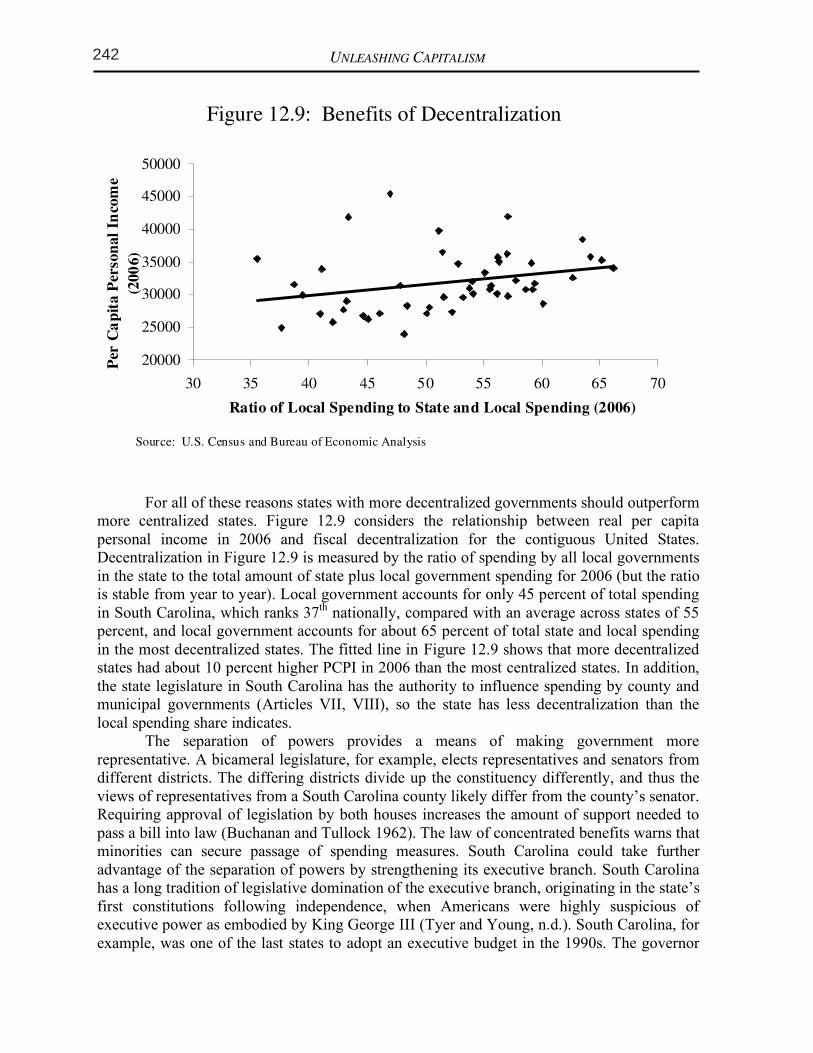
18
Figure 12.9: Benefits of Decentralization
20000
25000
30000
35000
40000
45000
50000
30 35 40 45 50 55 60 65 70
Ratio of Local Spending to State and Local Spending (2006)
Per
Cap
ita P
erso
nal In
com
e (2
006)
Source: U.S. Census and Bureau of Economic Analysis
For all of these reasons states with more decentralized governments should outperform more centralized states. Figure 12.9 considers the relationship between real per capita personal income in 2006 and fiscal decentralization for the contiguous United States. Decentralization in Figure 12.9 is measured by the ratio of spending by all local governments in the state to the total amount of state plus local government spending for 2006 (but the ratio is stable from year to year). Local government accounts for only 45 percent of total spending in South Carolina, which ranks 37th nationally, compared with an average across states of 55 percent, and local government accounts for about 65 percent of total state and local spending in the most decentralized states. The fitted line in Figure 12.9 shows that more decentralized states had about 10 percent higher PCPI in 2006 than the most centralized states. In addition, the state legislature in South Carolina has the authority to influence spending by county and municipal governments (Articles VII, VIII), so the state has less decentralization than the local spending share indicates. The separation of powers provides a means of making government more representative. A bicameral legislature, for example, elects representatives and senators from different districts. The differing districts divide up the constituency differently, and thus the views of representatives from a South Carolina county likely differ from the county’s senator. Requiring approval of legislation by both houses increases the amount of support needed to pass a bill into law (Buchanan and Tullock 1962). The law of concentrated benefits warns that minorities can secure passage of spending measures. South Carolina could take further advantage of the separation of powers by strengthening its executive branch. South Carolina has a long tradition of legislative domination of the executive branch, originating in the state’s first constitutions following independence, when Americans were highly suspicious of executive power as embodied by King George III (Tyer and Young, n.d.). South Carolina, for example, was one of the last states to adopt an executive budget in the 1990s. The governor
19
does have a line-item veto power, which has proven to be a useful tool in restraining state spending (Krol 2007). Further strengthening of the executive branch will serve to expand the support necessary for spending, and should help combat the spending bias of democracy. A factor which strengthens legislative dominance is the direct election of a number of executive branch offices. The statewide offices filled by election in South Carolina include secretary of state, attorney general, education superintendent, comptroller general, and agriculture commissioner. By contrast, the President is the only elected executive officer of the federal government, with other cabinet positions filled through appointment. A savvy governor will consider some of the political forces affecting the outcome of election contests in making appointments to these positions, so similar persons are often appointed to these positions. Independent election of these positions, however, certainly weakens the executive branch relative to the legislature, and limits a governor’s ability to form coherent policy initiatives. Elected attorneys general or secretaries of state will sometimes have different coalitions of supporters, and could be from a different party. Governors are already held accountable for policy through elections, so greater use of appointment for executive branch positions does not make government less democratic. The judiciary represents the third branch of government in the separation of powers. And the judiciary plays a particularly important role in constitutional government as enforcer of the constitutional contract (Brennan and Buchanan 1985). A constitution serves to limit government, but government will naturally try to evade the constitutional limitations on its powers. Although judicial review was not explicitly included in the U.S. Constitution, judicial review of legislative and executive acts is implicit in the design of constitutional government (Wagner 1993). And judicial review by the Supreme Court served to limit the growth of government during the early 20th Century under the doctrine of substantive due process (Siegan 1980). South Carolina’s constitution serves to make the judiciary subordinate branch of the legislature, as the General Assembly has the authority to appoint judges, and for terms of six to ten years as opposed to lifetime appointments (Article V). The selection of judges for state courts thus helps cement the legislative dominance in South Carolina. Election of judges, particularly on a partisan basis, however, does not seem to be an imprisonment over appointed judges (Sobel and Hall 2007).
CONCLUSION: LIMITING GOVERNMENT TO UNLEASH CAPITALISM
Representative democracy is prone to spend too much, and a large, bloated
government burdens the economy. The nature of representative democracy leads to excessive spending as a rule and not an accident. South Carolina particularly suffers from a problem of large government: although the state ranks slightly above average on overall economic freedom, its size of government score is one of the lowest. South Carolina’s tax and spend ways stand in contrast to its neighbors, Georgia and North Carolina.
Only a change in the structure of government can effectively counter the pro-spending bias of politics. We can recommend three changes for South Carolina to more effectively limit government spending:
� Greater fiscal decentralization. South Carolina ranks in the bottom third of states in fiscal decentralization. Decentralization will allow competition between local governments to better serve citizens. South Carolina’s 46 counties could sustain
UNLEASHING CAPITALISM 18
manufacturing property tax in the country. In Figure 5.8 we present the effective property tax rates data for Southeastern states, for comparison. The ranks given for the states are out of all 50 states. The ‘net tax’ and ‘effective tax rate’ are calculated based on property valued at $25 million ($12.5 million in machinery and equipment, $12.5 million in inventories, and $2.5 million in fixtures). Notice that South Carolina’s effective tax rate on industrial property is over 7.8 times higher than the most industry-friendly state, Delaware. (Delaware is listed in the figure because it is the lowest-tax state.)
Figure 5.8: Industrial Property Taxes in Southeastern states*, 2007 State Rank (of 50) Net Tax Effective Tax Rate
South Carolina 1 $1,864,900 3.73%
Mississippi 4 $1,291,050 2.58%
Texas 6 $1,264,358 2.53%
Tennessee 10 $1,033,544 2.07%
West Virginia 14 $833,234 1.67%
Louisiana 17 $783,407 1.57%
Georgia 20 $760,381 1.52%
Florida 24 $677,683 1.36%
Alabama 35 $533,776 1.11%
North Carolina 37 $491,071 0.98%
Kentucky 47 $327,100 0.65%
Virginia 49 $241,498 0.48%
Delaware 50 $238,840 0.48%
Source: National Association of Manufacturers (2009) * Taxes measured in the states’ largest city only.
Importantly, South Carolina’s effective tax rate is almost 2.5 times greater than Georgia’s tax, and almost 4 times greater than North Carolina’s. This puts South Carolina at a serious disadvantage, in terms of its ability to attract and keep industry. Since South Carolina has the highest tax in the country on industrial property, it should be no surprise that it has one of the lowest per capita incomes and economic growth rates in the country. Although it is probably not critical that South Carolina set its tax rate to the lowest in the country, it should definitely make it at least competitive for the Southeast. Since Georgia’s rate is effectively 1.52 percent and North Carolina’s is just under 1 percent, a rate at around 1 percent might be sufficient to attract more industry. Working to reduce the various taxes applied to industry would seriously improve the state’s competitiveness. Such a significant reduction in taxes on industrial property would obviously lead to a reduction in tax revenues on industrial property, at least initially. However, the overall revenue may in fact increase once the growth rate in the state begins to pick up and more industry moves into the state. Furthermore, if the official tax rates are lowered, then the state
Figure 12.9: Benefits of Decentralization
20000
25000
30000
35000
40000
45000
50000
30 35 40 45 50 55 60 65 70
Ratio of Local Spending to State and Local Spending (2006)
Per
Ca
pit
a P
erso
nal
Inco
me
(200
6)
Source: U.S. Census and Bureau of Economic Analysis
UNLEASHING CAPITALISM 18
manufacturing property tax in the country. In Figure 5.8 we present the effective property tax rates data for Southeastern states, for comparison. The ranks given for the states are out of all 50 states. The ‘net tax’ and ‘effective tax rate’ are calculated based on property valued at $25 million ($12.5 million in machinery and equipment, $12.5 million in inventories, and $2.5 million in fixtures). Notice that South Carolina’s effective tax rate on industrial property is over 7.8 times higher than the most industry-friendly state, Delaware. (Delaware is listed in the figure because it is the lowest-tax state.)
Figure 5.8: Industrial Property Taxes in Southeastern states*, 2007 State Rank (of 50) Net Tax Effective Tax Rate
South Carolina 1 $1,864,900 3.73%
Mississippi 4 $1,291,050 2.58%
Texas 6 $1,264,358 2.53%
Tennessee 10 $1,033,544 2.07%
West Virginia 14 $833,234 1.67%
Louisiana 17 $783,407 1.57%
Georgia 20 $760,381 1.52%
Florida 24 $677,683 1.36%
Alabama 35 $533,776 1.11%
North Carolina 37 $491,071 0.98%
Kentucky 47 $327,100 0.65%
Virginia 49 $241,498 0.48%
Delaware 50 $238,840 0.48%
Source: National Association of Manufacturers (2009) * Taxes measured in the states’ largest city only.
Importantly, South Carolina’s effective tax rate is almost 2.5 times greater than Georgia’s tax, and almost 4 times greater than North Carolina’s. This puts South Carolina at a serious disadvantage, in terms of its ability to attract and keep industry. Since South Carolina has the highest tax in the country on industrial property, it should be no surprise that it has one of the lowest per capita incomes and economic growth rates in the country. Although it is probably not critical that South Carolina set its tax rate to the lowest in the country, it should definitely make it at least competitive for the Southeast. Since Georgia’s rate is effectively 1.52 percent and North Carolina’s is just under 1 percent, a rate at around 1 percent might be sufficient to attract more industry. Working to reduce the various taxes applied to industry would seriously improve the state’s competitiveness. Such a significant reduction in taxes on industrial property would obviously lead to a reduction in tax revenues on industrial property, at least initially. However, the overall revenue may in fact increase once the growth rate in the state begins to pick up and more industry moves into the state. Furthermore, if the official tax rates are lowered, then the state
242 CHAPTER 5: SPECIFIC TAX REFORMS
13
Presumably the original intent of imposing a tax rate schedule with graduated marginal tax rates was to make the income tax progressive. However, what progressivity exists in the state’s income tax structure is due to the zero tax on the first $2,630 of income, and because of the graduated marginal tax rates. However, since the marginal tax rate increases over such small steps in income, as shown in Figure 5.5, most of the progressivity occurs at lower income levels, not higher levels of income. At higher income levels, the average tax rate hardly increases at all. This nature of the current tax is directly contradictory to the goal of progressivity. So although on the surface it appears that the tax satisfies the vertical equity condition, it really does this only at the lower income levels reducing the wealth of these lowest income taxpayers, not the intended consequence.
Figure 5.5: South Carolina income tax: Current tax rates compared to inflation-indexed rates, 2009
Current Income Tax
Rates/Brackets
Income Tax Rates/Brackets if 1959 Tax Schedule was Inflation Adjusted to
2009
Taxable Income Tax
Amount Average Tax Rate
Tax Amount
Average Tax Rate
$5,000 $71 1.42% $125 2.5%
$10,000 $290 2.90% $250 2.5%
$15,000 $604 4.03% $377 2.51%
$20,000 $954 4.77% $527 2.63%
$30,000 $1,654 5.51% $834 2.78%
$50,000 $3,054 6.10% $1,695 3.39%
$75,000 $4,804 6.41% $3,127 4.17%
$100,000 $6,554 6.56% $4,877 4.88%
$150,000 $10,054 6.70% $8,377 5.58%
$200,000 $13,554 6.77% $11,877 5.94%
Figure 5.5 also shows what the average tax rates are for various incomes and taxes
under the current tax system in South Carolina. In the right columns it also shows what the taxes and average tax rates would be if the 1959 tax tables were indexed for inflation. The figure clearly shows that the 1959 indexed tax rate structure is more uniformly progressive, especially at higher levels of incomes. It keeps tax rates extremely low for the lowest income individuals in the state. Figure 5.5 also shows that the current tax system charges all income groups more in taxes than an indexed rate schedule. The only exception is the $5,000 income earner in the table. As South Carolina income taxes continue to climb while the tax brackets remain stagnant, the state becomes a relatively high-tax state. This has a negative impact on
18
Figure 12.9: Benefits of Decentralization
20000
25000
30000
35000
40000
45000
50000
30 35 40 45 50 55 60 65 70
Ratio of Local Spending to State and Local Spending (2006)
Per
Cap
ita P
erso
nal In
com
e (2
006)
Source: U.S. Census and Bureau of Economic Analysis
For all of these reasons states with more decentralized governments should outperform more centralized states. Figure 12.9 considers the relationship between real per capita personal income in 2006 and fiscal decentralization for the contiguous United States. Decentralization in Figure 12.9 is measured by the ratio of spending by all local governments in the state to the total amount of state plus local government spending for 2006 (but the ratio is stable from year to year). Local government accounts for only 45 percent of total spending in South Carolina, which ranks 37th nationally, compared with an average across states of 55 percent, and local government accounts for about 65 percent of total state and local spending in the most decentralized states. The fitted line in Figure 12.9 shows that more decentralized states had about 10 percent higher PCPI in 2006 than the most centralized states. In addition, the state legislature in South Carolina has the authority to influence spending by county and municipal governments (Articles VII, VIII), so the state has less decentralization than the local spending share indicates. The separation of powers provides a means of making government more representative. A bicameral legislature, for example, elects representatives and senators from different districts. The differing districts divide up the constituency differently, and thus the views of representatives from a South Carolina county likely differ from the county’s senator. Requiring approval of legislation by both houses increases the amount of support needed to pass a bill into law (Buchanan and Tullock 1962). The law of concentrated benefits warns that minorities can secure passage of spending measures. South Carolina could take further advantage of the separation of powers by strengthening its executive branch. South Carolina has a long tradition of legislative domination of the executive branch, originating in the state’s first constitutions following independence, when Americans were highly suspicious of executive power as embodied by King George III (Tyer and Young, n.d.). South Carolina, for example, was one of the last states to adopt an executive budget in the 1990s. The governor
19
does have a line-item veto power, which has proven to be a useful tool in restraining state spending (Krol 2007). Further strengthening of the executive branch will serve to expand the support necessary for spending, and should help combat the spending bias of democracy. A factor which strengthens legislative dominance is the direct election of a number of executive branch offices. The statewide offices filled by election in South Carolina include secretary of state, attorney general, education superintendent, comptroller general, and agriculture commissioner. By contrast, the President is the only elected executive officer of the federal government, with other cabinet positions filled through appointment. A savvy governor will consider some of the political forces affecting the outcome of election contests in making appointments to these positions, so similar persons are often appointed to these positions. Independent election of these positions, however, certainly weakens the executive branch relative to the legislature, and limits a governor’s ability to form coherent policy initiatives. Elected attorneys general or secretaries of state will sometimes have different coalitions of supporters, and could be from a different party. Governors are already held accountable for policy through elections, so greater use of appointment for executive branch positions does not make government less democratic. The judiciary represents the third branch of government in the separation of powers. And the judiciary plays a particularly important role in constitutional government as enforcer of the constitutional contract (Brennan and Buchanan 1985). A constitution serves to limit government, but government will naturally try to evade the constitutional limitations on its powers. Although judicial review was not explicitly included in the U.S. Constitution, judicial review of legislative and executive acts is implicit in the design of constitutional government (Wagner 1993). And judicial review by the Supreme Court served to limit the growth of government during the early 20th Century under the doctrine of substantive due process (Siegan 1980). South Carolina’s constitution serves to make the judiciary subordinate branch of the legislature, as the General Assembly has the authority to appoint judges, and for terms of six to ten years as opposed to lifetime appointments (Article V). The selection of judges for state courts thus helps cement the legislative dominance in South Carolina. Election of judges, particularly on a partisan basis, however, does not seem to be an imprisonment over appointed judges (Sobel and Hall 2007).
CONCLUSION: LIMITING GOVERNMENT TO UNLEASH CAPITALISM
Representative democracy is prone to spend too much, and a large, bloated
government burdens the economy. The nature of representative democracy leads to excessive spending as a rule and not an accident. South Carolina particularly suffers from a problem of large government: although the state ranks slightly above average on overall economic freedom, its size of government score is one of the lowest. South Carolina’s tax and spend ways stand in contrast to its neighbors, Georgia and North Carolina.
Only a change in the structure of government can effectively counter the pro-spending bias of politics. We can recommend three changes for South Carolina to more effectively limit government spending:
� Greater fiscal decentralization. South Carolina ranks in the bottom third of states in fiscal decentralization. Decentralization will allow competition between local governments to better serve citizens. South Carolina’s 46 counties could sustain
Chapter 12: Constitutionally Constrain government
•
UNLEASHING CAPITALISM 18
manufacturing property tax in the country. In Figure 5.8 we present the effective property tax rates data for Southeastern states, for comparison. The ranks given for the states are out of all 50 states. The ‘net tax’ and ‘effective tax rate’ are calculated based on property valued at $25 million ($12.5 million in machinery and equipment, $12.5 million in inventories, and $2.5 million in fixtures). Notice that South Carolina’s effective tax rate on industrial property is over 7.8 times higher than the most industry-friendly state, Delaware. (Delaware is listed in the figure because it is the lowest-tax state.)
Figure 5.8: Industrial Property Taxes in Southeastern states*, 2007 State Rank (of 50) Net Tax Effective Tax Rate
South Carolina 1 $1,864,900 3.73%
Mississippi 4 $1,291,050 2.58%
Texas 6 $1,264,358 2.53%
Tennessee 10 $1,033,544 2.07%
West Virginia 14 $833,234 1.67%
Louisiana 17 $783,407 1.57%
Georgia 20 $760,381 1.52%
Florida 24 $677,683 1.36%
Alabama 35 $533,776 1.11%
North Carolina 37 $491,071 0.98%
Kentucky 47 $327,100 0.65%
Virginia 49 $241,498 0.48%
Delaware 50 $238,840 0.48%
Source: National Association of Manufacturers (2009) * Taxes measured in the states’ largest city only.
Importantly, South Carolina’s effective tax rate is almost 2.5 times greater than Georgia’s tax, and almost 4 times greater than North Carolina’s. This puts South Carolina at a serious disadvantage, in terms of its ability to attract and keep industry. Since South Carolina has the highest tax in the country on industrial property, it should be no surprise that it has one of the lowest per capita incomes and economic growth rates in the country. Although it is probably not critical that South Carolina set its tax rate to the lowest in the country, it should definitely make it at least competitive for the Southeast. Since Georgia’s rate is effectively 1.52 percent and North Carolina’s is just under 1 percent, a rate at around 1 percent might be sufficient to attract more industry. Working to reduce the various taxes applied to industry would seriously improve the state’s competitiveness. Such a significant reduction in taxes on industrial property would obviously lead to a reduction in tax revenues on industrial property, at least initially. However, the overall revenue may in fact increase once the growth rate in the state begins to pick up and more industry moves into the state. Furthermore, if the official tax rates are lowered, then the state
243CHAPTER 5: SPECIFIC TAX REFORMS
13
Presumably the original intent of imposing a tax rate schedule with graduated marginal tax rates was to make the income tax progressive. However, what progressivity exists in the state’s income tax structure is due to the zero tax on the first $2,630 of income, and because of the graduated marginal tax rates. However, since the marginal tax rate increases over such small steps in income, as shown in Figure 5.5, most of the progressivity occurs at lower income levels, not higher levels of income. At higher income levels, the average tax rate hardly increases at all. This nature of the current tax is directly contradictory to the goal of progressivity. So although on the surface it appears that the tax satisfies the vertical equity condition, it really does this only at the lower income levels reducing the wealth of these lowest income taxpayers, not the intended consequence.
Figure 5.5: South Carolina income tax: Current tax rates compared to inflation-indexed rates, 2009
Current Income Tax
Rates/Brackets
Income Tax Rates/Brackets if 1959 Tax Schedule was Inflation Adjusted to
2009
Taxable Income Tax
Amount Average Tax Rate
Tax Amount
Average Tax Rate
$5,000 $71 1.42% $125 2.5%
$10,000 $290 2.90% $250 2.5%
$15,000 $604 4.03% $377 2.51%
$20,000 $954 4.77% $527 2.63%
$30,000 $1,654 5.51% $834 2.78%
$50,000 $3,054 6.10% $1,695 3.39%
$75,000 $4,804 6.41% $3,127 4.17%
$100,000 $6,554 6.56% $4,877 4.88%
$150,000 $10,054 6.70% $8,377 5.58%
$200,000 $13,554 6.77% $11,877 5.94%
Figure 5.5 also shows what the average tax rates are for various incomes and taxes
under the current tax system in South Carolina. In the right columns it also shows what the taxes and average tax rates would be if the 1959 tax tables were indexed for inflation. The figure clearly shows that the 1959 indexed tax rate structure is more uniformly progressive, especially at higher levels of incomes. It keeps tax rates extremely low for the lowest income individuals in the state. Figure 5.5 also shows that the current tax system charges all income groups more in taxes than an indexed rate schedule. The only exception is the $5,000 income earner in the table. As South Carolina income taxes continue to climb while the tax brackets remain stagnant, the state becomes a relatively high-tax state. This has a negative impact on
20
vigorous competition, and residents would never have to move too far to ‘vote with their feet.’
� Strengthen the separation of powers. South Carolina is one of the most legislatively dominated states in the country. The executive branch can be strengthened by moving to gubernatorial appointment in place of elections for executive branch positions, while allowing gubernatorial appointment and legislative confirmation of judges would strengthen the judiciary. Stronger executive and judicial branches should better balance statewide interests against the more local interest of legislators.
� Pass a revamped constitutional expenditure limit. South Carolina’s current limit has too high of a ceiling on expenditures. We believe that a population plus inflation or ‘popflation’ limit represents a more appropriate ceiling given the bias for excessive spending in democratic politics and the role of spending growth in fueling periodic fiscal crises. And excess revenues should be refunded to citizens annually to prevent legislators from evading the constraint. In addition, rebating excess revenues to taxpayers each year would provide state residents a tangible reminder of the value of limiting government.
South Carolina has a reasonably strong base of economic freedom, but the state is
burdened by the legislature’s tax and spend ways. Cutting spending immediately would be desirable, but the power over time of limiting the growth of state spending should not be underestimated. State government in South Carolina was 40 percent larger in 2007 than it would have been had expenditure growth been held to population plus inflation over the previous fifteen years. Limiting spending growth to popflation for the next decade or two would bring spending in South Carolina in line with other states. Public choice theory suggests that spending will be easier to prevent than to cut.
21
REFERENCES
Baumol, William. 1990. Entrepreneurship: Productive, Unproductive and Destructive. Journal of Political Economy, 98(5): 893-921.
Brennan, Geoffrey, and James M. Buchanan. 1985. The Reason of Rules. Cambridge: Cambridge University Press.
Brennan, Geoffrey, and Loren C. Lomasky. 1993. Democracy and Decision: The Pure Theory
of Electoral Preference. Cambridge: Cambridge University Press. Buchanan, James M., and Gordon Tullock. 1962. The Calculus of Consent. Ann Arbor:
University of Michigan Press. Buchanan, James M., and Richard E. Wagner. 1977. Democracy in Deficit: The Political
Legacy of Lord Keynes. New York: Academic Press. Campbell, Noel D., and Tammy M. Rogers. 2007. Economic Freedom and Net Business
Formation. Cato Journal, 27(1): 23-36. Caplan, Bryan. 2007. The Myth of the Rational Voter: Why Democracies Choose Bad
Policies. Princeton, NJ: Princeton University Press. Consumer Price Index - All Urban Consumers (CPI-U). 2006. Bureau of Labor
Statistics.ftp://ftp.bls.gov/pub/special.requests/cpi/cpiai.txt (cited: December 29, 2006) Government Finances. Various Issues. U.S. Census. Garrett, Thomas A., and Howard J. Wall. 2006. Creating a Policy Environment for
Entrepreneurs. Cato Journal, 26(3): 525-552. Gwartney, James D., and Robert A. Lawson. 2008. Economic Freedom of the World: 2008
Annual Report. Vancouver: Fraser Institute. Gwartney, James D., Randall G. Holcombe, and Robert A. Lawson. 2004. Economic
Freedom, Institutional Quality, and Cross-Country Differences in Income and Growth. Cato Journal, 24(3): 205-233.
Hirschman, Albert O. 1970. Exit, Voice and Loyalty. Cambridge MA: Harvard University Press.
Holcombe, Randall G. 1999. Tax Limits. In Limiting Leviathan, Racheter and Wagner (eds.), pp.115-139.
Karabegovic, Amela, and Fred McMahon. 2008. Economic Freedom of North America: 2008
Annual Report. Vancouver: Fraser Institute. Kreft, Steven F., and Russell S. Sobel. 2005. Public Policy, Entrepreneurship, and Economic
Freedom. Cato Journal, 595-616. Krol, Robert. 2007. The Role of Fiscal and Political Institutions in Limiting the Size of State
Government. Cato Journal, 27(3): 431-445. Lawson, Robert A. 2007. Economic Freedom and Property Rights: The Institutional
Environment of Productive Entrepreneurship. In Making Poor Nations Rich: Entrepreneurship and the Process of Economic Development, edited by Benjamin Powell, pp. 112-133. Palo Alto: Stanford University Press.
Lee, Dwight R., and Richard B. McKenzie. 1987. Regulating Government: A Preface to
Constitutional Economics. Lexington MA: Lexington Books. Mitchell, William C., and Randy T. Simmons. 1994. Beyond Politics. Boulder CO: Westview
Press. Mueller, Dennis C. 2003. Public Choice III. Cambridge: Cambridge University Press. Niskanen, William A., Jr. 1971. Bureaucracy and Representative Government. Chicago:
UNLEASHING CAPITALISM 18
manufacturing property tax in the country. In Figure 5.8 we present the effective property tax rates data for Southeastern states, for comparison. The ranks given for the states are out of all 50 states. The ‘net tax’ and ‘effective tax rate’ are calculated based on property valued at $25 million ($12.5 million in machinery and equipment, $12.5 million in inventories, and $2.5 million in fixtures). Notice that South Carolina’s effective tax rate on industrial property is over 7.8 times higher than the most industry-friendly state, Delaware. (Delaware is listed in the figure because it is the lowest-tax state.)
Figure 5.8: Industrial Property Taxes in Southeastern states*, 2007 State Rank (of 50) Net Tax Effective Tax Rate
South Carolina 1 $1,864,900 3.73%
Mississippi 4 $1,291,050 2.58%
Texas 6 $1,264,358 2.53%
Tennessee 10 $1,033,544 2.07%
West Virginia 14 $833,234 1.67%
Louisiana 17 $783,407 1.57%
Georgia 20 $760,381 1.52%
Florida 24 $677,683 1.36%
Alabama 35 $533,776 1.11%
North Carolina 37 $491,071 0.98%
Kentucky 47 $327,100 0.65%
Virginia 49 $241,498 0.48%
Delaware 50 $238,840 0.48%
Source: National Association of Manufacturers (2009) * Taxes measured in the states’ largest city only.
Importantly, South Carolina’s effective tax rate is almost 2.5 times greater than Georgia’s tax, and almost 4 times greater than North Carolina’s. This puts South Carolina at a serious disadvantage, in terms of its ability to attract and keep industry. Since South Carolina has the highest tax in the country on industrial property, it should be no surprise that it has one of the lowest per capita incomes and economic growth rates in the country. Although it is probably not critical that South Carolina set its tax rate to the lowest in the country, it should definitely make it at least competitive for the Southeast. Since Georgia’s rate is effectively 1.52 percent and North Carolina’s is just under 1 percent, a rate at around 1 percent might be sufficient to attract more industry. Working to reduce the various taxes applied to industry would seriously improve the state’s competitiveness. Such a significant reduction in taxes on industrial property would obviously lead to a reduction in tax revenues on industrial property, at least initially. However, the overall revenue may in fact increase once the growth rate in the state begins to pick up and more industry moves into the state. Furthermore, if the official tax rates are lowered, then the state
•
•
UNLEASHING CAPITALISM 18
manufacturing property tax in the country. In Figure 5.8 we present the effective property tax rates data for Southeastern states, for comparison. The ranks given for the states are out of all 50 states. The ‘net tax’ and ‘effective tax rate’ are calculated based on property valued at $25 million ($12.5 million in machinery and equipment, $12.5 million in inventories, and $2.5 million in fixtures). Notice that South Carolina’s effective tax rate on industrial property is over 7.8 times higher than the most industry-friendly state, Delaware. (Delaware is listed in the figure because it is the lowest-tax state.)
Figure 5.8: Industrial Property Taxes in Southeastern states*, 2007 State Rank (of 50) Net Tax Effective Tax Rate
South Carolina 1 $1,864,900 3.73%
Mississippi 4 $1,291,050 2.58%
Texas 6 $1,264,358 2.53%
Tennessee 10 $1,033,544 2.07%
West Virginia 14 $833,234 1.67%
Louisiana 17 $783,407 1.57%
Georgia 20 $760,381 1.52%
Florida 24 $677,683 1.36%
Alabama 35 $533,776 1.11%
North Carolina 37 $491,071 0.98%
Kentucky 47 $327,100 0.65%
Virginia 49 $241,498 0.48%
Delaware 50 $238,840 0.48%
Source: National Association of Manufacturers (2009) * Taxes measured in the states’ largest city only.
Importantly, South Carolina’s effective tax rate is almost 2.5 times greater than Georgia’s tax, and almost 4 times greater than North Carolina’s. This puts South Carolina at a serious disadvantage, in terms of its ability to attract and keep industry. Since South Carolina has the highest tax in the country on industrial property, it should be no surprise that it has one of the lowest per capita incomes and economic growth rates in the country. Although it is probably not critical that South Carolina set its tax rate to the lowest in the country, it should definitely make it at least competitive for the Southeast. Since Georgia’s rate is effectively 1.52 percent and North Carolina’s is just under 1 percent, a rate at around 1 percent might be sufficient to attract more industry. Working to reduce the various taxes applied to industry would seriously improve the state’s competitiveness. Such a significant reduction in taxes on industrial property would obviously lead to a reduction in tax revenues on industrial property, at least initially. However, the overall revenue may in fact increase once the growth rate in the state begins to pick up and more industry moves into the state. Furthermore, if the official tax rates are lowered, then the state
244 CHAPTER 5: SPECIFIC TAX REFORMS
13
Presumably the original intent of imposing a tax rate schedule with graduated marginal tax rates was to make the income tax progressive. However, what progressivity exists in the state’s income tax structure is due to the zero tax on the first $2,630 of income, and because of the graduated marginal tax rates. However, since the marginal tax rate increases over such small steps in income, as shown in Figure 5.5, most of the progressivity occurs at lower income levels, not higher levels of income. At higher income levels, the average tax rate hardly increases at all. This nature of the current tax is directly contradictory to the goal of progressivity. So although on the surface it appears that the tax satisfies the vertical equity condition, it really does this only at the lower income levels reducing the wealth of these lowest income taxpayers, not the intended consequence.
Figure 5.5: South Carolina income tax: Current tax rates compared to inflation-indexed rates, 2009
Current Income Tax
Rates/Brackets
Income Tax Rates/Brackets if 1959 Tax Schedule was Inflation Adjusted to
2009
Taxable Income Tax
Amount Average Tax Rate
Tax Amount
Average Tax Rate
$5,000 $71 1.42% $125 2.5%
$10,000 $290 2.90% $250 2.5%
$15,000 $604 4.03% $377 2.51%
$20,000 $954 4.77% $527 2.63%
$30,000 $1,654 5.51% $834 2.78%
$50,000 $3,054 6.10% $1,695 3.39%
$75,000 $4,804 6.41% $3,127 4.17%
$100,000 $6,554 6.56% $4,877 4.88%
$150,000 $10,054 6.70% $8,377 5.58%
$200,000 $13,554 6.77% $11,877 5.94%
Figure 5.5 also shows what the average tax rates are for various incomes and taxes
under the current tax system in South Carolina. In the right columns it also shows what the taxes and average tax rates would be if the 1959 tax tables were indexed for inflation. The figure clearly shows that the 1959 indexed tax rate structure is more uniformly progressive, especially at higher levels of incomes. It keeps tax rates extremely low for the lowest income individuals in the state. Figure 5.5 also shows that the current tax system charges all income groups more in taxes than an indexed rate schedule. The only exception is the $5,000 income earner in the table. As South Carolina income taxes continue to climb while the tax brackets remain stagnant, the state becomes a relatively high-tax state. This has a negative impact on
20
vigorous competition, and residents would never have to move too far to ‘vote with their feet.’
� Strengthen the separation of powers. South Carolina is one of the most legislatively dominated states in the country. The executive branch can be strengthened by moving to gubernatorial appointment in place of elections for executive branch positions, while allowing gubernatorial appointment and legislative confirmation of judges would strengthen the judiciary. Stronger executive and judicial branches should better balance statewide interests against the more local interest of legislators.
� Pass a revamped constitutional expenditure limit. South Carolina’s current limit has too high of a ceiling on expenditures. We believe that a population plus inflation or ‘popflation’ limit represents a more appropriate ceiling given the bias for excessive spending in democratic politics and the role of spending growth in fueling periodic fiscal crises. And excess revenues should be refunded to citizens annually to prevent legislators from evading the constraint. In addition, rebating excess revenues to taxpayers each year would provide state residents a tangible reminder of the value of limiting government.
South Carolina has a reasonably strong base of economic freedom, but the state is
burdened by the legislature’s tax and spend ways. Cutting spending immediately would be desirable, but the power over time of limiting the growth of state spending should not be underestimated. State government in South Carolina was 40 percent larger in 2007 than it would have been had expenditure growth been held to population plus inflation over the previous fifteen years. Limiting spending growth to popflation for the next decade or two would bring spending in South Carolina in line with other states. Public choice theory suggests that spending will be easier to prevent than to cut.
21
REFERENCES
Baumol, William. 1990. Entrepreneurship: Productive, Unproductive and Destructive. Journal of Political Economy, 98(5): 893-921.
Brennan, Geoffrey, and James M. Buchanan. 1985. The Reason of Rules. Cambridge: Cambridge University Press.
Brennan, Geoffrey, and Loren C. Lomasky. 1993. Democracy and Decision: The Pure Theory
of Electoral Preference. Cambridge: Cambridge University Press. Buchanan, James M., and Gordon Tullock. 1962. The Calculus of Consent. Ann Arbor:
University of Michigan Press. Buchanan, James M., and Richard E. Wagner. 1977. Democracy in Deficit: The Political
Legacy of Lord Keynes. New York: Academic Press. Campbell, Noel D., and Tammy M. Rogers. 2007. Economic Freedom and Net Business
Formation. Cato Journal, 27(1): 23-36. Caplan, Bryan. 2007. The Myth of the Rational Voter: Why Democracies Choose Bad
Policies. Princeton, NJ: Princeton University Press. Consumer Price Index - All Urban Consumers (CPI-U). 2006. Bureau of Labor
Statistics.ftp://ftp.bls.gov/pub/special.requests/cpi/cpiai.txt (cited: December 29, 2006) Government Finances. Various Issues. U.S. Census. Garrett, Thomas A., and Howard J. Wall. 2006. Creating a Policy Environment for
Entrepreneurs. Cato Journal, 26(3): 525-552. Gwartney, James D., and Robert A. Lawson. 2008. Economic Freedom of the World: 2008
Annual Report. Vancouver: Fraser Institute. Gwartney, James D., Randall G. Holcombe, and Robert A. Lawson. 2004. Economic
Freedom, Institutional Quality, and Cross-Country Differences in Income and Growth. Cato Journal, 24(3): 205-233.
Hirschman, Albert O. 1970. Exit, Voice and Loyalty. Cambridge MA: Harvard University Press.
Holcombe, Randall G. 1999. Tax Limits. In Limiting Leviathan, Racheter and Wagner (eds.), pp.115-139.
Karabegovic, Amela, and Fred McMahon. 2008. Economic Freedom of North America: 2008
Annual Report. Vancouver: Fraser Institute. Kreft, Steven F., and Russell S. Sobel. 2005. Public Policy, Entrepreneurship, and Economic
Freedom. Cato Journal, 595-616. Krol, Robert. 2007. The Role of Fiscal and Political Institutions in Limiting the Size of State
Government. Cato Journal, 27(3): 431-445. Lawson, Robert A. 2007. Economic Freedom and Property Rights: The Institutional
Environment of Productive Entrepreneurship. In Making Poor Nations Rich: Entrepreneurship and the Process of Economic Development, edited by Benjamin Powell, pp. 112-133. Palo Alto: Stanford University Press.
Lee, Dwight R., and Richard B. McKenzie. 1987. Regulating Government: A Preface to
Constitutional Economics. Lexington MA: Lexington Books. Mitchell, William C., and Randy T. Simmons. 1994. Beyond Politics. Boulder CO: Westview
Press. Mueller, Dennis C. 2003. Public Choice III. Cambridge: Cambridge University Press. Niskanen, William A., Jr. 1971. Bureaucracy and Representative Government. Chicago:
Chapter 12: Constitutionally Constrain governmentUNLEASHING CAPITALISM 18
manufacturing property tax in the country. In Figure 5.8 we present the effective property tax rates data for Southeastern states, for comparison. The ranks given for the states are out of all 50 states. The ‘net tax’ and ‘effective tax rate’ are calculated based on property valued at $25 million ($12.5 million in machinery and equipment, $12.5 million in inventories, and $2.5 million in fixtures). Notice that South Carolina’s effective tax rate on industrial property is over 7.8 times higher than the most industry-friendly state, Delaware. (Delaware is listed in the figure because it is the lowest-tax state.)
Figure 5.8: Industrial Property Taxes in Southeastern states*, 2007 State Rank (of 50) Net Tax Effective Tax Rate
South Carolina 1 $1,864,900 3.73%
Mississippi 4 $1,291,050 2.58%
Texas 6 $1,264,358 2.53%
Tennessee 10 $1,033,544 2.07%
West Virginia 14 $833,234 1.67%
Louisiana 17 $783,407 1.57%
Georgia 20 $760,381 1.52%
Florida 24 $677,683 1.36%
Alabama 35 $533,776 1.11%
North Carolina 37 $491,071 0.98%
Kentucky 47 $327,100 0.65%
Virginia 49 $241,498 0.48%
Delaware 50 $238,840 0.48%
Source: National Association of Manufacturers (2009) * Taxes measured in the states’ largest city only.
Importantly, South Carolina’s effective tax rate is almost 2.5 times greater than Georgia’s tax, and almost 4 times greater than North Carolina’s. This puts South Carolina at a serious disadvantage, in terms of its ability to attract and keep industry. Since South Carolina has the highest tax in the country on industrial property, it should be no surprise that it has one of the lowest per capita incomes and economic growth rates in the country. Although it is probably not critical that South Carolina set its tax rate to the lowest in the country, it should definitely make it at least competitive for the Southeast. Since Georgia’s rate is effectively 1.52 percent and North Carolina’s is just under 1 percent, a rate at around 1 percent might be sufficient to attract more industry. Working to reduce the various taxes applied to industry would seriously improve the state’s competitiveness. Such a significant reduction in taxes on industrial property would obviously lead to a reduction in tax revenues on industrial property, at least initially. However, the overall revenue may in fact increase once the growth rate in the state begins to pick up and more industry moves into the state. Furthermore, if the official tax rates are lowered, then the state
245CHAPTER 5: SPECIFIC TAX REFORMS
13
Presumably the original intent of imposing a tax rate schedule with graduated marginal tax rates was to make the income tax progressive. However, what progressivity exists in the state’s income tax structure is due to the zero tax on the first $2,630 of income, and because of the graduated marginal tax rates. However, since the marginal tax rate increases over such small steps in income, as shown in Figure 5.5, most of the progressivity occurs at lower income levels, not higher levels of income. At higher income levels, the average tax rate hardly increases at all. This nature of the current tax is directly contradictory to the goal of progressivity. So although on the surface it appears that the tax satisfies the vertical equity condition, it really does this only at the lower income levels reducing the wealth of these lowest income taxpayers, not the intended consequence.
Figure 5.5: South Carolina income tax: Current tax rates compared to inflation-indexed rates, 2009
Current Income Tax
Rates/Brackets
Income Tax Rates/Brackets if 1959 Tax Schedule was Inflation Adjusted to
2009
Taxable Income Tax
Amount Average Tax Rate
Tax Amount
Average Tax Rate
$5,000 $71 1.42% $125 2.5%
$10,000 $290 2.90% $250 2.5%
$15,000 $604 4.03% $377 2.51%
$20,000 $954 4.77% $527 2.63%
$30,000 $1,654 5.51% $834 2.78%
$50,000 $3,054 6.10% $1,695 3.39%
$75,000 $4,804 6.41% $3,127 4.17%
$100,000 $6,554 6.56% $4,877 4.88%
$150,000 $10,054 6.70% $8,377 5.58%
$200,000 $13,554 6.77% $11,877 5.94%
Figure 5.5 also shows what the average tax rates are for various incomes and taxes
under the current tax system in South Carolina. In the right columns it also shows what the taxes and average tax rates would be if the 1959 tax tables were indexed for inflation. The figure clearly shows that the 1959 indexed tax rate structure is more uniformly progressive, especially at higher levels of incomes. It keeps tax rates extremely low for the lowest income individuals in the state. Figure 5.5 also shows that the current tax system charges all income groups more in taxes than an indexed rate schedule. The only exception is the $5,000 income earner in the table. As South Carolina income taxes continue to climb while the tax brackets remain stagnant, the state becomes a relatively high-tax state. This has a negative impact on
22
Aldine-Atherton. Norton, Seth W., and James D. Gwartney. 2008. Economic Freedom and World Poverty. In
Economic Freedom of the World: 2008 Annual Report, James D. Gwartney and Robert A. Lawson. Fraser Institute. Available at http://www.freetheworld.com/.
Olson, Mancur. 1982. The Rise and Decline of Nations. New Haven: Yale University Press. Payne, James L. 1991. The Culture of Spending: Why Congress Lives Beyond Our Means.
San Francisco: ICS Press. Poterba, James M. 1994. State Responses to Fiscal Crises: The Effects of Budgetary
Institutions and Politics. Journal of Political Economy, 102(4): 799-821. Poulson, Barry W. 2005. A Fiscal Discipline Report Card Grading the States’ Tax and
Expenditure Limits on State and Local Government. Washington DC: Americans for Prosperity Foundation.
Poulson, Barry W., and Jules Gordon Kaplan. 2008. State Income Taxation and Economic Growth. Cato Journal, 28(1): 53-71.
Racheter, Donald P., and Richard E. Wagner (eds.) 1999. Limiting Leviathan. Northampton MA: Edward Elgar.
Regional Economic Accounts - State Personal Income. 2006. Bureau of Economic Analysis. http:/www.bea.gov/regioinal/spi/default.cfm?satable=SA04&series=ancillary (cited: December 29, 2006)
Siegan, Bernard H. 1980. Economic Liberties and the Constitution. Chicago: University of Chicago Press.
Sobel, Russell S. 2008. Testing Baumol: Institutional Quality and the Productivity of Entrepreneurship. Journal of Business Venturing, 23: 641-655.
Sobel, Russell S., and Joshua C. Hall. 2007. The Effect of Judicial Selection Processes on Judicial Quality: The Role of Partisan Politics. Cato Journal, 27(1): 69-82.
Stansel, Dean, and David T. Mitchell. 2008. State Fiscal Crises: Are Rapid Spending Increases to Blame? Cato Journal, 28(3): 435-448.
State and Local Government Finances. 2006. U.S. Census. http://www.census.gov/govs/www/estimate.html (cited: December 29, 2006)
Tiebout, Charles M. 1956. A Pure Theory of Local Expenditures. Journal of Political
Economy, 64: 416-424. Tullock, Gordon. 1967. The Welfare Costs of Tariffs, Monopoly and Theft. Western
Economic Journal, 5: 224-232. Tyer, Charlie B., and Richard D. Young. N.D. The South Carolina Legislature. The South
Carolina Governance Project. Available at: http://www.ipspr.sc.edu/grs/SCCEP/Articles/legislature.htm
Vedder, Richard K., and Lowell E. Gallaway. 1997. Constitutional Spending Limitations and The Optimal Size of Government. In Limiting Leviathan, Racheter and Wagner (eds.), pp.96-114.
Vedder, Richard K., and Lowell E. Gallaway. 1998. Government Size and Economic Growth. Washington DC: Joint Economic Committee.
Vedder, Richard K., and Lowell E. Gallaway. 1999. Tax Reduction and Economic Welfare. Washington DC: Joint Economic Committee.
Wagner, Gary A., and Russell S. Sobel. 2006. State Budget Stabilization Fund Adoption: Preparing for the Next Recession or Circumventing Fiscal Constraints? Public Choice, 126(1-2): 177-190.
23
Wagner, Richard E. 1993. Parchment, Guns and Constitutional Order. Brookfield VT: Edward Elgar.
UNLEASHING CAPITALISM 18
manufacturing property tax in the country. In Figure 5.8 we present the effective property tax rates data for Southeastern states, for comparison. The ranks given for the states are out of all 50 states. The ‘net tax’ and ‘effective tax rate’ are calculated based on property valued at $25 million ($12.5 million in machinery and equipment, $12.5 million in inventories, and $2.5 million in fixtures). Notice that South Carolina’s effective tax rate on industrial property is over 7.8 times higher than the most industry-friendly state, Delaware. (Delaware is listed in the figure because it is the lowest-tax state.)
Figure 5.8: Industrial Property Taxes in Southeastern states*, 2007 State Rank (of 50) Net Tax Effective Tax Rate
South Carolina 1 $1,864,900 3.73%
Mississippi 4 $1,291,050 2.58%
Texas 6 $1,264,358 2.53%
Tennessee 10 $1,033,544 2.07%
West Virginia 14 $833,234 1.67%
Louisiana 17 $783,407 1.57%
Georgia 20 $760,381 1.52%
Florida 24 $677,683 1.36%
Alabama 35 $533,776 1.11%
North Carolina 37 $491,071 0.98%
Kentucky 47 $327,100 0.65%
Virginia 49 $241,498 0.48%
Delaware 50 $238,840 0.48%
Source: National Association of Manufacturers (2009) * Taxes measured in the states’ largest city only.
Importantly, South Carolina’s effective tax rate is almost 2.5 times greater than Georgia’s tax, and almost 4 times greater than North Carolina’s. This puts South Carolina at a serious disadvantage, in terms of its ability to attract and keep industry. Since South Carolina has the highest tax in the country on industrial property, it should be no surprise that it has one of the lowest per capita incomes and economic growth rates in the country. Although it is probably not critical that South Carolina set its tax rate to the lowest in the country, it should definitely make it at least competitive for the Southeast. Since Georgia’s rate is effectively 1.52 percent and North Carolina’s is just under 1 percent, a rate at around 1 percent might be sufficient to attract more industry. Working to reduce the various taxes applied to industry would seriously improve the state’s competitiveness. Such a significant reduction in taxes on industrial property would obviously lead to a reduction in tax revenues on industrial property, at least initially. However, the overall revenue may in fact increase once the growth rate in the state begins to pick up and more industry moves into the state. Furthermore, if the official tax rates are lowered, then the state
246 CHAPTER 5: SPECIFIC TAX REFORMS
13
Presumably the original intent of imposing a tax rate schedule with graduated marginal tax rates was to make the income tax progressive. However, what progressivity exists in the state’s income tax structure is due to the zero tax on the first $2,630 of income, and because of the graduated marginal tax rates. However, since the marginal tax rate increases over such small steps in income, as shown in Figure 5.5, most of the progressivity occurs at lower income levels, not higher levels of income. At higher income levels, the average tax rate hardly increases at all. This nature of the current tax is directly contradictory to the goal of progressivity. So although on the surface it appears that the tax satisfies the vertical equity condition, it really does this only at the lower income levels reducing the wealth of these lowest income taxpayers, not the intended consequence.
Figure 5.5: South Carolina income tax: Current tax rates compared to inflation-indexed rates, 2009
Current Income Tax
Rates/Brackets
Income Tax Rates/Brackets if 1959 Tax Schedule was Inflation Adjusted to
2009
Taxable Income Tax
Amount Average Tax Rate
Tax Amount
Average Tax Rate
$5,000 $71 1.42% $125 2.5%
$10,000 $290 2.90% $250 2.5%
$15,000 $604 4.03% $377 2.51%
$20,000 $954 4.77% $527 2.63%
$30,000 $1,654 5.51% $834 2.78%
$50,000 $3,054 6.10% $1,695 3.39%
$75,000 $4,804 6.41% $3,127 4.17%
$100,000 $6,554 6.56% $4,877 4.88%
$150,000 $10,054 6.70% $8,377 5.58%
$200,000 $13,554 6.77% $11,877 5.94%
Figure 5.5 also shows what the average tax rates are for various incomes and taxes
under the current tax system in South Carolina. In the right columns it also shows what the taxes and average tax rates would be if the 1959 tax tables were indexed for inflation. The figure clearly shows that the 1959 indexed tax rate structure is more uniformly progressive, especially at higher levels of incomes. It keeps tax rates extremely low for the lowest income individuals in the state. Figure 5.5 also shows that the current tax system charges all income groups more in taxes than an indexed rate schedule. The only exception is the $5,000 income earner in the table. As South Carolina income taxes continue to climb while the tax brackets remain stagnant, the state becomes a relatively high-tax state. This has a negative impact on