Chapter 12 Dynamic Programming - Donald Bren School of ...
30
Chapter 12 Dynamic Programming Effects of radiation on DNA’s double helix, 2003. U.S. Government image. NASA-MSFC. Contents 12.1 Matrix Chain-Products ................... 325 12.2 The General Technique .................. 329 12.3 Telescope Scheduling ................... 331 12.4 Game Strategies ...................... 334 12.5 The Longest Common Subsequence Problem ..... 339 12.6 The 0-1 Knapsack Problem ................ 343 12.7 Exercises ........................... 346
Transcript of Chapter 12 Dynamic Programming - Donald Bren School of ...

Chapter
12 Dynamic Programming
Effects of radiation on DNA’s double helix, 2003. U.S. Governmentimage. NASA-MSFC.
Contents
12.1 Matrix Chain-Products . . . . . . . . . . . . . . . . . . . 325
12.2 The General Technique . . . . . . . . . . . . . . . . . . 329
12.3 Telescope Scheduling . . . . . . . . . . . . . . . . . . . 331
12.4 Game Strategies . . . . . . . . . . . . . . . . . . . . . . 334
12.5 The Longest Common Subsequence Problem . . . . . 339
12.6 The 0-1 Knapsack Problem . . . . . . . . . . . . . . . . 343
12.7 Exercises . . . . . . . . . . . . . . . . . . . . . . . . . . . 346

324 Chapter 12. Dynamic Programming
DNA sequences can be viewed as strings of A, C, G, and T characters, which
represent nucleotides, and finding the similarities between two DNA sequences is
an important computation performed in bioinformatics. For instance, when com-
paring the DNA of different organisms, such alignments can highlight the locations
where those organisms have identical DNA patterns. Similarly, places that don’t
match can show possible mutations between these organisms and a common an-
cestor, including mutations causing substitutions, insertions, and deletions of nu-
cleotides. Computing the best way to align to DNA strings, therefore, is useful for
identifying regions of similarity and difference. For instance, one simple way is to
identify a longest common subsequence of each string, that is, a longest string that
can be defined by selecting characters from each string in their order in the respec-
tive strings, but not necessarily in a way that is contiguous. (See Figure 12.1.)
From an algorithmic perspective, such similarity computations can appear quite
challenging at first. For instance, the most obvious solution for finding the best
match between two strings of length n is to try all possible ways of defining subse-
quences of each string, test if they are the same, and output the one that is longest.
Unfortunately, however, there are 2n possible subsequences of each string; hence,
this algorithm would run in O(n22n) time, which makes this algorithm impractical.
In this chapter, we discuss the dynamic programming technique, which is one
of the few algorithmic techniques that can take problems, such as this, that seem
to require exponential time and produce polynomial-time algorithms to solve them.
For example, we show how to solve this problem of finding a longest common sub-
sequence between two strings in time proportional to the product of their lengths,
rather than the exponential time of the straightforward method mentioned above.
Moreover, the algorithms that result from applications of the dynamic program-
ming technique are usually quite simple—often needing little more than a few lines
of code to describe some nested loops for filling in a table. We demonstrate this
effectiveness and simplicity by showing how the dynamic programming technique
can be applied to several different types of problems, including matrix-chain prod-
ucts, telescope scheduling, game strategies, the above-mentioned longest common
subsequence problem, and the 0-1 knapsack problem. In addition to the topics
we discuss in this chapter, dynamic programming is also used for other problems
mentioned elsewhere, including maximum subarray-sum (Section 1.3), transitive
closure (Section 13.4.2), and all-pairs shortest paths (Section 14.5).
A: ACCGGTCGAGTGCGCGGAAGCCGGCCGAA
| || || || | ||||||||||||
G TC GT CG G AAGCCGGCCGAA
GTCGT CGGAA GCCG GC C G AA
||||| ||||| |||| || | | ||
B: GTCGTTCGGAATGCCGTTGCTCTGTAA
Figure 12.1: Two DNA sequences, A and B, and their alignment in terms of a longest
subsequence, GTCGTCGGAAGCCGGCCGAA, that is common to these two strings.
12.1. Matrix Chain-Products 325
12.1 Matrix Chain-Products
Rather than starting out with an explanation of the general components of the dy-
namic programming technique, we start out instead by giving a classic, concrete
example. Suppose we are given a collection of n two-dimensional matrices for
which we wish to compute the product
A = A0 ·A1 ·A2 · · ·An−1,
where Ai is a di × di+1 matrix, for i = 0, 1, 2, . . . , n − 1. In the standard matrix
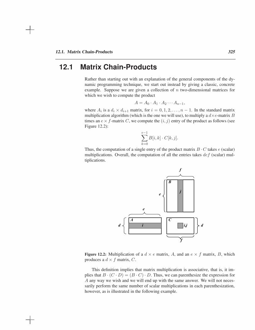
multiplication algorithm (which is the one we will use), to multiply a d×e-matrix Btimes an e× f -matrix C , we compute the (i, j) entry of the product as follows (see
Figure 12.2):
e−1∑
k=0
B[i, k] · C[k, j].
Thus, the computation of a single entry of the product matrix B ·C takes e (scalar)
multiplications. Overall, the computation of all the entries takes def (scalar) mul-
tiplications.
A C
B
d d
f
e
f
e
i
j
i,j
Figure 12.2: Multiplication of a d × e matrix, A, and an e × f matrix, B, which
produces a d× f matrix, C .
This definition implies that matrix multiplication is associative, that is, it im-
plies that B · (C ·D) = (B · C) ·D. Thus, we can parenthesize the expression for
A any way we wish and we will end up with the same answer. We will not neces-
sarily perform the same number of scalar multiplications in each parenthesization,
however, as is illustrated in the following example.

326 Chapter 12. Dynamic Programming
Example 12.1: Let B be a 2×10-matrix, let C be a 10×50-matrix, and let D bea 50× 20-matrix. Computing B · (C ·D) requires 2 · 10 · 20+10 · 50 · 20 = 10400multiplications, whereas computing (B ·C)·D requires 2·10·50+2·50·20 = 3000multiplications.
The matrix chain-product problem is to determine the parenthesization of the
expression defining the product A that minimizes the total number of scalar multi-
plications performed. Of course, one way to solve this problem is to simply enu-
merate all the possible ways of parenthesizing the expression for A and determine
the number of multiplications performed by each one. Unfortunately, the set of all
different parenthesizations of the expression for A is equal in number to the set of
all different binary trees that have n external nodes. This number is exponential in
n. Thus, this straightforward (“brute force”) algorithm runs in exponential time, for
there are an exponential number of ways to parenthesize an associative arithmetic
expression (the number is equal to the nth Catalan number, which is Ω(4n/n3/2)).
Defining Subproblems
We can improve the performance achieved by the brute force algorithm signifi-
cantly, however, by making a few observations about the nature of the matrix chain-
product problem. The first observation is that the problem can be split into subprob-
lems. In this case, we can define a number of different subproblems, each of which
is to compute the best parenthesization for some subexpression Ai · Ai+1 · · ·Aj .
As a concise notation, we use Ni,j to denote the minimum number of multipli-
cations needed to compute this subexpression. Thus, the original matrix chain-
product problem can be characterized as that of computing the value of N0,n−1.
This observation is important, but we need one more in order to apply the dynamic
programming technique.
Characterizing Optimal Solutions
The other important observation we can make about the matrix chain-product prob-
lem is that it is possible to characterize an optimal solution to a particular subprob-
lem in terms of optimal solutions to its subproblems. We call this property the
subproblem optimality condition.
In the case of the matrix chain-product problem, we observe that, no mat-
ter how we parenthesize a subexpression, there has to be some final matrix mul-
tiplication that we perform. That is, a full parenthesization of a subexpression
Ai · Ai+1 · · ·Aj has to be of the form (Ai · · ·Ak) · (Ak+1 · · ·Aj), for some k ∈i, i + 1, . . . , j − 1. Moreover, for whichever k is the right one, the products
(Ai · · ·Ak) and (Ak+1 · · ·Aj) must also be solved optimally. If this were not so,
then there would be a global optimal that had one of these subproblems solved
suboptimally. But this is impossible, since we could then reduce the total number

12.1. Matrix Chain-Products 327
of multiplications by replacing the current subproblem solution by an optimal so-
lution for the subproblem. This observation implies a way of explicitly defining
the optimization problem for Ni,j in terms of other optimal subproblem solutions.
Namely, we can compute Ni,j by considering each place k where we could put the
final multiplication and taking the minimum over all such choices.
Designing a Dynamic Programming Algorithm
The above discussion implies that we can characterize the optimal subproblem so-
lution Ni,j as
Ni,j = mini≤k<j
Ni,k +Nk+1,j + didk+1dj+1,
where we note that Ni,i = 0, since no work is needed for a subexpression compris-
ing a single matrix. That is, Ni,j is the minimum, taken over all possible places to
perform the final multiplication, of the number of multiplications needed to com-
pute each subexpression plus the number of multiplications needed to perform the
final matrix multiplication.
The equation for Ni,j looks similar to the recurrence equations we derive for
divide-and-conquer algorithms, but this is only a superficial resemblance, for there
is an aspect of the equation for Ni,j that makes it difficult to use divide-and-conquer
to compute Ni,j . In particular, there is a sharing of subproblems going on that
prevents us from dividing the problem into completely independent subproblems
(as we would need to do to apply the divide-and-conquer technique). We can,
nevertheless, use the equation for Ni,j to derive an efficient algorithm by computing
Ni,j values in a bottom-up fashion, and storing intermediate values in a table of Ni,j
values. We can begin simply enough by assigning Ni,i = 0 for i = 0, 1, . . . , n− 1.
We can then apply the general equation for Ni,j to compute Ni,i+1 values, since
they depend only on Ni,i and Ni+1,i+1 values, which are available. Given the
Ni,i+1 values, we can then compute the Ni,i+2 values, and so on. Therefore, we can
build Ni,j values up from previously computed values until we can finally compute
the value of N0,n−1, which is the number that we are searching for. The details of
this dynamic programming solution are given in Algorithm 12.3.
Analyzing the Matrix Chain-Product Algorithm
Thus, we can compute N0,n−1 with an algorithm that consists primarily of three
nested for-loops. The outside loop is executed n times. The loop inside is exe-
cuted at most n times. And the inner-most loop is also executed at most n times.
Therefore, the total running time of this algorithm is O(n3).
Theorem 12.2: Given a chain-product of n two-dimensional matrices, we cancompute a parenthesization of this chain that achieves the minimum number of
scalar multiplications in O(n3) time.

328 Chapter 12. Dynamic Programming
Algorithm MatrixChain(d0, . . . , dn):
Input: Sequence d0, . . . , dn of integers
Output: For i, j = 0, . . . , n − 1, the minimum number of multiplications Ni,j
needed to compute the product Ai · Ai+1 · · ·Aj , where Ak is a dk × dk+1
matrix
for i← 0 to n− 1 do
Ni,i ← 0for b← 1 to n− 1 do
for i← 0 to n− b− 1 do
j ← i+ bNi,j ← +∞for k ← i to j − 1 do
Ni,j ← minNi,j, Ni,k +Nk+1,j + didk+1dj+1.
Algorithm 12.3: Dynamic programming algorithm for the matrix chain-product
problem.
Proof: We have shown above how we can compute the optimal number of scalar
multiplications. But how do we recover the actual parenthesization?
The method for computing the parenthesization itself is is actually quite straight-
forward. We modify the algorithm for computing Ni,j values so that any time we
find a new minimum value for Ni,j , we store, with Ni,j , the index k that allowed
us to achieve this minimum.
In Figure 12.4, we illustrate the way the dynamic programming solution to the
matrix chain-product problem fills in the array N .
i
j
i,k
k+1,j
i,j
+ didk+1dj+1
N
Figure 12.4: Illustration of the way the matrix chain-product dynamic-programming
algorithm fills in the array N .
Now that we have worked through a complete example of the use of the dy-
namic programming method, we discus in the next section the general aspects of
the dynamic programming technique as it can be applied to other problems.

12.2. The General Technique 329
12.2 The General Technique
The dynamic programming technique is used primarily for optimization problems,
where we wish to find the “best” way of doing something. Often the number of
different ways of doing that “something” is exponential, so a brute-force search
for the best is computationally infeasible for all but the smallest problem sizes.
We can apply the dynamic programming technique in such situations, however, if
the problem has a certain amount of structure that we can exploit. This structure
involves the following three components:
Simple Subproblems: There has to be some way of breaking the global optimiza-
tion problem into subproblems, each having a similar structure to the original
problem. Moreover, there should be a simple way of defining subproblems
with just a few indices, like i, j, k, and so on.
Subproblem Optimality: An optimal solution to the global problem must be a
composition of optimal subproblem solutions, using a relatively simple com-
bining operation. We should not be able to find a globally optimal solution
that contains suboptimal subproblems.
Subproblem Overlap: Optimal solutions to unrelated subproblems can contain
subproblems in common. Indeed, such overlap allows us to improve the
efficiency of a dynamic programming algorithm by storing solutions to sub-
problems.
This last property is particularly important for dynamic programming algo-
rithms, because it allows them to take advantage of memoization, which is an
optimization that allows us to avoid repeated recursive calls by storing interme-
diate values. Typically, these intermediate values are indexed by a small set of
parameters, and we can store them in an array and look them up as needed.
As an illustration of the power of memoization, consider the Fibonacci series,
f(n), defined as
f(0) = 0
f(1) = 1
f(n) = f(n− 1) + f(n− 2).
If we implement this equation literally, as a recursive program, then the running
time of our algorithm, T (n), as a function of n, has the following behavior:
T (0) = 1
T (1) = 1
T (n) = T (n− 1) + T (n− 2).
But this implies that
T (n) ≥ 2T (n− 2) = 2n/2.

330 Chapter 12. Dynamic Programming
In other words, if we implement this equation recursively as written, then our run-
ning time is exponential in n. But if we store Fibonacci numbers in an array, F ,
then we can instead calculate the Fibonacci number, F [n], iteratively, as follows:
F [0]← 0F [1]← 1for i = 2 to n do
F [i]← F [i− 1] + F [i− 2]
This algorithm clearly runs in O(n) time, and it illustrates the way memoization
can lead to improved performance when subproblems overlap and we use table
lookups to avoid repeating recursive calls. (See Figure 12.5.)
!"#$%
!"&$%!"'$%
!"($%!"&$%!"'$%
!"($%
!"&$%
!")$%
!"*$%
!"&$%!"'$%
!"($%!"&$%
!")$%
(a)
!"#$%!"&$%
!"'$%!"($%
!")$%!"*$%
(b)
Figure 12.5: The power of memoization. (a) all the function calls needed for a
fully recursive definition of the Fibonacci function; (b) the data dependencies in an
iterative definition.

12.3. Telescope Scheduling 331
12.3 Telescope Scheduling
Large, powerful telescopes are precious resources that are typically oversubscribed
by the astronomers who request times to use them. This high demand for observa-
tion times is especially true, for instance, for the Hubble Space Telescope, which
receives thousands of observation requests per month. In this section, we consider a
simplified version of the problem of scheduling observations on a telescope, which
factors out some details, such as the orientation of the telescope for an observation
and who is requesting that observation, but which nevertheless keeps some of the
more important aspects of this problem.
The input to this telescope scheduling problem is a list, L, of observation re-
quests, where each request, i, consists of the following elements:
• a requested start time, si, which is the moment when a requested observation
should begin
• a finish time, fi, which is the moment when the observation should finish
(assuming it begins at its start time)
• a positive numerical benefit, bi, which is an indicator of the scientific gain to
be had by performing this observation.
The start and finish times for a observation request are specified by the astronomer
requesting the observation; the benefit of a request is determined by an administra-
tor or a review committee for the telescope. To get the benefit, bi, for an observation
request, i, that observation must be performed by the telescope for the entire time
period from the start time, si, to the finish time, fi. Thus, two requests, i and j,
conflict if the time interval [si, fi], intersects the time interval, [sj , fj]. Given the
list, L, of observation requests, the optimization problem is to schedule observa-
tion requests in a non-conflicting way so as to maximize the total benefit of the
observations that are included in the schedule.
There is an obvious exponential-time algorithm for solving this problem, of
course, which is to consider all possible subsets of L and choose the one that has
the highest total benefit without causing any scheduling conflicts. We can do much
better than this, however, by using the dynamic programming technique.
As a first step towards a solution, we need to define subproblems. A natural way
to do this is to consider the observation requests according to some ordering, such
as ordered by start times, finish times, or benefits. Start times and finish times are
essentially symmetric, so we can immediately reduce the choice to that of picking
between ordering by finish times and ordering by benefits.
The greedy strategy would be to consider the observation requests ordered by
non-increasing benefits, and include each request that doesn’t conflict with any cho-
sen before it. This strategy doesn’t lead to an optimal solution, however, which we
can see after considering a simple example. For instance, suppose we had a list con-
taining just 3 requests—one with benefit 100 that conflicts with two non-conflicting

332 Chapter 12. Dynamic Programming
!"
#"
$"
%"
&"
'"
("
)*+,*+-."
&"
$"
&"
%"
#"
&"
$"
)*/0/1/22,*"
3"
3"
!"
3"
$"
&"
#"
4,567,89"!" $"
&"'"
Figure 12.6: The telescope scheduling problem. The left and right boundary of each
rectangle represent the start and finish times for an observation request. The height
of each rectangle represents its benefit. We list each request’s benefit on the left
and its predecessor on the right. The requests are listed by increasing finish times.
The optimal solution has total benefit 17.
requests with benefit 75 each. The greedy algorithm would choose the observation
with benefit 100, in this case, whereas we could achieve a total benefit of 150 by
taking the two requests with benefit 75 each. So a greedy strategy based on repeat-
edly choosing a non-conflicting request with maximum benefit won’t work.
Let us assume, therefore, that the observation requests in L are sorted by non-
decreasing finish times, as shown in Figure 12.6. The idea in this case would be
to consider each request according to this ordering. So let us define our set of
subproblems in terms of a parameter, Bi, which is defined as follows:
Bi = the maximum benefit that can be achieved with the first i requests in L.
So, as a boundary condition, we get that B0 = 0.
One nice observation that we can make for this ordering of L by non-decreasing
finish times is that, for any request i, the set of other requests that conflict with iform a contiguous interval of requests in L. Define the predecessor, pred(i), for
each request, i, then, to be the largest index, j < i, such that request i and j don’t
conflict. If there is no such index, then define the predecessor of i to be 0. (See
Figure 12.6.)
The definition of the predecessor of each request lets us easily reason about the
effect that including or not including an observation request, i, in a schedule that
includes the first i requests in L. That is, in a schedule that achieves the optimal

12.3. Telescope Scheduling 333
value, Bi, for i ≥ 1, either it includes the observation i or it doesn’t; hence, we can
reason as follows:
• If the optimal schedule achieving the benefit Bi includes observation i, then
Bi = Bpred(i) + bi. If this were not the case, then we could get a better
benefit by substituting the schedule achieving Bpred(i) for the one we used
from among those with indices at most pred(i).• On the other hand, if the optimal schedule achieving the benefit Bi does not
include observation i, then Bi = Bi−1. If this were not the case, then we
could get a better benefit by using the schedule that achieves Bi−1.
Therefore, we can make the following recursive definition:
Bi = maxBi−1, Bpred(i) + bi.Notice that this definition exhibits subproblem overlap. Thus, it is most efficient
for us to use memoization when computing Bi values, by storing them in an array,
B, which is indexed from 0 to n. Given the ordering of requests by finish times
and an array, P , so that P [i] = pred(i), then we can fill in the array, B, using the
following simple algorithm:
B[0]← 0for i = 1 to n do
B[i]← maxB[i− 1], B[P [i]] + bi
After this algorithm completes, the benefit of the optimal solution will be B[n],and, to recover an optimal schedule, we simply need to trace backwards in B from
this point. During this trace, if B[i] = B[i − 1], then we can assume observa-
tion i is not included and move next to consider observation i − 1. Otherwise, if
B[i] = B[P [i]] + bi, then we can assume observation i is included and move next
to consider observation P [i].It is easy to see that the running time of this algorithm is O(n), but it assumes
that we are given the list L ordered by finish times and that we are also given the
predecessor index for each request i. Of course, we can easily sort L by finish times
if it is not given to us already sorted according to this ordering. To compute the
predecessor of each request, note that it is sufficient that we also have the requests
in L sorted by start times. In particular, given a listing of L ordered by finish times
and another listing, L′, ordered by start times, then a merging of these two lists, as
in the merge-sort algorithm (Section 8.1), gives us what we want. The predecessor
of request i is literally the index of the predecessor in L of the value, si, in L′.
Therefore, we have the following.
Theorem 12.3: Given a list, L, of n observation requests, provided in two sortedorders, one by non-decreasing finish times and one by non-decreasing start times,
we can solve the telescope scheduling problem for L in O(n) time.

334 Chapter 12. Dynamic Programming
12.4 Game Strategies
There are many types of games, some that are completely random and others where
players benefit by employing various kinds of strategies. In this section, we con-
sider two simple games in which dynamic programming can be employed to come
up with optimal strategies for playing these games. These are not the only game
scenarios where dynamic programming applies, however, as it has been used to ana-
lyze strategies for many other games as well, including baseball, American football,
and cricket.
12.4.1 Coins in a Line
The first game we consider is reported to arise in a problem that is sometimes asked
during job interviews at major software and Internet companies (probably because
it is so tempting to apply a greedy strategy to this game, whereas the optimal strat-
egy uses dynamic programming).
In this game, which we will call the coins-in-a-line game, an even number, n,
of coins, of various denominations from various countries, are placed in a line. Two
players, who we will call Alice and Bob, take turns removing one of the coins from
either end of the remaining line of coins. That is, when it is a player’s turn, he or
she removes the coin at the left or right end of the line of coins and adds that coin to
his or her collection. The player who removes a set of coins with larger total value
than the other player wins, where we assume that both Alice and Bob know the
value of each coin in some common currency, such as dollars. (See Figure 12.7.)
!"# !$# !%# !&# !'# !$#
()*+,-#./0#!"10#."0#!$10#.20#!&1########3456)#76)8,#9#!/:###
;4<-#.%0#!$10#.$0#!'10#.'0#!%1########3456)#76)8,#9#!/=###
/# %# '# 2# $# "#
Figure 12.7: The coins-in-a-line game. In this instance, Alice goes first and ul-
timately ends up with $18 worth of coins. U.S. government images. Credit:
U.S. Mint.

12.4. Game Strategies 335
A Dynamic Programming Solution
It is tempting to start thinking of various greedy strategies, such as always choosing
the largest-valued coin, minimizing the two remaining choices for the opponent, or
even deciding in advance whether it is better to choose all the odd-numbered coins
or even-numbered coins. Unfortunately, none of these strategies will consistently
lead to an optimal strategy for Alice to play the coins-in-a-line game, assuming that
Bob follows an optimal strategy for him.
To design an optimal strategy, we apply the dynamic programming technique.
In this case, since Alice and Bob can remove coins from either end of the line,
the appropriate way to define subproblems is in terms of a range of indices for the
coins, assuming they are initially numbered from 1 to n, as in Figure 12.7. Thus,
let us define the following indexed parameter:
Mi,j =
the maximum value of coins taken by Alice, for coins
numbered i to j, assuming Bob plays optimally.
Therefore, the optimal value for Alice is determined by M1,n.
Let us assume that the values of the coins are stored in an array, V , so that coin
1 is of Value V [1], coin 2 is of Value V [2], and so on. To determine a recursive
definition for Mi,j , we note that, given the line of coins from coin i to coin j, the
choice for Alice at this point is either to take coin i or coin j and thereby gain
a coin of value V [i] or V [j]. Once that choice is made, play turns to Bob, who
we are assuming is playing optimally. Thus, he will make the choice among his
possibilities that minimizes the total amount that Alice can get from the coins that
remain. In other words, Alice must choose based on the following reasoning:
• If j = i+ 1, then she should pick the larger of V [i] and V [j], and the game
is over.
• Otherwise, if Alice chooses coin i, then she gets a total value of
minMi+1,j−1, Mi+2,j+ V [i].
• Otherwise, if Alice chooses coin j, then she gets a total value of
minMi,j−2, Mi+1,j−1+ V [j].
Since these are all the choices that Alice has, and she is trying to maximize her
returns, then we get the following recurrence equation, for j > i+1, where j−i+1is even:
Mi,j = max minMi+1,j−1, Mi+2,j+ V [i], minMi,j−2, Mi+1,j−1+ V [j] .
In addition, for i = 1, 2, . . . , n− 1, we have the initial conditions

336 Chapter 12. Dynamic Programming
Mi,i+1 = maxV [i], V [i+ 1].
We can compute the Mi,j values, then, using memoization, by starting with the
definitions for the above initial conditions and then computing all the Mi,j’s where
j − i + 1 is 4, then for all such values where j − i + 1 is 6, and so on. Since
there are O(n) iterations in this algorithm and each iteration runs in O(n) time, the
total time for this algorithm is O(n2). Of course, this algorithm simply computes
all the relevant Mi,j values, including the final value, M1,n. To recover the actual
game strategy for Alice (and Bob), we simply need to note for each Mi,j whether
Alice should choose coin i or coin j, which we can determine from the definition
of Mi,j . And given this choice, we then know the optimal choice for Bob, and that
determines if the next choice for Alice is based on Mi+2,j , Mi+1,j−1, or Mi,j−2.
Therefore, we have the following.
Theorem 12.4: Given an even number, n, of coins in a line, all of known values,
we can determine in O(n2) time the optimal strategy for the first player, Alice, tomaximize her returns in the coins-in-a-line game, assuming Bob plays optimally.
12.4.2 Probabilistic Game Strategies and Backward Induction
In addition to games, like chess and the coins-in-a-line game, which are purely
strategic, there are lots of games that involve some combination of strategy and
randomness (or events that can be modeled probabilistically), like backgammon
and sports. Another application of dynamic programming in the context of games
arises in these games, in a way that involves combining probability and optimiza-
tion. To illustrate this point, we consider in this section a strategic decision that
arises in the game of American football, which hereafter we refer to simply as
“football.”
Extra Points in Football
After a team scores a touchdown in football, they have have a choice between
kicking an extra point, which involves kicking the ball through the goal posts to
add 1 point to their score if this is successful, or attempting a two-point conversion,
which involves lining up again and advancing the ball into the end zone to add 2
points to their score if this is successful. In professional football teams, extra point
attempts are successful with a probability of .98 and two-point conversion have a
success probability between .40 and .55, depending on the team.
In addition to these probabilistic considerations, the choice of whether it is
better to attempt a two-point conversion or not also depends on the difference in
the scores between the two teams and how many possessions are left in the game
(a possession is a sequence of plays where one team has control of the ball).

12.4. Game Strategies 337
Developing a Recurrence Equation
Let us characterize the state of a football game in terms of a triple, (k, d, n), where
these parameters have the following meanings:
• k is the number of points scored at the end of a possession (0 for no score,
3 for a field goal, and 6 for a touchdown, as we are ignoring safeties and
we are counting the effects of extra points after a touchdown separately).
Possessions alternate between team A and team B.
• d is the difference in points between team A and team B (which is positive
when A is in the lead and negative when B is in the lead).
• n is the number of possessions remaining in the game.
For the sake of this analysis, let us assume that n is a potentially unbounded param-
eter that is known to the two teams, whereas k is always a constant and d can be
considered a constant as well, since no professional football team has come back
from a point deficit of −30 to win.
We can then define VA(k, d, n) to be the probability that team A wins the
game given that its possession ended with team A scoring k points to now have
a score deficit of d and n more possessions remaining in the game. Similarly, de-
fine VB(k, d, n) to be the probability that team A wins the game given that team
B’s possession ended with team B scoring k points to now cause team A to have a
score deficit of d with n more possessions remaining in the game. Thus, team A is
trying to maximize VA and team B is trying to minimize VB .
To derive recursive definitions for VA and VB , note that at the end of the game,
when n = 0, the outcome is determined. Thus, VA(k, d, 0) = 1 if and only if
d > 0, and similarly for VB(k, d, 0). We assume, based on past performance, that
we know the probability that team A or B will score a touchdown or field goal in
a possession, and that these probabilities are independent of k, d, or n. Thus, we
can determine V (k, d, n), the probability that A wins after completing a possession
with no score (k = 0) or a field goal (k = 3) as follows:
VA(0, d, n) = VA(3, d, n) = Pr(TD by B)VB(6, d− 6, n − 1)
+Pr(FG by B)VB(3, d− 3, n − 1)
+Pr(NS by B)VB(0, d, n − 1).
The first term quantifies the impact of team B scoring a touchdown (TD) on the
next possession, the second term quantifies the impact of team B scoring a field
goal (FG) on the next possession, and the third term quantifies the impact of team
B having no score (NS) at the end of the next possession. Similar equations hold for
VB, with the roles of A and B reversed. For professional football teams, the average
probability of a possession ending in a touchdown is .20, the average probability
of a possession ending in a field goal is .12; hence, for such an average team, we
would take the probability of a possession ending with no score for team B to be
.68. The main point of this exercise, however, is to characterize the case when
k = 6, that is, when a possession ends with a touchdown.

338 Chapter 12. Dynamic Programming
Let p1 denote the probability of success for a extra-point attempt and p2 denote
the probability of success for a two-point conversion. Then we have
1. Pr(Team A wins if it makes an extra point attempt in state (6, d, n))
= p1 [Pr(TD by B)VB(6, d − 5, n − 1)
+Pr(FG by B)VB(3, d− 2, n − 1)
+ Pr(NS by B)VB(0, d+ 1, n − 1)]
+ (1− p1) [Pr(TD by B)VB(6, d − 6, n − 1)
+Pr(FG by B)VB(3, d − 3, n− 1)
+ Pr(NS by B)VB(0, d, n − 1)] .
2. Pr(Team A wins if it tries a two-point conversion in state (6, d, n))
= p2 [Pr(TD by B)VB(6, d − 4, n − 1)
+Pr(FG by B)VB(3, d − 1, n− 1)
+ Pr(NS by B)VB(0, d + 2, n − 1)]
+ (1− p2) [Pr(TD by B)VB(6, d − 6, n − 1)
+Pr(FG by B)VB(3, d − 3, n − 1)
+ Pr(NS by B)VB(0, d, n − 1)] .
The value of VA(6, d, n) is the maximum of the above two probabilities. Similar
bounds hold for VB , except that VB(6, d, n) is the minimum of the two similarly-
defined probabilities. Given our assumptions about k and d, these equations imply
that we can compute V (k, d, n) in O(n) time, by incrementally increasing the value
of n in the above equations and applying memoization. Note that this amounts to
reasoning about the game backwards, in that we start with an ending state and use
a recurrence equation to reason backward in time. For this reason, this analysis
technique is called backward induction.
In the case of the decision we are considering, given known statistics for an
average professional football team, the values of n for when it is better to attempt
a two-point conversion are shown in Table 12.8.
behind by (−d) 1 2 3 4 5 6 7 8 9 10
n range ∅ [0, 15] ∅ ∅ [2, 14] ∅ ∅ [2, 8] [4, 9] [2, 5]
ahead by (d) 0 1 2 3 4 5 6 7 8 9 10
n range ∅ [1, 7] [4, 10] ∅ ∅ [1, 15] ∅ ∅ ∅ ∅ ∅
Table 12.8: When it is preferential to attempt a two-point conversion after a touch-
down, based on n, the number of possessions remaining in a game. Each interval
indicates the range of values of n for which it is better to make such an attempt.

12.5. The Longest Common Subsequence Problem 339
12.5 The Longest Common Subsequence Problem
A common text processing problem, which, we mentioned in the introduction,
arises in genetics, is to test the similarity between two text strings. Recall that,
in the genetics application, the two strings correspond to two strands of DNA,
which could, for example, come from two individuals, who we will consider ge-
netically related if they have a long subsequence common to their respective DNA
sequences. There are other applications, as well, such as in software engineering,
where the two strings could come from two versions of source code for the same
program, and we may wish to determine which changes were made from one ver-
sion to the next. In addition, the data gathering systems of search engines, which
are called Web crawlers, must be able to distinguish between similar Web pages
to avoid needless Web page requests. Indeed, determining the similarity between
two strings is considered such a common operation that the Unix/Linux operating
systems come with a program, called diff, for comparing text files.
12.5.1 Problem Definition
There are several different ways we can define the similarity between two strings.
Even so, we can abstract a simple, yet common, version of this problem using
character strings and their subsequences. Given a string X of size n, a subsequence
of X is any string that is of the form
X[i1]X[i2] · · ·X[ik], ij < ij+1 for j = 1, . . . , k;
that is, it is a sequence of characters that are not necessarily contiguous but are nev-
ertheless taken in order from X. For example, the string AAAG is a subsequence
of the string CGATAATTGAGA. Note that the concept of subsequence of a
string is different from the one of substring of a string.
The specific text similarity problem we address here is the longest common
subsequence (LCS) problem. In this problem, we are given two character strings,
X of size n and Y of size m, over some alphabet and are asked to find a longest
string S that is a subsequence of both X and Y .
One way to solve the longest common subsequence problem is to enumerate
all subsequences of X and take the largest one that is also a subsequence of Y .
Since each character of X is either in or not in a subsequence, there are potentially
2n different subsequences of X, each of which requires O(m) time to determine
whether it is a subsequence of Y . Thus, the brute-force approach yields an ex-
ponential algorithm that runs in O(2nm) time, which is very inefficient. In this
section, we discuss how to use dynamic programming to solve the longest com-
mon subsequence problem much faster than this.

340 Chapter 12. Dynamic Programming
12.5.2 Applying Dynamic Programming to the LCS Problem
We can solve the LCS problem much faster than exponential time using dynamic
programming. As mentioned above, one of the key components of the dynamic
programming technique is the definition of simple subproblems that satisfy the
subproblem optimization and subproblem overlap properties.
Recall that in the LCS problem, we are given two character strings, X and Y ,
of length n and m, respectively, and are asked to find a longest string S that is a
subsequence of both X and Y . Since X and Y are character strings, we have a
natural set of indices with which to define subproblems—indices into the strings Xand Y . Let us define a subproblem, therefore, as that of computing the length of
the longest common subsequence of X[0..i] and Y [0..j], denoted L[i, j].
This definition allows us to rewrite L[i, j] in terms of optimal subproblem so-
lutions. We consider the following two cases. (See Figure 12.9.)
Case 1: X[i] = Y [j]. Let c = X[i] = Y [j]. We claim that a longest common
subsequence of X[0..i] and Y [0..j] ends with c. To prove this claim, let us
suppose it is not true. There has to be some longest common subsequence
X[i1]X[i2] . . . X[ik] = Y [j1]Y [j2] . . . Y [jk]. If X[ik] = c or Y [jk] = c,then we get the same sequence by setting ik = i and jk = j. Alternately, if
X[jk] 6= c, then we can get an even longer common subsequence by adding
c to the end. Thus, a longest common subsequence of X[0..i] and Y [0..j]ends with c = X[i] = Y [j]. Therefore, we set
L[i, j] = L[i− 1, j − 1] + 1 if X[i] = Y [j]. (12.1)
Case 2: X[i] 6= Y [j]. In this case, we cannot have a common subsequence that
includes both X[i] and Y [j]. That is, a common subsequence can end with
X[i], Y [j], or neither, but not both. Therefore, we set
L[i, j] = maxL[i− 1, j] , L[i, j − 1] if X[i] 6= Y [j]. (12.2)
In order to make Equations 12.1 and 12.2 make sense in the boundary cases when
i = 0 or j = 0, we define L[i,−1] = 0 for i = −1, 0, 1, . . . , n−1 and L[−1, j] = 0for j = −1, 0, 1, . . . ,m− 1.
Y=CGA T AA TTGA G
X=GTTCCT AA T A
Y=CGA T AA TTGA G A
X=GTTCCT AA T A
(a) (b)
0 1 2 3 4 5 6 7 8 90 1 2 3 4 5 6 7 8 9
0 1 2 3 4 5 6 7 8 9 10 11 0 1 2 3 4 5 6 7 8 9 10
L [8,10]=5L [8,10]=5
L [9,9]=6
Figure 12.9: The two cases for L[i, j]: (a) X[i] = Y [j]; (b) X[i] 6= Y [j].
12.5. The Longest Common Subsequence Problem 341
The LCS Algorithm
The above definition of L[i, j] satisfies subproblem optimization, for we cannot
have a longest common subsequence without also having longest common subse-
quences for the subproblems. Also, it uses subproblem overlap, because a subprob-
lem solution L[i, j] can be used in several other problems (namely, the problems
L[i+ 1, j], L[i, j + 1], and L[i+ 1, j + 1]).
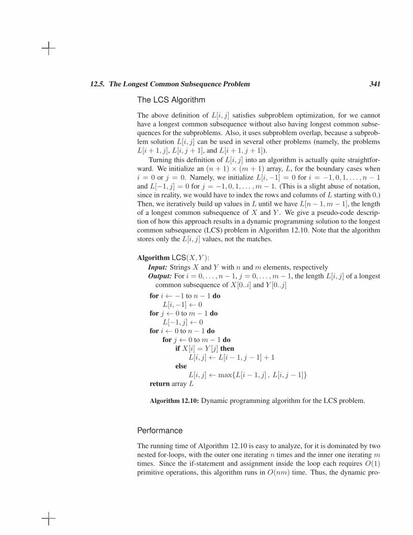
Turning this definition of L[i, j] into an algorithm is actually quite straightfor-
ward. We initialize an (n + 1) × (m + 1) array, L, for the boundary cases when
i = 0 or j = 0. Namely, we initialize L[i,−1] = 0 for i = −1, 0, 1, . . . , n − 1and L[−1, j] = 0 for j = −1, 0, 1, . . . ,m − 1. (This is a slight abuse of notation,
since in reality, we would have to index the rows and columns of L starting with 0.)
Then, we iteratively build up values in L until we have L[n− 1,m− 1], the length
of a longest common subsequence of X and Y . We give a pseudo-code descrip-
tion of how this approach results in a dynamic programming solution to the longest
common subsequence (LCS) problem in Algorithm 12.10. Note that the algorithm
stores only the L[i, j] values, not the matches.
Algorithm LCS(X,Y ):
Input: Strings X and Y with n and m elements, respectively
Output: For i = 0, . . . , n− 1, j = 0, . . . ,m− 1, the length L[i, j] of a longest
common subsequence of X[0..i] and Y [0..j]
for i← −1 to n− 1 do
L[i,−1]← 0for j ← 0 to m− 1 do
L[−1, j]← 0for i← 0 to n− 1 do
for j ← 0 to m− 1 do
if X[i] = Y [j] then
L[i, j]← L[i− 1, j − 1] + 1else
L[i, j]← maxL[i− 1, j] , L[i, j − 1]return array L
Algorithm 12.10: Dynamic programming algorithm for the LCS problem.
Performance
The running time of Algorithm 12.10 is easy to analyze, for it is dominated by two
nested for-loops, with the outer one iterating n times and the inner one iterating mtimes. Since the if-statement and assignment inside the loop each requires O(1)primitive operations, this algorithm runs in O(nm) time. Thus, the dynamic pro-

342 Chapter 12. Dynamic Programming
gramming technique can be applied to the longest common subsequence problem
to improve significantly over the exponential-time brute-force solution to the LCS
problem.
Algorithm LCS (12.10) computes the length of the longest common subse-
quence (stored in L[n− 1,m− 1]), but not the subsequence itself. As shown in the
following theorem, a simple postprocessing step can extract the longest common
subsequence from the array L returned by the algorithm.
Theorem 12.5: Given a string X of n characters and a string Y of m characters,we can find the longest common subsequence of X and Y in O(nm) time.
Proof: We have already observed that Algorithm LCS computes the length
of a longest common subsequence of the input strings X and Y in O(nm) time.
Given the table of L[i, j] values, constructing a longest common subsequence is
straightforward. One method is to start from L[n−1,m−1] and work back through
the table, reconstructing a longest common subsequence from back to front. At
any position L[i, j], we determine whether X[i] = Y [j]. If this is true, then we
take X[i] as the next character of the subsequence (noting that X[i] is before the
previous character we found, if any), moving next to L[i−1, j−1]. If X[i] 6= Y [j],then we move to the larger of L[i, j − 1] and L[i − 1, j]. (See Figure 12.11.) We
stop when we reach a boundary entry (with i = −1 or j = −1). This method
constructs a longest common subsequence in O(n+m) additional time.
Y=CGATAATTGAGA
X=GTTCCTAATA
L -1 0 1 2 3 4 5 6 7 8 9 10 11
-1 0 0 0 0 0 0 0 0 0 0 0 0 0
0 0 0 1 1 1 1 1 1 1 1 1 1 1
1 0 0 1 1 2 2 2 2 2 2 2 2 2
2 0 0 1 1 2 2 2 3 3 3 3 3 3
3 0 1 1 1 2 2 2 3 3 3 3 3 3
4 0 1 1 1 2 2 2 3 3 3 3 3 3
5 0 1 1 1 2 2 2 3 4 4 4 4 4
6 0 1 1 2 2 3 3 3 4 4 5 5 5
7 0 1 1 2 2 3 4 4 4 4 5 5 6
8 0 1 1 2 3 3 4 5 5 5 5 5 6
9 0 1 1 2 3 4 4 5 5 5 6 6 6
0 1 2 3 4 5 6 7 8 91011
0 1 2 3 4 5 6 7 8 9
Figure 12.11: Illustration of the algorithm for constructing a longest common sub-
sequence from the array L.

12.6. The 0-1 Knapsack Problem 343
12.6 The 0-1 Knapsack Problem
Suppose a hiker is about to go on a trek through a rain forest carrying a single
knapsack. Suppose further that she knows the maximum total weight W that she
can carry, and she has a set S of n different useful items that she can potentially
take with her, such as a folding chair, a tent, and a copy of this book. Let us assume
that each item i has an integer weight wi and a benefit value bi, which is the utility
value that our hiker assigns to item i. Her problem, of course, is to optimize the
total value of the set T of items that she takes with her, without going over the
weight limit W . That is, she has the following objective:
maximize∑
i∈T
bi subject to∑
i∈T
wi ≤W.
Her problem is an instance of the 0-1 knapsack problem. This problem is called
a “0-1” problem, because each item must be entirely accepted or rejected. We
consider the fractional version of this problem in Section 10.1, and we study how
knapsack problems arise in the context of Internet auctions in Exercise R-12.9.
A Pseudo-Polynomial Time Dynamic Programming Algorithm
We can easily solve the 0-1 knapsack problem in Θ(2n) time, of course, by enu-
merating all subsets of S and selecting the one that has highest total benefit from
among all those with total weight not exceeding W . This would be an inefficient
algorithm, however. Fortunately, we can derive a dynamic programming algorithm
for the 0-1 knapsack problem that runs much faster than this in most cases.
As with many dynamic programming problems, one of the hardest parts of
designing such an algorithm for the 0-1 knapsack problem is to find a nice char-
acterization for subproblems (so that we satisfy the three properties of a dynamic
programming algorithm). To simplify the discussion, number the items in S as
1, 2, . . . , n and define, for each k ∈ 1, 2, . . . , n, the subset
Sk = items in S labeled 1, 2, . . . , k.One possibility is for us to define subproblems by using a parameter k so that
subproblem k is the best way to fill the knapsack using only items from the set Sk.
This is a valid subproblem definition, but it is not at all clear how to define an
optimal solution for index k in terms of optimal subproblem solutions. Our hope
would be that we would be able to derive an equation that takes the best solution
using items from Sk−1 and considers how to add the item k to that. Unfortunately,
if we stick with this definition for subproblems, then this approach is fatally flawed.
For, as we show in Figure 12.12, if we use this characterization for subproblems,
then an optimal solution to the global problem may actually contain a suboptimal
subproblem.

344 Chapter 12. Dynamic Programming
(3,2) (5,4) (8,5) (10,9)
(8,5)(5,4) (4,3)(a)
(b)
(3,2)
20
Figure 12.12: An example showing that our first approach to defining a knapsack
subproblem does not work. The set S consists of five items denoted by the the
(weight, benefit) pairs (3, 2), (5, 4), (8, 5), (4, 3), and (10, 9). The maximum total
weight is W = 20: (a) best solution with the first four items; (b) best solution with
the first five items. We shade each item in proportion to its benefit.
One of the reasons that defining subproblems only in terms of an index k is
fatally flawed is that there is not enough information represented in a subproblem
to provide much help for solving the global optimization problem. We can correct
this difficulty, however, by adding a second parameter w. Let us therefore formulate
each subproblem as that of computing B[k,w], which is defined as the maximum
total value of a subset of Sk from among all those subsets having total weight at
most w. We have B[0, w] = 0 for each w ≤ W , and we derive the following
relationship for the general case
B[k,w] =
B[k − 1, w] if wk > wmaxB[k − 1, w], B[k − 1, w − wk] + bk else.
That is, the best subset of Sk that has total weight at most w is either the best
subset of Sk−1 that has total weight at most w or the best subset of Sk−1 that has
total weight at most w − wk plus item k. Since the best subset of Sk that has
total weight w must either contain item k or not, one of these two choices must be
the right choice. Thus, we have a subproblem definition that is simple (it involves
just two parameters, k and w) and satisfies the subproblem optimization condition.
Moreover, it has subproblem overlap, for an optimal subset of total weight at most
w may be used by many future subproblems.
In deriving an algorithm from this definition, we can make one additional obser-
vation, namely, that the definition of B[k,w] is built from B[k− 1, w] and possibly
B[k−1, w−wk]. Thus, we can implement this algorithm using only a single array
B, which we update in each of a series of iterations indexed by a parameter k so
that at the end of each iteration B[w] = B[k,w]. This gives us Algorithm 12.13.

12.6. The 0-1 Knapsack Problem 345
Algorithm 01Knapsack(S,W ):
Input: Set S of n items, such that item i has positive benefit bi and positive
integer weight wi; positive integer maximum total weight WOutput: For w = 0, . . . ,W , maximum benefit B[w] of a subset of S with total
weight at most w
for w ← 0 to W do
B[w]← 0for k ← 1 to n do
for w ←W downto wk do
if B[w − wk] + bk > B[w] then
B[w]← B[w − wk] + bkAlgorithm 12.13: Dynamic programming algorithm for the 0-1 knapsack problem.
The running time of the 01Knapsack algorithm is dominated by the two nested
for-loops, where the outer one iterates n times and the inner one iterates at most Wtimes. After it completes we can find the optimal value by locating the value B[w]that is greatest among all w ≤W . Thus, we have the following:
Theorem 12.6: Given an integer W and a set S of n items, each of which has apositive benefit and a positive integer weight, we can find the highest benefit subsetof S with total weight at most W in O(nW ) time.
Proof: We have given Algorithm 12.13 (01Knapsack) for constructing the
value of the maximum-benefit subset of S that has total weight at most W us-
ing an array B of benefit values. We can easily convert our algorithm into one that
outputs the items in a best subset, however. We leave the details of this conversion
as an exercise.
In addition to being another useful application of the dynamic programming
technique, Theorem 12.6 states something very interesting. Namely, it states that
the running time of our algorithm depends on a parameter W that, strictly speaking,
is not proportional to the size of the input (the n items, together with their weights
and benefits, plus the number W ). Assuming that W is encoded in some standard
way (such as a binary number), then it takes only O(logW ) bits to encode W .
Moreover, if W is very large (say W = 2n), then this dynamic programming
algorithm would actually be asymptotically slower than the brute force method.
Thus, technically speaking, this algorithm is not a polynomial-time algorithm, for
its running time is not actually a function of the size of the input. It is common
to refer to an algorithm such as our knapsack dynamic programming algorithm as
being a pseudo-polynomial time algorithm, for its running time depends on the
magnitude of a number given in the input, not its encoding size.

346 Chapter 12. Dynamic Programming
12.7 Exercises
Reinforcement
R-12.1 What is the best way to multiply a chain of matrices with dimensions that are10× 5, 5× 2, 2× 20, 20× 12, 12× 4, and 4× 60? Show your work.
R-12.2 Design an efficient algorithm for the matrix chain multiplication problem thatoutputs a fully parenthesized expression for how to multiply the matrices in thechain using the minimum number of operations.
R-12.3 Suppose that during the playing of the coins-in-a-line game that Alice’s oppo-nent, Bob, makes a choice that is suboptimal for him. Does this require thatAlice recompute her table of remaining Mi,j values to plan her optimal strategyfrom this point on?
R-12.4 Suppose that in an instance of the coins-in-a-line game the coins have the follow-ing values in the line:
(9, 1, 7, 3, 2, 8, 9, 3).
What is the maximum that the first player, Alice, can win, assuming that thesecond player, Bob, plays optimally?
R-12.5 Let S = a, b, c, d, e, f, g be a collection of objects with benefit-weight val-ues, a : (12, 4), b : (10, 6), c : (8, 5), d : (11, 7), e : (14, 3), f : (7, 1), g : (9, 6).What is an optimal solution to the 0-1 knapsack problem for S assuming we havea sack that can hold objects with total weight 18? Show your work.
R-12.6 Suppose we are given a set of telescope observation requests, specified by triplesof (si, fi, bi), defining the start times, finish times, and benefits of each observa-tion request as
L = (1, 2, 5), (1, 3, 4), (2, 4, 7), (3, 5, 2), (1, 6, 3), (4, 7, 5), (6, 8, 7), (7, 9, 4).Solve the telescope scheduling problem for this set of observation requests.
R-12.7 Suppose we define a probabilistic event so that V (i, 0) = 1 and V (0, j) = 0, forall i and j, and V (i, j), for i, j ≥ 1, is defined as
V (i, j) = 0.5V (i− 1, j) + 0.5V (i, j − 1).
What is the probability of the event, V (2, 2)?
R-12.8 Show the longest common subsequence table, L, for the following two strings:
X = "skullandbones"
Y = "lullabybabies".
What is a longest common subsequence between these strings?
R-12.9 Sally is hosting an Internet auction to sell n widgets. She receives m bids, eachof the form “I want ki widgets for di dollars,” for i = 1, 2, . . . ,m. Characterizeher optimization problem as a knapsack problem. Under what conditions is thisa 0-1 versus fractional problem?

12.7. Exercises 347
Creativity
C-12.1 Binomial coefficients are a family of positive integers that have a number ofuseful properties and they can be defined in several ways. One way to define themis as an indexed recursive function, C(n, k), where the “C” stands for “choice”or “combinations.” In this case, the definition is as follows:
C(n, 0) = 1,
C(n, n) = 1,
and, for 0 < k < n,
C(n, k) = C(n− 1, k − 1) + C(n− 1, k).
(a) Show that, if we don’t use memoization, and n is even, then the running timefor computing C(n, n/2) is at least 2n/2.
(b) Describe a scheme for computing C(n, k) using memoization. Give a big-oh characterization of the number of arithmetic operations needed for computingC(n, ⌈n/2⌉) in this case.
C-12.2 Show that, in the coins-in-a-line game, a greedy strategy of having the first player,Alice, always choose the available coin with highest value will not necessarilyresult in an optimal solution (or even a winning solution) for her.
C-12.3 Show that, in the coins-in-a-line game, a greedy-denial strategy of having thefirst player, Alice, always choose the available coin that minimizes the maximumvalue of the coin available to Bob will not necessarily result in an optimal solutionfor her.
C-12.4 Design an O(n)-time non-losing strategy for the first player, Alice, in the coins-in-a-line game. Your strategy does not have to be optimal, but it should be guar-anteed to end in a tie or better for Alice.
C-12.5 Show that we can solve the telescope scheduling problem in O(n) time even ifthe list of n observation requests is not given to us in sorted order, provided thatstart and finish times are given as integer indices in the range from 1 to n2.
C-12.6 Given a sequence S = (x0, x1, x2, . . . , xn−1) of numbers, describe an O(n2)-time algorithm for finding a longest subsequence T = (xi0 , xi1 , xi2 , . . . , xik−1
)of numbers, such that ij < ij+1 and xij > xij+1
. That is, T is a longest decreas-ing subsequence of S.
C-12.7 Describe an O(n logn)-time algorithm for the previous problem.
C-12.8 Show that a sequence of n distinct numbers contains a decreasing or increasingsubsequence of size at least ⌊√n⌋.
C-12.9 Define the edit distance between two strings X and Y of length n and m, respec-tively, to be the number of edits that it takes to change X into Y . An edit consistsof a character insertion, a character deletion, or a character replacement. For ex-ample, the strings "algorithm" and "rhythm" have edit distance 6. Designan O(nm)-time algorithm for computing the edit distance between X and Y .

348 Chapter 12. Dynamic Programming
C-12.10 Let A, B, and C be three length-n character strings taken over the same constant-sized alphabetΣ. Design an O(n3)-time algorithm for finding a longest substringthat is common to all three of A, B, and C.
C-12.11 How can we modify the dynamic programming algorithm from simply comput-ing the best benefit value for the 0-1 knapsack problem to computing the assign-ment that gives this benefit?
C-12.12 Suppose we are given a collection A = a1, a2, . . . , an of n positive integersthat add up to N . Design an O(nN)-time algorithm for determining whetherthere is a subset B ⊂ A such that
∑
ai∈B ai =∑
ai∈A−B ai.
C-12.13 Let P be a convex polygon (Section 22.1). A triangulation of P is an addition ofdiagonals connecting the vertices of P so that each interior face is a triangle. Theweight of a triangulation is the sum of the lengths of the diagonals. Assumingthat we can compute lengths and add and compare them in constant time, give anefficient algorithm for computing a minimum-weight triangulation of P .
C-12.14 A grammar G is a way of generating strings of “terminal” characters from anonterminal symbol S, by applying simple substitution rules, called productions.If B → β is a production, then we can convert a string of the form αBγ into thestring αβγ. A grammar is in Chomsky normal form if every production is of theform “A→ BC” or “A→ a,” whereA, B, andC are nonterminal characters anda is a terminal character. Design an O(n3)-time dynamic programming algorithmfor determining if string x = x0x1 · · ·xn−1 can be generated from the startsymbol S.
C-12.15 Suppose we are given an n-node rooted tree T , such that each node v in T is givena weight w(v). An independent set of T is a subset S of the nodes of T suchthat no node in S is a child or parent of any other node in S. Design an efficientdynamic programming algorithm to find the maximum-weight independent setof the nodes in T , where the weight of a set of nodes is simply the sum of theweights of the nodes in that set. What is the running time of your algorithm?
C-12.16 A substring of some character string is a contiguous sequence of characters inthat string (which is different than a subsequence, of course). Suppose you aregiven two character strings, X and Y , with respective lengths n and m. Describean efficient algorithm for finding a longest common substring of X and Y .
C-12.17 Suppose you are given an ordered set, K , of n keys, k1 < k2 < · · · < kn. Inaddition, for each key, ki, suppose you know the probability, pi, that any givenquery will be for the key ki. The cost of a binary search tree, T , for K , is definedas
C(T ) =
n∑
i=1
(dT (ki) + 1)pi,
where dT (ki) denotes the depth of ki in T . Describe an algorithm to find anoptimal binary search tree, for K , that is, a binary search tree, T , that minimizesC(T ). What is the running time of your algorithm?
Hint: First, define P (i, j) =∑j
k=i pk, for 1 ≤ i ≤ j ≤ n. Then, consider howto compute C(i, j), the cost of an optimal binary search tree for the keys thatrange from ki to kj .

12.7. Exercises 349
Applications
A-12.1 Suppose that the coins of the fictional country of Combinatoria come in the de-nominations, d1, d2, . . . , dk, where d1 = 1 and the other di values form a set ofdistinct integers greater than 1. Given an integer, n > 0, the problem of making
change is to find the fewest number of Combinatorian coins whose values sumto n.
(a) Give an instance of the making-change problem for which it is suboptimalto use the standard greedy algorithm, which repeatedly chooses a highest-valuedcoin whose value is at most n until the sum of chosen coins equals n.
(b) Describe an efficient algorithm for solving the problem of making change.What is the running time of your algorithm?
A-12.2 Every Web browser and word processor needs a way of breaking English para-graphs into lines at word boundaries that is both fast and looks good. Somesystems even have ways of hyphenating words to make good line breaks, but letus ignore that complication here. Say that the width of each line on a computerscreen or browser window is M characters, and we are given a list,
W = (W1,W2, . . . ,Wn),
of n words forming a paragraph that we wish to display, where the word, Wi, haslength, Li. The word wrapping problem is to breakW into lines of length at mostM in a way that minimizes a total cost penalizing the wasted space. The cost ofbreaking a single line to hold the words Wi,Wi+1, . . . ,Wj , has the followingcost:
C(i, j) =
(
M − (j − i)−j∑
k=1
Lk
)3
,
assuming this cost is non-negative. If this cost is negative, then we instead setC(i, j) = +∞, to show that the set of words from Wi to Wj doesn’t fit on asingle line. In addition, if this cost is positive, but j = n, then we set C(i, j) = 0,to show that there is no wasted space in the last line of the paragraph. Describean efficient algorithm for solving the word wrapping problem, so as to minimizethe total cost of all the lines used to display the paragraph formed by the wordsW1, . . . ,Wn. What is the running time of your algorithm?
A-12.3 An American spy is deep undercover in the hostile country of Phonemia. Notwanting to waste scares resources, any time he wants to send a message backhome, he removes all the punctuation and converts all the letters to uppercase. So,for example, to send the message, “Meet at the Dark Cabin,” he would transmit
“MEETATTHEDARKCABIN.”
Given such a string, S, of n uppercase letters, describe an efficient way of break-ing it into a string of valid English words. You may assume that you have afunction, valid(s), which can take a character string, s, and return true if andonly if s is a valid English word. What is the running time of your algorithm,assuming each call to the function, valid, runs in O(1) time?

350 Chapter 12. Dynamic Programming
A-12.4 The comedian, Demetri Martin, is the author of a 224-word palindrome poem.That is, like any palindrome, the letters of this poem are the same whether theyare read forward or backward. At some level, this is no great achievement, be-cause there is a palindrome inside every poem, which we explore in this exercise.Describe an efficient algorithm for taking any character string, S, of length n,and finding the longest subsequence of S that is a palindrome. For instance, thestring, “I EAT GUITAR MAGAZINES” has “EATITAE” and “IAGAGAI” aspalindrome subsequences. Your algorithm should run in time O(n2).
A-12.5 Scientists performing DNA sequence alignment often desire a more parametrizedway of aligning two strings than simply computing a longest common subse-quence between these two strings. One way to achieve such flexibility is to usethe Smith-Waterman algorithm, which is generalization of the dynamic pro-gramming algorithm for computing a longest common subsequence so that it canhandle weighted scoring functions. In particular, for two strings, X and Y , sup-pose we are given functions, defined on characters, a, from X , and b from Y , asfollows:
M(a, b) = the positive benefit for a match, if a = b
M(a, b) = the negative cost for a mismatch, if a 6= b
I(a) = the negative cost for inserting a at a position in X
D(b) = the negative cost of deleting b from some position in Y .
Given a string, X , of length n and a string, Y , of length m, describe an algorithmrunning in O(nm) time for finding the maximum-weight way of transforming Xinto Y , according to the above weight functions, using the operations of match-ing, substitution, insertion in X , and deletion from Y .
A-12.6 The pointy-haired boss (PHB) of an office in a major technology company wouldlike to throw a party. Based on the performance reviews he has done, the PHBhas assigned an integer “fun factor” score, F (x), for each employee, x, in hisoffice. In order for the party to be as crazy as possible, the PHB has one rule: anemployee, x, may be invited to the party only if x’s immediate supervisor is notinvited. Suppose you are the PHB’s administrative assistant, and it is your jobto figure out who to invite, subject to this rule, given the list of F (x) values andthe office organizational chart, which is a tree, T , rooted at the PHB, containingthe n employees as nodes, so that each employee’s parent in T is the immediatesupervisor of that employee. Describe an algorithm for solving this office party
problem, by choosing a group of employees to invite to the party such that thisgroup has the largest total fun factor while satisfying the PHB’s rule and alsoguaranteeing that you are invited, which, of course, means that the PHB is not.What is the running time of your algorithm?
A-12.7 Consider a variant of the telescope scheduling problem, where we are given alist, L, of n observational requests for a large telescope, but now these requestsare specified differently. Instead of having a start time, finish time, and bene-fit, each request i is now specified by a deadline, di, by when the observationmust be completed, an exposure time, ti, which is the length of uninterruptedtelescope time this observation needs once it begins, and a benefit, bi, which, asbefore, is a positive integer indicating the benefit to science for performing this

12.7. Exercises 351
observation. Assume that time is broken up into discrete units, such as seconds,so that all di’s are integers, and observation times have an upper limit, so that allti’s are integers in the range from 1 to n. Describe an algorithm for solving thisversion of the telescope scheduling problem, to maximize the total benefit of theincluded observations so that all the included observations are completed by theirdeadlines. Characterize the running time of your algorithm in terms of n.
A-12.8 Speech recognition systems need to match audio streams that represent the samewords spoken at different speeds. Suppose, therefore, that you are given twosequences of numbers, X = (x1, x2, . . . , xn), and Y = (y1, y2, . . . , ym), repre-senting two different audio streams that need to be matched. A mapping betweenX and Y is a list, M , of distinct pairs, (i, j), that is ordered lexicographically,such that, for each i ∈ [1, n], there is at least one pair, (i, j), in M , and for eachj ∈ [1,m], there is at least one pair, (i, j), in M . Such a mapping is monotonic
if, for any (i, j) and (k, l) in M , with (i, j) coming before (k, l) in M , we havei ≤ k and j ≤ l. For example, given
X = (3, 9, 9, 5) and Y = (3, 3, 9, 5, 5),
one possible monotonic mapping between X and Y would be
M = [(1, 1), (1, 2), (2, 3), (3, 3), (4, 4), (4, 5)].
The dynamic time warping problem is to find a monotonic mapping,M , betweenX and Y , that minimizes the distance, D(X,Y ), between X and Y , subject toM , which is defined as
D(X,Y ) =∑
(i,j)∈M
|xi − yj |,
where this minimization is taken over all possible monotonic mappings betweenX and Y . For instance, in the example X , Y , and M , given above, we haveD(X,Y ) = 0. Describe an efficient algorithm for solving the dynamic timewarping problem. What is the running time of your algorithm?
A-12.9 Consider a variant of the coins-in-a-line game, which we are calling houses-in-
a-row. In this game, two real estate moguls, Alice and Bob, take turns divvyingup n houses that are lined up in a row, with Alice going first. When it is a player’sturn, he or she must choose one or more of the remaining houses, starting fromeither the left end of the row or the right, with the set of houses he or she picksin this turn being consecutive. For example, in a row of houses numbered 1to 100, Alice could choose houses numbered 1, 2, and 3 in her first turn, and,following that, Bob could choose houses numbered 100 and 99 in his first turn,which could be then followed by Alice choosing house number 98, and so on,until all the houses are chosen. There is no limit on the number of houses thatAlice or Bob can choose during a turn, but the values of the houses can be eitherpositive or negative. For instance, a house could have a negative value if it iscontains a hazardous waste site that costs more to clean up than the house isworth. Describe an efficient algorithm for determining how Alice can maximizethe total net value of all the houses she chooses, assuming Bob plays optimallyas well. What is the running time of your algorithm?

352 Chapter 12. Dynamic Programming
A-12.10 Suppose, at some distance point in the future, the World Series in major leaguebaseball becomes a best-of-n series, where n is an arbitrary odd number setby the Commissioner of Baseball in that year, based on advertising revenue.Suppose the Anteaters and the Bears are meeting in the World Series in thatyear, and, based on past experience, we know that in each game they play, theAnteaters have a probability p of winning; hence, the Bears have a probabilityof 1 − p of winning, with all games being independent. Consider a parameter,V (i, j), which is the probability that the Anteaters will have won i games and theBears will have won j games after the two teams have played i + j against eachother. Give an equation for defining V (i, j), including the special cases, V (i, 0),V (0, j), V (⌈n/2⌉, j) and V (i, ⌈n/2⌉), and describe an algorithm for determin-ing the overall probability that the Anteaters will win the World Series.
A-12.11 Suppose n computers in a wired local-area network are arranged in a tree, T ,which is rooted at at one of these computers (say, one that is connected to theInternet). That is, the computers in this network form the nodes of T , and theedges of T are determined by the pairs of computers that have cables connectingthem to each other. The administrator of this network is concerned about relia-bility and wants to buy some network monitoring devices to continuously checkthe quality of the connections in T . If such a monitoring device is installed on acomputer, x, then x is able to continuously monitor all the direct connections thatx has with other computers. To save money, he is asking that you determine thefewest number of monitoring devices needed in order to have at least one devicemonitoring every connection in T . For example, if every computer in T otherthan the root were a child of the root, then the administrator would need onlyone monitoring device (placed at the root). Describe an efficient algorithm forsolving this problem, which is known as the vertex cover problem, for T . Whatis the running time of your algorithm?
Chapter Notes
Dynamic programming was developed in the operations research community and formal-ized by Bellman [25]. The matrix chain-product solution we described is due to God-bole [81]. The asymptotically fastest method is due to Hu and Shing [104, 105]. Ourpresentation of the analysis of when it is better to attempt a two-point conversion af-ter a touchdown in American football is based on an analysis by Sackrowitz [177] (seealso [195, 198]). The dynamic programming algorithm for the knapsack problem is foundin the book by Hu [103]. Hirschberg [98] shows how to solve the longest common substringproblem with the same running time as given above but with linear space (see also [51]).More information about dynamic time warping and sequence comparison algorithms canbe found in an edited book by Sankoff and Kruskal [180]. Additional information abouttelescope scheduling can be found in a paper by Johnston [112].