Chapter 12Cellular spacing: analysis and modelling ofretinal mosaics

Stephen J. Eglen

Abstract A key step in nervous system development is the spatial positioning ofneurons within a structure. In this chapter I review the mechanisms by which thecellular spacing of neuronal networks emerges. In particular, I focus on the spatialdistribution of neurons within the retina. The retina is ideal for studying such devel-opmental mechanisms because of its multilayered structure and specific neurochem-ical markers can reliably label all neurons of a given type. This chapter describes thequantitative methods used for assessing spatial regularity of neuronal distributionsand computational methods for simulating these distributions.

12.1 Introduction

The retina is a relatively small neural structure located at the back of the eye. It is amultilayered structure (Figure 12.1): photoreceptors toward the back of the eye con-vert light into neural activity which then propagates through several layers where itis modulated by lateral connections (via horizontal and amacrine cells) until reach-ing the ganglion cell layer. Retinal ganglion cells (RGCs) encode the visual sceneinto spike trains which then leave along the optic nerve and into the brain for furtherprocessing. For a general overview of retinal processing, see Wassle (2004).

The layered organisation of the retina makes for relatively easy identification ofcell type, as each cell type tends to occur in only one layer of the retina. Takinga cross section through one of the layers, such as the ganglion cell layer, revealsa further aspect of structural organisation within the retina. Cells of a given typeare positioned semi-regularly through a layer, forming what is commonly termed aretinal mosaic, due to the way that the cell bodies and their dendrites tile the sur-

Stephen J. EglenCambridge Computational Biology Institute, University of Cambridge e-mail: sje30@cam.ac.ukCitation: Eglen, SJ (2012). Cellular spacing: analysis and modelling of retinal mosaics. In LeNovere, N, ed., Computational Systems Neurobiology, chapter 12. Springer, pages 365–385.

1

2 Stephen J. Eglen

face (Figure 12.2). (For the rest of this article, when I refer to retinal mosaics, itwill mostly refer to the positioning of the cell body, assuming that the surroundingdendritic arbor is also tiled. For further details on modelling dendritic growth, seeChapter 13.) Most cell types form independent mosaics (see later for a rigorous def-inition of independence), such that the presence of a retinal mosaic is often used todetermine whether a given population forms an independent type (Cook, 1998). To-gether with reliable biochemical markers for reliably staining individual cell types,this has meant the catalogue of cell types (five classes, divided into about 60 types,depending on species) within the retina is nearing completion (Masland, 2004).

What function might such retinal mosaics perform? For photoreceptors, havinga regular spacing of neurons is presumably necessary to sample the entire visualfield, avoiding any ‘blind spots’. However, the spatial distribution of photorecep-tors is slightly different to that of other cell types as they tend to be tightly packedagainst each other (Figure 12.3). Short wavelength cones (‘blue cones’) tend to beregularly spaced, as they are relatively sparse compared to the medium/long wave-length cones, which are randomly arranged (Roorda et al, 2001). However, in otherlayers of the retina, after sampling of the visual world, the advantages of a regularmosaic are not so obvious. One hypothesis is that regular arrangements of individualcell types in different layers may aid in the developmental wiring of connections be-tween cell types (Galli-Resta, 2002). Chapter 14 discusses the wiring of connectionsbetween neurons.) However, this wiring hypothesis has yet to be explored.

In this chapter I will describe the quantitative methods for the analysis and mod-elling of retinal mosaics, with an aim to understanding the developmental mecha-nisms that can generate such regular distributions of neurons. Although this workfocuses on retinal neurons, it is hoped that similar principles apply to other partsof the CNS. Whether regular distributions of neurons exist or not in other parts ofthe CNS is still unclear, due to the larger number of cell types in other regions, andthe lack of reliable markers for staining individual cell types early in development(Cook and Chalupa, 2000).

12.2 Quantifying regularity

Several methods have been developed for the quantification of the spatial distribu-tion of retinal neurons. In this section, I briefly outline the main methods employed.The methods will be demonstrated on an example data set, shown in Figure 12.4.

12.2.1 Regularity index

The most popular method for quantifying mosaic measures is the regularity in-dex (Wassle and Riemann, 1978). For each neuron in the field, the distance to thenearest-neighbouring neuron is measured and plotted in a histogram. The regularity

12 Retinal mosaics 3

INL

IPL

ONLOPL

RGC

P

HB

A

GCL

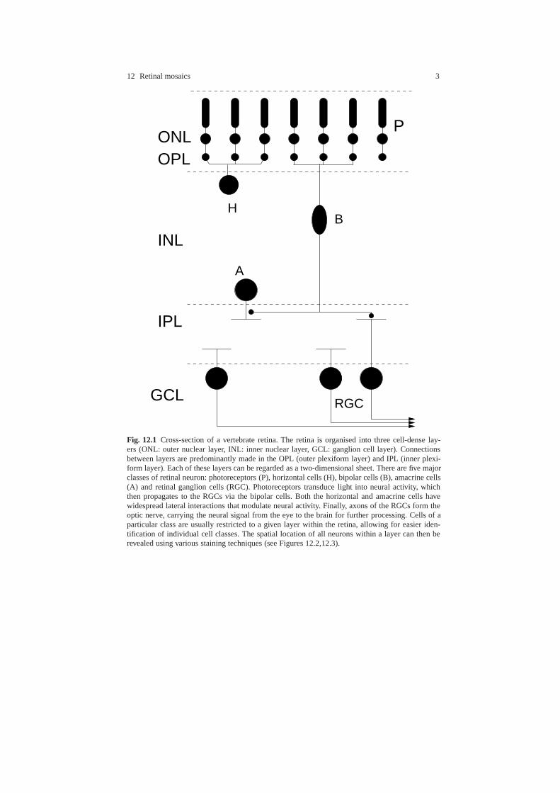
Fig. 12.1 Cross-section of a vertebrate retina. The retina is organised into three cell-dense lay-ers (ONL: outer nuclear layer, INL: inner nuclear layer, GCL: ganglion cell layer). Connectionsbetween layers are predominantly made in the OPL (outer plexiform layer) and IPL (inner plexi-form layer). Each of these layers can be regarded as a two-dimensional sheet. There are five majorclasses of retinal neuron: photoreceptors (P), horizontal cells (H), bipolar cells (B), amacrine cells(A) and retinal ganglion cells (RGC). Photoreceptors transduce light into neural activity, whichthen propagates to the RGCs via the bipolar cells. Both the horizontal and amacrine cells havewidespread lateral interactions that modulate neural activity. Finally, axons of the RGCs form theoptic nerve, carrying the neural signal from the eye to the brain for further processing. Cells of aparticular class are usually restricted to a given layer within the retina, allowing for easier iden-tification of individual cell classes. The spatial location of all neurons within a layer can then berevealed using various staining techniques (see Figures 12.2,12.3).

4 Stephen J. Eglen

Fig. 12.2 Regular arrangement of on-centre alpha retinal ganglion cells from cat retina. The areashown is approximately 1.7×1.2 mm. The dendrites around each cell body tile the retinal surface,and the cell bodies seem roughly equally-spaced from each other. In this article, ’field’ means thearea of tissue within which the neurons are observed. Other neurons (e.g. off-centre alpha retinalganglion cells) within the same layer are not shown. Reproduced by permission from MacmillanPublishers Ltd: Nature 292:344–345, copyright 1981.

Fig. 12.3 Close packing ofcone photoreceptors in a hu-man retina (subject namedMD). The three differentclasses of photoreceptor arecoloured blue (short wave-length), green (mediumwavelength) and red (longwavelength). Approximatewidth of view: 20 arc min.Reproduced from (Hofer et al,2005) with permission of theSociety for Neuroscience.

12 Retinal mosaics 5

index (RI) is simply the mean of this distribution divided by its standard deviation.For the example in Figure 12.4, the RI of 5.1 indicates a highly regular mosaic.

Calculating a measure such as this immediately raises the question of how to in-terpret this number. Cook (1996) first investigated the properties of the RI (termedthe conformity ratio in his article). The baseline to compare against is when theneurons are placed at random throughout the field — this is termed complete spatialrandomness (CSR). The RI for neurons arranged randomly is 1.9, and the more reg-ular the arrangement, the higher the RI. For retinal mosaics observed to date, the RIis typically 3–8. However, the exact threshold for determining whether the mosaicis non-randomly arranged depends on the number of neurons and the geometry ofthe field (Cook, 1996). Furthermore, the physical size of the soma may introducelower limits onto the size of the nearest-neighbour distances. However, all of thesecan be handled appropriately by using Monte-Carlo techniques, see later.

Fig. 12.4 Example mosaic(synthetic data set). Neuronsare drawn as circles with10 µm diameter representingtypical soma size; scale bar:100 µm. Each neuron issurrounded by its Voronoipolygon, showing the regionof space closest to that point.The histogram underneathshows the distribution ofnearest-neighbour distances,along with the regularityindex (RI) of 5.1. This RI istypical of regular mosaics,such as cholinergic amacrineneurons. Nearest neighbour (µm)

Fre

quen

cy

0 20 40 60 80 100

05

10152025

mean 51.7 µmsd 10.2 µmRI 5.1

6 Stephen J. Eglen

12.2.2 Autocorrelation methods

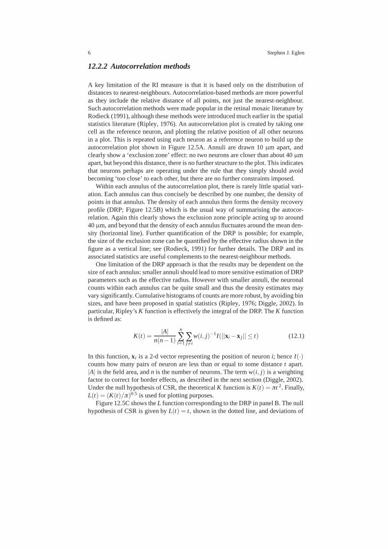
A key limitation of the RI measure is that it is based only on the distribution ofdistances to nearest-neighbours. Autocorrelation-based methods are more powerfulas they include the relative distance of all points, not just the nearest-neighbour.Such autocorrelation methods were made popular in the retinal mosaic literature byRodieck (1991), although these methods were introduced much earlier in the spatialstatistics literature (Ripley, 1976). An autocorrelation plot is created by taking onecell as the reference neuron, and plotting the relative position of all other neuronsin a plot. This is repeated using each neuron as a reference neuron to build up theautocorrelation plot shown in Figure 12.5A. Annuli are drawn 10 µm apart, andclearly show a ‘exclusion zone’ effect: no two neurons are closer than about 40 µmapart, but beyond this distance, there is no further structure to the plot. This indicatesthat neurons perhaps are operating under the rule that they simply should avoidbecoming ‘too close’ to each other, but there are no further constraints imposed.

Within each annulus of the autocorrelation plot, there is rarely little spatial vari-ation. Each annulus can thus concisely be described by one number, the density ofpoints in that annulus. The density of each annulus then forms the density recoveryprofile (DRP; Figure 12.5B) which is the usual way of summarising the autocor-relation. Again this clearly shows the exclusion zone principle acting up to around40 µm, and beyond that the density of each annulus fluctuates around the mean den-sity (horizontal line). Further quantification of the DRP is possible; for example,the size of the exclusion zone can be quantified by the effective radius shown in thefigure as a vertical line; see (Rodieck, 1991) for further details. The DRP and itsassociated statistics are useful complements to the nearest-neighbour methods.

One limitation of the DRP approach is that the results may be dependent on thesize of each annulus: smaller annuli should lead to more sensitive estimation of DRPparameters such as the effective radius. However with smaller annuli, the neuronalcounts within each annulus can be quite small and thus the density estimates mayvary significantly. Cumulative histograms of counts are more robust, by avoiding binsizes, and have been proposed in spatial statistics (Ripley, 1976; Diggle, 2002). Inparticular, Ripley’s K function is effectively the integral of the DRP. The K functionis defined as:

K(t) =|A|

n(n− 1)

n

∑i=1∑j �=i

w(i, j)−1I(||xi − x j|| ≤ t) (12.1)

In this function, xi is a 2-d vector representing the position of neuron i; hence I(·)counts how many pairs of neuron are less than or equal to some distance t apart.|A| is the field area, and n is the number of neurons. The term w(i, j) is a weightingfactor to correct for border effects, as described in the next section (Diggle, 2002).Under the null hypothesis of CSR, the theoretical K function is K(t) = πt 2. Finally,L(t) = (K(t)/π)0.5 is used for plotting purposes.

Figure 12.5C shows the L function corresponding to the DRP in panel B. The nullhypothesis of CSR is given by L(t) = t, shown in the dotted line, and deviations of

12 Retinal mosaics 7

L(t) below that line indicate regularity, as is the case here. (L(t)> t would indicatethat the neurons are clustered, rather than spaced-apart.)

Many other statistics are also available, including Voronoi-based measures, aswell as other cumulative distance functions from the spatial statistics literature (no-tably the F and G functions); for further details, see (Diggle, 2002). It is an openquestion as to which of these functions are most useful for discriminating patterns,hence it is good practice to compare the effectiveness of several functions.

Fig. 12.5 Autocorrelation-based analysis of the mosaicshown in Figure 12.4. A:autocorrelation plot. Each dotrepresents the position of acell relative to another neuronin the field. Annuli are spaced10 µm apart. The lack ofcells in the first four annuliindicate the presence of anexclusion zone. B: densityrecovery profile (DRP). Eachbar in the histogram showsthe density of points in thecorresponding annulus ofthe autocorrelation plot. Thehorizontal line indicates themean density of points (166cells/mm2) and the verticalline (at 38 µm) shows theeffective radius (see text). C:The L function is the scaledintegral of the DRP. Solidline indicates the L functionfor the mosaic; dotted lineindicates the curve that wouldbe expected if the points werearranged randomly.

Distance (µm)

Den

sity

(m

m−2

)

0

50

100

150

200

0 100|

0 20 40 60 80 100

0

20

40

60

80

100

Distance (µm)

L

A

B

C

8 Stephen J. Eglen

12.2.3 Boundary effects

Fig. 12.6 Demonstration ofboundary effects. The solidrectangle indicates the bound-ary region under study, with acentral safety zone shown asdotted lines. Individual points(1, 2, a, b and c) are referredto in the text.

12

ac

b

Figure 12.6 demonstrates the problems associated with boundary effects whenquantifying retinal mosaics. For example, when finding the nearest neighbours, forcells in the centre of the region (e.g. cell 1) it is clear which cell is the nearestneighbour (cell 2). However, for a cell close to the boundary, such as cell a, althoughcell b is the closest within the field, there might have been another cell just to theright of the field that was closer to cell a (e.g. at point c or anywhere within thecircle outside the field). Hence the estimate of the nearest neighbour for cells at theborder is unreliable. To determine which cells are located at the border, we can adda ‘safety zone’, marked by the dotted line, and consider only the nearest-neighbourdistances for neurons within the safety zone (filled symbols). However, what size ofsafety zone should be imposed? The larger the safety zone around the edge of thefield, the smaller the impact of boundary cells. With larger safety zones however,fewer neurons are left within the safety region, and hence fewer samples to estimatethe RI.

Imposing a safety zone is therefore simple, but requires another parameter (thewidth of the safety zone) and often discards a lot of data. Another technique foridentifying border cells is to use the Voronoi tessellation, and label neurons as beingat the border if their Voronoi polygon intersects with the field boundary. However, asubtler approach to handling boundary effects is to use weighting factors such that acontribution of e.g. each nearest-neighbour distance is measured, but the distancesare weighted according to how close a neuron is to the border. One such edge-correction technique is to measure the fraction of the circumference of a circle (e.g.shown for point a in Figure 12.6) that lies within the field (Ripley, 1976; Diggle,2002). This edge-correction term accounts for the w(i, j) term in equation 12.1.

Another concern with boundary procedures that is often overlooked is the size ofthe field itself. Often, retinal mosaics are described simply by the x,y locations ofeach neuron — the coordinates of the (usually rectangular) field which determinewhich neurons are recorded are often not kept. As seen above, the position of theboundary is important, and affects the reliability of the measures taken from themosaic. In the absence of a reported boundary region, one can be estimated by using

12 Retinal mosaics 9

the extreme x and y coordinates of all the neurons. This is the smallest possible field,and although it is the maximum likelihood estimate (Ripley and Rasson, 1977), it isobviously an underestimate.

Ideally therefore, the field is decided in advance, placed onto the retinal tissue,and the positions of all neurons within that field should be recorded. What sizeshould the field be? For practical purposes, most software assumes rectangular re-gion (although some, such as SPLANCS (Rowlingson and Diggle, 1993) can handlearbitrary closed polygons). It should also be large enough to contain enough cells(e.g. at least 50), but small enough so that long-range spatial variations in densitycan be ignored. Again, some methodologies exist for handling non-homogeneitiesin spatial density across the field (Baddeley and Turner, 2005). However, often thelong-range density variations observed across the retinal surface mean that investi-gators do not use very large fields, typically smaller than 1 mm × 1 mm.

12.3 Phenomenological approaches to modelling

What are the mechanisms underlying the development of these retinal mosaics?Progenitors of retinal neurons divide at the location of the photoreceptor layer, andonce the neurons become postmitotic (i.e. stop dividing), they migrate through theretina to the appropriate layer for a given cell type. Certain cell types then migratelaterally within a layer to reach their final position (Reese and Galli-Resta, 2002).As well as these migratory processes, many other developmental mechanisms arethought to be involved, including lateral inhibition of cell fate and cell death (Reeseand Galli-Resta, 2002). For a general review of the developmental mechanisms, seeCook and Chalupa (2000).

In addition to experimental approaches to understanding mosaic formation, theo-retical modelling can help us evaluate the potential of different developmental mech-anisms for generating such regular patterns. In this chapter I compare two styles ofmodelling:

phenomenological the focus is on generating model output that looks similar toobserved data, using mechanisms that may or may not be biologically plausible.

mechanistic the primary concern is on modelling the cellular processes thoughtto be involved, rather than focusing on model output.

These two approaches are common in areas of biological modelling (e.g. seeNathan and Muller-Landau (2000)). In this section, I describe the phenomenologicalapproaches; mechanistic approaches are discussed in the following section.

10 Stephen J. Eglen

12.3.1 Exclusion zone models

The exclusion zone model is fairly straightforward and simply embodies the lo-cal rule that no two neurons should come closer to each other than some minimaldistance. This local exclusion zone should then be able to recreate the hole seenin autocorrelation plots. This style of model was first applied to retinal mosaics byShapiro et al (1985), who examined the spatial distribution of blue cone photorecep-tors in macaque retinas. However, the exclusion zone model has been popularised bythe more recent work of Galli-Resta and colleagues (Galli-Resta et al, 1997), wherethe model is termed the dmin model, where dmin is the main parameter of the model,representing the diameter of the exclusion zone. The value of d min is normally notfixed, but drawn from a normal distribution with a given mean and standard devia-tion. The other parameters of the model (the field size and the number of cells) aretaken from the observed mosaic being modelled.

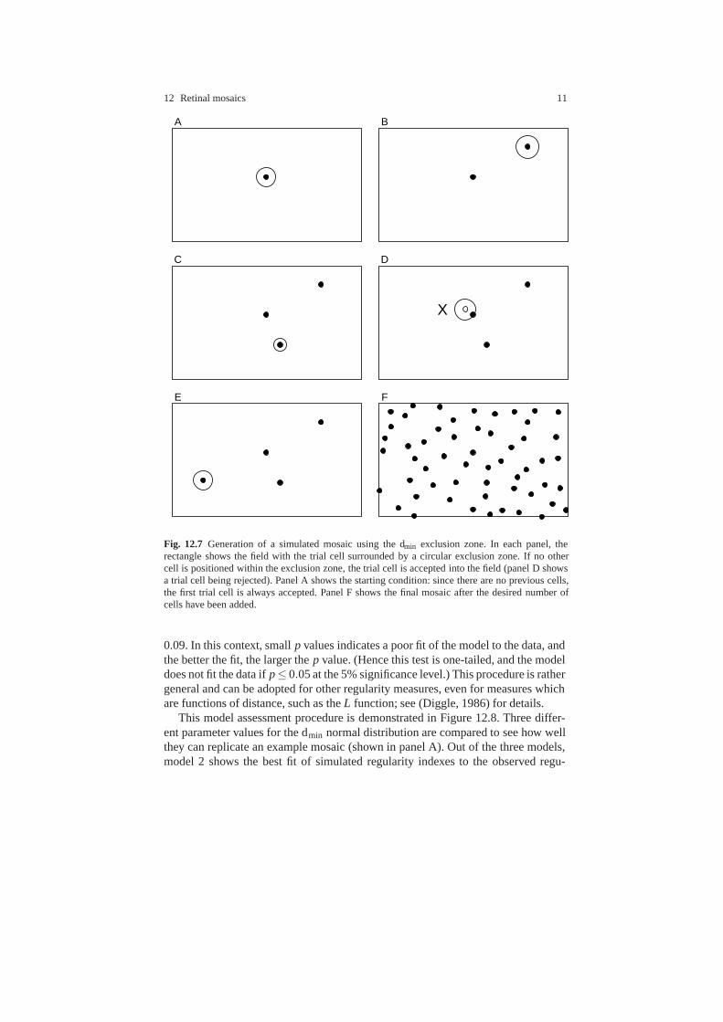
The dmin model is an example of a serial model, where neurons are positionedone-by-one into the field (Figure 12.7). The starting point therefore is an emptyfield, the same size as the mosaic being modelled. A trial point is selected at randomwithin the field, and a value for dmin is sampled from the normal distribution. If thenearest-neighbouring neuron in the field is closer than d min, the trial cell is rejected,otherwise the trial cell is added into the field. This process continues until either thedesired number of neurons have been added into the field or until it is no longerpossible to fit any more neurons.

Once a field has been simulated using the dmin model, it can be compared againstthe observed mosaic (Figure 12.8). Visual comparisons are often inadequate, andso we use the quantitative methods (outlined in Section 12.2) to compare observedwith simulated mosaics. We take advantage of the fact that we can generate manyinstances of simulated mosaics to estimate the goodness of fit. For example, if weuse the RI as the metric to quantify regularity, we calculate the RI of the observedmosaic and the RI of each of 99 simulated mosaics from the d min model (fixingthe parameter values, and just varying the random number generator for positioningneurons). Informally, for a good fit, the RI of the observed mosaic should fall withinthe range of RIs generated by the dmin model.

This assessment of goodness of fit can then be quantified by calculating an em-pirical p value. If the RI of the observed mosaic is x1 and the RI of n− 1 simulatedmosaics are x2 . . .xn, then for each mosaic i we calculate a ui value which determinesthe difference between the RI for mosaic i and the average RI of all other mosaics:

ui = abs

(xi − 1

n− 1 ∑j �=i

x j

)

The expectation then is that if the model is a good fit to the data, u 1 should be ofsimilar magnitude to all other u scores. A p value can then be calculated by sortingthe values of u, largest first, and then counting the position of u 1 and dividing by n.For example, if u1 was the ninth largest value of u out of 100, the p value would be

12 Retinal mosaics 11

A B

C

X

D

E F

Fig. 12.7 Generation of a simulated mosaic using the dmin exclusion zone. In each panel, therectangle shows the field with the trial cell surrounded by a circular exclusion zone. If no othercell is positioned within the exclusion zone, the trial cell is accepted into the field (panel D showsa trial cell being rejected). Panel A shows the starting condition: since there are no previous cells,the first trial cell is always accepted. Panel F shows the final mosaic after the desired number ofcells have been added.

0.09. In this context, small p values indicates a poor fit of the model to the data, andthe better the fit, the larger the p value. (Hence this test is one-tailed, and the modeldoes not fit the data if p≤ 0.05 at the 5% significance level.) This procedure is rathergeneral and can be adopted for other regularity measures, even for measures whichare functions of distance, such as the L function; see (Diggle, 1986) for details.

This model assessment procedure is demonstrated in Figure 12.8. Three differ-ent parameter values for the dmin normal distribution are compared to see how wellthey can replicate an example mosaic (shown in panel A). Out of the three models,model 2 shows the best fit of simulated regularity indexes to the observed regu-

12 Stephen J. Eglen

larity index. This is confirmed by computing the u scores and p values. Clearly,quantitative methods are required for comparing observed data and model output,as there are no strong visual differences among the three alternative models shownin Figure 12.8B–D.

Finally, Figure 12.9 shows the p values obtained by this procedure for a rangeof different model parameters. As the dmin model is relatively fast, such exhaustiveparameter searches are feasible, and can easily pinpoint parts of parameter spacewhere the model fits the data. For more complex models, an exhaustive approach isnot feasible, and instead a heuristic search procedure should be used. Some otherphenomenological models from the spatial statistics literature have specialised fit-ting procedures – for example see the R package SPATSTAT for details (Baddeleyand Turner, 2005).

Evaluation of dmin model

The dmin model has been used to fit a wide range of mosaics of different cell typesand different species (Galli-Resta et al, 1997, 1999; Cellerino et al, 2000; Ravenet al, 2003). This strongly suggests that a homotypic exclusion zone is sufficient togenerate a retinal mosaic. (In this context, homotypic means that interactions arerestricted to cells of the same type; heterotypic interactions involve cells of dif-ferent types.) This means it is unlikely that long-range interactions are requiredbetween cells of the same type, nor are interactions needed between cells of differ-ent types, confirming results from cross-correlation analysis (Rockhill et al, 2000;Mack, 2007). However, the dmin model does not say anything about the biologicalmechanisms underlying the generation of such local exclusion zones. I return to thistopic in section 12.4.

12.3.2 Other phenomenological models

The dmin model is one instantiation of a whole class of phenomenological modelswhereby spatial points exhibit mutual exclusion (Diggle, 2002). A generalisation ofthis style of model is the pairwise interaction point process whereby a non-negativefunction h(t) influences the probability of any two cells being a distance t apart. Theshape of h(t) can then determine both excitatory and inhibitory interactions betweenpairs of points, as demonstrated by Diggle (2002). These models also allow fora ‘birth-and-death’ style of cell positioning: cells are initially positioned randomlywithin the field, and then individual cells are killed and move to new positions. Suchbirth-and-death algorithms need several iterations to converge, but are preferable tothe serial methods which may introduce order artifacts (cells added later into thefield are more difficult to position than earlier-born cells). For further details see(Diggle, 2002; Eglen et al, 2005).

12 Retinal mosaics 13

data model 1: dmin N(16,2)

model 2: dmin N(21,6) model 3: dmin N(20,10)

2 3 4 5 6 7regularity index

0.0 0.5 1.0 1.5U score

model 1p=0.01

model 2p=0.96

model 3p=0.01

A B

C D

E F

Fig. 12.8 Fitting the dmin model to an example mosaic. A: example observed mosaic (cholinergicamacrine cells in rat). The field of view is 400×400 µm2. B–D: example simulations using threedifferent values for dmin parameters; in each case the dmin value is drawn from a normal distributionwith given mean and s.d. E–F: assessing the fit of each model to the data. In E, each row showsthe regularity index from 99 simulations of each model; the larger vertical line in each case is theregularity of the observed data in A (4.16). Informally, the model fits the data if the observed RIfalls within the range of the RIs generated by the model. Panel F shows the u score for each mosaic(real or simulated), with the score for the real mosaic drawn with a larger line. Whereas model 1and 3 can be rejected, model 2 fits the data.

14 Stephen J. Eglen

mean (µm)

s.d.

(µ

m)

15 16 17 18 19 20 21 22 23 24 25

2

4

6

8

10

Fig. 12.9 Exhaustive parameter search of the dmin model to fit the observed mosaic shown in Fig-ure 12.8A. For each value of the mean and s.d. of the dmin model, 99 simulations were generated,and the p value for comparing real and simulated mosaics obtained. The area of the square in eachcase is proportional to the p value.

Finally, in contrast to the models whereby local order emerges from randominitial conditions, another class of model has been proposed for modelling retinalmosaics whereby an initially regular hexagonal mosaic is distorted to match theobserved pattern. This ‘distorted lattice’ approach has been used to model the dis-tribution of horizontal cells (Ammermuller et al, 1993) and retinal ganglion cells(Zhan and Troy, 2000). Although these models can recreate the spatial propertiesof observed retinal mosaics, they are of limited utility in informing us about the de-velopmental mechanisms underlying mosaic generation as they require hexagonalmosaics to be first created and then distorted.

12.4 Mechanistic models

In this section I briefly discuss mechanistic models that have been proposed forgeneration of retinal mosaics. The key focus of these models is to help further un-derstand the developmental mechanisms underlying pattern formation, as opposedto observing a good statistical fit between model and data. For further details ofthese models, the reader is referred to the original references and (Eglen, 2006).

12 Retinal mosaics 15

12.4.1 Lateral migration

Once retinal neurons become postmitotic, they migrate radially through the layers ofthe retina until they arrive at the layer that is appropriate for their cell type. Whilstthey migrate through the layers, it is thought that cells of the same type do notrespect any minimal spacing rule (Galli-Resta et al, 1997). They therefore arriverandomly spaced over a period of several days. However, once they arrive in thedestination layer, they appear to move laterally within the layer. The amount oflateral movement observed varies by cell type (Reese et al, 1999), and those thatmove more tend to have more regular mosaics.

What causes the lateral movement of neurons within their destination layer?Early evidence suggested a correlation between the time of movement and the firstemergence of neurites in horizontal cells (Reese et al, 1999). This suggested thatdendritic interactions might underlie the lateral migration, a hypothesis that wasinvestigated using modelling techniques (Eglen et al, 2000), described in the nextparagraph. Subsequently, further evidence for the role of dendritic interactions inmosaic formation came from work by Galli-Resta showing that temporary disrup-tion of microtubules in dendrites caused mosaics to collapse; once microtubule func-tion restored, mosaic organization returned (Galli-Resta et al, 2002). Most recently,mosaics are disrupted in mice lacking the cell adhesion molecule DSCAM, possi-bly as a consequence of altered dendritic fasciculation among homotypic neurons(Fuerst et al, 2008).

In the lateral migration model (Eglen et al, 2000), neurons initially have smallcircular dendritic arbors. Each cell receives input from its neighbours in propor-tion to the amount of dendritic overlap, and arbor size varies to maintain a fixedamount of input from neighbouring cells (van Ooyen and van Pelt, 1994). In addi-tion, cells repel each other in proportion to their dendritic overlap. In this manner, asdendritic arbors develop, cells gradually begin to repel each other; once arbor sizeshave stabilised, the cells then gradually settle into a regular hexagonal-like mosaiclayout. The amounts that each cell moves is small, in line with the lateral distancesobserved experimentally (Reese et al, 1999). One limitation of the model is that itusually generates mosaics with regularity indexes that are much higher than thoseobserved experimentally. This is because the model dendrites are perfectly circularand the amount of overlap between arbors is calculated exactly. Reducing the preci-sion with which the amount of overlap is detected produces more realistic mosaics(Eglen et al, 2000). Subsequent modelling work has also examined in detail the me-chanical forces that might compose the dendritic interactions, thus moving towardsmore realistic description of the developing dendrites (Ruggiero et al, 2004).

12.4.2 Lateral inhibition of cell fate

The eventual identity of any given neuron in the retina is not predetermined early indevelopment but is influenced by many intrinsic and environmental factors during

16 Stephen J. Eglen

development. Many cell fate mechanisms influence the identity of a given cell. Oneof the most common is lateral inhibition: neighbouring neurons compete to inhibiteach other from acquiring a particular fate. There are many molecular pathways bywhich this lateral inhibition is mediated, but most notable is that of Delta-Notchsignalling (Frankfort and Mardon, 2002). Cell fate mechanisms can therefore nat-urally impose minimal distance constraints as they prevent neighbours from beingthe same type of neuron.

The effect of cell fate interactions upon the relative numbers of primary and sec-ondary fate neurons was studied by Honda et al (1990). This early modelling studyshowed that lateral inhibitory mechanisms are sufficient to generate the correct rel-ative numbers of primary and secondary fate neurons in developing grasshopperneuroblasts. We have subsequently shown that lateral inhibition can generate reg-ular primary fate mosaics from an initial irregular distribution of undifferentiatedneurons (Eglen and Willshaw, 2002). However, if the initial population of undiffer-entiated neurons is already regular, the subsequent mosaic of primary fate neuronsis not more regular than the initial population. Stochastic cell fate processes havealso been shown theoretically to be sufficient to account for the generation of reg-ular mosaics in zebrafish photoreceptors (Tohya et al, 1999). Further work by thisgroup showed that these zebrafish mosaics could equivalently be generated by cellrearrangement processes (Mochizuki, 2002; Tohya et al, 2003).

12.4.3 Cell death

Many more neurons are produced in development than survive to adulthood. Forexample, estimates suggest that 50–90% of RGCS that are born will die beforeadulthood (Finlay and Pallas, 1989). This programmed cell death may have manyroles in development, including the refinement of retinal projections to their targets(O’Leary et al, 1986). Cell death might be an active process in forming retinal mo-saics, by removing those inappropriately-positioned neurons that are too close totheir neighbours (Jeyarasasingam et al, 1998; Cook and Chalupa, 2000). The mech-anisms by which neurons detect that they are too close too each other are howeverunknown. Furthermore, computer modelling of this process suggests that the celldeath would need to be highly selective or the level of cell death would need to bevery high to transform an irregular mosaic into a regular mosaic (Eglen and Will-shaw, 2002). These modelling studies would therefore suggest that cell death alonedoes not account for the emergence of RGC mosaics (Jeyarasasingam et al, 1998).Cell death could however account for the generation of other mosaics, e.g. dopamin-ergic amacrine neurons (Raven et al, 2003), as the level of naturally-occurring celldeath is very high and the final mosaics are only mildly regular.

12 Retinal mosaics 17

12.4.4 Interactions between developmental mechanisms

Although cell death alone could not account for the emergence of RGC mosaics,it is likely that many mechanisms can co-operate to generate regular mosaics. In-deed, combining lateral inhibition of cell fate with cell death is sufficient to gen-erate highly regular RGC-like mosaics (Eglen and Willshaw, 2002). The effects ofinteractions between several developmental mechanisms has been studied withinthe context of cellular patterns in the chick inner ear, the basilar papilla (Goodyearand Richardson, 1997), where primary fate cells are regularly distributed across thesurface (Podgorski et al, 2007). Three different mechanisms were studied: lateralinhibition of cell fate, cell death, and differential adhesion. Individually, no singlemechanism could account for the generation of the primary fate mosaics. However,iteratively coupling these mechanisms robustly generated regular patterns over awide range of initial conditions. These results suggest that modelling the interac-tions between developmental mechanisms is clearly important before one can fullyunderstand the relative role of individual processes, such as cell death.

12.5 Exclusion zone modelling: application to two types ofneuron

This previous section has outlined several mechanisms that could underlie the gener-ation of retinal mosaics, and in particular how an exclusion zone might be generated.If we assume that exclusion zones can somehow be generated, then it is natural toreturn to the dmin model and see how else it can be used to investigate mosaic forma-tion. In particular, in this section we consider whether the dmin model can accountfor the generation of cellular patterns involving two related cell types.

Out of the 60+ cell types in the retina, there are several types of cell that come incomplementary pairs (Cook and Chalupa, 2000). For example, the most prominentexample of complementary pairing is the classification of alpha and beta RGCs intotwo types: on-centre or off-centre, depending on their response to light (Wassle et al,1981a,b). Likewise, in both cat and macaque, horizontal cells are divided into twotypes, each regularly arranged (Wassle et al, 1978, 2000). In this section I show howexclusion zone modelling can test whether heterotypic developmental interactionsare required to generate these mosaics.

Figure 12.10A shows the regular arrangement of two types of horizontal cell inmacaque (Wassle et al, 2000). There are roughly twice as many type 1 neuronsas type 2 neurons. The regularity index for all neurons (irrespective of type) is justunder 4.0 (Figure 12.11), which is relatively high and thus lead to the suggestion thatthe two types of neuron might interact to create this high regularity (Wassle et al,2000). To test this hypothesis, we extended the exclusion zone model to include twotypes of neurons (Eglen and Wong, 2008). Each neuron respected the exclusion zoneonly of cells of the same type; the only interaction between cells of different type

18 Stephen J. Eglen

H1H2

A B

Fig. 12.10 Regular arrangement of two types of horizontal cells. A: observed distribution frommacaque retina. Type 1 neurons are drawn as open circles, type 2 cells are filled. B: example outputfrom the extended dmin model, assuming no interactions between cell types except for preventingsomal overlap.

was that they could not come closer than about 12 µm, the average soma diameter, toprevent somal overlap. This model generated retinal mosaics that were both visually(Figure 12.10B) and quantitatively similar, as assessed by distribution of regularityindexes (Figure 12.11) and L functions (Eglen and Wong, 2008). Thus, the exclusionzone model predicts that horizontal cell mosaics can emerge without heterotypicinteractions. A similar conclusion was reached for the generation of two types ofbeta RGCs in cat, using a more flexible exclusion zone technique (Eglen et al, 2005).

Fig. 12.11 Quantitative com-parison of the extended dminmodel with the macaquehorizontal cells. The hori-zontal grey line shows theobserved regularity index foreither type 1 neurons, type2 neurons, or all neurons,irrespective of type. Blackdots indicate the regularityindex from 99 simulations.The observed regularity indexfalls within the range of the99 simulations, indicating agood fit between model anddata.

1 2 1+2

regu

larit

y in

dex

2

4

6

cell type

12 Retinal mosaics 19

12.6 Future directions

The retina is an ideal system for investigating questions of cellular patterning forseveral reasons. First, there is a comprehensive catalogue of individual retinal celltypes (Masland, 2004), and although the number of cells seems large (60+), it is pre-sumably much smaller than in other parts of the nervous system. Second, most cellsof an individual type are located at a single depth within the retina, reducing theproblem of cellular arrangements from three- to two-dimensions. Third, there areseveral selective neurochemical markers available to reliably stain individual celltypes. (However, most of these markers only work reliably in adulthood, rather thanearly in development.) To see whether the principles of cellular organisation gener-alise from the retina to other parts of the central nervous system, several experimen-tal challenges must be overcome. For example, we need reliable techniques for iden-tifying and labelling individual cell types. Moving from two- to three-dimensionalspace will require accurate reconstruction within a volume (Oberlaender et al, 2009).By contrast, most of the theoretical techniques should generalise from the retina toother parts of the CNS (e.g. (Prodanov and Feirabend, 2007; Prodanov et al, 2007))and into three dimensions (Baddeley et al, 1993). Most of the computational toolsare also freely available in either Matlab or R (Rowlingson and Diggle, 1993; Bad-deley and Turner, 2005; Eglen et al, 2008). Finally, aside from investigating devel-opmental mechanisms, the analysis of spatial patterning of neurons in adulthood isalso important in several clinical contexts (Diggle et al, 1991; Cotter et al, 2002;Lei et al, 2009). There has been relatively little modelling of spatial patterning inthese clinical contexts, but as the technical limitations described above are over-come, I hope that computational modelling will be a useful tool in understandingthe generation and perturbation of these patterns.

Acknowledgements This work was supported by funding from the Wellcome Trust and NIH.Experimental data kindly provided by Dr Lucia Galli-Resta and Prof Heinz Wassle. Thanks toAndreas Lønborg for comments on a draft version of this chapter.

12.7 Further Reading

• Statistical analysis of spatial point patterns (Diggle, 2002). This is a short butcomprehensive description of most of the key techniques described in this chap-ter.

• Principles of computational modelling in neuroscience (Sterratt et al, 2011).Comprehensive textbook on modelling neural systems, including a chapter onneural development.

• Retinal development (Sernagor et al, 2006). Edited collection of articles describ-ing the different stages of vertebrate retinal development.

20 Stephen J. Eglen

References

Ammermuller J, Mockel W, Rugan P (1993) A geometrical description of horizontalcell networks in the turtle retina. Brain Research 616:351–356

Baddeley A, Turner R (2005) Spatstat: an R package for analyzing spatial pointpatterns. J Stat Software 12:1–42

Baddeley AJ, Moyeed RA, Howard CV, Boyde A (1993) Analysis of a three-dimensional point pattern with replication. Appl Stats 42:641–668, DOI10.2307/2986181

Cellerino A, Novelli E, Galli-Resta L (2000) Retinal ganglion cells with NADPH-diaphorase activity in the chick form a regular mosaic with a strong dorsoventralasymmetry that can be modelled by a minimal spacing rule. European Journal ofNeuroscience 12:613–620

Cook JE (1996) Spatial properties of retinal mosaics: an empirical evaluation ofsome existing measures. Visual Neuroscience 13:15–30

Cook JE (1998) Getting to grips with neuronal diversity. In: Chaulpa LM, FinlayBL (eds) Development and organization of the retina, Plenum Press, pp 91–120

Cook JE, Chalupa LM (2000) Retinal mosaics: new insights into an old concept.Trends in Neuroscience 23:26–34

Cotter D, Mackay D, Chana G, Beasley C, Landau S, Everall I (2002) Reducedneuronal size and glial cell density in area 9 of the dorsolateral prefrontal cortexin subjects with major depressive disorder. Cereb Cortex 12:386–394

Diggle P, Lange N, Benes F (1991) Analysis of variance for replicated spatial pointpatterns in clinical neuroanatomy. Journal of the American Statistical Association86:618–625

Diggle PJ (1986) Displaced amacrine cells in the retina of a rabbit: analysis of abivariate spatial point pattern. J Neurosci Methods 18:115–125

Diggle PJ (2002) Statistical analysis of spatial point patterns, 2nd edn. London:Edward Arnold

Eglen SJ (2006) Development of regular cellular spacing in the retina: theoreticalmodels. Math Med Biol 23:79–99

Eglen SJ, Willshaw DJ (2002) Influence of cell fate mechanisms upon retinal mosaicformation: a modelling study. Development 129:5399–5408

Eglen SJ, Wong JCT (2008) Spatial constraints underlying the retinal mosaics oftwo types of horizontal cells in cat and macaque. Visual Neuroscience 25:209–214

Eglen SJ, van Ooyen A, Willshaw DJ (2000) Lateral cell movement driven by den-dritic interactions is sufficient to form retinal mosaics. Network: Computation inNeural Systems 11:103–118

Eglen SJ, Diggle PJ, Troy JB (2005) Homotypic constraints dominate positioningof on- and off-centre beta retinal ganglion cells. Visual Neuroscience 22:859–871

Eglen SJ, Lofgreen DD, Raven MA, Reese BE (2008) Analysis of spatial relation-ships in three dimensions: tools for the study of nerve cell patterning. BMC Neu-roscience 9:68

12 Retinal mosaics 21

Finlay BL, Pallas SL (1989) Control of cell number in the developing mammalianvisual system. Prog Neurobiol 32:207–234

Frankfort BJ, Mardon G (2002) R8 development in the drosophila eye: a paradigmfor neural selection and differentiation. Development 129:1295–1306

Fuerst PG, Koizumi A, Masland RH, Burgess RW (2008) Neurite arborization andmosaic spacing in the mouse retina require DSCAM. Nature 451:470–474

Galli-Resta L (2002) Putting neurons in the right places: local interactions in thegenesis of retinal architecture. Trends in Neuroscience 25:638–643

Galli-Resta L, Resta G, Tan SS, Reese BE (1997) Mosaics of Islet-1-expressingamacrine cells assembled by short-range cellular interactions. Journal of Neuro-science 17:7831–7838

Galli-Resta L, Novelli E, Kryger Z, Jacobs GH, Reese BE (1999) Modelling themosaic organization of rod and cone photoreceptors with a minimal-spacing rule.European Journal of Neuroscience 11:1461–1469

Galli-Resta L, Novelli E, Viegi A (2002) Dynamic microtubule-dependent interac-tions position homotypic neurones in regular monolayered arrays during retinaldevelopment. Development 129:3803–3814

Goodyear R, Richardson G (1997) Pattern formation in the basilar papilla: evidencefor cell rearrangement. Journal of Neuroscience 17:6289–6301

Hofer H, Carroll J, Neitz J, Neitz M, Williams DR (2005) Organization of the humantrichromatic cone mosaic. Journal of Neuroscience 25:9669–9679

Honda H, Tanemura M, Yoshida A (1990) Estimation of neuroblast numbers ininsect neurogenesis using the lateral inhibition hypothesis of cell differentiation.Development 110:1349–1352

Jeyarasasingam G, Snider CJ, Ratto GM, Chalupa LM (1998) Activity-regulatedcell death contributes to the formation of on and off alpha ganglion cell mosaics.Journal of Comparative Neurology 394:335–343

Lei Y, Garrahan N, Hermann B, Fautsch M, Hernandez MR, Boulton M, MorganJE (2009) Topography of neuron loss in the retinal ganglion cell layer in humanglaucoma. Br J Ophthalmol 93:1676–1679, DOI 10.1136/bjo.2009.159210

Mack AF (2007) Evidence for a columnar organization of cones, Muller cells, andneurons in the retina of a cichlid fish. Neuroscience 144:1004–1014

Masland RH (2004) Neuronal cell types. Curr Biol 14:R497–R500, DOI10.1016/j.cub.2004.06.035

Mochizuki A (2002) Pattern formation of cone mosaic in the zebrafish retina: a cellrearrangement model. Journal of Theoretical Biology 215:345–361

Nathan R, Muller-Landau HC (2000) Spatial patterns of seed dispersal, their deter-minants and consequences for recruitment. Trends Ecol Evol 15:278–285

Oberlaender M, Dercksen VJ, Egger R, Gensel M, Sakmann B, Hege HC (2009)Automated three-dimensional detection and counting of neuron somata. J Neu-rosci Methods 180:147–160

O’Leary DDM, Fawcett JW, Cowan WM (1986) Topographic targeting errors in theretinocollicular projection and their elimination by ganglion cell death. Journalof Neuroscience 6:3692–3705

22 Stephen J. Eglen

van Ooyen A, van Pelt J (1994) Activity-dependent outgrowth of neurons and over-shoot phenomena in developing neural networks. Journal of Theoretical Biology167:27–43

Podgorski GJ, Bansal M, Flann NS (2007) Regular mosaic pattern development: Astudy of the interplay between lateral inhibition, apoptosis and differential adhe-sion. Theor Biol Med Model 4:43

Prodanov D, Feirabend HKP (2007) Morphometric analysis of the fiber populationsof the rat sciatic nerve, its spinal roots, and its major branches. J Comp Neurol503:85–100, DOI 10.1002/cne.21375

Prodanov D, Nagelkerke N, Marani E (2007) Spatial clustering analysis in neu-roanatomy: applications of different approaches to motor nerve fiber distribution.J Neurosci Methods 160:93–108, DOI 10.1016/j.jneumeth.2006.08.017

Raven MA, Eglen SJ, Ohab JJ, Reese BE (2003) Determinants of the exclusionzone in dopaminergic amacrine cell mosaics. Journal of Comparative Neurology461:123–136

Reese BE, Galli-Resta L (2002) The role of tangential dispersion in retinal mosaicformation. Progress in Retinal and Eye Research 21:153–168

Reese BE, Necessary BD, Tam PPL, Faulkner-Jones B, Tan SS (1999) Clonal ex-pansion and cell dispersion in the developing mouse retina. European Journal ofNeuroscience 11:2965–2978

Ripley B, Rasson J (1977) Finding the edge of a Poisson forest. J App Prob 14:483–491

Ripley BD (1976) The second-order analysis of stationary point processes. J AppProb 13:255–266

Rockhill RL, Euler T, Masland RH (2000) Spatial order within but not betweentypes of retinal neurons. Proceedings of the National Academy Of Sciences ofthe USA 97:2303–2307

Rodieck RW (1991) The density recovery profile: a method for the analysis of pointsin the plane applicable to retinal studies. Visual Neuroscience 6:95–111

Roorda A, Metha AB, Lennie P, Williams DR (2001) Packing arrangement of thethree cone classes in primate retina. Vision Research 41:1291–1306

Rowlingson BS, Diggle PJ (1993) SPLANCS: spatial point pattern analysis code inS-Plus. Comput Geosci 19:627–655

Ruggiero C, Benvenuti S, Borchi S, Giacomini M (2004) Mathematical model ofretinal mosaic formation. Biosystems 76:113–120

Sernagor E, Eglen SJ, Harris WA, Wong ROL (eds) (2006) Retinal Development.Cambridge University Press

Shapiro MB, Schein SJ, deMonasterio FM (1985) Regularity and structure of thespatial pattern of blue cones of macaque retina. Journal of the American Statisti-cal Association 80:803–812

Sterratt D, Graham B, Gillies A, Willshaw D (2011) Principles of computationalmodelling in neuroscience. Cambridge University Press

Tohya S, Mochizuki A, Iwasa Y (1999) Formation of cone mosaic of zebrafishretina. Journal of Theoretical Biology 200:231–244

12 Retinal mosaics 23

Tohya S, Mochizuki A, Iwasa Y (2003) Difference in the retinal cone mosaic patternbetween zebrafish and medaka: cell-rearrangement model. Journal of TheoreticalBiology 221:289–300

Wassle H (2004) Parallel processing in the mammalian retina. Nat Rev Neurosci5:747–757, DOI 10.1038/nrn1497

Wassle H, Riemann HJ (1978) The mosaic of nerve cells in the mammalian retina.Proceedings of the Royal Society of London Series B 200:441–461

Wassle H, Peichl L, Boycott BB (1978) Topography of horizontal cells in theretina of the domestic cat. Proceedings of the Royal Society of London SeriesB 203:269–291

Wassle H, Boycott BB, Illing RB (1981a) Morphology and mosaic of on-beta andoff-beta cells in the cat retina and some functional considerations. Proceedings ofthe Royal Society of London Series B 212:177–195

Wassle H, Peichl L, Boycott BB (1981b) Morphology and topography of on-alphaand off-alpha cells in the cat retina. Proceedings of the Royal Society of LondonSeries B 212:157–175

Wassle H, Dacey DM, Haun T, Haverkamp S, Grunert U, Boycott BB (2000) Themosaic of horizontal cells in the macaque monkey retina: with a comment onbiplexiform ganglion cells. Visual Neuroscience 17:591–608

Zhan XJ, Troy JB (2000) Modeling cat retinal beta-cell arrays. Visual Neuroscience17:23–39

Index

dmin model, 10

autocorrelation, 6

boundary effects, 8

cell fate, 16complete spatial randomness (CSR), 5

density recovery profile (DRP), 6

exclusion zone model, 10

horizontal cells, 1

lateral inhibition, 16

mechanistic models, 9

phenomenological models, 9photoreceptors, 1

regularity index (RI), 5retinal ganglion cells (RGCs), 1retinal mosaic, 1

Voronoi tessellation, 8

25