Lecture Notes PH 411/511 ECE 598 A. La Rosa Portland State University

INTRODUCTION TO QUANTUM MECHANICS _____________________________________________________________________________________

CHAPTER-11 QUANTUM ENTANGLEMENT The annihilation of the positronium

Except for the “Cartoons Version” presented at the very beginning, and the section “my

own view” given at the very end, this chapter is taken completely from the The Feynman Lectures, Vol III, Chapter 18 and from the book Quantum Mechanics by D. J. Griffiths. The annihilation of the positronium process with the consequent generation of photons is described by Feynman in great detail, accounting for the conservation of energy, linear momentum, angular momentum and parity. Although the word entanglement is not mentioned explicitly, the “Einstein-Podolsky-Rosen paradox” is mentioned in the description. Feynman is on the argument side that states that there is no paradox, and that indeed, measurement on one side affect the result of measurement made at another far away location.

I. CARTOON VERSION: Measurements affected by the actions of a distant observer

II. NON LOCALITY and the QUANTUM THEORY II.1 The EPR paper on the (lack of) Completeness of the Quantum Theory II.2 The Bohm experimental version to settle the EPR paradox

III. The ANNIHILATION of the POSITRONIUM

IV. BELL’S THEOREM

I. CARTOON VERSION: Measurements affected by the actions of a distant observer

1. The figure shows a box with two some peculiar characteristics. Upon shaking the box two particles come out advancing in opposite directions

A

B

Fig. 1. Upon shaking the box, each observer receives a particle.

Based on the results described below, it appears that there are many containers of different colors inside that box (only three colors are shown in the figure). But, actually, it is unknown what exactly is going on inside the mysterious box.

Window Window

Box

Fig. 2. Guess of the possible contents inside the box

2. What is known is that, after shaking the box, two particles leave the box in opposite directions (linear momentum conservation).

The particles are detected, respectively, by two observers A and B.

To determine the color of the balls A and B have to use filters.

A

B

Figure 3. To determine the color of the particles the observer use filters.

3. When both A and B decide, for example, to use only red and blue filters, the following happens:

If one observer selects a given filter (blue for example) and is unable to see the particle then it would imply that the particle is of the opposite color (red).

They call these two colors “basic colors” (Any other color would be a combination of these two)

4. B has decided to use only red or blue filters.

When Observer B uses a blue filter, the result from different trials of shaking the box is that i) sometimes B is able to see a blue particle, ii) sometimes B is unable to see the color of the particle.

Cases i) and ii) occur 50% of the total trials.

5. B has decided to use only red or blue filters. A has decided also to use only red or blue filters.

The following outcome occurs from the observations made by A and B

Upon shaking the box, the figure below displays

two (typically) observed outcomes

A

B

Red Red

(23)

Or

A B

Blue Blue

Fig. 4. Two possible outcomes from the “shaking box” experiment. It appears there is a

“conservation of color” law.

Questions: Do the particles acquire their color before leaving the box?

Could the balls have no color after leaving the box and acquire a color only right after they are detected by A (or by B)?

6. Observer B has decided to use green color filter (one that is not 50% bluish and 50% reddish) to analyze the particle.

A B

Green

filter

Figure 5.

What color particle would A detect?

Will the measurement by A be influenced by what B has done?

An old fashion quantum practitioner would say that, - Observations made by B should NOT affect A’s measurements;

- Whether B makes measurements or not, if A is set to watch the particle with red or blue filters, then, similar to the case depicted in Fig. 3, 50% of the times A will detect a blue color

particle and 50% a red particle.

However, it turns out that, when A uses a red color filter the number of times A sees a read particle is not 50% of the total. Instead, the percentage is closer to the reddish-percentage of the green color filter. That is the prior measurement made by B does affect the post measurement made by A.

A B

Purple

Green

filter

Figure 6.

7. If B does not make any measurement (nor he/she places any filter),

Then, indeed, when A’s detector is set to measure red or blue particles,

50% of the times A will detect a blue color particle and 50% a red particle. From 6 and 7: Measurement made by one observer affect the outcome of the measurement made by the other observer. This occurs because the two particle that come out from the box, constitute an interconnected system as a whole.

II. NON LOCALITY and the QUANTUM THEORY The wave function associated to a physical system does not uniquely determine the

outcome of a measurement; instead it provides a statistical distribution of possible results. Such an interpretation has caused deep controversial discussions.

i) The realistic viewpoint: The physical system has the particular property being measured prior to the act of measurement.

Quantum mechanics is an incomplete theory, for even knowing the wave function, still one cannot determine all the properties of the physical system. Therefore, there is some other information, external to quantum mechanics, which (together with the wave function) is required for a complete description of physical reality.

ii) Orthodox viewpoint: the act of measurement “creates” the property. A measurement forces a system to adopt a given value (corresponding to the the type of

measurement being done). Or equivalently, a measurement makes the wavefunction to collapse into a given stationary state, thus “creating” an attribute on the system that was not there previously.

For example, a two-electron system may be in the state 0S 2/1 [1)( 2)( -

1)( 2)( ]

(where one electron is flying in the opposite direction of the other). Upon using a magnetic field apparatus to measure the spin of the particles, one possible outcome is electron -1 in

the state 1)( and electron-2 in the state

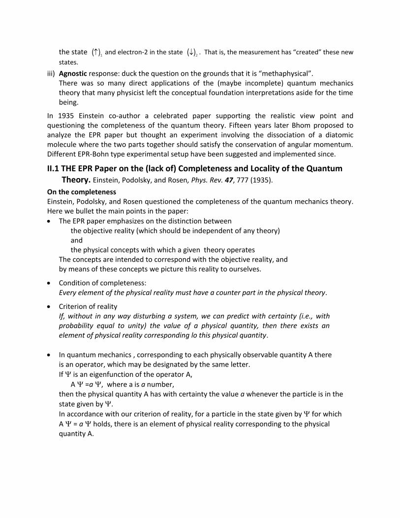
2)( . That is, the measurement has “created” these new

states.

iii) Agnostic response: duck the question on the grounds that it is “methaphysical”. There was so many direct applications of the (maybe incomplete) quantum mechanics

theory that many physicist left the conceptual foundation interpretations aside for the time being.

In 1935 Einstein co-author a celebrated paper supporting the realistic view point and questioning the completeness of the quantum theory. Fifteen years later Bhom proposed to analyze the EPR paper but thought an experiment involving the dissociation of a diatomic molecule where the two parts together should satisfy the conservation of angular momentum. Different EPR-Bohn type experimental setup have been suggested and implemented since.

II.1 THE EPR Paper on the (lack of) Completeness and Locality of the Quantum Theory. Einstein, Podolsky, and Rosen, Phys. Rev. 47, 777 (1935).

On the completeness Einstein, Podolsky, and Rosen questioned the completeness of the quantum mechanics theory. Here we bullet the main points in the paper:

The EPR paper emphasizes on the distinction between the objective reality (which should be independent of any theory) and the physical concepts with which a given theory operates

The concepts are intended to correspond with the objective reality, and by means of these concepts we picture this reality to ourselves.

Condition of completeness: Every element of the physical reality must have a counter part in the physical theory.

Criterion of reality If, without in any way disturbing a system, we can predict with certainty (i.e., with probability equal to unity) the value of a physical quantity, then there exists an element of physical reality corresponding lo this physical quantity.

In quantum mechanics , corresponding to each physically observable quantity A there is an operator, which may be designated by the same letter.

If is an eigenfunction of the operator A,

A =a, where a is a number, then the physical quantity A has with certainty the value a whenever the particle is in the

state given by .

In accordance with our criterion of reality, for a particle in the state given by for which

A = a holds, there is an element of physical reality corresponding to the physical quantity A.

If the operators corresponding to two physical quantities, say A and B, do not commute, that is, if AB≠BA, then the precise knowledge of one of them precludes such a knowledge of the other. Furthermore, any attempt to determine the latter experimentally will alter the state of the system in such a way as to destroy the knowledge of the first.

From this follows that either (1) the quantum mechanical description of reality given by the wave function is not

complete, or (2) when the operators A and B corresponding to two physical quantities do not commute

the two quantities cannot have simultaneous reality. (For if both of them had simultaneous reality—and thus definite values—these values would enter into the complete description, according to the condition of completeness. If the wave function provided such a complete description of reality, it would contain these values; these would be predictable.

Our comment: Nowadays, we tend to accept the uncertainty principle. We have therefore to disagree with the criterion of “reality” established in the EPR paper. It s not that a given system has to have some definite values of a given property; instead several outcomes are possible depending on how we make the measurement.

On the locality

Let us suppose that we have two systems, I and II, which we permit to interact from the time t =0 to t =T, after which time we suppose that there is no longer any interaction between the two parts. We suppose further that the states of the two systems before t=0 were known. We can then calculate with the help of Schrodinger's equation the state of the combined system I +

II at any subsequent time. Let us designate the corresponding wave function by .

2

1

According to QM, to find out the state of the individual systems at t>T we have to make some measurements.

Let a1, a2, a3, … be the eigenvalues of some physical quantity A pertaining to system 1 and

u1(x1), u2(x 1), u3(x 1), … the corresponding eigenfunctions, where x1 stands for the variables used to describe the first system.

Then can be expressed as,

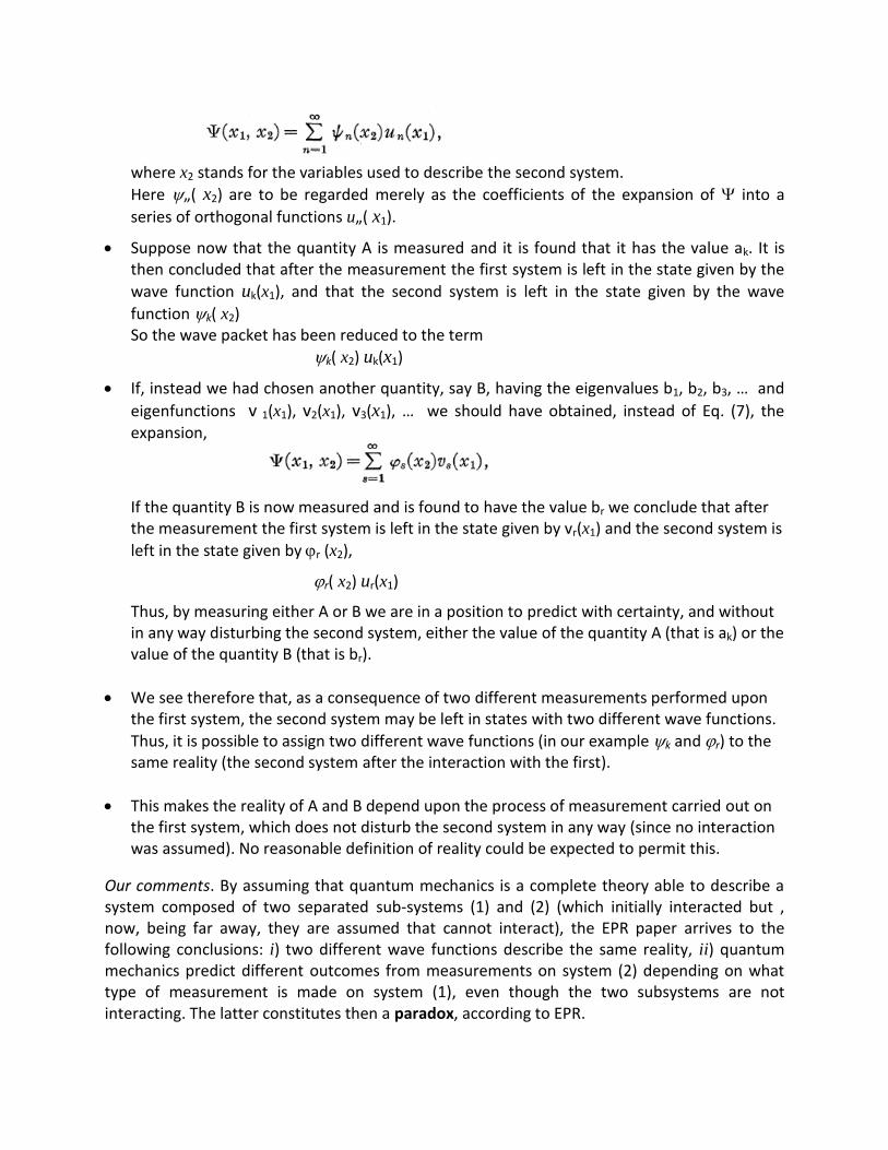
where x2 stands for the variables used to describe the second system.

Here „( x2) are to be regarded merely as the coefficients of the expansion of into a

series of orthogonal functions u„( x1).

Suppose now that the quantity A is measured and it is found that it has the value ak. It is then concluded that after the measurement the first system is left in the state given by the

wave function uk(x1), and that the second system is left in the state given by the wave

function k( x2) So the wave packet has been reduced to the term

k( x2) uk(x1)

If, instead we had chosen another quantity, say B, having the eigenvalues b1, b2, b3, … and

eigenfunctions v 1(x1), v2(x1), v3(x1), … we should have obtained, instead of Eq. (7), the expansion,

If the quantity B is now measured and is found to have the value br we conclude that after the measurement the first system is left in the state given by vr(x1) and the second system is

left in the state given by r (x2),

r( x2) ur(x1)

Thus, by measuring either A or B we are in a position to predict with certainty, and without in any way disturbing the second system, either the value of the quantity A (that is ak) or the value of the quantity B (that is br).

We see therefore that, as a consequence of two different measurements performed upon the first system, the second system may be left in states with two different wave functions.

Thus, it is possible to assign two different wave functions (in our example k and r) to the same reality (the second system after the interaction with the first).

This makes the reality of A and B depend upon the process of measurement carried out on the first system, which does not disturb the second system in any way (since no interaction was assumed). No reasonable definition of reality could be expected to permit this.

Our comments. By assuming that quantum mechanics is a complete theory able to describe a system composed of two separated sub-systems (1) and (2) (which initially interacted but , now, being far away, they are assumed that cannot interact), the EPR paper arrives to the following conclusions: i) two different wave functions describe the same reality, ii) quantum mechanics predict different outcomes from measurements on system (2) depending on what type of measurement is made on system (1), even though the two subsystems are not interacting. The latter constitutes then a paradox, according to EPR.

It is revealing that all the objections of the EPR paper to the quantum theory could be surpassed if the interaction at a distance were accepted. Quantum theory is indeed a non-local theory. On the other hand, that there are different realities associated to a system (i.e. different outcomes from a measurement) is an argument that we have learned to accept as part of quantum behavior.

II.2 The Bohm experimental version to settle the EPR paradox http://plato.stanford.edu/entries/qt-epr/

After fifteen years following the EPR publication, in 1951 David Bohm published a textbook on the quantum theory in which he took a close look at EPR in order to develop a response. Bohm showed how one could mirror the conceptual situation in the EPR thought experiment by looking instead at the dissociation of a diatomic molecule whose total spin angular momentum is (and remains) zero. In the Bohm experiment the atomic fragments separate after interaction, flying off in different directions freely. Subsequently, measurements are made of their spin components (which here take the place of position and momentum), whose measured values would be anti-correlated after dissociation. In the so-called singlet state of the atomic pair (the state after dissociation) if one atom's spin is found to be positive with respect to the orientation of an axis at right angles to its flight path, the other atom would be found to have a negative spin with respect to an axis with the same orientation. Like the operators for position and momentum, spin operators for different orientations do not commute. Moreover, in the experiment outlined by Bohm, the atomic fragments can move far apart from one another and so become appropriate objects for assumptions that restrict the effects of purely local actions. Thus Bohm's experiment mirrors the entangled correlations in EPR for spatially separated systems, allowing for similar arguments and conclusions involving locality, separability, and completeness.

Instead of a diatomic molecule, let’s consider the decay of a neutral pi meson into an electron and a positron (a similar process involving instead the decay of a positronium into two gamma photons is described in more detailed in Section III below).

e-e 0

e

-

e+ 0

Assuming the pion was at rest, the electron and positron travel in opposite direction. The pion has spin zero, hence conservation of angular momentum requires that the electron and positron have opposite spin in the pion’s single state:

2/1 [ )( )( - )( )( ]

If the observer on the left makes a measurement and finds the electron to have spin up (down), the positron must then have spin down (up). That is, the measurements are correlated. This occurs even if the observers are arbitrarily far away.

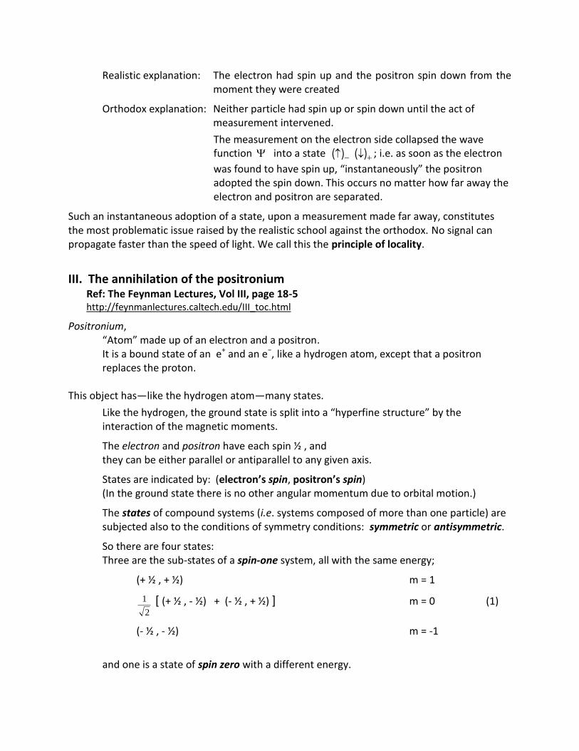
Realistic explanation: The electron had spin up and the positron spin down from the moment they were created

Orthodox explanation: Neither particle had spin up or spin down until the act of measurement intervened.

The measurement on the electron side collapsed the wave function into a state )( )( ; i.e. as soon as the electron

was found to have spin up, “instantaneously” the positron adopted the spin down. This occurs no matter how far away the electron and positron are separated.

Such an instantaneous adoption of a state, upon a measurement made far away, constitutes the most problematic issue raised by the realistic school against the orthodox. No signal can propagate faster than the speed of light. We call this the principle of locality.

III. The annihilation of the positronium Ref: The Feynman Lectures, Vol III, page 18-5 http://feynmanlectures.caltech.edu/III_toc.html

Positronium, “Atom” made up of an electron and a positron. It is a bound state of an e+ and an e−, like a hydrogen atom, except that a positron replaces the proton.

This object has—like the hydrogen atom—many states.

Like the hydrogen, the ground state is split into a “hyperfine structure” by the interaction of the magnetic moments.

The electron and positron have each spin ½ , and they can be either parallel or antiparallel to any given axis.

States are indicated by: (electron’s spin, positron’s spin) (In the ground state there is no other angular momentum due to orbital motion.)

The states of compound systems (i.e. systems composed of more than one particle) are subjected also to the conditions of symmetry conditions: symmetric or antisymmetric.

So there are four states: Three are the sub-states of a spin-one system, all with the same energy;

(+ ½ , + ½) m = 1

2

1 [ (+ ½ , - ½) + (- ½ , + ½) ] m = 0 (1)

(- ½ , - ½) m = -1

and one is a state of spin zero with a different energy.

2

1 [ (+ ½ , - ½) - (- ½ , + ½) ] m = 0 (2)

However, the positronium does not last forever.

The positron is the antiparticle of the electron; they can annihilate each other.

The two particles disappear completely—converting their rest energy into radiation,

which appears as -rays (photons).

In the disintegration, two particles with a finite rest mass go into two or more objects which have zero rest mass.

Case: Disintegration of the spin-zero state of the positronium. It disintegrates into two γ-rays with a lifetime of about 10−10 seconds. The initial and final states are illustrated in Fig. 7 below.

Initial state: we have a positron and an electron close together and with spins antiparallel, making the positronium system.

2

1 [ (+ ½ , - ½) - (- ½ , + ½) ] spin zero state

Final state: After the disintegration there are two photons going out with equal magnitude but opposite momenta,

(because the total momentum after the disintegration must be zero; we are taking the case of the positronium being at rest).

Angular distribution of the outgoing photons

Since the initial state (a) has spin zero, it has no special axis; therefore that state is symmetric under all rotations.

The final state (b) (constituted by photons) must then also be symmetric under all rotations.

That means that all angles for the disintegration are equally likely (3)

The amplitude is the same for a photon to go in any direction.

Of course, once we find one of the photons in some direction the other must be opposite.

Figure 7. Annihilation of positronium and emission of two-photons. We are interested in the polarization state of the outgoing photons.

Polarization of the photons

The only remaining question is about the polarization of the (4) outgoing photons.

In Fig. 7(b), let's call the directions of motion of the two photons the plus and minus Z-axes. See Fig. 8 below.

Photon polarization states: We can use any representations we want for the polarization states of the photons.

We will choose for our description right and left circular polarizations. In the classical theory, right-hand circular polarization has equal components in x and y which are 90∘ out of phase.

Figure 8. Classical picture of the electric field vector.

In the quantum theory, a right-hand circularly (RHC) polarized photon has equal amplitudes to be |x⟩ polarized or |y⟩ polarized, and the amplitudes are 90∘ out of phase. Similarly for left-hand circularly (LHC) polarized photon.

|R ⟩ = 2

1 [ |x⟩ + i |y⟩ ] RHC photon a state

(5)

|L ⟩ = 2

1 [ |x⟩ - i |y⟩ ] LHC photon a state

Case-1: Emitted photons in the RHC states

If the photon going upward is RHC, then angular momentum will be conserved if the downward going photon is also RHC.

Each photon will carry +1 unit of angular momentum with respect to its momentum direction, which means plus and minus one unit about the z-axis.

The total angular momentum will be zero. The angular momentum after the disintegration will be the same as before. See Fig. 9 below.

Fig. 9 Positronium annihilation along the z-axis. The final

state is indicated as |R1R2⟩.

Case-2: Emitted photons in the LHC states There is also the possibility that the two photons go in the LHC state.

Figure 10. Another possibility for positronium annihilation

along the z-axis. The final state is indicated as |L1 L2⟩.

Relationship between the two decay modes mentioned above What is the relation between the amplitudes for these two possible decay modes? The answer comes from using the conservation of parity.

The parity of a state |⟩, relative to a given operator action, is related to whether,

F~ |⟩ = |⟩ even parity or (6) F~ |⟩ = - |⟩ odd parity

Before the decay: Theoretical physicists have shown, in a way that is not easy to explain, that the spin-zero ground state of positronium must be odd. We will just assume that it is odd, and since we will get agreement with experiment, we can take that as sufficient proof.

After the decay: Let's see then what happens if we make an inversion of the process in Fig. 9.

In the QM jargon, we say “let’s apply the operator P~

to the state”.

Here P~

stands for the inversion operator.1

When we apply P~

to the state described in Fig. 9 , the two photons reverse directions and polarizations. The inverted picture looks just like Fig. 10.

Let,

|R1R2⟩ stand for the final state of Fig. 9 (7) in which both photons are RHC,

and

|L1L2⟩ stand for the final state of Fig. 10 (8) in which both photons are LHC.

We notice that an inversion of the photon state in Fig. 9 results in an arrangement equal to the one in Fig. 10; and vice versa. That is,

P~

|R1R2⟩ = |L1L2⟩

(9) P

~|L1L2⟩ = |R1R2⟩

So neither the state |R1R2⟩ nor the state |L1L2⟩ conserve the parity.

So, how to build a state |⟩ such that P~

|⟩ = - |⟩ ?

Answer,

|F ⟩ = | R1 R2⟩ − | L1 L2⟩ (10)

1 An inversion operation means that we should imagine what the system would look like if we were to move each

part of the system to an equivalent point on the opposite side of the origin. When we change x,y,z into −x,−y,−z, all polar vectors (like displacements and velocities) get reversed, but not the axial vectors (like angular momentum—or any vector which is derived from a cross product of two polar vectors). Axial vectors have the same components after an inversion.

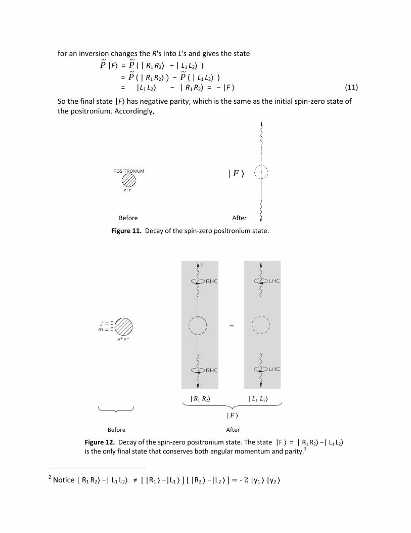
for an inversion changes the R's into L's and gives the state

P~

|F⟩ = P~

( | R1 R2⟩ − | L1 L2⟩ )

= P~

( | R1 R2⟩ ) − P~

( | L1 L2⟩ ) = |L1 L2⟩ − | R1 R2⟩ = − |F ⟩ (11)

So the final state |F⟩ has negative parity, which is the same as the initial spin-zero state of the positronium. Accordingly,

| F ⟩

Before After

Figure 11. Decay of the spin-zero positronium state.

| F ⟩

-

Before After

| R1 R2⟩ | L1 L2⟩

Figure 12. Decay of the spin-zero positronium state. The state |F ⟩ = | R1 R2⟩ −| L1 L2⟩ is the only final state that conserves both angular momentum and parity.2

2 Notice | R1 R2⟩ −| L1 L2⟩ ≠ [ |R1 ⟩ −|L1 ⟩ ] [ |R2 ⟩ −|L2 ⟩ ] = - 2 |y1 ⟩ |y2 ⟩

What does the final state |F ⟩ = | R1 R2⟩ −| L1 L2⟩ mean physically?

First notice that following, ⟨ R1 R2| F ⟩ = 1 and ⟨ L1 L2| F ⟩ = -1.

< R1 R2| F ⟩ = ⟨ R1 R2| [ | R1R2⟩ − | L1 L2⟩ ]

= ⟨ R1 R2| R1 R2⟩ − ⟨ R1 R2| | L1 L2 ⟩

= ⟨ R1| R1 ⟩ ⟨ R2| R2⟩ − ⟨ R1| L1⟩ ⟨ R2| L2⟩

1 . 1 − 0 . 0

⟨ R1 R2| F ⟩ = 1 (12)

Similarly,

⟨ L1 L2| F ⟩ = -1 (13)

The results (12) and (13) mean the following:

If we observe the two photons in two detectors which can be set to count separately the RHC or LHC photons, we will always see two RHC photons together, or two LHC photons together.

That is, if you stand on one side of the positronium and someone else stands on the opposite side, you can measure the polarization (RHC or LHC) and tell the other guy what polarization he will get.

You have a 50-50 chance of catching a RHC photon or a LHC photon; whichever one you get, you can predict that the other will get the same.

Case: What happens if we observe the photon in counters that accept only linearly polarized light?

Let’s assume that it is somewhat easy to measure the polarization of -rays. Suppose that

i) you have a counter that only accepts light with x-polarization,

and

ii) that there is a guy on the other side that also looks for linear polarized light with, say, y-polarization.

What is the chance to pick up the two photons from an annihilation?

What we need to calculate is the amplitude that |F⟩ will be in the state |x1 y2⟩.

Before After

| x1 ⟩

| y2 ⟩

x

y

z

Fig. 13 Experimental set up to observe the output state |x1 y2⟩.

⟨ x1 y2|F ⟩ = ?

⟨ x1 y2|F ⟩ = ⟨ x1 y2| ( | R1 R2⟩ −| L1 L2⟩ )

= ⟨ x1 y2| R1 R2 ⟩ − ⟨ x1 y2| L1 L2 ⟩ (14)

Now although we are working with two-particle amplitudes for the two photons, we can handle them just as we did the single particle amplitudes, since each particle acts independently of the other. That means,

⟨ x1 y2|R1 R2⟩ = ⟨x1|R1⟩ ⟨y2|R2⟩ (15)

Using |R ⟩ = 2

1 [ |x ⟩ + i |y ⟩ ]

|L ⟩ = 2

1 [ |x ⟩ - i |y ⟩ ]

we obtain ⟨ x1 y2| R1 R2⟩ = + i/2

Similarly, we find that ⟨ x1 y2|L1 L2⟩ = − i / 2.

Subtracting these two amplitudes according to (14), we get,

⟨x1 y2|F ⟩ = + i . (16)

So there is a unit probability that if you get a photon in your x-polarized detector, the other guy will get a photon in his y-polarized detector (see Fig. 13).

Case: Now suppose that the other guy sets his counter for x-polarization the same as yours. That is,

i) you have a counter that only accepts light with x-polarization,

and

ii) that there is a guy on the other side that also looks for linear polarized light with x-polarization.

What is the chance to pick up the two photons from an annihilation?

What we are asking is the amplitude that |F⟩ will be in the state |x1 x2⟩.

Answer: He would never get a count when you got one. If you work it through, you will find that,

⟨x1 x2| F ⟩ = 0. (17)

Case: It will, naturally, also work out that if you set your counter for y-polarization, the guy in the other side will get coincident counts only if he is set for x-polarization. Using polarized beam splitters

Now all this leads to an interesting situation. Suppose you were to set up something like a piece of calcite which separates the photons into x -polarized and y -polarized beams

You put a counter in each beam. Let's call one the x -counter and the other the y -counter.

The guy on the other side does the same thing.

The results (16) and (17) above indicate that,

You can always tell him which beam his photon is going to go into.

Whenever you and he get simultaneous counts, you can see which of your detectors caught the photon and then tell him which of his counters had a photon. Let's say that in a certain disintegration you find that a photon went into your x -counter; you can tell him that he must have had a count in his y -counter.

| F ⟩

Before After

| x1 ⟩

| y2 ⟩

| y1 ⟩

| x2⟩

x

y

z

Figure 14. Photon detection with polarized beam splitters at each side.

Now many people who learn quantum mechanics in the usual (old-fashioned) way find this disturbing. They would like to think that,

Once the photons are emitted it goes along as a wave with a definite character.

Since “any given photon” has some “amplitude” to be x-polarized or to be y-polarized,

there should be some chance of picking it up in either the x- or y-counter and that this chance shouldn't depend on what some other person finds out about a completely different photon.

“Someone else making a measurement shouldn't be able to change the probability that I will find something.”

Our quantum mechanics says, however, that,

by making a measurement on photon number one, you can predict precisely what the polarization of photon number two is going to be when it is detected.

This point was never accepted by Einstein, and he worried about it a great deal—it became known as the “Einstein-Podolsky-Rosen paradox.” But when the situation is described as we have done it here, there doesn't seem to be any paradox at all; it comes

out quite naturally that what is measured in one place is correlated with what is measured somewhere else.

The argument that the result is paradoxical runs something like this (let’s enunciate some statements that may be right or wrong, just for the sake of contrasting what quantum mechanics stands):

(1) If you have a counter which tells you whether your photon is RHC or LHC, you can predict exactly what kind of a photon (RHC or LHC) he will find.

(2) The photons he receives must, therefore, each be purely RHC or purely LHC, some of one kind and some of the other.

(3) Surely you cannot alter the physical nature of his photons by changing the kind of observation you make on your photons. No matter what measurements you make on yours, his must still be either RHC or LHC.

(4) Now suppose he changes his apparatus to split his photons into two linearly polarized beams with a piece of calcite so that all of his photons go either into an x-polarized beam or into a y-polarized beam. There is absolutely no way, according to quantum mechanics, to tell into which beam any particular RHC photon will go. There is a 50% probability it will go into the x-beam and a 50% probability it will go into the y-beam. And the same goes for a LHC photon.

(5) Since each photon is RHC or LHC—according to (2) and (3)—each one must have a 50-50 chance of going into the x-beam or the y-beam and there is no way to predict which way it will go.

(6) Yet the theory predicts that if you see your photon go through an x-polarizer you can predict with certainty that his photon will go into his y-polarized beam. This is in contradiction to (5) so there is a paradox.

Nature apparently doesn't see the “paradox,” however, because experiment shows that the prediction in (6) is, in fact, true.

In the argument above, Steps (1), (2), (4), and (6) are all correct, but Step (3), and its consequence (5), are wrong; they are not a true description of nature.

Argument (3) says that by your measurement (seeing a RHC or a LHC photon) you cannot determine which of two alternative events occurs for him (seeing a RHC or a LHC photon), and that even if you do not make your measurement you can still say that his event will occur either by one alternative or the other. But this is not the way Nature works.

Her way requires a description in terms of interfering amplitudes, one amplitude for each alternative.

A measurement of which alternative actually occurs destroys the interference,

but if a measurement is not made you cannot still say that “one alternative or the other is still occurring.”

If you could determine for each one of your photons whether it was RHC and LHC, and also

whether it was x-polarized (all for the same photon) there would indeed be a paradox. But you

cannot do that—it is an example of the uncertainty principle.

Do you still think there is a “paradox”? Make sure that it is, in fact, a paradox about the behavior of Nature, by setting up an imaginary experiment for which the theory of quantum mechanics would predict inconsistent results via two different arguments. Otherwise the “paradox” is only a conflict between reality and your feeling of what reality “ought to be.”

Do you think that it is not a “paradox,” but that it is still very peculiar? On that we can all agree. It is what makes physics fascinating.

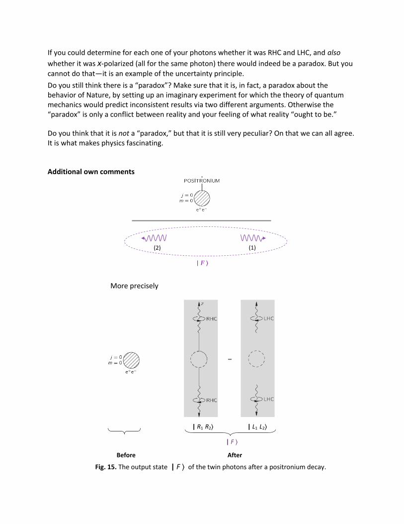
Additional own comments

| x1 ⟩

| y2 ⟩

x y

z

| F ⟩

(2) (1)

More precisely

| F ⟩

-

Before After

| R1 R2⟩ | L1 L2⟩

Fig. 15. The output state | F ⟩ of the twin photons after a positronium decay.

Although the state |F ⟩ is the only one that fulfills the conservation of parity, quantum mechanics allows us to calculate the amplitude probability to obtain another state upon making the system (the two outgoing photons) to interact with some (polarizers) apparatus. For example, we can calculate the amplitude probability ⟨x1 y2|F ⟩ of detecting photon (1) in state | x1 ⟩ and photon (2) in state | y2 ⟩.

| x1 ⟩

| y2 ⟩

x

y

z

| R ⟩

(2)

| x ⟩

| L ⟩ )

(2)

(2)

(1)

(1)

(1)

| y ⟩

| R ⟩

| L ⟩ )

Figure 16. Pictorial representation of the different quantum states

that can be obtained after a measurement. Only three quantum states are indicated (with different color lines) in the figure.

The states shown in Fig. 16 are different possible states after a measurement is performed on the two photons. Notice each possible state is composed of one photon going to one side and another going to the other side. A different color is used in the figure to represent each different entangled state. One state (depicted in green) shows RHC polarization (on the left side) and RHC polarization (on the right side). Another state shows y-polarization (on the photon going left) and x-polarization (on the photon going right). Etc.

If this experiment (the positroniun decay ) is repeated N times, with the

detectors set to detect polarization | S ⟩ on (1) and polarization | T ⟩ on (18) (2) then a fraction |⟨ S1 T2| F ⟩ |2 of N will give such an expected result.

(Correspondingly, similar for any other specific state) The following is not correct: Fig. 16 shows the paths available for a given twin of photons, and that in a particular single experiment all they have to do is to choose one available (19) path.

Indeed, the above cannot be true. We know that the output state of the combined photons is |F ⟩; it is the only one satisfying all the conservation laws in a positronium decay. Fig. 16 shows output states that do not satisfy parity; i.e. they are not (20) allowed outcomes from a decay. Instead, what Fig. 16 shows are states obtained after making a selected measurement.

Statement (20) prevents us from affirming, for example, the following: Once a decay occurs (a single event) a twin of photons can go either path red, or blue or green, each with its own weight of amplitude probabilities. That latter is not true, since each path shown with different colors in Fig. 16 violates the parity conservation. Instead, what occurs is the following: The measurement made on one side forces the state |F ⟩ to collapse on a particular state. The collapsing implies that the other side collapses too (21) in the corresponding twin state. In a single observation (i.e. just one positronium decay), if one of the observers detects the photon in the red state, then he/she can predict with certainty that the observer on the other side will detect the photon on the red state (even though they are far apart in space). This is because the the quantum state is composed of entangled photon. If observer on the right side is set to observe only blue states, the the observer on the left will detect only the corresponding blue state.

IV. BELL’S THEOREM

Determinism of classical mechanics and the imposition of hidden variables in QM Classical mechanics is a deterministic theory. In principle, and particularly when dealing

with just a few particles, we expect to obtain explicitly (after applying Newton’s law) the position and velocity of each participating particle at any time t provided we know their corresponding values at t=0.

It is of course true that in a multiparticles system (like when describing a gas) the motion of the particles can be described only in a statistical manner. This classical indeterminism arises merely from our lack of detailed knowledge about the position and velocities of each molecule at a given time. If we knew those values (although this is practically impossible) classical mechanics conceives, at least in principle, that the motion of each particle could be determined. Maybe such a type of classical indeterminism occurs also in quantum mechanics. That is, quantum mechanics is an incomplete theory maybe because there are other variables, called ‘hidden variables’, of which we are not directly aware, but which are required to determine the system completely. These hidden variables are postulated to behave in a classical deterministic manner. The apparent indeterminism exhibited by a quantum systems arising from our lack of knowledge of the hidden sub-structure of the system. Thus, apparently identical systems are perhaps characterized by different values of one or more hidden variables, which determine in

some way which particular eigenvalues are obtained in a particular measurement.3 In the case of the positronium decay, for example, there might be a classical hidden variable, the value of which was determined when the state |F ⟩ was created and which subsequently determined the experimental results.

However, J. S. Bell in 1965 was able to lay down conditions that all deterministic local theories must satisfy. It turns out those conditions are found to be violated by experiment. Bell suggested,

… 3 B. H. Bransden & C. J. Joachain, Quantum mechanics, Prentice Hall (2000).

http://www.nature.com/news/physics-bell-s-theorem-still-reverberates-1.15435 Before investing too much angst or money, one wants to be sure that Bell correlations really exist. As of now, there are no loophole-free Bell experiments. Experiments in 1982 by a team led by French physicist Alain Aspect2, using well-separated detectors with settings changed just before the photons were detected, suffered from an ‘efficiency loophole’ in that most of the photons were not detected. This allows the experimental correlations to be reproduced by (admittedly, very contrived) local hidden variable theories. In 2013, this loophole was closed in photon-pair experiments using high-efficiency detectors7, 8. But they lacked large separations and fast switching of the settings, opening the ‘separation loophole’: information about the detector setting for one photon could have propagated, at light speed, to the other detector, and affected its outcome. https://www.facebook.com/notes/jon-trevathan/the-einstein-podolsky-and-rosen-epr-paradox-explained/10150198136739263

A preliminary question

A localized region contains a two-particle system< which is known to have a total linear momentum P=0 and total angular momentum L=0.

Suddenly one particle is seen flying to the left and the other to the right. It is verified that the linear momentum is conserved.

If we proceed to measure the angular momentum on the left particle: Once we determine that one particle has spin +1/2 , then we conclude that the other particle has spin – ½. But this conclusion has nothing to do with entanglement, right? No information has travelled instantaneously. The conclusion s based simple on the conservation of angular momentum. Entanglement has to refer to something else.

What would be an example closest to the one expressed above, but with entanglement being involved?

Preliminary answer: First, the example above, except for mentioning the concept of spin, is basically a classical physics example. Avoid mentioning spin and keep talking about angular momentum and the example will be entirely classical physics.

We have, then, to explore the quantum mechanics version of that experiment.

Another preliminary answer: There are different types of entanglements. Two particles can be entangled base on the fact that their total angular momentum must be constant, or that their momentum must be the same, or that their energy must be constant. Answer

Entanglement between two particles has to do with the impossibility to determine, without perturbing the particles, which one carries a specific value of the entangled property. Also, that the particles can have different values of the property; they will adopt a specific value only after the measurement. Notice the latter is not the case for the classical example given above.

Question How can be proved that a particle adopt a value just before the measurement?

(01-2014) Reality depends on the measurement A box contains two balls. One is sent out to the right towards observer A, the other to the left towards observer B. All we know is that, before splitting, they must have had the same color. i) It is one thing to conceptualize that observer-A can report one and only one color

(whatever of three possible colors the ball may have had). Once Observer-A report a color, then we can state what the color of the other ball is.

ii) A different situation is to conceptualize that, before the measurement, the ball can be in any of its three state color; and that upon the measurement the ball acquires a color. Further, to conceptualize that the measurement will influence the color that the ball may acquire.

Question: However, how can we know whether we are facing case i) or case ii)? Answer: From a single event (single measurement) certainly we ca not conclude if we are

facing case i) or ii). To demonstrate we are in case ii) we would have to set up an experiment that

revels the interference that may be inherent in case ii)

Question (01-24-2014) What experiment demonstrates that indeed the two photons have have different

polarization but the polarization-state is adopted right at the moment of detection?

Innsbruck, in 1998, implemented an experiment that allowed fast switch so the measurement could be made right before the measurement (so no possibility that the detector could send a signal to another detector with enough time). But, the latter does not disproved that the photons had already a given polarization.

Question: Does it make sense to talk about the polarization of a single photon? After passing a linear polarizer, indeed we can ascribe a polarization to the passing photon. But when created randomly in a given process, can we ascribe a polarization state to the

photon? Either, a) they have one but we do not know which polarization it is, or b) the photon does not have one, and it acquires one only after the measurement.

Question: If you had to buy detectors without the restriction of being restricted to teaching, which vendor would you choose? Which product?

Nature, Vol 525, pp. 14–15 (03 September 2015)

Quantum ‘spookiness’ passes toughest test yet Experiment plugs loopholes in previous demonstrations of 'action at a distance', against

Einstein's objections — and could make data encryption safer. By Zeeya Merali

John Bell devised a test to show that nature does not 'hide variables' as Einstein had proposed. Physicists have now conducted a virtually unassailable version of Bell's test.