Chapter 11 Analysis of Variance (One-Way) - · PDF fileChapter 11 Analysis of Variance...

Chapter 11

Analysis of Variance(One-Way)

We now develop a statistical procedure for comparing the means of two ormore groups, known as analysis of variance or ANOVA. These groups mightbe the result of an experiment in which organisms are exposed to differenttreatments. Alternately, the groups might be different species or differentage classes of the same species, populations in different locations, or differentgenetic families. The test works by comparing the variance among the groupmeans to the variance of the observations within each group – if the varianceamong group means is large (implying differences in their means) relative tothe variance within groups, the test is significant. This chapter will examinetests for one-way ANOVA, in which a single factor like a treatment affectsthe observations. More complex designs are possible in which several factorsmay influence the observations and may also interact (see Chapter 14 and19).

What do the data look like for a one-way ANOVA design? Suppose weare interested in trapping bark beetles (Coleoptera: Curculionidae: Scolyti-nae) using different chemical baits, which could involve the beetle’s sexpheromones or odors of the trees they colonize. Suppose that three dif-ferent baits (A, B, and C), with a = 3 denoting the number of treatments.The baits are deployed on traps in the forest, with n = 5 replicate traps foreach bait type. A typical experimental design would establish 15 traps in theforest, and then randomly assign a bait to each trap. After a period of time,the traps would be checked and the number of insects caught in each traprecorded (Table 11.1). Because the data are counts, it would not be normally

281

282 CHAPTER 11. ANALYSIS OF VARIANCE (ONE-WAY)

distributed but more likely have a Poisson or negative binomial distribution(see Chapter 5). However, it is often possible to transform count data tohave a distribution closer to the normal by taking the square root or log ofthe counts (see Chapter 15). The third column in Table 11.1 shows the countdata after applying a log transformation. The notation Yij is often used torefer to the observations in ANOVA designs. The i subscript refers to thegroup or treatment, while j is the observation within the treatment. Forexample, Y13 refers to the third observation in the first treatment, which is2.41.

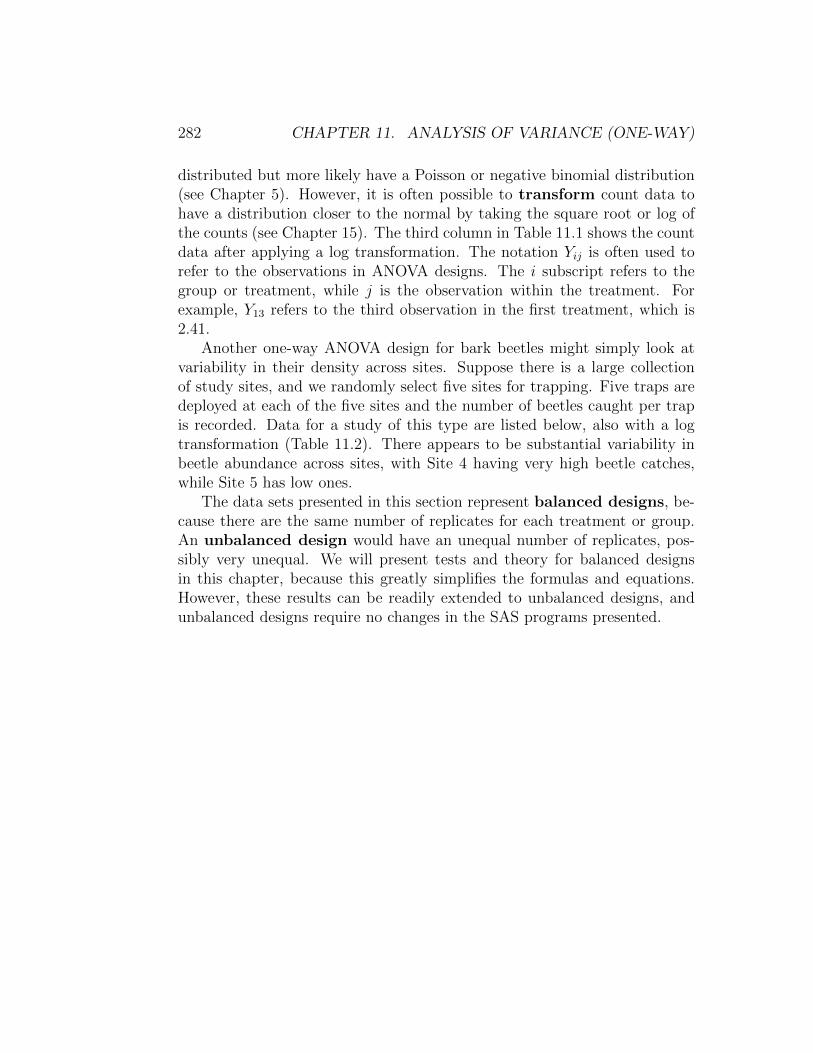
Another one-way ANOVA design for bark beetles might simply look atvariability in their density across sites. Suppose there is a large collectionof study sites, and we randomly select five sites for trapping. Five traps aredeployed at each of the five sites and the number of beetles caught per trapis recorded. Data for a study of this type are listed below, also with a logtransformation (Table 11.2). There appears to be substantial variability inbeetle abundance across sites, with Site 4 having very high beetle catches,while Site 5 has low ones.

The data sets presented in this section represent balanced designs, be-cause there are the same number of replicates for each treatment or group.An unbalanced design would have an unequal number of replicates, pos-sibly very unequal. We will present tests and theory for balanced designsin this chapter, because this greatly simplifies the formulas and equations.However, these results can be readily extended to unbalanced designs, andunbalanced designs require no changes in the SAS programs presented.

283

Table 11.1: Example 1 - Bark beetles captured in a trapping experimentcomparing the attraction to different baits. There were three baits (A, B,and C) and five replicate traps per bait treatment. Also shown are the log-transformed counts (Yij) and subscript values (i, j), and some preliminaryone-way ANOVA calculations.

Treatment Count Yij = i j Yi· (Yij − Yi·)2∑

(Yij − Yi·)2

log10(Count)A 373 2.57 1 1 0.0441A 126 2.10 1 2 0.0676A 255 2.41 1 3 2.3600 0.0025 0.2110A 138 2.14 1 4 0.0484A 379 2.58 1 5 0.0484B 25 1.40 2 1 0.0999B 64 1.81 2 2 0.0088B 62 1.79 2 3 1.7160 0.0055 0.1325B 71 1.85 2 4 0.0180B 54 1.73 2 5 0.0002C 449 2.65 3 1 0.1832C 249 2.40 3 2 0.0317C 69 1.84 3 3 2.2220 0.1459 0.4581C 199 2.30 3 4 0.0061C 84 1.92 3 5 0.0912


Table 11.2: Example 2 - Bark beetles captured in a trapping study comparingtheir abundance at five randomly chosen study sites. There were five replicatetraps per site. Also shown are the log-transformed counts (Yij) and subscriptvalues (i, j), and some preliminary one-way ANOVA calculations.

Site Count Yij = i j Yi· (Yij − Yi·)2∑

(Yij − Yi·)2

log10(Count)1 137 2.14 1 1 0.01641 101 2.00 1 2 0.00011 113 2.05 1 3 2.0120 0.0014 0.15981 48 1.68 1 4 0.11021 155 2.19 1 5 0.03172 156 2.19 2 1 0.07842 165 2.22 2 2 0.06252 652 2.81 2 3 2.4700 0.1156 0.47302 179 2.25 2 4 0.04842 757 2.88 2 5 0.16813 278 2.44 3 1 0.03763 197 2.29 3 2 0.00193 95 1.98 3 3 2.2460 0.0708 0.34193 395 2.60 3 4 0.12533 83 1.92 3 5 0.10634 2540 3.40 4 1 0.49564 613 2.79 4 2 0.00884 200 2.30 4 3 2.6960 0.1568 0.76004 251 2.40 4 4 0.08764 390 2.59 4 5 0.01125 18 1.26 5 1 0.00445 16 1.20 5 2 0.00005 11 1.04 5 3 1.1940 0.0237 0.04595 21 1.32 5 4 0.01595 14 1.15 5 5 0.0019

11.1. ANOVA MODELS 285

11.1 ANOVA models

We now examine the statistical models that are used in one-way ANOVA.There are two models for one-way ANOVA, known as fixed or random effectsmodels, but sometimes called Model I and II. This classification is based onhow the groups in the design are defined or generated. We begin by definingfixed and random effects, then present the statistical models and hypothesesfor each type.

11.1.1 Fixed and random effects

For groups generated by different treatments in an experiment, or purposelychosen groups of organisms such as different species, sexes, or ages, the groupsare classified as fixed effects. They are called fixed effects because thesegroups are the only ones of interest to the investigator, and the only oneson which a statistical inference can be made (Littell et al. 1996, McCullochand Searle 2001). They are also incorporated in statistical models as fixedparameters. Groups that are generated by a process of random sampling areclassified as a random effects (Littell et al. 1996, McCulloch and Searle2001). For example, suppose we want to examine the fish populations in alarge number of lakes, and are interested in how body length varies acrosslakes. If we randomly sample the lakes to be examined, from a large col-lection of lakes, then lake would be classified as a random effect. In manygenetic experiments, families are chosen at random from a larger collection offamilies, making family a random effect. Random effects are incorporated instatistical models as random variables, typically with a normal distribution.

These definitions suggest a simple test for fixed vs. random effects – if thegroups are a random sample from a large collection you have a random effect,otherwise a fixed effect. Although it is usually possible to declare an effectas either fixed or random, in practice it is sometimes difficult to decide. Forexample, suppose that a particular organism occurs at only a small numberof locations. If we randomly select a subset of these locations to sample,seemingly implying a random effect, the overall number of locations is stillfinite. In this scenario, location may be better classified as a fixed effect.


11.1.2 Fixed effects model

Suppose that we want to model the observations in the bark beetle trap-ping experiment, Example 1, where different baits are used. Recall that thesymbol Yij stand for the jth observation in the ith treatment group, wherei = 1, 2, 3 and j = 1, 2, 3, 4, 5. For example, Y11 = 2.57 and Y12 = 2.10, whileY32 = 2.40 (see Table 11.1). One commonly used model for such a design is

Yij = µ+ αi + εij (11.1)

where µ is a parameter setting the grand mean (the overall mean) of theobservations, αi is the deviation from the grand mean caused by the ithtreatment (McCulloch and Searle 2001), and εij ∼ N(0, σ2). It is usuallyassumed that

∑αi = 0, i.e., the treatment effect terms sum to zero. The εij

term represents random departures from the mean value for the ith treat-ment, due to natural variability among the observations. The εij values arealso assumed to be independent (Chapter 4). In practice, these parameterswould be unknown but could be estimated from the data. The same modelcan be used to describe the observations for experiments with any numberof treatments (any a value) as well as replicates per treatments (any n),as well as experiments where the number of observations is unequal amongtreatments.

It follows that for the ith treatment, E[Yij] = µ + αi and V ar[Yij] = σ2,using the rules for expected values and variances. Thus, for the ith treatmentwe have Yij ∼ N(µ+ αi, σ

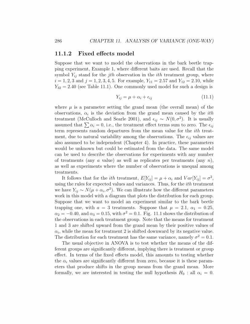
2). We can illustrate how the different parameterswork in this model with a diagram that plots the distribution for each group.Suppose that we want to model an experiment similar to the bark beetletrapping one, with a = 3 treatments. Suppose that µ = 2.1, α1 = 0.25,α2 = −0.40, and α3 = 0.15, with σ2 = 0.1. Fig. 11.1 shows the distribution ofthe observations in each treatment group. Note that the means for treatment1 and 3 are shifted upward from the grand mean by their positive values ofαi, while the mean for treatment 2 is shifted downward by its negative value.The distribution for each treatment has the same variance, namely σ2 = 0.1.

The usual objective in ANOVA is to test whether the means of the dif-ferent groups are significantly different, implying there is treatment or groupeffect. In terms of the fixed effects model, this amounts to testing whetherthe αi values are significantly different from zero, because it is these param-eters that produce shifts in the group means from the grand mean. Moreformally, we are interested in testing the null hypothesis H0 : all αi = 0.


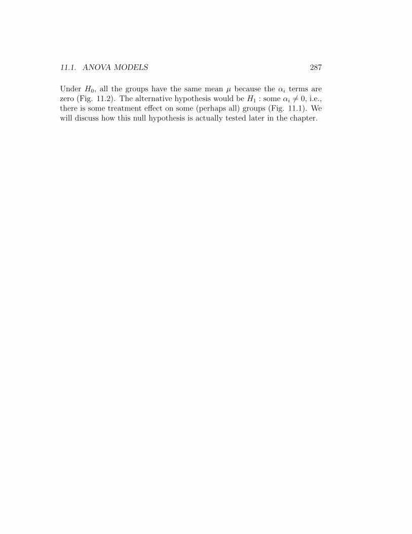
Under H0, all the groups have the same mean µ because the αi terms arezero (Fig. 11.2). The alternative hypothesis would be H1 : some αi 6= 0, i.e.,there is some treatment effect on some (perhaps all) groups (Fig. 11.1). Wewill discuss how this null hypothesis is actually tested later in the chapter.


Figure 11.1: Fixed effects model for one-way ANOVA, under H1 : someαi 6= 0.

Figure 11.2: Fixed effects model for one-way ANOVA, under H0 : all αi = 0.


11.1.3 Random effects model

Suppose that we now want to model the variability in bark beetle abundanceacross different sites, such as in the Example 2 study. Let Yij stand for the jthobservation at the ith sampled site, with i = 1, 2, 3, 4, 5 and j = 1, 2, 3, 4, 5.We have Y11 = 4.92, Y12 = 4.62, and so forth (see Table 11.2). A commonstatistical model for this design is

Yij = µ+ Ai + εij (11.2)

where µ is again a parameter setting the grand mean (the overall mean) ofthe observations, with Ai a random deviation from the grand mean due to theith site (McCulloch and Searle 2001), and εij ∼ N(0, σ2). It is assumed thatAi is normally distributed with mean zero and variance σ2

A, or Ai ∼ N(0, σ2A).

Note that in the random effects model the group effect is indeed a randomvariable, one whose variance is unknown but can be estimated from the data.The variances σ2

A and σ2 are collectively called the variance componentsof the model.

For the ith group sampled, it can be shown that E[Yij] = µ + Ai andV ar[Yij] = σ2, using the rules for expected values and variances. Thus, forthe ith treatment we have Yij ∼ N(µ + Ai, σ

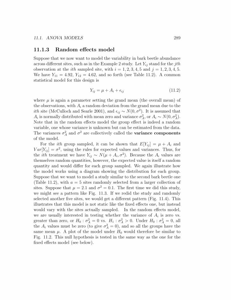
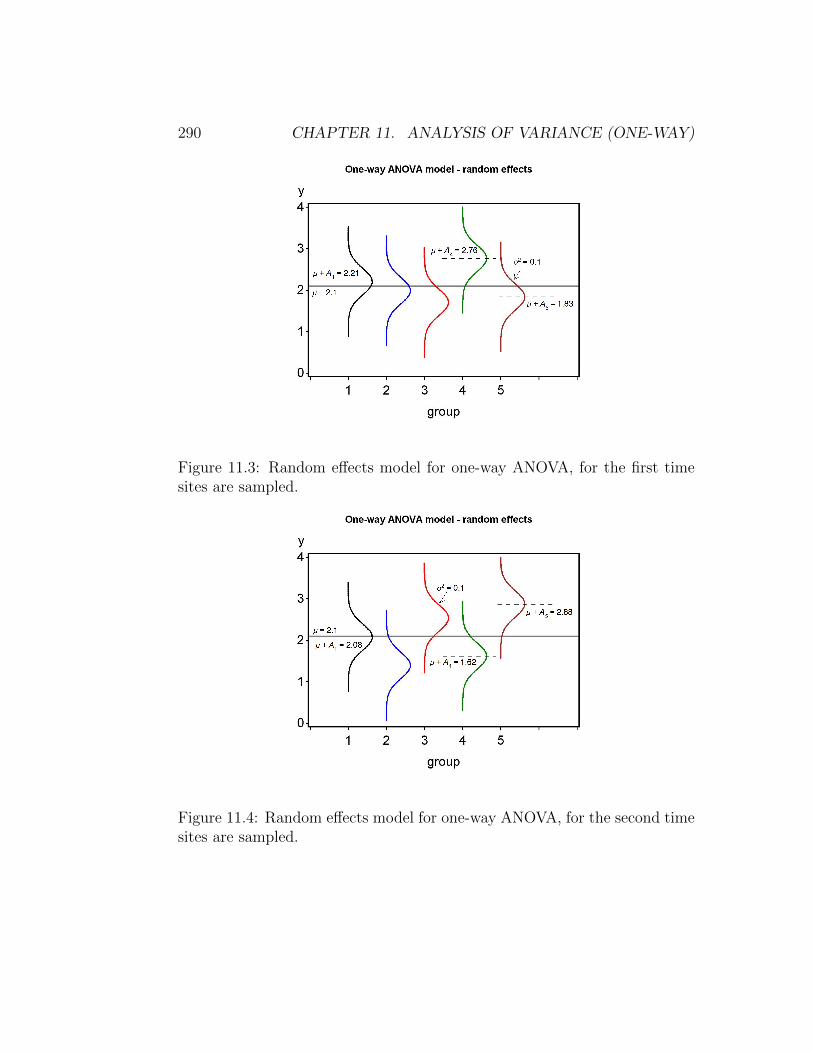
2). Because the Ai values arethemselves random quantities, however, the expected value is itself a randomquantity and would differ for each group sampled. We again illustrate howthe model works using a diagram showing the distribution for each group.Suppose that we want to model a study similar to the second bark beetle one(Table 11.2), with a = 5 sites randomly selected from a larger collection ofsites. Suppose that µ = 2.1 and σ2 = 0.1. The first time we did this study,we might see a pattern like Fig. 11.3. If we redid the study and randomlyselected another five sites, we would get a different pattern (Fig. 11.4). Thisillustrates that this model is not static like the fixed effects one, but insteadwould vary with the sites actually sampled. In the random effects model,we are usually interested in testing whether the variance of Ai is zero vs.greater than zero, or H0 : σ2

A = 0 vs. H1 : σ2A > 0. Under H0 : σ2

A = 0, allthe Ai values must be zero (to give σ2

A = 0), and so all the groups have thesame mean µ. A plot of the model under H0 would therefore be similar toFig. 11.2. This null hypothesis is tested in the same way as the one for thefixed effects model (see below).


Figure 11.3: Random effects model for one-way ANOVA, for the first timesites are sampled.

Figure 11.4: Random effects model for one-way ANOVA, for the second timesites are sampled.

11.2. HYPOTHESIS TESTING FOR ANOVA 291

11.2 Hypothesis testing for ANOVA

We now develop a statistical test for the null hypotheses in both fixed andrandom effects models, either H0 : all αi = 0 or H0 : σ2

A = 0. We will firstpresent the test and explain how it works in terms of different estimates ofthe variance, then later show it is another example of a likelihood ratio test.

11.2.1 Sums of squares and mean squares

Suppose the data are described by a fixed effects model, for which the hy-potheses are H0 : all αi = 0 vs. H1 : some αi 6= 0. It is clear that if H1 istrue, then the observations for the different groups will be shifted from thegrand mean, as shown in Fig. 11.1, and in particular Yij ∼ N(µ + αi, σ

2)for each group. For a random effects model, we have H0 : σ2

A = 0 vs.H1 : σ2

A > 0. If H1 is true, we would also expected the observations for thedifferent groups to be shifted away from the grand mean (Fig. 11.3), andin particular Yij ∼ N(µ + Ai, σ

2). How can we estimate this shift in actualdata? How large must this shift be to be judged statistically significant?

We begin by calculating the means for each group using the data. Theseare labeled as Yi· and are called group means. The ‘·’ subscript implies themean was calculated using all the observations in that group (j = 1, 2, . . . , n).We then calculate the mean of the group means, called the grand mean andlabeled as ¯Y . If the ith group is shifted from the grand mean, we can measurethis shift using the quantity Yi· − ¯Y . In fact, this quantity estimates αi forthe ith group, and so is a direct measure of any group effect (see section onmaximum likelihood estimation below). If these quantities are small then thissuggests H0 might be true, whereas if they are large this provides evidence forH1. We can obtain a single measure of these shifts by squaring and summingthem across all groups, to obtain a quantity called the sum of squares amonggroups or SSamong, because it measures variation in the observations amonggroups:

SSamong = n

a∑i=1

(Yi· − ¯Y )2. (11.3)

Note the sample size n in this expression, which we will justify below. Tomake this quantity more concrete, we will calculate SSamong for Example 1,the bark beetle trapping experiment. We first calculate the sample mean for


each group for the log-transformed data, as shown in Table 11.1. Then, thegrand mean is estimated using the mean of these means, or

¯Y =

∑ai=1 Yi·a

=2.3600 + 1.7160 + 2.2220

3=

6.2980

3= 2.0993. (11.4)

We then have

SSamong = n

a∑j=1

(Yi· − ¯Y )2 (11.5)

= 5[(2.3600− 2.0993)2 + (1.7160− 2.0993)2 + (2.2220− 2.0993)2

](11.6)

= 5 [0.0680 + 0.1469 + 0.0151] (11.7)

= 1.1500 (11.8)

SSamong has a−1 degrees of freedom, where a is the number of groups. There

are a − 1 degrees of freedom because there are a terms of the form Yi· − ¯Yin the sum of squares, but these sum to zero so there are really only a − 1independent terms (similar to the n − 1 degrees of freedom for the samplevariance s2). The next step is to convert SSamong to a sample variance,dividing it by a− 1. This quantity is called the mean square among groups:

MSamong =SSamonga− 1

=n∑a

j=1(Yi· − ¯Y )2

a− 1. (11.9)

For the bark beetle experiment, we find that


=1.1500

3− 1= 0.5750. (11.10)

So, what variance does MSamong estimate? If H0 is true and there are nogroup effects, we would expect Yi· to have a variance of σ2/n, because it isa sample mean composed of n observations in the ith group (which have avariance of σ2). MSamong estimates this variance multiplied by n, becauseof the n term in numerator, and so actually estimates nσ2/n = σ2. On theother hand, if H1 is true then there are group effects, and we would expect thegroup means to be shifted away from the grand mean. This should increasethe size of MSamong. Thus, MSamong estimates σ2 if H0 is true butbecomes larger if H1 is true.


Expected values provide another way to understand how group effectsinfluence MSamong. For the fixed effects model, we have

E[MSamong] =n∑α2i

a− 1+ σ2, (11.11)

while

E[MSamong] = nσ2A + σ2. (11.12)

for the random effects model (Winer et al. 1991). Note how E[MSamong]increases as the group effects increase, above a baseline level setby σ2. For the fixed effects model, larger groups effects would involve largervalues of αi, while for the random effects model a larger value of σ2

A.

We next develop an estimate of the variance σ2 that is free of any group ef-fects. This variance estimate is based on a quantity called the sum of squareswithin groups or SSwithin, because it measures variation of the observationswithin each group. It is defined by the formula

SSwithin =a∑i=1

n∑j=1

(Yij − Yi·)2 (11.13)

=n∑j=1

(Y1j − Y1·)2 + . . .+

n∑j=1

(Yaj − Ya·)2. (11.14)

It has a(n− 1) degrees of freedom, because there are a sum of squares termseach with n − 1 degrees of freedom. We can obtain an estimate of σ2 bydividing this sum of squares by its degrees of freedom, to obtain the meansquare within groups:

MSwithin =SSwithina(n− 1)

=

∑ai=1

∑nj=1(Yij − Yi·)2

a(n− 1). (11.15)

This quantity estimates σ2 because it simply averages estimates of σ2 for


each group. With some rearrangement, we can write MSwithin as

MSwithin =

∑ai=1


a(n− 1)(11.16)

=

∑(Y1j − Y1·)

2 + . . .+∑

(Yaj − Ya·)2

a(n− 1)(11.17)

=

∑(Y1j−Y1·)2n−1

+ . . .+∑

(Yaj−Ya·)2n−1

a(11.18)

=s2

1 + . . .+ s2a

a. (11.19)

Each term in the numerator of this expression is the sample variance s2

for each group, which is then averaged across all groups to yield an overallor pooled estimate of σ2. The word ‘pooled’ in statistics often indicates acombined estimate of a variance. It can also be shown that E[MSwithin] = σ2,regardless of any group effects.

We now calculate MSwithin for the bark beetle experiment. We first needto calculate the quantity (Yij − Yi·)2 for the observations in each group andthen sum these for each group (see Table 11.1). Summing these quantitiesin turn across all groups, we obtain

SSwithin = 0.2110 + 0.1325 + 0.4581 = 0.8016. (11.20)

(11.21)

We then have


=0.8016

3(5− 1)= 0.0668. (11.22)

(11.23)

There is one more sum of squares that can be calculated in one-wayANOVA, the total sum of squares. It is defined as

SStotal =a∑i=1

n∑j=1

(Yij − ¯Y )2. (11.24)

It measures the variability of the observations around the grand mean of thedata ( ¯Y ) and has an − 1 degrees of freedom. Applying this formula to theExample 1 data set, we obtain SStotal = 1.9516 after much calculation.


An interesting feature of the sum of squares is that they add to the totalsum of squares, as do the degrees of freedom. In particular, we have

SSamong + SSwithin = SStotal (11.25)

and

(a− 1) + a(n− 1) = an− 1. (11.26)

Thus, the sum of squares and degrees of freedom can be neatly partitionedinto components corresponding to among group and within group variation.We will illustrate this relationship further in the section below on ANOVAtables.

11.2.2 F statistic and distribution

We next describe the statistic used to test H0 : all αi = 0 for the fixed effectmodel, and H0 : σ2

A = 0 for the random effects one. It is simply the ratio ofMSamong and MSwithin, or

Fs =MSamongMSwithin

. (11.27)

If H0 is true for either model, both MSamong and MSwithin estimate σ2 andwe would expect their ratio, Fs, to be small and on the order of one. However,if H0 is false and H1 is true, we would expect MSamong to become larger andFs to increase. We would therefore reject H0 for large values of Fs.

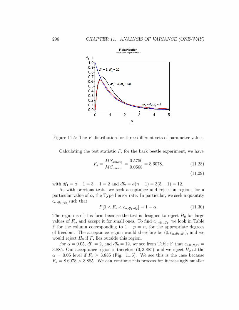
To complete our testing procedure and find P values, we need to know thedistribution of Fs under H0. It turns out this statistic has an F distributionunder H0, whose shape and location is governed by two parameters, the de-grees of freedom for MSamong and MSwithin. These are called the numeratorand denominator degrees of freedom, which we abbreviate as df1 and df2. Inparticular, for one-way ANOVA we have df1 = a − 1 and df2 = a(n − 1).Figure 11.5 shows the F distribution for three different sets of parametervalues. Note that distribution can have a maximum at y = 0 for small valuesof df1, while larger values of df2 decrease the probability in the right tail ofthe distribution.

Table F gives the quantiles of the F distribution for different values of thedegrees of freedom and the cumulative probability p. Statistical tests thatmake use of the F distribution are typically called F tests.


Figure 11.5: The F distribution for three different sets of parameter values

Calculating the test statistic Fs for the bark beetle experiment, we have

Fs =MSamongMSwithin

=0.5750

0.0668= 8.6078, (11.28)

(11.29)

with df1 = a− 1 = 3− 1 = 2 and df2 = a(n− 1) = 3(5− 1) = 12.As with previous tests, we seek acceptance and rejection regions for a

particular value of α, the Type I error rate. In particular, we seek a quantitycα,df1,df2 such that

P [0 < Fs < cα,df1,df2 ] = 1− α. (11.30)

The region is of this form because the test is designed to reject H0 for largevalues of Fs, and accept it for small ones. To find cα,df1,df2 , we look in TableF for the column corresponding to 1 − p = α, for the appropriate degreesof freedom. The acceptance region would therefore be (0, cα,df1,df2), and wewould reject H0 if Fs lies outside this region.

For α = 0.05, df1 = 2, and df2 = 12, we see from Table F that c0.05,2,12 =3.885. Our acceptance region is therefore (0, 3.885), and we reject H0 at theα = 0.05 level if Fs ≥ 3.885 (Fig. 11.6). We see this is the case becauseFs = 8.6078 > 3.885. We can continue this process for increasingly smaller


α and eventually find that for α = 0.005 we can still reject H0, but not forα = 0.001. We therefore have P < 0.005 for this test, because α = 0.005is the smallest value of α for which we can reject H0 (see Chapter 10). AnF test in ANOVA would often be reported as follows: ‘There was a highlysignificant difference among the different baits in the number of bark beetlestrapped (F2,12 = 8.6078, P < 0.005).’ Note that the degrees of freedom aregiven as subscripts.

Figure 11.6: Acceptance and rejection regions for α = 0.05

11.2.3 ANOVA tables

We can organize the different sum of squares and mean squares into anANOVA table. It lists the different sources of variation in the data (among,within, and total), their degrees of freedom, sums of squares and meansquares, and then the F statistic and its P value. Table 11.3 shows thegeneral layout of such a table for one-way ANOVA designs, while Table 11.4gives the results for the Example 1 analysis. Note the additive relationshipfor the degrees of freedom and sum of squares.

298CHAPTER

11.ANALYSIS

OFVARIA

NCE(O

NE-W

AY)

Table 11.3: General ANOVA table for one-way designs with a groups and n observations per group, showingformulas for different mean squares and the F test.

Source df Sum of squares Mean square FsAmong a− 1 SSamong = n

∑ai=1(Yi· − ¯Y )2 MSamong = SSamong/(a− 1) MSamong/MSwithin

Within a(n− 1) SSwithin =∑a

i=1

∑nj=1(Yij − Yi·)2 MSwithin = SSwithin/a(n− 1)

Total an− 1 SStotal =∑a

i=1

∑nj=1(Yij − ¯Y )2

Table 11.4: ANOVA table for the Example 1 data set, including a P value for the test.

Source df Sum of squares Mean square Fs PAmong 2 1.1500 0.5750 8.6078 < 0.005Within 12 0.8016 0.0668Total 14 1.9516


11.2.4 One-way ANOVA for Example 1 - SAS demo

The same calculations for the bark beetle experiment can be carried out inSAS using proc glm (SAS Institute Inc. 2014a). This procedure is primarilyintended for fixed effects ANOVA models, with proc mixedthe best choice forrandom effects models. However, the F test would be the same in eitherprocedure.

The SAS program for one-way ANOVA is a bit more complicated thanprevious programs, so we will examine it a section at a time. The first stepis to read in the observations using a data step, with one variable denotingthe treatment (treat) and a second the number of beetles captured (count).As discussed earlier, it is common to log-transform count data, and so wegenerate a variable y that is the log 10 (log base 10) of count. The data stepis followed by a print statement to print the data set. See section below.

* bark_beetle_experiment.sas;

options pageno=1 linesize=80;

goptions reset=all;

title "One-way ANOVA for bark beetle trapping experiment";

data bark_beetle;

input treat $ count;

* Apply transformations here;

y = log10(count);

datalines;

A 373

A 126

A 255

etc.

C 199

C 84

;

run;

* Print data set;

proc print data=bark_beetle;

run;

We next plot the data using the SAS procedure gplot (SAS Institute Inc.2014b). The basic idea is to plot, for each treatment group, the individualdata points along with their mean (Y ) ± one standard error (s/

√n). The

plot statement tells gplot to plot the variable y on the y-axis and treat onthe x-axis of the plot. The appearance of the points is controlled by the


symbol1 statement, which among other things specifies that the points beplotted along with their means ± one standard error, with the means joinedby a line, using the option i=std1mjt. Other options in the symbol statementcontrol the type and size of the points, and line width. The vaxis=axis1 andhaxis=axis1 options control the visual appearance of the x- and y-axes. Seebelow.

* Plot means, standard errors, and observations;

proc gplot data=bark_beetle;

plot y*treat=1 / vaxis=axis1 haxis=axis1;

symbol1 i=std1mjt v=star height=2 width=3;

axis1 label=(height=2) value=(height=2) width=3 major=(width=2) minor=none;

run;

The next section of the program conducts the one-way ANOVA and F testusing proc glm. The class statement tells SAS that the variable treat is theone that defines different groups in the ANOVA (see listing below). Themodel statement basically tells SAS the form of the ANOVA model. Recallthat the model for fixed effects one-way ANOVA is given by the equation

Yij = µ+ αi + εij. (11.31)

If we equate Yij with y, and αi with treat, we see there are similarities betweenthe fixed effects model and the SAS model statement. In fact, SAS assumesyou want a grand mean µ unless otherwise specified, as well as the error termεij. As we examine more complex ANOVA models in later chapters, we willsee there is nearly a one-to-one correspondence between these models andthe corresponding SAS model statement.

* One-way ANOVA with all fixed effects;

proc glm data=bark_beetle;

class treat;

model y = treat;

* Calculate means for each group;

means treat;

output out=resids p=pred r=resid;

run;

The means statement causes glm to calculate means for each treat group.The other statements generate graphs that are used to examine some of theassumptions of ANOVA – we will defer their discussion to later chapters.

The complete SAS program and output are listed below. The outputshows the same F test in three different locations within the proc glm output.


The first is in a format resembling an ANOVA table, and then two other timescorresponding to Type I and III sums of squares. These are different ways ofcalculating the sums of squares and tests, with Type III sums of squares moregenerally useful for ANOVA designs. For one-way ANOVA the results are thesame, and we see that there was a highly significant difference among groups(F2,12 = 8.60, P = 0.0048). Inspection of the graph and means suggests thattreatment A caught the most beetles, followed by C and then B.

SAS Program

* bark_beetle_experiment.sas;


goptions reset=all;

title "One-way ANOVA for bark beetle trapping experiment";

data bark_beetle;



y = log10(count);

datalines;

A 373

A 126

A 255

A 138

A 379

B 25

B 64

B 62

B 71

B 54

C 449

C 249

C 69

C 199

C 84

;

run;

* Print data set;


run;






run;


* One-way ANOVA with all fixed effects;

proc glm data=bark_beetle;

class treat;

model y = treat;

* Calculate means for each group;

means treat;

output out=resids p=pred r=resid;

run;

goptions reset=all;

title "Diagnostic plots to check ANOVA assumptions";

* Plot residuals vs. predicted values;

proc gplot data=resids;

plot resid*pred=1 / vaxis=axis1 haxis=axis1;

symbol1 v=star height=2 width=3;


run;

* Normal quantile plot of residuals;

proc univariate noprint data=resids;

qqplot resid / normal waxis=3 height=4;

run;

quit;


SAS Output

One-way ANOVA for bark beetle trapping experiment 1

09:32 Tuesday, August 31, 2010

Obs treat count y

1 A 373 2.57171

2 A 126 2.10037

3 A 255 2.40654

4 A 138 2.13988

5 A 379 2.57864

6 B 25 1.39794

7 B 64 1.80618

8 B 62 1.79239

9 B 71 1.85126

10 B 54 1.73239

11 C 449 2.65225

12 C 249 2.39620

13 C 69 1.83885

14 C 199 2.29885

15 C 84 1.92428



The GLM Procedure

Class Level Information

Class Levels Values

treat 3 A B C

Number of Observations Read 15

Number of Observations Used 15



The GLM Procedure


Dependent Variable: y

Sum of

Source DF Squares Mean Square F Value Pr > F

Model 2 1.14818176 0.57409088 8.60 0.0048

Error 12 0.80114853 0.06676238

Corrected Total 14 1.94933029

R-Square Coeff Var Root MSE y Mean

0.589013 12.30880 0.258384 2.099182

Source DF Type I SS Mean Square F Value Pr > F

treat 2 1.14818176 0.57409088 8.60 0.0048

Source DF Type III SS Mean Square F Value Pr > F

treat 2 1.14818176 0.57409088 8.60 0.0048



The GLM Procedure

Level of --------------y--------------

treat N Mean Std Dev

A 5 2.35942757 0.22948244

B 5 1.71603276 0.18282085

C 5 2.22208543 0.33793710


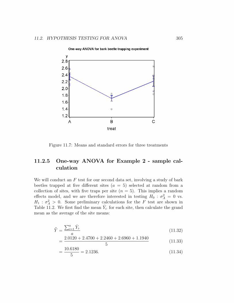
Figure 11.7: Means and standard errors for three treatments

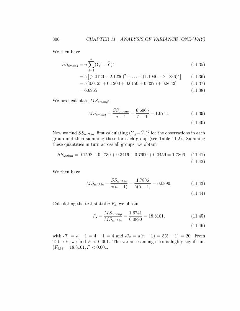
11.2.5 One-way ANOVA for Example 2 - sample cal-culation

We will conduct an F test for our second data set, involving a study of barkbeetles trapped at five different sites (a = 5) selected at random from acollection of sites, with five traps per site (n = 5). This implies a randomeffects model, and we are therefore interested in testing H0 : σ2

A = 0 vs.H1 : σ2

A > 0. Some preliminary calculations for the F test are shown inTable 11.2. We first find the mean Yi· for each site, then calculate the grandmean as the average of the site means:

¯Y =

∑ai=1 Yi·a

(11.32)

=2.0120 + 2.4700 + 2.2460 + 2.6960 + 1.1940

5(11.33)

=10.6180

5= 2.1236. (11.34)


We then have

SSamong = n

a∑j=1

(Yi· − ¯Y )2 (11.35)

= 5[(2.0120− 2.1236)2 + . . .+ (1.1940− 2.1236)2

](11.36)

= 5 [0.0125 + 0.1200 + 0.0150 + 0.3276 + 0.8642] (11.37)

= 6.6965 (11.38)

We next calculate MSamong:


=6.6965

5− 1= 1.6741. (11.39)

(11.40)

Now we find SSwithin, first calculating (Yij− Yi·)2 for the observations in eachgroup and then summing these for each group (see Table 11.2). Summingthese quantities in turn across all groups, we obtain

SSwithin = 0.1598 + 0.4730 + 0.3419 + 0.7600 + 0.0459 = 1.7806. (11.41)

(11.42)

We then have


=1.7806

5(5− 1)= 0.0890. (11.43)

(11.44)

Calculating the test statistic Fs, we obtain

Fs =MSamongMSwithin

=1.6741

0.0890= 18.8101, (11.45)

(11.46)

with df1 = a − 1 = 4 − 1 = 4 and df2 = a(n − 1) = 5(5 − 1) = 20. FromTable F, we find P < 0.001. The variance among sites is highly significant(F4,12 = 18.8101, P < 0.001.


11.2.6 One-way ANOVA for Example 2 - SAS demo

We can carry out the F test as well as estimate the variance components(σ2

A and σ2) for the random effects model using SAS. The first section of theprogram involving the data step and gplot graph is similar to the fixed effectsprogram. The next section of the program fits the random effects model tothe data and conducts the F test, using proc mixed (see listing below). Asbefore, the class statement tells SAS that the variable site is the one thatdefines different groups in the ANOVA. Now recall that the model for randomeffects one-way ANOVA is given by the equation

Yij = µ+ Ai + εij. (11.47)

Note that Ai corresponds to site in the bark beetle study. In proc mixed,fixed effects in the model are placed in a model statement, while any randomeffects are listed in a random statement (SAS Institute Inc. 2014a). Becauseour random effects model only has one random effect, site, this is listed inthe random statement. There are no fixed effects in this model, so the model

statement lists nothing after the equals sign. The option ddfm=kr specifies ageneral method of calculating the degrees of freedom that works well undermany circumstances, including more complicated models.

* One-way ANOVA with random effects - F test;

proc mixed method=type3 data=bark_beetle;

class site;

model y = / ddfm=kr;

random site;

run;

* One-way ANOVA with random effects - variance components;

proc mixed cl data=bark_beetle;

class site;

model y = / ddfm=kr outp=resids;

random site;

run;

Why is proc mixed invoked twice in this program? The first one generatesthe F statistic for testing H0 : σ2

A = 0 vs. H1 : σ2A > 0, using the option

method=type3. This is not the default in proc mixed, which appears moredesigned to estimate the variance components in random effects (Littell etal. 1996). If we drop this option, as in the second proc mixed statement, we


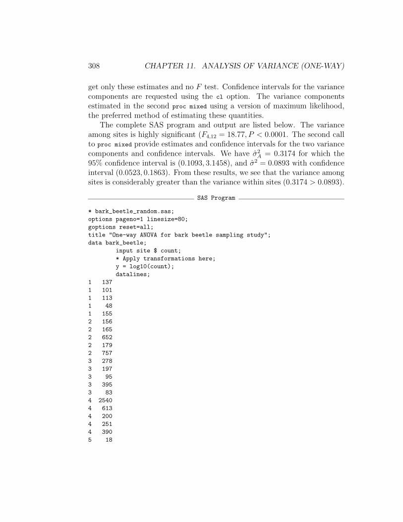
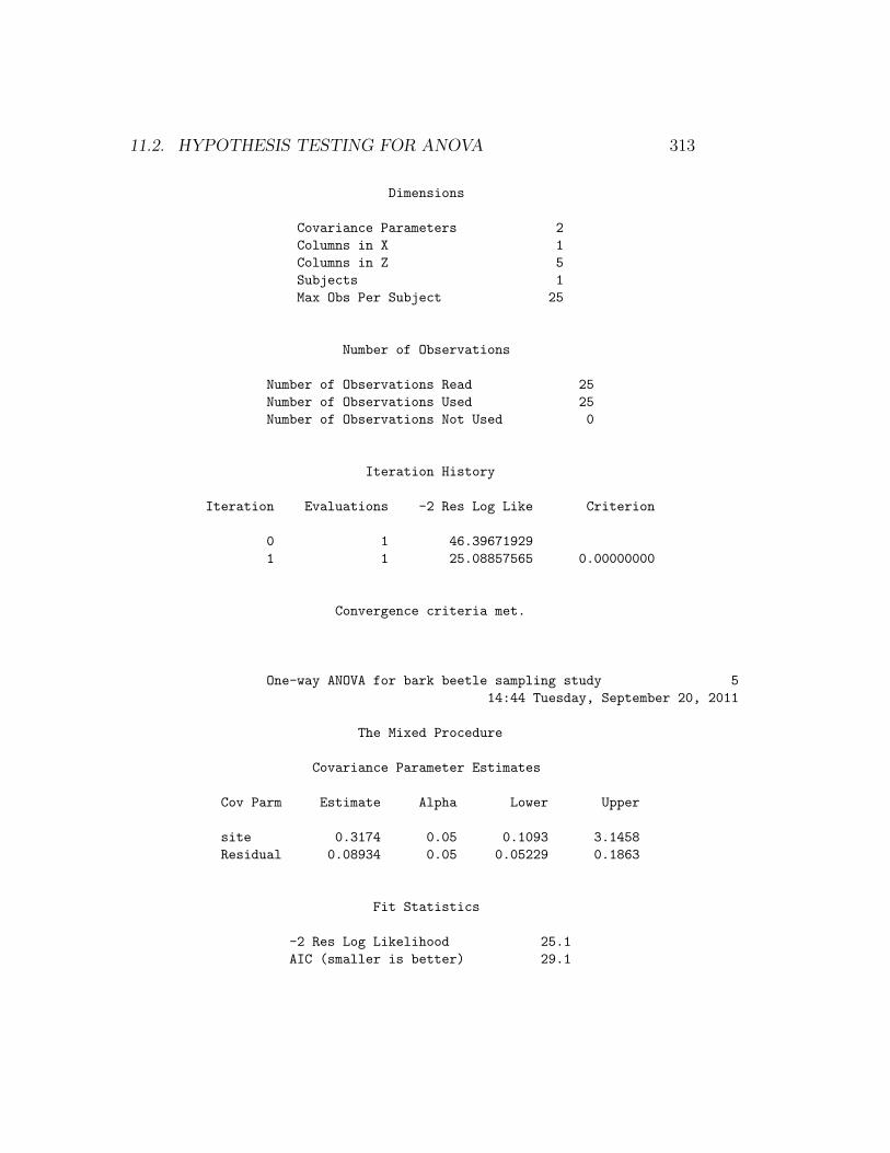
get only these estimates and no F test. Confidence intervals for the variancecomponents are requested using the cl option. The variance componentsestimated in the second proc mixed using a version of maximum likelihood,the preferred method of estimating these quantities.

The complete SAS program and output are listed below. The varianceamong sites is highly significant (F4,12 = 18.77, P < 0.0001. The second callto proc mixed provide estimates and confidence intervals for the two variancecomponents and confidence intervals. We have σ2

A = 0.3174 for which the95% confidence interval is (0.1093, 3.1458), and σ2 = 0.0893 with confidenceinterval (0.0523, 0.1863). From these results, we see that the variance amongsites is considerably greater than the variance within sites (0.3174 > 0.0893).

SAS Program

* bark_beetle_random.sas;


goptions reset=all;

title "One-way ANOVA for bark beetle sampling study";

data bark_beetle;

input site $ count;


y = log10(count);

datalines;

1 137

1 101

1 113

1 48

1 155

2 156

2 165

2 652

2 179

2 757

3 278

3 197

3 95

3 395

3 83

4 2540

4 613

4 200

4 251

4 390

5 18


5 16

5 11

5 21

5 14

;

run;

* Print data set;


run;



plot y*site=1 / vaxis=axis1 haxis=axis1;



run;

* One-way ANOVA with random effects - F test;

proc mixed method=type3 data=bark_beetle;

class site;

model y = / ddfm=kr;

random site;

run;

* One-way ANOVA with random effects - variance components;

proc mixed cl data=bark_beetle;

class site;

model y = / ddfm=kr outp=resids;

random site;

run;

goptions reset=all;

title "Diagnostic plots to check ANOVA assumptions";

* Plot residuals vs. predicted values;

proc gplot data=resids;

plot resid*pred=1 / vaxis=axis1 haxis=axis1;

symbol1 v=star height=2 width=3;


run;

* Normal quantile plot of residuals;

proc univariate noprint data=resids;

qqplot resid / normal waxis=3 height=4;

run;

quit;


SAS Output

One-way ANOVA for bark beetle sampling study 1

14:44 Tuesday, September 20, 2011

Obs site count y

1 1 137 2.13672

2 1 101 2.00432

3 1 113 2.05308

4 1 48 1.68124

5 1 155 2.19033

6 2 156 2.19312

7 2 165 2.21748

8 2 652 2.81425

9 2 179 2.25285

10 2 757 2.87910

11 3 278 2.44404

12 3 197 2.29447

13 3 95 1.97772

14 3 395 2.59660

15 3 83 1.91908

16 4 2540 3.40483

17 4 613 2.78746

18 4 200 2.30103

19 4 251 2.39967

20 4 390 2.59106

21 5 18 1.25527

22 5 16 1.20412

23 5 11 1.04139

24 5 21 1.32222

25 5 14 1.14613



The Mixed Procedure

Model Information

Data Set WORK.BARK_BEETLE

Dependent Variable y

Covariance Structure Variance Components

Estimation Method Type 3


Residual Variance Method Factor

Fixed Effects SE Method Kenward-Roger

Degrees of Freedom Method Kenward-Roger


Class Levels Values

site 5 1 2 3 4 5

Dimensions

Covariance Parameters 2

Columns in X 1

Columns in Z 5

Subjects 1

Max Obs Per Subject 25

Number of Observations



Number of Observations Not Used 0

Type 3 Analysis of Variance

Sum of

Source DF Squares Mean Square Expected Mean Square

site 4 6.706318 1.676580 Var(Residual) + 5 Var(site)

Residual 20 1.786777 0.089339 Var(Residual)

Type 3 Analysis of Variance

Error

Source Error Term DF F Value Pr > F

site MS(Residual) 20 18.77 <.0001

Residual . . . .




The Mixed Procedure

Covariance Parameter

Estimates

Cov Parm Estimate

site 0.3174

Residual 0.08934

Fit Statistics

-2 Res Log Likelihood 25.1

AIC (smaller is better) 29.1

AICC (smaller is better) 29.7

BIC (smaller is better) 28.3



The Mixed Procedure

Model Information

Data Set WORK.BARK_BEETLE

Dependent Variable y

Covariance Structure Variance Components

Estimation Method REML

Residual Variance Method Profile

Fixed Effects SE Method Kenward-Roger

Degrees of Freedom Method Kenward-Roger


Class Levels Values

site 5 1 2 3 4 5


Dimensions

Covariance Parameters 2

Columns in X 1

Columns in Z 5

Subjects 1

Max Obs Per Subject 25

Number of Observations



Number of Observations Not Used 0

Iteration History

Iteration Evaluations -2 Res Log Like Criterion

0 1 46.39671929

1 1 25.08857565 0.00000000

Convergence criteria met.



The Mixed Procedure

Covariance Parameter Estimates

Cov Parm Estimate Alpha Lower Upper

site 0.3174 0.05 0.1093 3.1458

Residual 0.08934 0.05 0.05229 0.1863

Fit Statistics

-2 Res Log Likelihood 25.1

AIC (smaller is better) 29.1


AICC (smaller is better) 29.7

BIC (smaller is better) 28.3

Figure 11.8: Means and standard errors for five study sites

11.3. MAXIMUM LIKELIHOOD ESTIMATES 315

11.3 Maximum likelihood estimates

This section sketches how the parameters in one-way ANOVA can be esti-mated using maximum likelihood. Recall that the likelihood for a randomsample of three observations (Y1 = 4.5, Y2 = 5.4, Y2 = 5.3) from a normaldistribution (see Chapter 8) was of the form

L(µ, σ2) =1√

2πσ2e−

12

(4.5−µ)2

σ2 × 1√2πσ2

e−12

(5.4−µ)2

σ2 × 1√2πσ2

e−12

(5.3−µ)2

σ2 .

(11.48)

We found maximum likelihood estimates of the normal distribution param-eters by maximizing this quantity with respect to µ and σ2.

Suppose now we have a data set that can be modeled using the fixedeffects one-way ANOVA model, in particular

Yij = µ+ αi + εij. (11.49)

This model has a number of parameters to estimate, such as µ, αi for i =1, 2, . . . , a, and σ2. What would the likelihood function look like for thesedata? Consider the first group for the bark beetle experiment (Example 1),for which we have Y11 = 2.576, Y12 = 2.10, Y13 = 2.41, Y14 = 2.14, andY15 = 2.58. For the first group the model assumes that Y1j ∼ N(µ+ α1, σ

2),and so the likelihood would be

L1 =1√

2πσ2e−

12

(2.57−(µ+α1))2

σ2 × 1√2πσ2

e−12

(2.10−(µ+α1))2

σ2 × 1√2πσ2

e−12

(2.41−(µ+α1))2

σ2

(11.50)

× 1√2πσ2

e−12

(2.14−(µ+α1))2

σ2 × 1√2πσ2

e−12

(2.58−(µ+α1))2

σ2 .

(11.51)

The likelihood L2 for the second group would be similar, except that Y2j ∼N(µ + α2, σ

2), and L3 similarly defined. The overall likelihood would thenbe defined as

L(µ, α1, α2, α3, σ2) = L1 × L2 × L3. (11.52)

Finding the maximum likelihood estimates involves maximizing this quan-tity with respect to the parameters µ, α1, α2, α3, and σ2. The likelihood for


designs with any number of treatment groups and replicates would be simi-lar. Using a bit of calculus to find the maximum, it can be shown that themaximum likelihood estimates of these parameters, in general, are

µ = ¯Y, (11.53)

αi = Yi· − ¯Y, (11.54)

and

σ2 =

∑ni=1


a(n− 1)= MSwithin. (11.55)

(McCulloch & Searle 2001). These estimators seem quite reasonable. Theyuse the grand mean of the data, ¯Y , to estimate the grand mean µ of themodel, and the difference between the ith group mean and the grand mean,Yi· − ¯Y , to estimate the deviation from the group mean αi. Note that σ2

is equal to MSwithin, which we have already encountered in our ANOVAcalculations.

Suppose now we have a data set suited to the random effects model, inparticular

Yij = µ+ Ai + εij. (11.56)

This model has three parameters to be estimated: µ, σ2A, and σ2. The

likelihood for this model is more complex because of the random effect Ai, butone can show that the maximum likelihood estimators of these parametersare

µ = ¯Y, (11.57)

σ2A =

MSamong −MSwithinn

, (11.58)

andσ2 = MSwithin. (11.59)

An intuitive explanation of the formula for σ2A is that MSamong incorporates

variance from both Ai and εij, while MSwithin only has εij. SubtractingMSwithin from MSamong leaves only the variance due to Ai, so that the nu-merator of this expression estimates nσ2

A. We then divide by n to obtain anestimate of σ2

A.Suppose that for an unusual data set we obtain MSamong < MSwithin,

implying a negative estimate of σ2A = 0 according to the above equation. An

inherent feature of maximum likelihood is that is restricts variance compo-nents to plausible values (McCulloch & Searle 2001), so in this case it would

11.4. F TEST AS A LIKELIHOOD RATIO TEST 317

simply say that σ2A = 0, the smallest possible nonnegative value. This would

be reflected in the SAS output for proc mixed, which would report that thevariance component in question was zero. The estimates presented here areactually obtained using a variant of maximum likelihood called restrictedmaximum likelihood or REML. This method is the default in SAS, and hassome theoretical advantages over straight maximum likelihood (McCullochand Searle 2001).

11.4 F test as a likelihood ratio test

The F test in one-way ANOVA can be derived as a likelihood ratio test, simi-lar to the development of the t test in Chapter 10. We first find the maximumlikelihood estimates of various parameters under H1 vs. H0, where the pa-rameters under consideration are the ANOVA model parameters. Recall thatthe observations in the fixed effects model are described as

Yij = µ+ αi + εij (11.60)

where µ is the grand mean, αi is the effect of the ith treatment, and εij ∼N(0, σ2). This is the statistical model under the alternative hypothesis,where αi 6= 0 for some i. Under H0 : all αi = 0, the model reduces tojust

Yij = µ+ εij. (11.61)

We would need to find the maximum likelihood estimates under both H1 (seeprevious section) and H0, as well as LH0 and LH1 , the maximum height ofthe likelihood function under H0 and H1. We would then use the likelihoodratio test statistic

λ =LH0

LH1

. (11.62)

It can be shown that there is a one-to-one correspondence between −2 ln(λ)and Fs in one-way ANOVA, and so the F test is actually a likelihood ratio test(McCulloch & Searle 2001). A similar argument can be made to justify the Ftest for the random effects model. Like all likelihood ratio tests, large valuesof the test statistic −2 ln(λ) or Fs indicate a lower value of the likelihoodunder H0 relative to H1, and thus a poorer fit of the H0 model.


11.5 One-way ANOVA and two-sample t tests

There is an alternative to one-way ANOVA when there are only two groupsto be compared, the two-sample t test. Let µ1 be the mean of the first groupand µ2 the second one, and suppose that the two groups have the samevariance σ2 and sample size n. We are interested in testing H0 : µ1 = µ2 vs.H1 : µ1 6= µ2, to determine if there are differences in the means of the twogroups. Under H0, the test statistic

Ts =(Y1· − Y2·)√

s21+s222

∼ t2(n−1). (11.63)

Here Y1· and Y2 are the sample means for each group, and s21 and s2

2 thesample variances. For a Type I error rate of α, the acceptance region of thetest would be the interval (−cα,2(n−1), cα,2(n−1)), where cα,2(n−1) is determinedusing Table T (see Chapter 10). We would reject H0 if it falls on the edge oroutside this interval. There are also versions of this test statistic for unequalsample sizes.

Although a two-sample t test is often used for comparing two groups, inthe form above it is equivalent to the F test in one-way ANOVA. To seethis, note that T 2

s = Fs for one-way ANOVA with two groups. It can alsobe shown that the acceptance and rejection regions are the same for thetwo tests. Unlike ANOVA, though, a two-sample t test can also be used forone-tailed alternative hypotheses, such as H1 : µ1 > µ2 or H1 : µ1 < µ2.The procedure is similar to one-sample t tests for one-tailed alternatives (seeChapter 10).

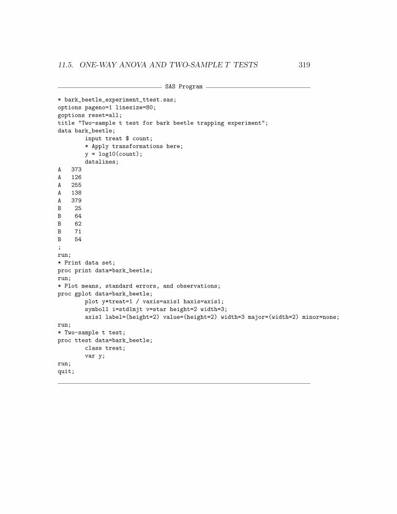
11.5.1 Two-sample t test for Example 1 - SAS demo

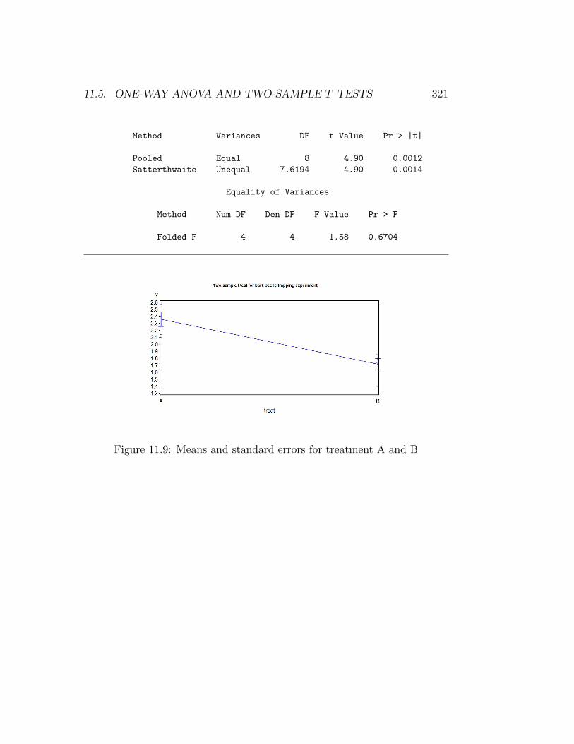
We can illustrate this test by comparing treatment A and B in the Example1 study, deleting the data for the third treatment. See SAS program andoutput below. The data and proc gplot portions of the program are similarto our previous one-way ANOVA code. The two-sample t test is carried usingproc ttest (SAS Institute Inc. 2014a), with the class statement indicatingthe variable that codes for different groups (treat), while the var statementdesignates the dependent variable (y). We see there is a highly significant dif-ference between treatment A and B (t8 = 4.90, P = 0.0012), with treatmentA catching more beetles than B (Fig. 11.9).

11.5. ONE-WAY ANOVA AND TWO-SAMPLE T TESTS 319

SAS Program

* bark_beetle_experiment_ttest.sas;


goptions reset=all;

title "Two-sample t test for bark beetle trapping experiment";

data bark_beetle;



y = log10(count);

datalines;

A 373

A 126

A 255

A 138

A 379

B 25

B 64

B 62

B 71

B 54

;

run;

* Print data set;


run;






run;

* Two-sample t test;

proc ttest data=bark_beetle;

class treat;

var y;

run;

quit;


SAS Output

Two-sample t test for bark beetle trapping experiment 1

16:16 Thursday, May 22, 2014

Obs treat count y

1 A 373 2.57171

2 A 126 2.10037

3 A 255 2.40654

4 A 138 2.13988

5 A 379 2.57864

6 B 25 1.39794

7 B 64 1.80618

8 B 62 1.79239

9 B 71 1.85126

10 B 54 1.73239

s

Two-sample t test for bark beetle trapping experiment 2

16:16 Thursday, May 22, 2014

The TTEST Procedure

Variable: y

treat N Mean Std Dev Std Err Minimum Maximum

A 5 2.3594 0.2295 0.1026 2.1004 2.5786

B 5 1.7160 0.1828 0.0818 1.3979 1.8513

Diff (1-2) 0.6434 0.2075 0.1312

treat Method Mean 95% CL Mean Std Dev

A 2.3594 2.0745 2.6444 0.2295

B 1.7160 1.4890 1.9430 0.1828

Diff (1-2) Pooled 0.6434 0.3408 0.9460 0.2075

Diff (1-2) Satterthwaite 0.6434 0.3382 0.9486

treat Method 95% CL Std Dev

A 0.1375 0.6594

B 0.1095 0.5253

Diff (1-2) Pooled 0.1401 0.3975

Diff (1-2) Satterthwaite

11.5. ONE-WAY ANOVA AND TWO-SAMPLE T TESTS 321

Method Variances DF t Value Pr > |t|

Pooled Equal 8 4.90 0.0012

Satterthwaite Unequal 7.6194 4.90 0.0014

Equality of Variances

Method Num DF Den DF F Value Pr > F

Folded F 4 4 1.58 0.6704

Figure 11.9: Means and standard errors for treatment A and B


11.6 References

McCulloch, C. E. & Searle, S. R. (2001) Generalized, Linear, and MixedModels. John Wiley & Sons, Inc., New York, NY.

Littell, R. C., Milliken, G. A., Stroup, W. W. & Wolfinger, R. D. (1996) TheSAS System for Mixed Models. SAS Institute Inc., Cary, NC.

SAS Institute Inc. (2014a) SAS/STAT 13.2 Users Guide. SAS Institute Inc.,Cary, NC.

SAS Institute Inc. (2014b) SAS/GRAPH 9.4: Reference, Third Edition.SAS Institute Inc., Cary, NC.

Winer, B. J., Brown, D. R. & Michels, K. M. (1991) Statistical Principles inExperimental Design, 3rd edition. McGraw-Hill, Inc., Boston, MA.

11.7. PROBLEMS 323

11.7 Problems

1. A doctor conducts an experiment in which men are placed on fourdifferent diets, consisting of a standard weight loss regimen (a controltreatment) and three new diets (Diets 1, 2, 3). The weight losses (lbs)after six months are given in the following table.

Control Diet 1 Diet 2 Diet 319.5 20.0 20.8 25.920.5 16.4 17.4 25.916.6 11.9 16.7 25.819.3 22.1 16.8 22.5

(a) Test whether there is a significant difference among the four treat-ments using one-way ANOVA, using manual calculations. Reportthe P value and discuss the significance of the test, and then in-terpret the results of the experiment. Show all your calculations.

(b) Repeat the analysis using SAS and proc glm. Attach your programand output.

2. An experiment was conducted on the fecundity of a predatory insectreared on an artificial diet using four different concentrations of thepreservative sorbic acid: (1) no sorbic acid, (2) 0.1% sorbic acid, (3)0.2% sorbic acid, and (4) 0.5% sorbic acid. Twenty insects were rearedat each concentration and the fecundity of the resulting adults mea-sured. See table below.

Treatment ObservationsNo sorbic acid 87, 124, 105, 87, 100, 89, 95, 79, 102, 112

92, 87, 115, 96, 111, 90, 86, 92, 109, 760.1% sorbic acid 105, 94, 97, 94, 83, 97, 107, 99, 104, 83

101, 71, 100, 75, 87, 106, 88, 99, 90, 740.2% sorbic acid 73, 94, 81, 83, 100, 98, 76, 91, 68, 82

92, 105, 76, 82, 95, 96, 101, 89, 92, 670.5% sorbic acide 83, 54, 86, 76, 74, 81, 79, 72, 80, 78

70, 83, 83, 85, 90, 70, 85, 94, 82, 75

Test whether there is a difference among the four treatments using one-way ANOVA and SAS. Interpret the results of this analysis, providinga P value and discussing the significance of the test. Using a graph,


explain what happens to fecundity as the concentration of sorbic acidchanges.

Chapter 11 Analysis of Variance (One-Way) - · PDF fileChapter 11 Analysis of Variance...

Documents

Transcript of Chapter 11 Analysis of Variance (One-Way) - · PDF fileChapter 11 Analysis of Variance...