Chapter 10 Hypothesis Testing - · PDF filethis chapter, we examine the ... 250 CHAPTER 10....

Chapter 10

Hypothesis Testing

We previously examined how the parameters for a probability distributioncan be estimated using a random sample and maximum likelihood (Chapter8), as then showed how confidence intervals provide a measure of the relia-bility of these estimates (Chapter 9). In hypothesis testing, the subject ofthis chapter, we examine the consistency of observed data sets with a nullhypothesis, commonly a statement about the parameter values within a sta-tistical model. We conduct a statistical test of this null hypothesis, withthe result being a decision to accept or reject the null hypothesis based onthe magnitude of a quantity called a P value. Small values of P indicate atest result inconsistent with the null hypothesis, suggesting it might be falseand some alternative hypothesis more valid. In the following, we discuss thedifferent components and steps of hypothesis testing.

10.1 The null and alternative hypotheses

As an example of hypothesis testing, suppose that we rear n tilapia on acommercial diet, and want to compare their body size with ones reared usinga natural diet. Fish reared on natural food are already known to have aweight of 500 g at a certain age, and weight is normally distributed. Wecould test whether the fish reared on the commercial diet have the same meanweight as ones reared on natural food (500 g) using the null hypothesis thatµ = 500 g, where µ is the mean parameter for the normal distribution. Thiscan be written as H0 : µ = 500 g, where H0 stands for null hypothesis. Nullhypotheses of this type can be written more generally as H0 : µ = µ0, where

245

246 CHAPTER 10. HYPOTHESIS TESTING

µ0 is the hypothesized mean of the distribution. For the tilapia problem, wewould have µ0 = 500 g.

An alternative hypothesis for this example is that the mean weight oftilapia on commercial diet is different from 500 g. This can be written asH1 : µ 6= 500 g, where H1 stands for the alternative hypothesis. Alternativehypotheses of this type are written generally as H1 : µ 6= µ0. We may also beinterested in particular values of the alternative mean, such as H1 : µ = 490g or H1 : µ = 530 g, or more generally H1 : µ = µ1.

10.2 Test statistics

A test statistic is a quantity that measures the consistency of theobserved data with the null hypothesis. Test statistics are usuallychosen so that large values occur when the data are inconsistent with H0.What would be a suitable test statistic for the tilapia problem, using H0 :µ = µ0 as the null hypothesis? Suppose we rear n fish on the commercialdiet, and then calculate the sample mean Y of their weights. The statisticY is an estimator of the true mean µ for this statistical population, whichmay or may not be equal to the µ0 under the null hypothesis. A value ofY substantially greater than µ0, or smaller than µ0, would be inconsistentwith H0. This suggests using the quantity Y −µ0 as the test statistic for theproblem. What about the other parameter for the normal distribution, σ2 orσ? For simplicity, we will assume that it is a known quantity, although thisis rare in practice. We will then employ the test statistic

Zs =Y − µ0

σ/√n

(10.1)

to test H0 : µ = µ0 (Bickel & Doksum 1977). We use this statistic becauseit has a standard normal distribution under H0 (Zs ∼ N(0, 1), see Chapter9) which makes it straightforward to employ the test. Note that Zs becomeslarge (positive or negative) if the sample mean Y differs greatly from µ0.Tests based on the standard normal distribution are called Z tests.

10.3. ACCEPTANCE AND REJECTION REGIONS – TYPE I ERROR247

10.3 Acceptance and rejection regions – Type

I error

Given a suitable test statistic, how large must it be before we decide thedata are inconsistent with H0? This is determined by finding an intervalthat defines an acceptance region for the test, and its complement, calledthe rejection or critical region (Bickel & Doksum 1977). We then acceptH0 if the test statistic falls within the acceptance region, and reject H0 if itfalls outside or lies on its boundary. The boundaries of the acceptance andrejection regions are determined by setting the probability of a Type I error.A Type I error is defined as the test rejecting H0 when H0 is true.The probability of committing a Type I error is called the Type Ierror rate, usually denoted with the symbol α. It is common practiceto set α = 0.05, meaning there is a 1 in 20 chance that the test will rejectH0 even when it is true. It follows that the probability of the test acceptingH0 if it is true is 1− α. For α = 0.05, we have 1− α = 1− 0.05 = 0.95.

The acceptance region is determined as follows. Suppose that H0 : µ = µ0

is true. Because the test statistic Zs ∼ N(0, 1) under H0, the following is atrue statement:

P [−cα < Zs < cα] = P [−cα <Y − µ0

σ/√n< cα] = 1− α. (10.2)

The quantity cα would be chosen using Table Z to satisfy this equation (fordetails see Chapter 9). The interval (−cα, cα) is the acceptance region of atest with a Type I error rate of α. Under H0, the test statistic Zs wouldlie within this interval with probability 1 − α and outside this region withprobability α, which is the required Type I error rate. The rejection regionwould be the complement of the acceptance region, i.e., all values on theboundary or outside of (−cα, cα).

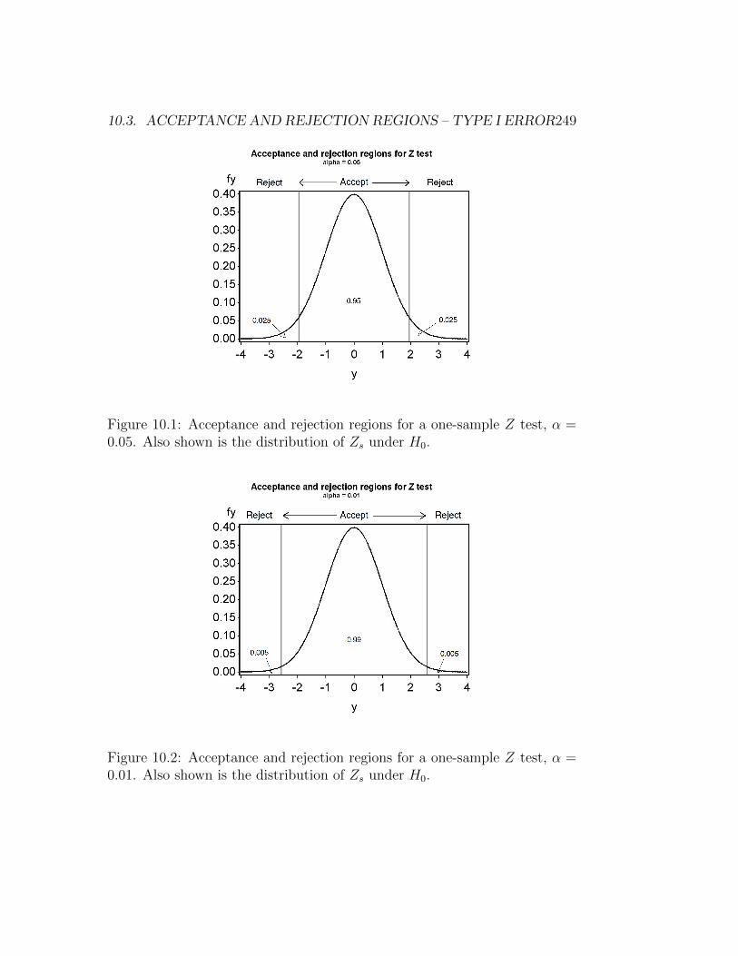
For example, with α = 0.05 we find that c0.05 = 1.96, and so we wouldaccept H0 if Zs lies within (−1.96, 1.96) and reject H0 if it lies outside thisinterval or exactly on the boundary (see Fig. 10.1). The acceptance regionfor this test can also be expressed using absolute values - we would acceptH0 if |Zs| < 1.96 and reject it if |Zs| ≥ 1.96.

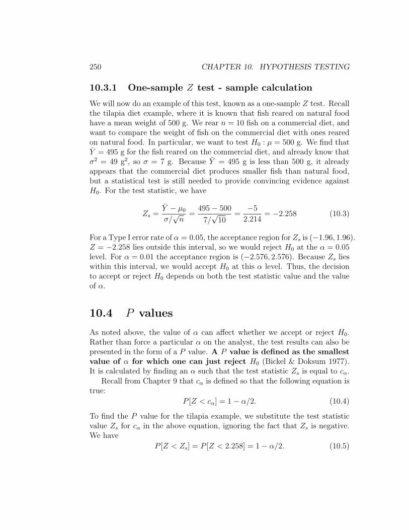
The acceptance region becomes larger (and the rejection region smaller)for smaller α values. For α = 0.01, we find that c0.01 = 2.576 and so theacceptance region is (−2.576, 2.576) (Fig. 10.2). Using absolute values, we


would accept H0 if |Zs| < 2.576 and reject it otherwise. Using a smallervalue of α indicates we are more concerned about making a Type I error.For α = 0.01 there is only a 1 in 100 chance we would reject H0 if H0 weretrue, but this also reduces the power of the test (see below) to detect whetherH0 is false.

The acceptance and rejection regions we just developed are for a two-tailed test, which tests the null hypothesis H0 : µ = µ0 with H1 : µ 6= µ0

the alternative hypothesis. This test statistic will reject H0 for either largeand small values of the test statistic Zs, which occurs when Y is greater thanµ0 or less than µ0. We will later examine the behavior of one-tailed tests,where the null is H0 : µ = µ0 while the alternative is of the form H1 : µ > µ0,or H1 : µ < µ0. Note that the two alternative hypotheses here specify thatµ is either greater or less than µ0.

10.3. ACCEPTANCE AND REJECTION REGIONS – TYPE I ERROR249

Figure 10.1: Acceptance and rejection regions for a one-sample Z test, α =0.05. Also shown is the distribution of Zs under H0.

Figure 10.2: Acceptance and rejection regions for a one-sample Z test, α =0.01. Also shown is the distribution of Zs under H0.


10.3.1 One-sample Z test - sample calculation

We will now do an example of this test, known as a one-sample Z test. Recallthe tilapia diet example, where it is known that fish reared on natural foodhave a mean weight of 500 g. We rear n = 10 fish on a commercial diet, andwant to compare the weight of fish on the commercial diet with ones rearedon natural food. In particular, we want to test H0 : µ = 500 g. We find thatY = 495 g for the fish reared on the commercial diet, and already know thatσ2 = 49 g2, so σ = 7 g. Because Y = 495 g is less than 500 g, it alreadyappears that the commercial diet produces smaller fish than natural food,but a statistical test is still needed to provide convincing evidence againstH0. For the test statistic, we have

Zs =Y − µ0

σ/√n

=495− 500

7/√

10=−5

2.214= −2.258 (10.3)

For a Type I error rate of α = 0.05, the acceptance region for Zs is (−1.96, 1.96).Z = −2.258 lies outside this interval, so we would reject H0 at the α = 0.05level. For α = 0.01 the acceptance region is (−2.576, 2.576). Because Zs lieswithin this interval, we would accept H0 at this α level. Thus, the decisionto accept or reject H0 depends on both the test statistic value and the valueof α.

10.4 P values

As noted above, the value of α can affect whether we accept or reject H0.Rather than force a particular α on the analyst, the test results can also bepresented in the form of a P value. A P value is defined as the smallestvalue of α for which one can just reject H0 (Bickel & Doksum 1977).It is calculated by finding an α such that the test statistic Zs is equal to cα.

Recall from Chapter 9 that cα is defined so that the following equation istrue:

P [Z < cα] = 1− α/2. (10.4)

To find the P value for the tilapia example, we substitute the test statisticvalue Zs for cα in the above equation, ignoring the fact that Zs is negative.We have

P [Z < Zs] = P [Z < 2.258] = 1− α/2. (10.5)

10.4. P VALUES 251

From Table Z, we see that P [Z < 2.258] ≈ 0.9881. We then solve theequation

0.9881 = 1− α/2 (10.6)

for α to obtain the P value. We have α = 2(1 − 0.9881) = 0.0238. Thisis the P value for the test, reported as P = 0.0238. Given the P value,the analyst or other interested parties can decide for themselves whether toreject or accept H0.

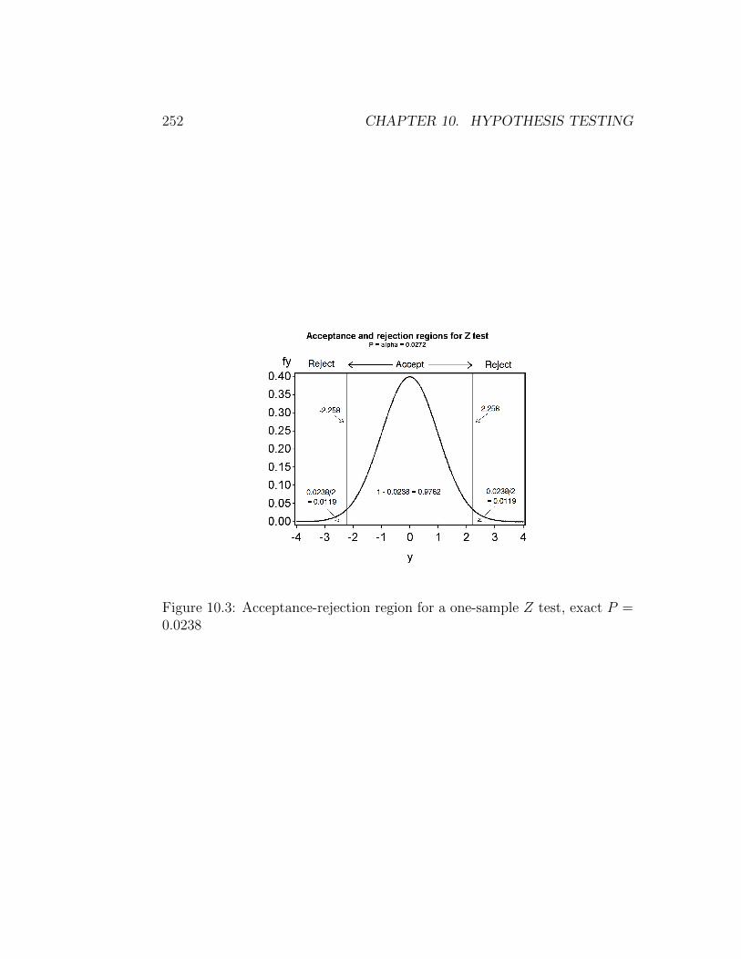
A P value can also be thought of as the probability of obtaininga test statistic equal to or more extreme than the observed one,under the null hypothesis. We can see this from a graph of the accep-tance and rejection regions for the tilapia example, where Zs = −2.258 andP = 0.0238 (Fig. 10.3). The probabilities outside the acceptance region cor-respond to P [Zs ≤ −2.258] and P [Zs ≥ 2.258], which are the probabilitiesof observing values of Zs equal to or more extreme than the observed valueof Zs = −2.258. The two definitions of a P value are equivalent.

A P value is also a measure of the consistency of the observeddata with the null hypothesis. If the P value is large, say P > 0.05, thenthe observed data generated a test statistic value that is fairly likely underthe null hypothesis. On the other hand, if P is small then the observed datahas generated a test statistic that is unlikely under the null hypothesis. Thissuggests the observed data are inconsistent with the null hypothesis, and thenull may be false.

There are specific phrases generally used to describe the significance ofa statistical test result. If a test yields P ≤ 0.05, it is described as beingsignificant, while if P ≤ 0.01 it is highly significantly. If P > 0.05 the testis described as nonsignificant. The tilapia example with P = 0.0272 wouldbe described as significant because 0.0272 < 0.05, but not highly significant.


Figure 10.3: Acceptance-rejection region for a one-sample Z test, exact P =0.0238

10.5. TYPE II ERROR AND POWER 253

10.5 Type II error and power

Suppose now that H0 is actually false and some alternative hypothesis H1 istrue. A Type II error is defined as failing to reject H0 when H0 isfalse. The probability of committing a Type II error is called the Type IIerror rate, usually denoted by the symbol β. It follows that the probabilityof the test rejecting H0 if it is false is 1 − β, and this quantity is called thepower of the test (Bickel & Doksum 1977). High power values indicate thetest is capable of detecting departures from the null hypothesis.

The power and Type II error rate of a statistical test depends on thesample size n of the test, the standard deviation of the observations σ, theType I error rate α, and the particular alternative hypothesis chosen. Ananalyst interested in determining the power of a test will fix some of thesevalues, often α and σ, and then examine how changes in n and the alternativehypothesis affect power. This procedure is called a power analysis. A powervalue of 0.8 is believed to be adequate in most situations (Cohen 1988). Thisimplies that a statistical test will reject H0 when it is false 80% of the time.

It is relatively easy to calculate the power for a one-sample Z test, usingthe distribution of Zs under H1. Suppose that we choose α = 0.05, so thatthe acceptance region is the interval (−1.96, 1.96), and that the alternativehypothesis is H1 : µ = µ1 for some µ1. Under H0 : µ = µ0 the test statistichas a standard normal distribution, implying Zs ∼ N(0, 1), but what isits distribution under H1? Using the expected value and variance rules inChapter 7, one can show that

E[Zs] =µ1 − µ0

σ/√n

= φ (10.7)

and also that V ar[Zs] = 1. So, Zs has the same variance under both H1 andH0, but the mean under H1 is equal to φ, not zero as under H0. It followsthat under H1 the test statistic Zs ∼ N(φ, 1). The probability of rejectingH0 when H1 is true, the power of the test, is the probability that Zs liesoutside the interval (−1.96, 1.96), or

power = P [Zs ≤ −1.96] + P [Zs ≥ 1.96]. (10.8)

The Type II error rate β can be calculated as 1−power, or directly by finding

β = P [−1.96 < Zs < 1.96] (10.9)


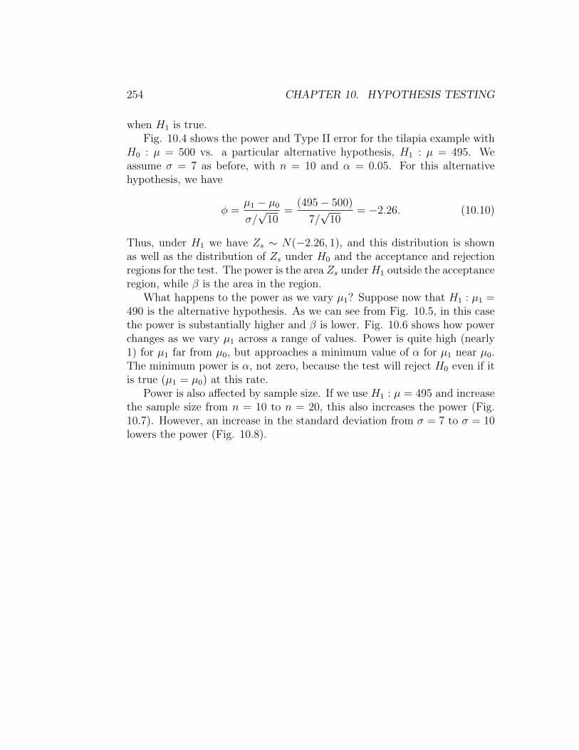
when H1 is true.Fig. 10.4 shows the power and Type II error for the tilapia example with

H0 : µ = 500 vs. a particular alternative hypothesis, H1 : µ = 495. Weassume σ = 7 as before, with n = 10 and α = 0.05. For this alternativehypothesis, we have

φ =µ1 − µ0

σ/√

10=

(495− 500)

7/√

10= −2.26. (10.10)

Thus, under H1 we have Zs ∼ N(−2.26, 1), and this distribution is shownas well as the distribution of Zs under H0 and the acceptance and rejectionregions for the test. The power is the area Zs under H1 outside the acceptanceregion, while β is the area in the region.

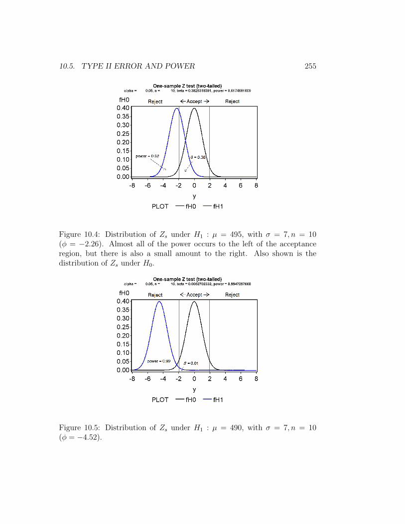
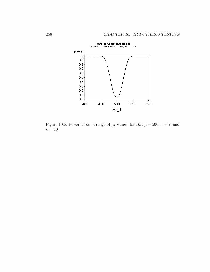
What happens to the power as we vary µ1? Suppose now that H1 : µ1 =490 is the alternative hypothesis. As we can see from Fig. 10.5, in this casethe power is substantially higher and β is lower. Fig. 10.6 shows how powerchanges as we vary µ1 across a range of values. Power is quite high (nearly1) for µ1 far from µ0, but approaches a minimum value of α for µ1 near µ0.The minimum power is α, not zero, because the test will reject H0 even if itis true (µ1 = µ0) at this rate.

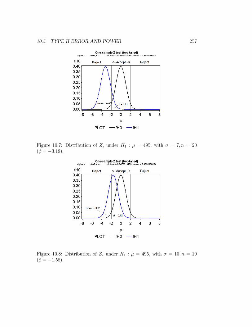
Power is also affected by sample size. If we use H1 : µ = 495 and increasethe sample size from n = 10 to n = 20, this also increases the power (Fig.10.7). However, an increase in the standard deviation from σ = 7 to σ = 10lowers the power (Fig. 10.8).


Figure 10.4: Distribution of Zs under H1 : µ = 495, with σ = 7, n = 10(φ = −2.26). Almost all of the power occurs to the left of the acceptanceregion, but there is also a small amount to the right. Also shown is thedistribution of Zs under H0.

Figure 10.5: Distribution of Zs under H1 : µ = 490, with σ = 7, n = 10(φ = −4.52).


Figure 10.6: Power across a range of µ1 values, for H0 : µ = 500, σ = 7, andn = 10


Table 10.1: Effects on power and the Type II error rate β of changes invarious parameters. The arrows indicate if a particular quantity increases ordecreases.

Parameter Direction φ power β|µ1 − µ0| ↑ ↑ ↑ ↓

n ↑ ↑ ↑ ↓σ ↑ ↓ ↓ ↑α ↑ no change ↑ ↓

All of these effects on power can be understood through their influenceon φ. Any change in a parameter value that makes φ larger increases powerand reduces β, because it shifts the distribution of Zs under H1 away fromthe acceptance and into the rejection region. Thus, large differences betweenµ1 and µ0, large n, and small σ will all increase power because they increaseφ. Conversely, similar values of µ1 and µ0, small n, and large σ would allreduce power. Table 10.1 summarizes how the different parameter valuesinfluence φ, power, and the Type II error rate β. Also shown is the effect ofthe Type I error rate α on power. If an investigator can accept a larger valueof α, so that Type I errors are more common, this reduces the acceptanceand increases the rejection region size, and thus increases power.

Note that a sufficiently large value of n can generate a large value of φ,even when µ1 and µ0 are close or σ is large. Thus, large sample sizes canyield adequate power even when the data are noisy, or the two means aresimilar in value. This basically arises from the inverse relationship betweenthe variance of Y and n, i.e., V ar[Y ] = σ2/n, which is incorporated in thetest statistic Zs (see Eqn. 10.1).

10.6 Summary table

A common way of summarizing the different outcomes in hypothesis testingis the table below. The null hypothesis H0 can be either true or false. If H0

is true, then the test may accept H0 and make a correct decision, or reject itand make a Type I error, with a Type I error rate of α. If H0 is false, thenthe test may accept H0 and make a Type II error with an error rate of β, orreject it and make a correct decision.

10.7. ONE-SAMPLE T TEST 259

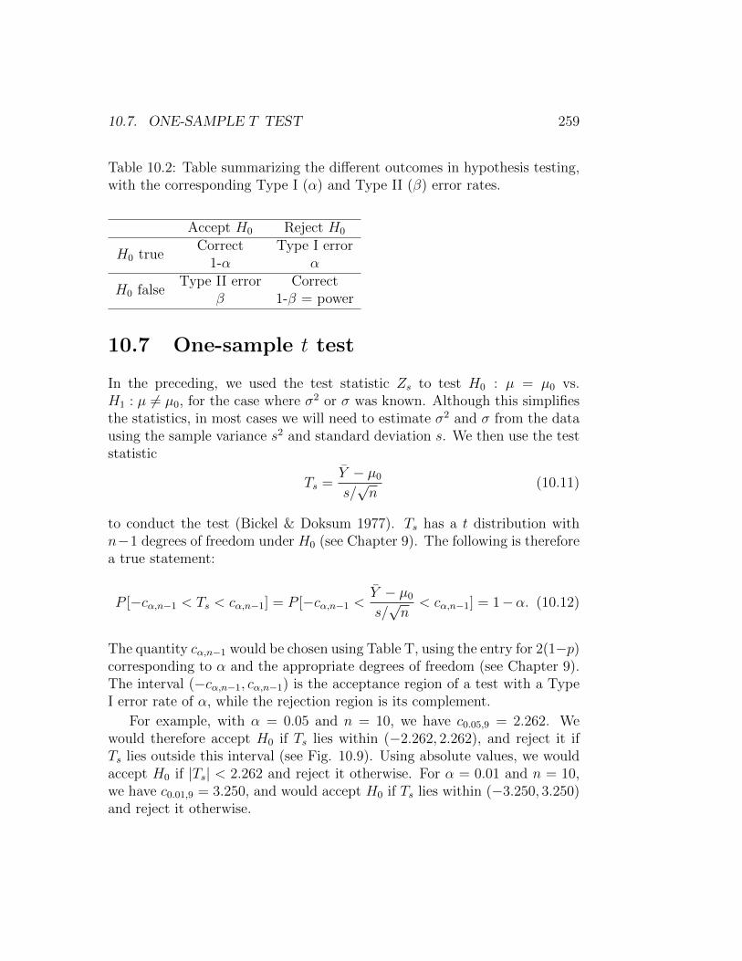
Table 10.2: Table summarizing the different outcomes in hypothesis testing,with the corresponding Type I (α) and Type II (β) error rates.

Accept H0 Reject H0

H0 trueCorrect Type I error

1-α α

H0 falseType II error Correct

β 1-β = power

10.7 One-sample t test

In the preceding, we used the test statistic Zs to test H0 : µ = µ0 vs.H1 : µ 6= µ0, for the case where σ2 or σ was known. Although this simplifiesthe statistics, in most cases we will need to estimate σ2 and σ from the datausing the sample variance s2 and standard deviation s. We then use the teststatistic

Ts =Y − µ0

s/√n

(10.11)

to conduct the test (Bickel & Doksum 1977). Ts has a t distribution withn−1 degrees of freedom under H0 (see Chapter 9). The following is thereforea true statement:

P [−cα,n−1 < Ts < cα,n−1] = P [−cα,n−1 <Y − µ0

s/√n

< cα,n−1] = 1−α. (10.12)

The quantity cα,n−1 would be chosen using Table T, using the entry for 2(1−p)corresponding to α and the appropriate degrees of freedom (see Chapter 9).The interval (−cα,n−1, cα,n−1) is the acceptance region of a test with a TypeI error rate of α, while the rejection region is its complement.

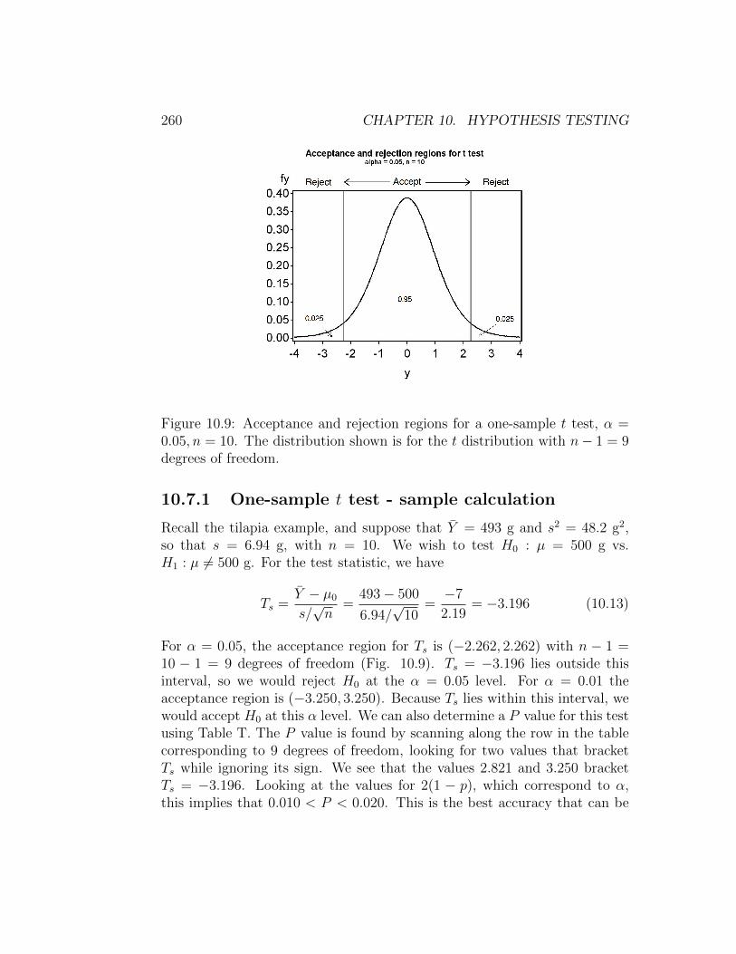
For example, with α = 0.05 and n = 10, we have c0.05,9 = 2.262. Wewould therefore accept H0 if Ts lies within (−2.262, 2.262), and reject it ifTs lies outside this interval (see Fig. 10.9). Using absolute values, we wouldaccept H0 if |Ts| < 2.262 and reject it otherwise. For α = 0.01 and n = 10,we have c0.01,9 = 3.250, and would accept H0 if Ts lies within (−3.250, 3.250)and reject it otherwise.


Figure 10.9: Acceptance and rejection regions for a one-sample t test, α =0.05, n = 10. The distribution shown is for the t distribution with n− 1 = 9degrees of freedom.

10.7.1 One-sample t test - sample calculation

Recall the tilapia example, and suppose that Y = 493 g and s2 = 48.2 g2,so that s = 6.94 g, with n = 10. We wish to test H0 : µ = 500 g vs.H1 : µ 6= 500 g. For the test statistic, we have

Ts =Y − µ0

s/√n

=493− 500

6.94/√

10=−7

2.19= −3.196 (10.13)

For α = 0.05, the acceptance region for Ts is (−2.262, 2.262) with n − 1 =10 − 1 = 9 degrees of freedom (Fig. 10.9). Ts = −3.196 lies outside thisinterval, so we would reject H0 at the α = 0.05 level. For α = 0.01 theacceptance region is (−3.250, 3.250). Because Ts lies within this interval, wewould accept H0 at this α level. We can also determine a P value for this testusing Table T. The P value is found by scanning along the row in the tablecorresponding to 9 degrees of freedom, looking for two values that bracketTs while ignoring its sign. We see that the values 2.821 and 3.250 bracketTs = −3.196. Looking at the values for 2(1 − p), which correspond to α,this implies that 0.010 < P < 0.020. This is the best accuracy that can be


accomplished using Table T, and to obtain an exact P value would requirethe use of SAS.

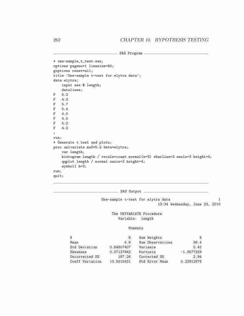
10.7.2 Hypothesis testing - SAS demo

We will use a small subset of our larger data set on elytra length (of thepredatory beetle Thanasimus dubius) to illustrate hypothesis testing usingSAS. The data are from a rearing study of insects reared on an artificial diet,and we want to compare their size to wild individuals. The subset data arefor eight female T. dubius and are listed below:

5.2 4.2 5.7 5.4 4.0 4.5 5.2 4.2

Suppose that wild predators have an elytral length of 5.2 mm. This suggeststesting H0 : µ = 5.2 mm vs. H1 : µ 6= 5.2 mm. We can conduct a one-samplet test for this null hypothesis using proc univariate, by adding the optionmu0=5.2 as an option. See SAS program and output listed below. The teststatistic Ts and its P value are listed on one line in SAS output:

Student’s t t -1.74574 Pr > |t| 0.1244

We see that Ts = −1.75 for this test. What is its P value? The notationPr > |t| in the printout is shorthand for the P [Ts < −1.75]+P [Ts > 1.75], theP value for this two-tailed test. We thus have P = 0.1244, a non-significanttest result because P > 0.05. The degrees of freedom for the test are notreported by SAS, but are equal to n− 1 = 8− 1 = 7. A sentence reportingthis test result in a scientific journal would be something like ‘A one-samplet test comparing the elytra length of individuals reared on artificial diet vs.wild individuals was non-significant (t7 = −1.75, P = 0.1244).’ Note thatthe degrees of freedom are reported as a subscript on the test statistic.


SAS Program

* one-sample_t_test.sas;

options pageno=1 linesize=80;

goptions reset=all;

title ’One-sample t-test for elytra data’;

data elytra;

input sex $ length;

datalines;

F 5.2

F 4.2

F 5.7

F 5.4

F 4.0

F 4.5

F 5.2

F 4.2

;

run;

* Generate t test and plots;

proc univariate mu0=5.2 data=elytra;

var length;

histogram length / vscale=count normal(w=3) wbarline=3 waxis=3 height=4;

qqplot length / normal waxis=3 height=4;

symbol1 h=3;

run;

quit;

SAS Output

One-sample t-test for elytra data 1

13:34 Wednesday, June 23, 2010

The UNIVARIATE Procedure

Variable: length

Moments

N 8 Sum Weights 8

Mean 4.8 Sum Observations 38.4

Std Deviation 0.64807407 Variance 0.42

Skewness 0.07137842 Kurtosis -1.9577259

Uncorrected SS 187.26 Corrected SS 2.94

Coeff Variation 13.5015431 Std Error Mean 0.22912878


Basic Statistical Measures

Location Variability

Mean 4.800000 Std Deviation 0.64807

Median 4.850000 Variance 0.42000

Mode 4.200000 Range 1.70000

Interquartile Range 1.10000

Note: The mode displayed is the smallest of 2 modes with a count of 2.

Tests for Location: Mu0=5.2

Test -Statistic- -----p Value------

Student’s t t -1.74574 Pr > |t| 0.1244

Sign M -1 Pr >= |M| 0.6875

Signed Rank S -7.5 Pr >= |S| 0.1563

Quantiles (Definition 5)

Quantile Estimate

100% Max 5.70

99% 5.70

95% 5.70

90% 5.70

75% Q3 5.30

50% Median 4.85

25% Q1 4.20

10% 4.00

5% 4.00

1% 4.00

0% Min 4.00


10.7.3 Power analysis for one-sample t tests - SAS demo

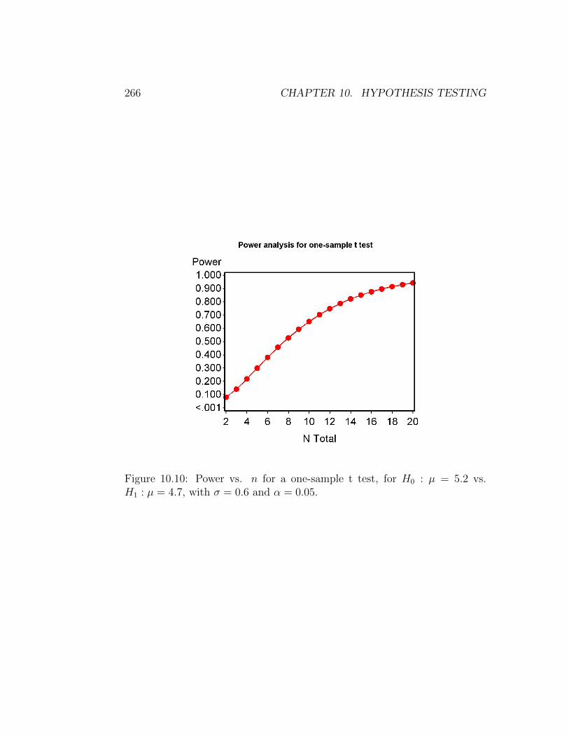
A power analysis can be used to determine an adequate sample size n fora one-sample t test, as well as many other statistical tests. To conduct apower analysis, you need to specify a null and alternative hypothesis, a TypeI error rate α, and have some estimate of the standard deviation σ of thepopulation in question. The analysis then calculates the power for a rangeof n values. The idea is to choose a value of n that gives power closeto 0.8, often regarded as an adequate level of power (Cohen 1988).The power analysis for a one-sample t test involves the same quantity

φ =µ1 − µ0

σ/√n

(10.14)

as for the one-sample Z test, and its power is influenced by the same factors(see Table 10.1). The power calculation involves the non-central t distri-bution with a non-centrality parameter of φ. One subtle difference is thatacceptance and rejection regions for the t test depends on n through the de-grees of freedom, unlike the Z test. Larger values of n lead to smaller valuesof cα,n−1, shrinking the acceptance region and affecting the power calculationin this way.

Returning to the elytra example, suppose we want to test if the lengthof predators reared on an artificial diet differs from wild individuals, whichhave a length of 5.2 mm. This implies H0 : µ = 5.2 mm. For biologicalreasons, we are interested in detecting an decrease or increase in length ofapproximately 10% on the artificial diet, about 0.5 mm. This suggests analternative hypothesis of the form H1 : µ = 5.2− 0.5 = 4.7 mm (or H1 : µ =5.2 + 0.5 = 5.7 mm). How many predators need to be reared on artificialdiet to give a power of at least 0.8? Assume we already have an estimate ofσ from another study, say s = 0.6 mm, and let α = 0.05.

We can use proc power to find the sample size n that gives this power (SASInstitute Inc. 2014). See program and output below. We first specify a one-sample t test using the onesamplemeans option, followed by values for µ underH0 (nullmean = 5.2), σ (stddev = 0.6), and µ under H1 (mean = 4.7). The de-fault value of α is 0.05. We then specify a range of sample sizes (n) for whichwe want the power to be calculated, using the option ntotal = 2 to 20 by 1.This finds the power for n = 2, 3, . . . , 20. The power = . option tells SASsolve for power (there are other possibilities, like finding n for a given powervalue). The option plot x=n generates a low quality plot of power vs. n. We


can generate a better plot by sending the results of proc power to gplot, usingan ods output option. We see that a sample size of n = 14 gives power > 0.8for this scenario. While power increases rapidly for small sample sizes, thereare diminishing returns once the power exceeds about 0.8. In other words,obtaining higher power values requires many more observations.

SAS Program

* One-sample_t_test_power2.sas;

options pageno=1 linesize=80;

goptions reset=all;

title ’Power analysis for one-sample t test’;

proc power;

ods output Plotcontent=plotdata;

onesamplemeans

nullmean = 5.2

stddev = 0.6

mean = 4.7

ntotal = 2 to 20 by 1

power = . ;

plot x=n;

run;

* Plot power vs. sample size in a nicer graph;

proc gplot data=plotall;

plot power*ntotal=1 / vaxis=axis1 haxis=axis1 overlay;

symbol1 i=join v=dot c=red width=3 height=2;

axis1 label=(height=2) value=(height=2) width=3 major=(width=2) minor=none;

run;

quit;


Figure 10.10: Power vs. n for a one-sample t test, for H0 : µ = 5.2 vs.H1 : µ = 4.7, with σ = 0.6 and α = 0.05.


SAS Output

Power analysis for one-sample t test 1

13:34 Wednesday, June 23, 2010

The POWER Procedure

One-sample t Test for Mean

Fixed Scenario Elements

Distribution Normal

Method Exact

Null Mean 5.2

Mean 4.7

Standard Deviation 0.6

Number of Sides 2

Alpha 0.05

Computed Power

N

Index Total Power

1 2 0.081

2 3 0.142

3 4 0.218

4 5 0.300

5 6 0.381

6 7 0.457

7 8 0.528

8 9 0.593

9 10 0.651

10 11 0.703

11 12 0.748

12 13 0.788

13 14 0.822

14 15 0.851

15 16 0.876

16 17 0.897

17 18 0.915

18 19 0.930

19 20 0.942


10.8 One-tailed t test

The tests we have examined so far are known as two-tailed tests. Theyare called this because the test statistic Zs or Ts can detect departures fromH0 : µ = µ0 in both directions, for H1 : µ > µ0 and H1 : µ < µ0, although thealternative for these tests is usually written more compactly as H1 : µ 6= µ0.We will now examine one-tailed tests, which have the same null hypothesisbut the alternative is one direction or the other.

Suppose we are interested in testing H0 : µ = µ0 vs. H1 : µ > µ0. Wecan use the same test statistic as before, namely

Ts =Y − µ0

s/√n. (10.15)

If H1 is true, we would expect to see Y values larger than µ0, and so Tswould be positive. We would reject H0 if Ts was sufficiently positive, withthe acceptance and rejection regions determined as before by controlling theType I error rate. Therefore, if the Type I error rate is α we want to determinea constant c′α,n−1 such that the following statement is true:

P [Ts < c′α,n−1] = 1− α (10.16)

The quantity c′α,n−1 would be chosen using Table T, using the entry for pcorresponding to 1 − α. We would accept H0 if Ts < c′α,n−1 and reject it ifTs ≥ c′α,n−1.

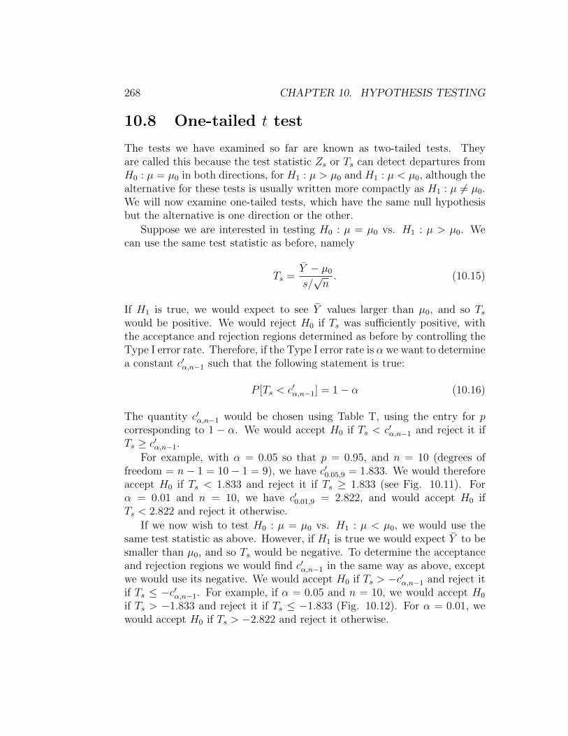
For example, with α = 0.05 so that p = 0.95, and n = 10 (degrees offreedom = n− 1 = 10− 1 = 9), we have c′0.05,9 = 1.833. We would thereforeaccept H0 if Ts < 1.833 and reject it if Ts ≥ 1.833 (see Fig. 10.11). Forα = 0.01 and n = 10, we have c′0.01,9 = 2.822, and would accept H0 ifTs < 2.822 and reject it otherwise.

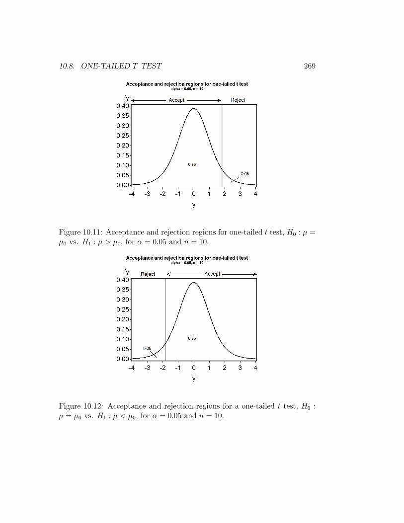
If we now wish to test H0 : µ = µ0 vs. H1 : µ < µ0, we would use thesame test statistic as above. However, if H1 is true we would expect Y to besmaller than µ0, and so Ts would be negative. To determine the acceptanceand rejection regions we would find c′α,n−1 in the same way as above, exceptwe would use its negative. We would accept H0 if Ts > −c′α,n−1 and reject itif Ts ≤ −c′α,n−1. For example, if α = 0.05 and n = 10, we would accept H0

if Ts > −1.833 and reject it if Ts ≤ −1.833 (Fig. 10.12). For α = 0.01, wewould accept H0 if Ts > −2.822 and reject it otherwise.

10.8. ONE-TAILED T TEST 269

Figure 10.11: Acceptance and rejection regions for one-tailed t test, H0 : µ =µ0 vs. H1 : µ > µ0, for α = 0.05 and n = 10.

Figure 10.12: Acceptance and rejection regions for a one-tailed t test, H0 :µ = µ0 vs. H1 : µ < µ0, for α = 0.05 and n = 10.


10.8.1 One-tailed t test - sample calculation

Recall the tilapia example, with Y = 493 g, s2 = 48.2 g2, s = 6.94 g, andn = 10. Suppose we are only interested in detecting diets that produce fishof lower weight than natural food, implying we wish to test H0 : µ = 500 gvs. H1 : µ < 500 g. The test statistic value is again

Ts =Y − µ0

s/√n

=493− 500

6.94/√

10=−7

2.19= −3.196 (10.17)

For α = 0.05 and n− 1 = 10− 1 = 9 degrees of freedom, we have −c′0.05,9 =−1.833. Because Ts = −3.916 < −1.833, we would reject H0 at the α = 0.05level. For α = 0.01, we have −c′0.01,9 = −2.821, and again Ts = −3.196 <−2.821. Thus, we can also reject H0 at the α = 0.01 level. We couldcontinue this process with successively smaller values of α by scanning therow corresponding to 9 degrees of freedom in Table T, but cannot reject H0

for smaller ones. Therefore, we have P < 0.01 for this test.Suppose we had wanted to test H0 : µ = 500 g vs. H1 : µ > 500 g using

the same data and test statistic value, namely Ts = −3.196. The scenariohere could be that we want a commercial diet that actually increases theweight of tilapia over natural food, and are not interested in ones that yieldlower weights. In this case, for α = 0.05 we would not reject H0, becauseTs = −3.196 < 1.833. The test is non-significant, with P > 0.05.

10.8.2 One-tailed t test - SAS demo

Recall the elytra length example, where we tested H0 : µ = 5.2 mm vs.H1 : µ 6= 5.2 mm using SAS. While there is no option for one-tailed tests inproc univariate, we can reinterpret the output and so derive a P value for aone-tailed test.

Suppose we want to test H0 : µ = 5.2 mm vs. H1 : µ < 5.2 mm. Thisimplies we want to test whether predators reared on artificial diet are smallerthan those reared on natural food, which have a length of 5.2 mm. This wouldbe reasonable if we want to detect diets that are deficient in some manner.If H1 were true we would expect to see a negative value of Ts, because Ywould likely be smaller than µ0. This is what occurred in the SAS output,because Y = 4.8 < 5.2 mm and Ts = −1.75:

Student’s t t -1.74574 Pr > |t| 0.1244

10.8. ONE-TAILED T TEST 271

The one-tailed P value in this case is simply half the two-tailed P value,or P (one-tailed) = P (two-tailed)/2= 0.1244/2 = 0.0622. This is becausethe two-tailed test gives the P value for both tails (see Fig. 10.9), but forthis one-tailed test we only need the probability for the left tail of the tdistribution (Fig. 10.12).

Now suppose we want to test H0 : µ = 5.2 mm vs. H1 : µ > 5.2 mm.This implies we want to test whether predators reared on artificial diet arelarger than those reared on natural food. If H1 were true we would expectto see a positive value of Ts, because Y would likely be greater than µ0. Thisis not what occurred in the SAS output, because Y = 4.8 < 5.2 mm andTs = −1.75. The P value should therefore be large in this case, and in factthe one-tailed P value is 1− P (two-tailed) = 1− 0.1244/2 = 0.9378. This isthe probability for the right tail of the t distribution, which is large becauseTs is negative.

We can distill the above procedures to a simple rule that will convertthe SAS two-tailed P value to the appropriate one-tailed one. AssumeH0 : µ = µ0 is the null hypothesis. If the test statistic favors the alter-native hypothesis, then the one-tailed P value is P (two-tailed)/2,otherwise it is 1− P (two-tailed)/2. For example, if we have H1 : µ > µ0

and Ts > 0, the test statistic favors H1 and the P value is P (two-tailed)/2.This procedure also works for tests calculated by hand. You first find the Pvalue for the two-tailed test, then convert it to a one-tailed P value usingthe same rule.

10.8.3 One-tailed tests - a warning

As discussed above, the P value for a one-tailed test may sometimes be halfthe two-tailed P value. This makes it tempting to employ a one-tailed testafter a two-tailed test yields a nonsignificant result. However, the properprocedure is to determine whether a one-tailed alternative hypothesis andtest is appropriate for the situation before conducting the test. For example,artificial diets for insects are unlikely to yield larger insects than naturaldiets, and so it seems reasonable to use an alternative hypothesis of the formH1 : µ < µ0, where µ0 is the size of insects reared on natural foods. Thischoice of an alternative hypothesis can be justified based on prior knowledgeof the system.


10.9 Confidence intervals and hypothesis test-

ing

Confidence intervals are typically used as measures of the accuracy or reli-ability of parameter estimates, but can also be used for hypothesis testing.Why might you do this? There are cases where the statistical software onlyprovides confidence intervals for a parameter, but a test can still be devel-oped using these intervals. Also, a publication may only provide confidenceintervals for a parameter, but the reader can still conduct a test if requiredusing these intervals. Some statisticians argue that this makes confidenceintervals more useful than hypothesis testing, because they also provide in-formation on the magnitude of a population parameter, and how reliably itis estimated (see Yaccoz 1991).

We will now demonstrate how a confidence interval for µ is equivalent toa one-sample t test. Recall that a 100(1− α)% confidence interval for µ hasthe form (

Y − cα,n−1s√n, Y + cα,n−1

s√n

)(10.18)

(see Chapter 9). Suppose that we want to test H0 : µ = µ0. If we accept H0

when this confidence interval includes µ0, and reject it if the interval does notinclude µ0, this is an α level test of H0, equivalent to running a one-samplet test.

To see this connection, note that we would accept H0 if µ0 was inside thisinterval, or

Y − cα,n−1s√n< µ0 < Y + cα,n−1

s√n. (10.19)

Rearranging these inequalities, we see it is equivalent to saying

−cα,n−1 <Y − µ0

s/√n

< cα,n−1, (10.20)

or

−cα,n−1 < Ts < cα,n−1, (10.21)

where Ts is the test statistic for a one-sample t test. We would reject H0

if Ts falls outside this interval. Note that this acceptance region is exactlythe same as for the t test with Type I error rate of α, which is of the form(−cα,n−1, cα,n−1). Thus, the test based on a 100(1− α)% confidence interval

10.10. LIKELIHOOD RATIO TESTS 273

is equivalent to an α level test. In particular, a 95% confidence interval isequivalent to an α = 0.05 test.

Conversely, it is often possible to reverse this process and obtain a confi-dence interval from a statistical test. The procedure is called ‘inverting thetest’ (Bickel & Doksum 1977).

10.10 Likelihood ratio tests

We saw earlier how statisticians use the concept of maximum likelihood to es-timate population parameters (Chapter 8). The maximum likelihood methodbegins by constructing a likelihood function based on the distribution of thedata (Poisson, normal, etc.) and the observed data. We then maximize thelikelihood as a function of the parameters of the distribution (µ, σ2, etc).The values of the parameters that maximize the likelihood are the maximumlikelihood estimates of the parameters. The likelihood function is not a fixedquantity but instead varies with the observed data, so that different datasets yield different estimates of the population parameters. Maximum likeli-hood estimators have desirable statistical properties and in many cases yieldestimators that seem reasonable (like using Y to estimate µ).

Likelihood methods can also be used to develop statistical tests calledlikelihood ratio tests. These tests also have desirable statistical proper-ties and in many cases are identical to classical statistical tests. Likelihoodmethods thus provide a theoretical framework for many statistical problems,including parameter estimation, confidence intervals, and hypothesis testing.The main drawback of these methods is that one must be willing to specifythe distribution of the data, be it Poisson, binomial, normal, or more exoticdistributions.

10.10.1 Example of a likelihood ratio test

We will now develop a likelihood ratio test that leads to the familiar one-sample t test (Mood et al. 1974) . We suppose that the data are normallydistributed and we wish to test H0 : µ = µ0 vs. H1 : µ 6= µ0. A randomsample with n observations has been obtained.

We can think of H0 and H1 as two different statistical models for the data.Under H0, the data are assumed to be normally distributed with µ = µ0, but


can have any value of σ2 because this parameter is left unspecified. UnderH1, the data are permitted to have any value of µ and σ2.

The first step in constructing a likelihood ratio test is to find the maxi-mum likelihood estimates of the parameters for each of these two statisticalmodels. We have already dealt with this problem for the model specified byH1 – this is just maximum likelihood estimation of µ and σ2 for the normaldistribution. The same methods can be used to estimate σ2 under H0, butwe will not go into the details.

This process can be illustrated by plotting the likelihood function as afunction of µ and σ2. To make things more concrete, we show the likelihoodfunction for a data set with three data points (Y1 = 4.5, Y2 = 5.3, andY3 = 5.4). Also shown is a possible null hypothesis for these data, such asH0 : µ = 4.7. See figure below.

The maximum likelihood estimates of µ and σ2 under H1 are the valuesof µ and σ2 found at the peak of the likelihood function. However, themaximum likelihood estimate of σ2 under H0 occurs at a different location.Because µ is fixed at 4.7 under H0, σ2 is only free to vary along the verticalline shown in the figure. The maximum likelihood estimate of σ2 under H0

is the value of σ2 that maximizes the likelihood along this line.

Figure 10.13: Likelihood ratio test for H0 : µ = 4.7

We are now ready to construct the likelihood ratio test statistic. Let LH0

10.10. LIKELIHOOD RATIO TESTS 275

be the maximum height of the likelihood surface under H0, which occurs atthe maximum likelihood estimate of σ2 under H0. Similarly, let let LH1 bethe maximum height under H1, which occurs at the estimates of µ and σ2

under H1. The test statistic λ is just the ratio of these two quantities:

λ =LH0

LH1

. (10.22)

How does this statistic behave? If H0 is true, the peak of the likelihoodfunction will be near the vertical line, and the height of the likelihood functionwill be similar at the two locations. This implies a value of λ ≈ 1 becauseLH0 ≈ LH1 . If H0 is false and H1 true, however, we would expect to seeLH0 < LH1 and so λ < 1. We would therefore reject H0 for sufficiently smallvalues of λ.

More formally, we reject H0 if λ < c and accept H0 otherwise. The valueof c is determined using the Type I error rate α and the distribution of λunder H0.

An alternate form of the test uses −2 ln(λ) rather than λ itself, and rejectsH0 for values of −2 ln(λ) > d, where d is a constant that controls the Type Ierror rate. This form of the test rejects for large values of the test statistic,similar to other tests we have developed. Note that

−2 ln(λ) = 2 ln(LH1)− 2 ln(LH0) (10.23)

by the properties of logarithms, and is a positive quantity. SAS providesvalues of the likelihood function in this format for some statistical procedures,and these can be used to construct likelihood ratio tests.

How is the likelihood ratio test related to a t test? It can be shownmathematically that the value of the test statistic

Ts =Y − µ0

s/√n

(10.24)

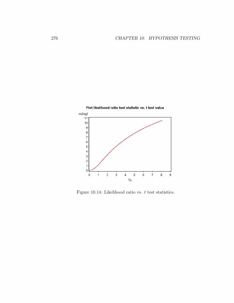
is directly proportional to −2 ln(λ), the likelihood ratio test statistic (Moodet al. 1974). The figure below plots the value of −2 ln(λ) vs. Ts for a scenariomatching our example data set. We observe there is a one-to-one correspon-dence between the two test statistics. When such a correspondence occursbetween two test statistics, the tests are considered to be statistically equiv-alent. We will later see that many statistical tests are in fact likelihood ratiotests. These include tests in analysis of variance, regression, and methodsfor categorical data such as χ2 tests.


Figure 10.14: Likelihood ratio vs. t test statistics.

10.11. REFERENCES 277

10.11 References

Bickel, P. J. & Doksum, K. A. (1977) Mathematical Statistics: Basic Ideasand Selected Topics. Holden-Day, Inc., San Francisco, CA.

Mood, A. M., Graybill, F. A. & Boes, D. C. (1974) Introduction to the Theoryof Statistics. McGraw-Hill, Inc., New York, NY.

SAS Institute Inc. (2014) SAS/STAT 13.2 User’s Guide SAS Institute Inc.,Cary, NC, USA.

Yaccoz, N. G. (1991) Use, overuse, and misuse of significance tests in evolu-tionary biology and ecology. Bulletin of the Ecological Society of America72: 106-111.


10.12 Problems

1. A company that rears beneficial insects produces lacewings (Chrysop-idae: Neuroptera) whose mean length is 10 mm. A new method ofrearing is being tested and the company wants to determine if the newmethod changes lacewing length. A sample of 10 insects is collectedfor the new method, yielding the following lengths:

10.3 14.1 11.5 9.9 12.6 9.7 11.0 9.5 12.4 13.5

(a) Test whether the lacewings produced using the new method havethe same length as before (H0 : µ = 10 vs. H1 : µ 6= 10), usinga two-tailed test and Table T. Provide a P value and discuss thesignificance of the test. Show your calculations.

(b) Suppose the company is only interested in rearing methods thatyield larger lacewing lengths, because bigger is better with benefi-cial insects. Test H0 : µ = 10 vs. H1 : µ > 10. Provide a P valueand discuss the significance of the test.

(c) Use SAS and proc univariate to carry out the same two tests.What are the exact P values for these tests? Attach your SASprogram and printout.

2. A study is done to measure the concentration of a particular chemical(ppm) in drinking water, with samples taken at eight locations. Thesamples were analyzed and the following results obtained:

23 20 24 20 23 24 21 22

(a) Test whether the concentration of the chemical is significantlydifferent from 20 ppm, the level set by the EPA, using a two-tailedtest and Table T. Provide a P value and discuss the significanceof the test. Show your calculations.

(b) The EPA actually requires that the concentration of the chemicalbe equal to or below 20 ppm. Test whether the chemical concen-tration exceeds this level using a one-tailed test and Table T. Inparticular, test H0 : µ = 20 vs. H1 : µ > 20. Provide a P valueand discuss the significance of the test.

10.12. PROBLEMS 279

(c) Use SAS and proc univariate to carry out the same two tests.What are the exact P values for these tests? Attach your SASprogram and printout.

Chapter 10 Hypothesis Testing - · PDF filethis chapter, we examine the ... 250 CHAPTER 10....

Documents

Transcript of Chapter 10 Hypothesis Testing - · PDF filethis chapter, we examine the ... 250 CHAPTER 10....