1

CHAPTER 10 DATA EXPLORATION10.1 Data ExplorationBox 10.1 Data Visualization10.1.1 Descriptive StatisticsBox 10.2 Descriptive Statistics 10.1.2 Graphs10.1.3 Dynamic Graphics10.2 Map-Based Data ManipulationBox 10.3 Geovisualization10.2.1 Data Classification10.2.2 Spatial Aggregation10.2.3 Map Comparison10.3 Attribute Data QueryBox 10.4 Query Methods in ArcGIS10.3.1 SQL (Structured Query Language)10.3.2 Query Expressions10.3.3 Type of Operation10.3.4 Examples of Query Operations10.3.5 Relational Database Query10.4 Spatial Data Query10.4.1 Feature Selection by Cursor10.4.2 Feature Selection by Graphic10.4.3 Feature Selection by Spatial Relationship

Copyright © The McGraw-Hill Companies, Inc. Permission required for reproduction or display.

Box 10.5 Expressions of Spatial Relationship in ArcMap10.4.4 Combining Attribute and Spatial Data Queries10.5 Raster Data Query10.5.1 Query by Cell Value10.5.2 Query by Select FeaturesKey Concepts and TermsReview QuestionsApplications: Data ExplorationTask 1: Select Feature by LocationTask 2: Make Dynamic ChartTask 3: Query Attribute Data from a Joint Attribute TableTask 4: Query Attribute Data from a Relational DatabaseTask 5: Combine Spatial and Attribute Data QueriesTask 6: Query Raster DataChallenge QuestionReferences

2

Data ExplorationCentered on the original data, data exploration allows a

researcher to examine the general trends in the data, to take a close look at data subsets, and to focus on possible relationships between data sets.

Data exploration takes advantage of interactive and dynamically linked visual tools. Maps, graphs, and tables are displayed in multiple windows and dynamically linked so that selecting records from a table will automatically highlight the corresponding features in a graph and a map.

Figure 10.1A line graph.

3

Figure 10.2A histogram.

Figure 10.3A cumulative distribution graph.

4

Figure 10.4A scatterplot plotting % persons 18 years old in 2000 against % population change, 1990–2000. A weak positive relationship, with a correlation coefficient of 0.376, is present between the two variables.

Figure 10.5A bubbleplot showing % population change, 1990–2000, along the x-axis; % persons under 18 years old in 2000 along the y-axis; and state population in 2000 by the bubble size.

5

Figure 10.6A boxplot based on the % population change, 1990–2000, data set.

Figure 10.7Boxplot (a) suggests that the data values follow a normal distribution. Boxplot (b) shows a positively skewed distribution with a higher concentration of data values near the high end. The x’s in (b) may represent outliers, which are more than 1.5 box lengths from the end of the box. Boxplot (c) shows a negatively skewed distribution with a higher concentration of data values near the low end.

6

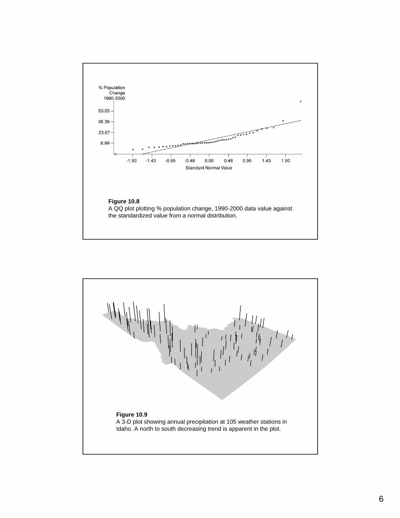
Figure 10.8A QQ plot plotting % population change, 1990-2000 data value against the standardized value from a normal distribution.

Figure 10.9A 3-D plot showing annual precipitation at 105 weather stations in Idaho. A north to south decreasing trend is apparent in the plot.

7

Figure 10.10The scatterplot on the left is dynamically linked to the map on the right. The “brushing” of two data points in the scatterplot highlights the corresponding states (Washington and New Mexico) on the map.

Map-Based Data ManipulationMaps are an important part of GIS operations including data

exploration.

Map-based data manipulation includes data classification, spatial aggregation, and map comparison.

8

Figure 10.11Two classification schemes: above or below the national average (a), and mean and standard deviation (SD) (b).

Figure 10.12Two levels of spatial aggregation: by state (a), and by region (b).

9

Figure 10.13A bivariate map: (1) rate of unemployment in 1997, either above or below the national average, and (2) rate of income change, 1996–1998, either above or below the national average.

Attribute Data Query

Attribute data query retrieves a data subset by working with attribute data.

The selected data subset can be simultaneously examined in the table, displayed in charts, and linked to the highlighted features in the map.

The selected data subset can also be saved for further processing.

10

SQL

SQL (structured query language) is a data query language designed for relational databases.

The basic syntax of SQL includes the following: select <attribute list>, from <relation>, and where <condition>.

ArcGIS has already prepared the keywords in the dialog for querying a local database. Therefore, we only have to enter the where clause (commonly called the query expression) in the dialog box.

Figure 10.14PIN relates the owner and parcel tables and allows use of SQL with both tables.

11

Query ExpressionsQuery expressions consist of Boolean expressions and

connectors.

A simple Boolean expression contains two operands and a logical operator such as Parcel.PIN = ‘P101’ .

Boolean connectors are AND, OR, XOR, and NOT, which are used to connect two or more expressions in a query statement.

Boolean connectors of NOT, AND, and OR are actually keywords used in the operations of Complement, Intersect, and Union on sets in probability.

Figure 10.15The shaded portion represents the complement of data subset A (top), the union of data subsets A and B (middle), and the intersection of A and B (bottom).

12

TABLE 10.1 A Data Set for Query Operation Examples

100N310300Tn45

100N39400Tn44

200N38400Ns13

200Tn47500Ns12

300Tn46500Ns11

AreaSoiltypeCostAreaSoiltypeCost

Type of Operation

Attribute data query begins with a complete data set. A basic query operation is to select a subset. Given a selected data subset, three types of operations can act on it: add more records to the subset, remove records from the subset, and select a smaller subset

13

Figure 10.16Three types of operation may be performed on the subset of 40 records: add more records to the subset (+2), remove records from the subset (-5), or select a smaller subset (20).

Relational Database Query

Relational database query works with a relational database. A query of a table not only selects a data subset in the table butalso selects records related to the subset in other tables.

To query a relational database, we must be familiar with the overall structure of the database, the designation of keys in relating tables, and a data dictionary listing and describing the fields in each table.

14

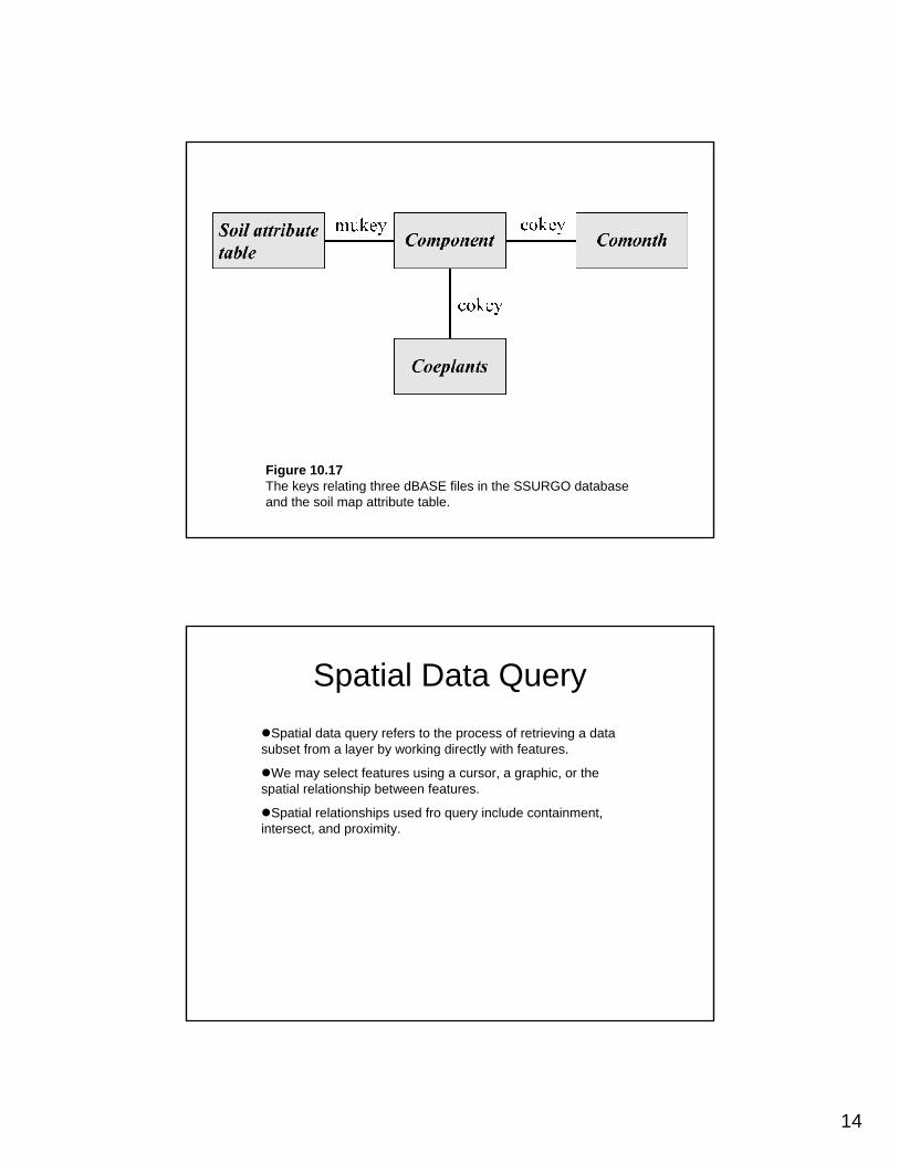
Figure 10.17The keys relating three dBASE files in the SSURGO database and the soil map attribute table.

Spatial Data QuerySpatial data query refers to the process of retrieving a data

subset from a layer by working directly with features.

We may select features using a cursor, a graphic, or the spatial relationship between features.

Spatial relationships used fro query include containment, intersect, and proximity.

15

Figure 10.18Select features by a circle centered at Sun Valley.

Raster Data QueryRaster data can be queried by cell value and select features.

16

Figure 10.19Raster data query: slope = 2 and aspect = 1. Selected cells are coded 1 and others 0 in the output raster.

gnuplothttp://www.gnuplot.info/U.S. Census Bureauhttp://www.census.gov/