CHAPTER 10 Comparing Two Populations or Groups€¦ · · 2018-04-04PERFORM a significance test...
22
The Practice of Statistics, 5th Edition Starnes, Tabor, Yates, Moore Bedford Freeman Worth Publishers CHAPTER 10 Comparing Two Populations or Groups 10.1 Comparing Two Proportions
Transcript of CHAPTER 10 Comparing Two Populations or Groups€¦ · · 2018-04-04PERFORM a significance test...

The Practice of Statistics, 5th Edition
Starnes, Tabor, Yates, Moore
Bedford Freeman Worth Publishers
CHAPTER 10Comparing Two Populations or Groups
10.1
Comparing Two Proportions
Learning Objectives
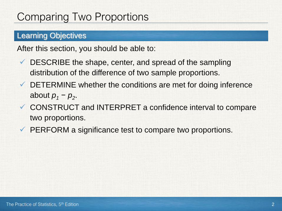
After this section, you should be able to:
The Practice of Statistics, 5th Edition 2
✓ DESCRIBE the shape, center, and spread of the sampling
distribution of the difference of two sample proportions.
✓ DETERMINE whether the conditions are met for doing inference
about p1 − p2.
✓ CONSTRUCT and INTERPRET a confidence interval to compare
two proportions.
✓ PERFORM a significance test to compare two proportions.
Comparing Two Proportions

The Practice of Statistics, 5th Edition 3
Introduction
Suppose we want to compare the proportions of individuals with a
certain characteristic in Population 1 and Population 2. Let’s call these
parameters of interest p1 and p2. The ideal strategy is to take a
separate random sample from each population and to compare the
sample proportions with that characteristic.
What if we want to compare the effectiveness of Treatment 1 and
Treatment 2 in a completely randomized experiment? This time, the
parameters p1 and p2 that we want to compare are the true proportions
of successful outcomes for each treatment. We use the proportions of
successes in the two treatment groups to make the comparison.
The Practice of Statistics, 5th Edition 4
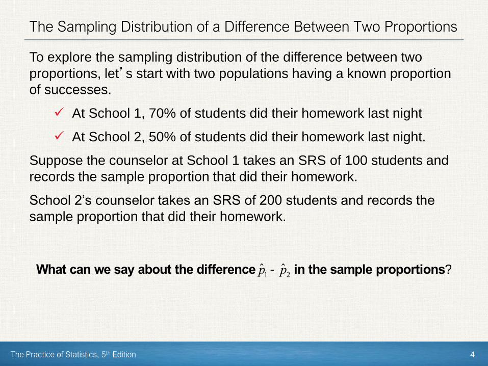
The Sampling Distribution of a Difference Between Two Proportions
To explore the sampling distribution of the difference between two
proportions, let’s start with two populations having a known proportion
of successes.
✓ At School 1, 70% of students did their homework last night
✓ At School 2, 50% of students did their homework last night.
Suppose the counselor at School 1 takes an SRS of 100 students and
records the sample proportion that did their homework.
School 2’s counselor takes an SRS of 200 students and records the
sample proportion that did their homework.
What can we say about the difference ˆ p 1 - ˆ p 2 in the sample proportions?
The Practice of Statistics, 5th Edition 5
The Sampling Distribution of a Difference Between Two Proportions
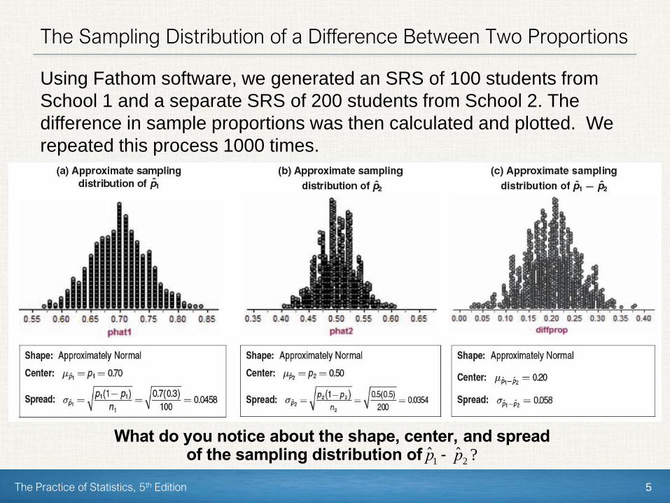
Using Fathom software, we generated an SRS of 100 students from
School 1 and a separate SRS of 200 students from School 2. The
difference in sample proportions was then calculated and plotted. We
repeated this process 1000 times.
What do you notice about the shape, center, and spreadof the sampling distribution of ˆ p 1 - ˆ p 2 ?

The Practice of Statistics, 5th Edition 6
The Sampling Distribution of the Difference Between Sample Proportions
Choose an SRS of size n1 from Population 1 with proportion of
successes p1 and an independent SRS of size n2 from Population 2
with proportion of successes p2.
The Sampling Distribution of a Difference Between Two Proportions
Both ˆ p 1 and ˆ p 2 are random variables. The statistic ˆ p 1 - ˆ p 2 is the differenceof these two random variables. In Chapter 6, we learned that for any two independent random variables X and Y,
mX -Y = mX - mY and s X -Y
2 = sX
2 + sY
2
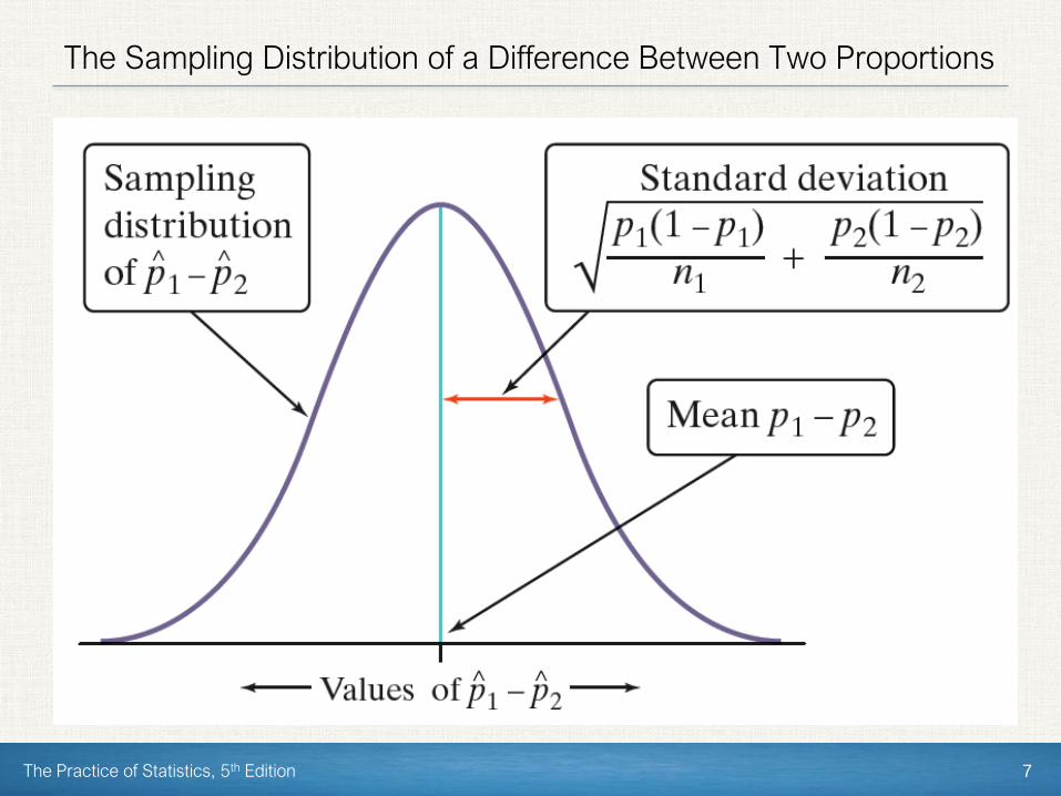
Shape When n1p1, n1(1- p1), n2 p2 and n2(1- p2) are all at least 10, the
sampling distribution of ˆ p 1 - ˆ p 2 is approximately Normal.
Spread The standard deviation of the sampling distribution of ˆ p 1 - ˆ p 2 is
p1(1- p1)
n1
+p2(1- p2)
n2
as long as each sample is no more than 10% of its population (10% condition).
The Practice of Statistics, 5th Edition 7
The Sampling Distribution of a Difference Between Two Proportions
The Practice of Statistics, 5th Edition 8
The Sampling Distribution of a Difference Between Two Proportions
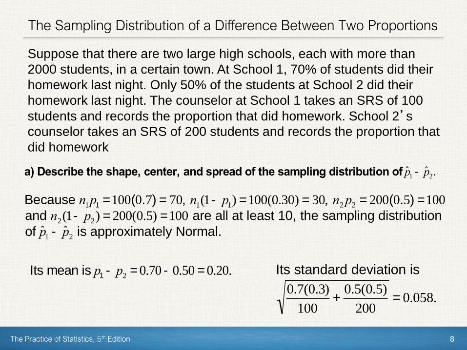
Suppose that there are two large high schools, each with more than
2000 students, in a certain town. At School 1, 70% of students did their
homework last night. Only 50% of the students at School 2 did their
homework last night. The counselor at School 1 takes an SRS of 100
students and records the proportion that did homework. School 2’s
counselor takes an SRS of 200 students and records the proportion that
did homework
a) Describe the shape, center, and spread of the sampling distribution of ˆ p 1 - ˆ p 2.
Because n1p1 =100(0.7) = 70, n1(1- p1) =100(0.30) = 30, n2 p2 = 200(0.5) =100
and n2(1- p2) = 200(0.5) =100 are all at least 10, the sampling distribution
of ˆ p 1 - ˆ p 2 is approximately Normal.
Its mean is p1 - p2 = 0.70 -0.50 = 0.20.
Its standard deviation is
0.7(0.3)
100+
0.5(0.5)
200= 0.058.

The Practice of Statistics, 5th Edition 9
American made cars
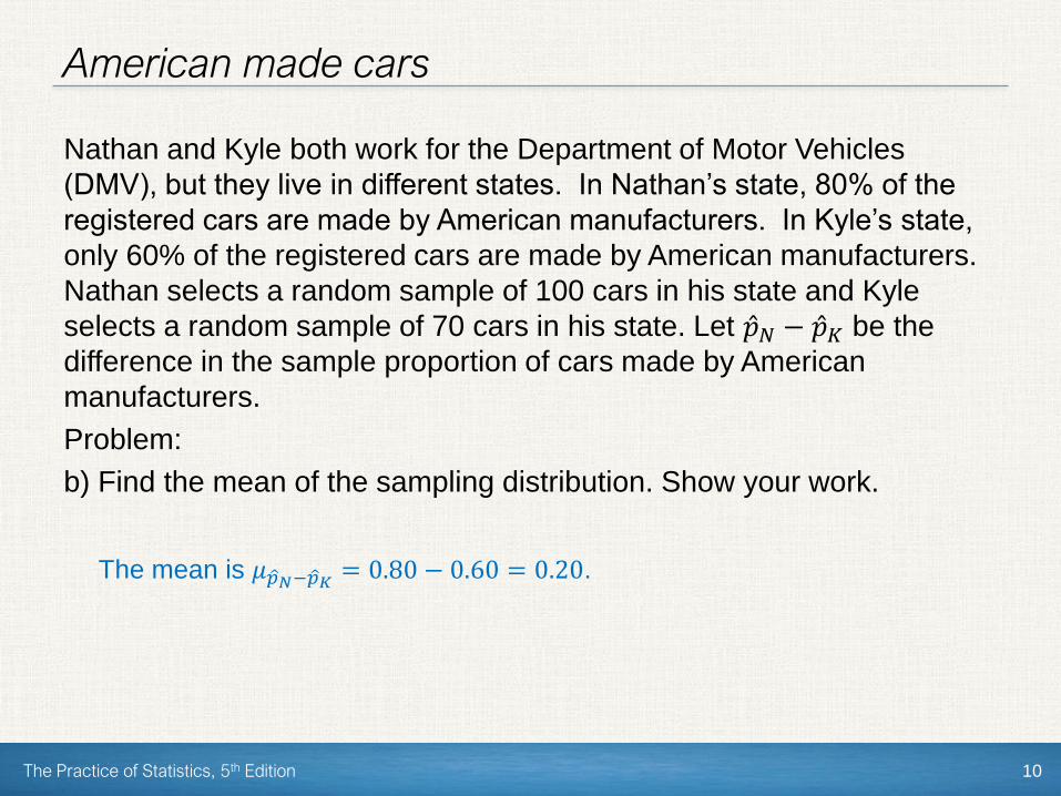
Nathan and Kyle both work for the Department of Motor Vehicles
(DMV), but they live in different states. In Nathan’s state, 80% of the
registered cars are made by American manufacturers. In Kyle’s state,
only 60% of the registered cars are made by American manufacturers.
Nathan selects a random sample of 100 cars in his state and Kyle
selects a random sample of 70 cars in his state. Let Ƹ𝑝𝑁 − Ƹ𝑝𝐾 be the
difference in the sample proportion of cars made by American
manufacturers.
Problem:
a)What is the shape of the sampling distribution of Ƹ𝑝𝑁 − Ƹ𝑝𝐾? Why?
Because 100(0.80) = 80, 100(1 – 0.80) = 20, 70(0.60) = 42, and 70(1 –
0.60) = 28 are all ≥ 10, the sampling distribution of Ƹ𝑝𝑁 − Ƹ𝑝𝐾 is
approximately Normal.
The Practice of Statistics, 5th Edition 10
American made cars
Nathan and Kyle both work for the Department of Motor Vehicles
(DMV), but they live in different states. In Nathan’s state, 80% of the
registered cars are made by American manufacturers. In Kyle’s state,
only 60% of the registered cars are made by American manufacturers.
Nathan selects a random sample of 100 cars in his state and Kyle
selects a random sample of 70 cars in his state. Let Ƹ𝑝𝑁 − Ƹ𝑝𝐾 be the
difference in the sample proportion of cars made by American
manufacturers.
Problem:
b) Find the mean of the sampling distribution. Show your work.
The mean is 𝜇 ො𝑝𝑁− ො𝑝𝐾 = 0.80 − 0.60 = 0.20.

The Practice of Statistics, 5th Edition 11
American made cars
Nathan and Kyle both work for the Department of Motor Vehicles
(DMV), but they live in different states. In Nathan’s state, 80% of the
registered cars are made by American manufacturers. In Kyle’s state,
only 60% of the registered cars are made by American manufacturers.
Nathan selects a random sample of 100 cars in his state and Kyle
selects a random sample of 70 cars in his state. Let Ƹ𝑝𝑁 − Ƹ𝑝𝐾 be the
difference in the sample proportion of cars made by American
manufacturers.
Problem:
c) Find the standard deviation of the sampling distribution. Show your
work.
Because there are at least 10(100) = 1000 cars in Nathan’s state and at
least 10(70) = 700 cars in Kyle’s state, the standard deviation is
𝜎 ො𝑝𝑁− ො𝑝𝐾 =0.80(0.20)
100+0.60(0.40)
70= 0.0709
The Practice of Statistics, 5th Edition 12
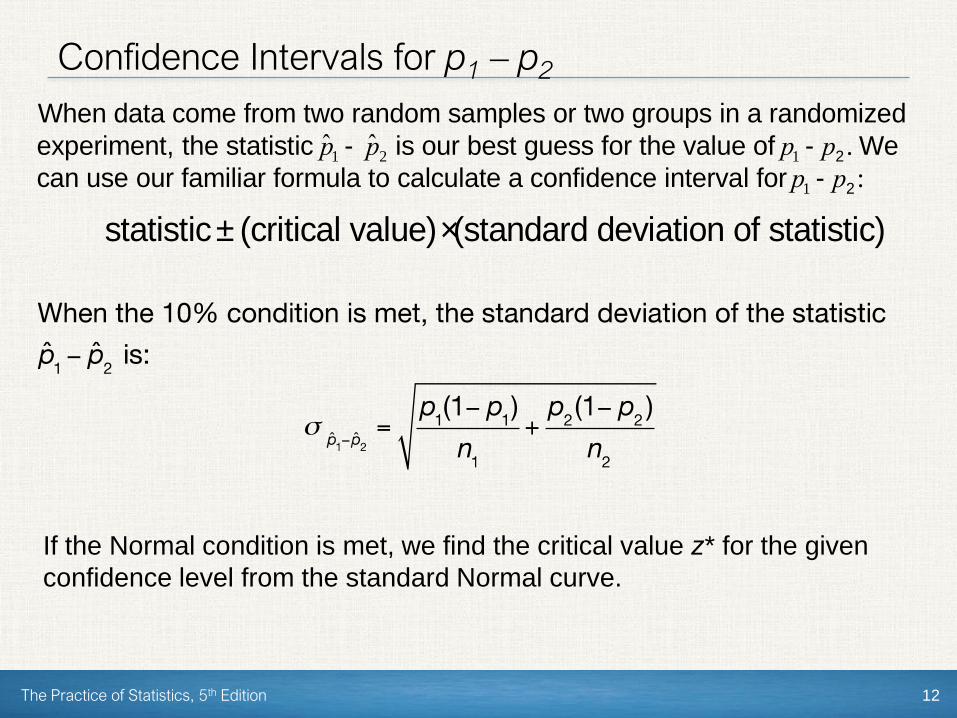
Confidence Intervals for p1 – p2
When data come from two random samples or two groups in a randomized
experiment, the statistic ˆ p 1 - ˆ p 2 is our best guess for the value of p1 -p2 . We
can use our familiar formula to calculate a confidence interval for p1 -p2:
statistic± (critical value) × (standard deviation of statistic)
If the Normal condition is met, we find the critical value z* for the given
confidence level from the standard Normal curve.
The Practice of Statistics, 5th Edition 13
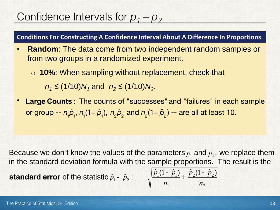
Confidence Intervals for p1 – p2
Conditions For Constructing A Confidence Interval About A Difference In Proportions
• Random: The data come from two independent random samples or
from two groups in a randomized experiment.
o 10%: When sampling without replacement, check that
n1 ≤ (1/10)N1 and n2 ≤ (1/10)N2.
•
Because we don't know the values of the parameters p1 and p2, we replace them
in the standard deviation formula with the sample proportions. The result is the
standard error of the statistic ˆ p 1 - ˆ p 2 : ˆ p 1(1- ˆ p 1)
n1
+ˆ p 2(1- ˆ p 2)
n2
The Practice of Statistics, 5th Edition 14
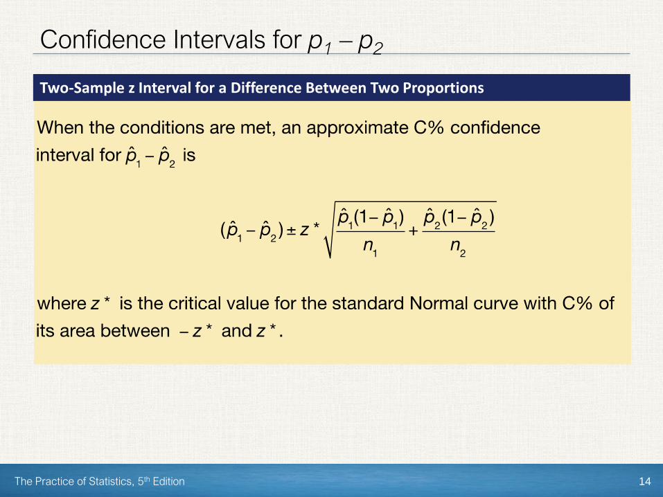
Confidence Intervals for p1 – p2
Two-Sample z Interval for a Difference Between Two Proportions
The Practice of Statistics, 5th Edition 15
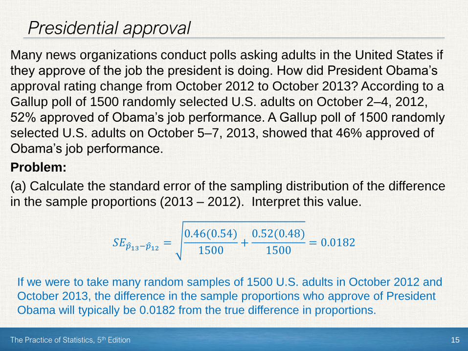
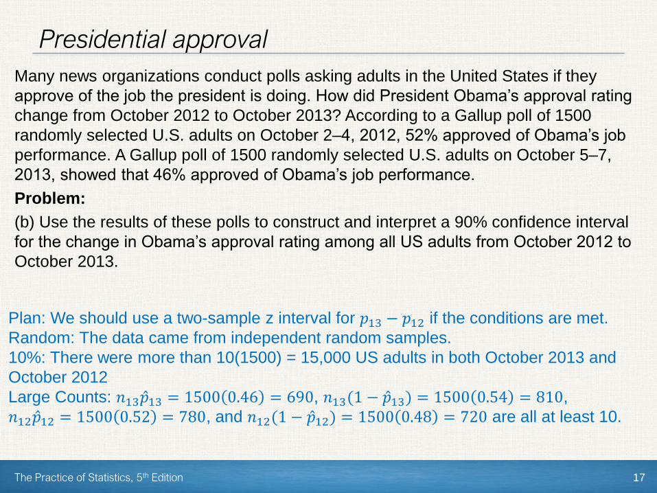
Presidential approval
Many news organizations conduct polls asking adults in the United States if
they approve of the job the president is doing. How did President Obama’s
approval rating change from October 2012 to October 2013? According to a
Gallup poll of 1500 randomly selected U.S. adults on October 2–4, 2012,
52% approved of Obama’s job performance. A Gallup poll of 1500 randomly
selected U.S. adults on October 5–7, 2013, showed that 46% approved of
Obama’s job performance.
Problem:
(a) Calculate the standard error of the sampling distribution of the difference
in the sample proportions (2013 – 2012). Interpret this value.
𝑆𝐸 ො𝑝13− ො𝑝12 =0.46(0.54)
1500+0.52(0.48)
1500= 0.0182
If we were to take many random samples of 1500 U.S. adults in October 2012 and
October 2013, the difference in the sample proportions who approve of President
Obama will typically be 0.0182 from the true difference in proportions.

The Practice of Statistics, 5th Edition 16
Presidential approval
Many news organizations conduct polls asking adults in the United States if they
approve of the job the president is doing. How did President Obama’s approval rating
change from October 2012 to October 2013? According to a Gallup poll of 1500
randomly selected U.S. adults on October 2–4, 2012, 52% approved of Obama’s job
performance. A Gallup poll of 1500 randomly selected U.S. adults on October 5–7,
2013, showed that 46% approved of Obama’s job performance.
Problem:
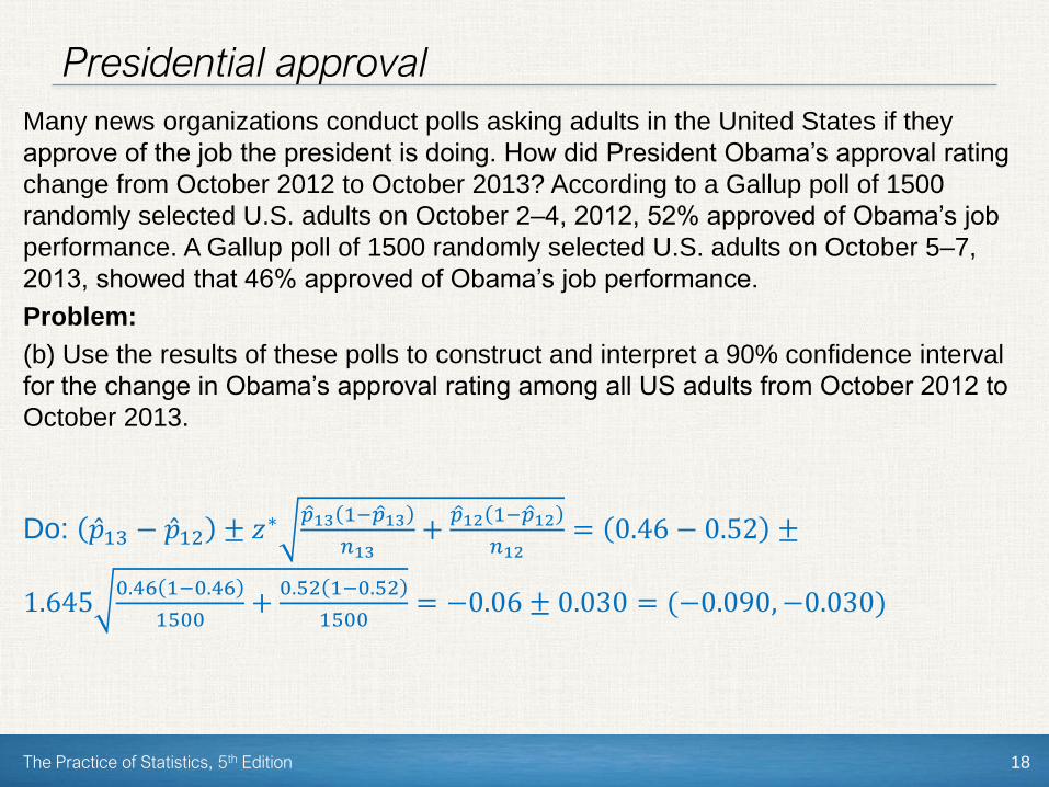
(b) Use the results of these polls to construct and interpret a 90% confidence interval
for the change in Obama’s approval rating among all US adults from October 2012 to
October 2013.
State: We want to estimate 𝑝13 − 𝑝12 at the 90% confidence level where
𝑝13 is the true proportion of al US adults who approved of President Obama’s job
performance in October 2013 and
𝑝12 is the true proportion of all US adults who approved of President Obama’s job
performance in October 2012.
The Practice of Statistics, 5th Edition 17
Presidential approval
Many news organizations conduct polls asking adults in the United States if they
approve of the job the president is doing. How did President Obama’s approval rating
change from October 2012 to October 2013? According to a Gallup poll of 1500
randomly selected U.S. adults on October 2–4, 2012, 52% approved of Obama’s job
performance. A Gallup poll of 1500 randomly selected U.S. adults on October 5–7,
2013, showed that 46% approved of Obama’s job performance.
Problem:
(b) Use the results of these polls to construct and interpret a 90% confidence interval
for the change in Obama’s approval rating among all US adults from October 2012 to
October 2013.
Plan: We should use a two-sample z interval for 𝑝13 − 𝑝12 if the conditions are met.
Random: The data came from independent random samples.
10%: There were more than 10(1500) = 15,000 US adults in both October 2013 and
October 2012
Large Counts: 𝑛13 Ƹ𝑝13 = 1500 0.46 = 690, 𝑛13(1 − Ƹ𝑝13) = 1500 0.54 = 810,
𝑛12 Ƹ𝑝12 = 1500 0.52 = 780, and 𝑛12(1 − Ƹ𝑝12) = 1500 0.48 = 720 are all at least 10.
The Practice of Statistics, 5th Edition 18
Presidential approval
Many news organizations conduct polls asking adults in the United States if they
approve of the job the president is doing. How did President Obama’s approval rating
change from October 2012 to October 2013? According to a Gallup poll of 1500
randomly selected U.S. adults on October 2–4, 2012, 52% approved of Obama’s job
performance. A Gallup poll of 1500 randomly selected U.S. adults on October 5–7,
2013, showed that 46% approved of Obama’s job performance.
Problem:
(b) Use the results of these polls to construct and interpret a 90% confidence interval
for the change in Obama’s approval rating among all US adults from October 2012 to
October 2013.
Do: Ƹ𝑝13 − Ƹ𝑝12 ± 𝑧∗ො𝑝13 1− ො𝑝13
𝑛13+
ො𝑝12 1− ො𝑝12
𝑛12= 0.46 − 0.52 ±
1.6450.46 1−0.46
1500+
0.52 1−0.52
1500= −0.06 ± 0.030 = (−0.090,−0.030)

The Practice of Statistics, 5th Edition 19
Presidential approval
Many news organizations conduct polls asking adults in the United States if they
approve of the job the president is doing. How did President Obama’s approval rating
change from October 2012 to October 2013? According to a Gallup poll of 1500
randomly selected U.S. adults on October 2–4, 2012, 52% approved of Obama’s job
performance. A Gallup poll of 1500 randomly selected U.S. adults on October 5–7,
2013, showed that 46% approved of Obama’s job performance.
Problem:
(b) Use the results of these polls to construct and interpret a 90% confidence interval
for the change in Obama’s approval rating among all US adults from October 2012 to
October 2013.
Conclude: We are 90% confident that the interval from −0.090 to –0.030
captures the true change in the proportion of U.S. adults who approve of
President Obama’s job performance from October 2012 to October 2013.
The Practice of Statistics, 5th Edition 20
Presidential approval
Many news organizations conduct polls asking adults in the United States if they
approve of the job the president is doing. How did President Obama’s approval rating
change from October 2012 to October 2013? According to a Gallup poll of 1500
randomly selected U.S. adults on October 2–4, 2012, 52% approved of Obama’s job
performance. A Gallup poll of 1500 randomly selected U.S. adults on October 5–7,
2013, showed that 46% approved of Obama’s job performance.
Problem:
(c) Based on your interval, is there convincing evidence that Obama’s job approval
rating has changed?
Because 0 is not included in the interval, we have convincing evidence that
President Obama’s approval rating has changed from October 2012 to
October 2013.
Section Summary
In this section, we learned how to…
The Practice of Statistics, 5th Edition 21
✓ DESCRIBE the shape, center, and spread of the sampling distribution
of the difference of two sample proportions.
✓ DETERMINE whether the conditions are met for doing inference
about p1 − p2.
✓ CONSTRUCT and INTERPRET a confidence interval to compare two
proportions.
Comparing Two Proportions

The Practice of Statistics, 5th Edition 22
PAGE 629
2, 6, 10Homework