Copyright © 2010 by the McGraw-Hill Companies, Inc. All rights reserved.McGraw-Hill/Irwin

Managerial Economics & Business Strategy

Chapter 1:The Fundamentals of

Managerial Economics

1-2

OverviewI. IntroductionII. The Economics of Effective Management

– Identify Goals and Constraints– Recognize the Role of Profits– Five Forces Model– Understand Incentives – Understand Markets– Recognize the Time Value of Money– Use Marginal Analysis

1-3

Managerial Economics� Manager

– A person who directs resources to achieve a stated goal.

� Economics– The science of making decisions in the

presence of scare resources.

� Managerial Economics– The study of how to direct scarce resources in

the way that most efficiently achieves a managerial goal.

1-4

Identify Goals and Constraints

� Sound decision making involves having well-defined goals.– Leads to making the “right” decisions.

� In striking to achieve a goal, we often face constraints.– Constraints are an artifact of scarcity.

1-5

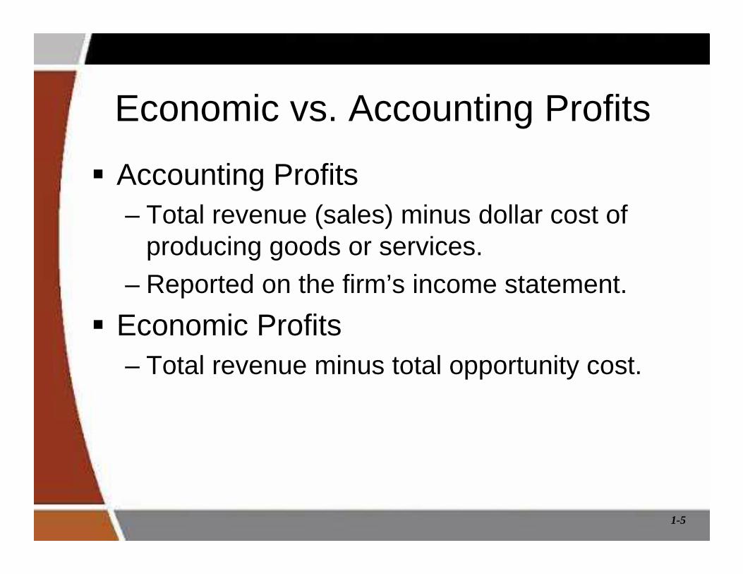
Economic vs. Accounting Profits

� Accounting Profits– Total revenue (sales) minus dollar cost of

producing goods or services.– Reported on the firm’s income statement.

� Economic Profits– Total revenue minus total opportunity cost.

1-6

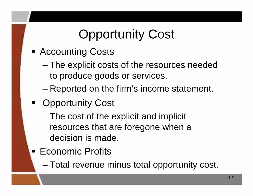
Opportunity Cost� Accounting Costs

– The explicit costs of the resources needed to produce goods or services.

– Reported on the firm’s income statement.

� Opportunity Cost– The cost of the explicit and implicit

resources that are foregone when a decision is made.

� Economic Profits– Total revenue minus total opportunity cost.

1-7

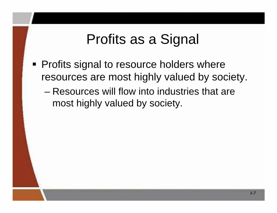
Profits as a Signal

� Profits signal to resource holders where resources are most highly valued by society.– Resources will flow into industries that are

most highly valued by society.

1-8

The Five Forces Framework

Sustainable IndustryProfits

Power ofInput Suppliers

•Supplier Concentration•Price/Productivity of Alternative Inputs•Relationship-Specific Investments•Supplier Switching Costs•Government Restraints

Power ofBuyers

•Buyer Concentration•Price/Value of Substitute Products or Services•Relationship-Specific Investments•Customer Switching Costs•Government Restraints

Entry•Entry Costs•Speed of Adjustment•Sunk Costs•Economies of Scale

•Network Effects•Reputation•Switching Costs•Government Restraints

Substitutes & Complements•Price/Value of Surrogate Products or Services•Price/Value of Complementary Products or Services

•Network Effects•Government Restraints

Industry Rivalry•Switching Costs•Timing of Decisions•Information•Government Restraints

•Concentration•Price, Quantity, Quality, or Service Competition•Degree of Differentiation

1-9

Understanding Firms’ Incentives� Incentives play an important role within the

firm.� Incentives determine:

– How resources are utilized.

– How hard individuals work.

� Managers must understand the role incentives play in the organization.

� Constructing proper incentives will enhance productivity and profitability.

1-10

Market Interactions� Consumer-Producer Rivalry

– Consumers attempt to locate low prices, while producers attempt to charge high prices.

� Consumer-Consumer Rivalry– Scarcity of goods reduces consumers’ negotiating

power as they compete for the right to those goods.

� Producer-Producer Rivalry– Scarcity of consumers causes producers to compete

with one another for the right to service customers.

� The Role of Government– Disciplines the market process.

1-11

The Time Value of Money� Present value (PV) of a future value (FV)

lump-sum amount to be received at the end of “n” periods in the future when the per-period interest rate is “i”:

( )PVFV

i n=+1

• Examples:� Lotto winner choosing between a single lump-sum payout of $104

million or $198 million over 25 years.

� Determining damages in a patent infringement case.

1-12

Present Value vs. Future Value

� The present value (PV) reflects the difference between the future value and the opportunity cost of waiting (OCW).

� Succinctly,PV = FV – OCW

� If i = 0, note PV = FV.� As i increases, the higher is the OCW and the

lower the PV.

1-13

Present Value of a Series

� Present value of a stream of future amounts (FVt) received at the end of each period for “n” periods:

� Equivalently,

( )∑= +

=n

tt

t

i

FVPV

1 1

( ) ( ) ( )PVFV

i

FV

i

FV

in

n=+

++

+ ++

11

221 1 1

...

1-14

Net Present Value

� Suppose a manager can purchase a stream of future receipts (FVt ) by spending “C0”dollars today. The NPV of such a decision is

( ) ( ) ( )NPVFV

i

FV

i

FV

iCn

n=+

++

+ ++

−11

22 01 1 1

...

Decision Rule:If NPV < 0: Reject project

NPV > 0: Accept project

1-15

Present Value of a Perpetuity� An asset that perpetually generates a

stream of cash flows (CFi) at the end of each period is called a perpetuity.

� The present value (PV) of a perpetuity of cash flows paying the same amount (CF = CF1 = CF2 = …) at the end of each period is

( ) ( ) ( )

i

CF

i

CF

i

CF

i

CFPVPerpetuity

=

++

++

++

= ...111 32

1-16

Firm Valuation and Profit Maximization

� The value of a firm equals the present value of current and future profits (cash flows).

� A common assumption among economist is that it is the firm’s goal to maximization profits.– This means the present value of current and future

profits, so the firm is maximizing its value.

( ) ( ) ( )∑∞

= +=+

++

++=

1

210

1...

11 tt

tFirm

iiiPV

ππππ

1-17

Firm Valuation With Profit Growth� If profits grow at a constant rate (g < i) and

current period profits are πο, before and after dividends are:

� Provided that g < i.– That is, the growth rate in profits is less than

the interest rate and both remain constant.

0

0

1 before current profits have been paid out as dividends;

1 immediately after current profits are paid out as dividends.

Firm

Ex DividendFirm

iPV

i g

gPV

i g

π

π−

+=−

+=−

1-18

� Control Variable Examples:– Output– Price

– Product Quality– Advertising

– R&D

� Basic Managerial Question: How much of the control variable should be used to maximize net benefits?

Marginal (Incremental) Analysis

1-19

Net Benefits

� Net Benefits = Total Benefits - Total Costs� Profits = Revenue - Costs

1-20

Marginal Benefit (MB)

� Change in total benefits arising from a change in the control variable, Q:

� Slope (calculus derivative) of the total benefit curve.

Q

BMB

∆∆=

1-21

Marginal Cost (MC)

� Change in total costs arising from a change in the control variable, Q:

� Slope (calculus derivative) of the total cost curve.

Q

CMC

∆∆=

1-22

Marginal Principle

� To maximize net benefits, the managerial control variable should be increased up to the point where MB = MC.

� MB > MC means the last unit of the control variable increased benefits more than it increased costs.

� MB < MC means the last unit of the control variable increased costs more than it increased benefits.

1-23

The Geometry of Optimization: Total Benefit and Cost

Q

Total Benefits& Total Costs

Benefits

Costs

Q*

B

CSlope = MC

Slope =MB

1-24

The Geometry of Optimization: Net Benefits

Q

Net Benefits

Maximum net benefits

Q*

Slope = MNB

1-25

Conclusion

� Make sure you include all costs and benefits when making decisions (opportunity cost).

� When decisions span time, make sure you are comparing apples to apples (PV analysis).

� Optimal economic decisions are made at the margin (marginal analysis).