Chapter 1 Sensor Defects in Digital Image...

Chapter 1

Sensor Defects in Digital Image Forensic

Jessica Fridrich

Just as human fingerprints or skin blemishes can be used for forensic pur-poses, imperfections of digital imaging sensors can serve as unique identifiersin numerous forensic applications, such as matching an image to a specificcamera, revealing malicious image manipulation and processing, and deter-mining an approximate age of a digital photograph. There exist several dif-ferent types of defects that are of interest to the forensic analyst caused byimperfections in manufacturing, physical processes occurring inside the cam-era, and by environmental factors. This chapter begins with analyzing pixeldefects, while pointing out their forensic potential. Then, specific problemsare formulated as tasks involving detection or matching of defects and noisepatterns. Practical algorithms for these tasks are developed within the frame-work of parameter estimation and signal detection theory. The performanceof the algorithms is demonstrated on real-world examples.

1.1 Introduction

In the heart of every electronic device capable of taking digital pictures is animaging sensor. There exist two types of sensors – CCD (Charge-Coupled De-vice) and CMOS (Complementary Metal-Oxide Semiconductor). Both sen-sors consist of a large number of photo detectors commonly called pixels.Pixels are made of silicon and capture light by converting photons into elec-trons using the photoelectric effect [30, 27]. The charge accumulated at everypixel is transferred out of the sensor, amplified, and then run through an ADconverter that converts it to a digital signal. The digitized signal is furtherprocessed before the data is stored as an electronic file (JPEG, TIFF, etc.) onthe camera storage device. The pixels are several microns across and have arectangular shape. In theory, the amount of electrons (charge) outputted bya pixel should depend solely on the intensity of the incident light. In reality,

1

2 Jessica Fridrich

however, there are many factors that introduce both systematic and randomdeviations. It is exactly these fluctuations that find important applicationsin forensic analysis.

We will be interested primarily in systematic variations in pixel responsethat manifest themselves in a consistent manner in all images because ran-dom fluctuations that change independently from scene to scene would notbe particularly useful. In the next section, we describe several types of suchsystematic sensor defects and how they affect the output of a sensor. By doingso, we arrive at a model of sensor output that will be useful later for deriv-ing estimators of parameters that describe the defects and for constructingdefect detectors. In Section 1.3, we introduce the concept of sensor finger-print and derive a procedure using which the fingerprint can be estimatedfrom images taken by the camera. The tasks of camera identification, devicelinking, and forgery detection can be approached by testing the presence ofsensor fingerprint in images. This is the subject of Sections 1.4, 1.4.1, and1.4.4. The methods are tested on real images in Section 1.5. In Section 1.6,we develop methods that can address counter-forensic activities of the typewhen an adversary estimates a camera fingerprint and then adds it to animage from a different camera to frame an innocent victim. The presence orabsence of defects can also provide temporal information for estimating anapproximate age of digital photographs. This so-called temporal forensics isthe subject of Section 1.7. The chapter is summarized in Section 1.8.

1.1.1 Notation

Everywhere in this chapter, boldface font will denote vectors (or matrices) oflength specified in the text, e.g., X and Y are vectors of length m × n andX(i) denotes the ith component of X. Sometimes, we will index the pixels inan image using a two-dimensional index formed by the row and column index.Unless mentioned otherwise, all operations among vectors or matrices, suchas product, ratio, raising to a power, etc., are elementwise. The Euclideandot product of vectors is denoted as X ·Y with ‖X‖ =

√X ·X being the L2

(Euclidean) norm of X. Denoting the sample mean with a bar, the normalizedcorrelation is

corr(X, Y) =(X−X) · (Y −Y)∥

∥X−X∥

∥

∥

∥Y−Y∥

∥

. (1.1)

For a logical statement P , we also make use of the Iverson bracket definedas [P ] = 1 when P is true and [P ] = 0 when P is false.

1 Sensor Defects in Digital Image Forensic 3

1.2 Imaging sensors and their defects

In this section, we explain two types of systematic defects – the photo-response non-uniformity and dark current – that are useful for several im-portant forensic tasks, including camera identification and forgery detection.Then, we formulate a model of pixel output that will be used in the rest ofthis chapter to build all necessary mathematical tools for the forensic analyst.

1.2.1 Photo-response non-uniformity

The charge generated in a pixel depends on the physical dimensions of thepixel photosensitive area and on the homogeneity of silicon. The pixels’ phys-ical dimensions slightly vary due to imperfections in the manufacturing pro-cess. Also, the inhomogeneity naturally present in silicon contributes to vari-ations in quantum efficiency among pixels (the ability to convert photons toelectrons). The variations in quantum efficiency among pixels can be capturedwith a matrix K ∈ R

m×n of the same dimensions as the sensor. When animaging sensor is illuminated with light intensity I ∈ R

m×n, in the absence ofother noise sources or imperfections, the sensor would register a noisy sceneI + IK instead. (We remind that the product IK is an element-wise productof matrices) The term IK is usually referred to as the photo-response non-uniformity or PRNU. A large value of K leads to a point defect called “pixelwith abnormal sensitivity.”

One can say that the scene I is overlaid with a “noise pattern” IK, whichis essentially the matrix K modulated by the scene I. Note that the energyof this noise pattern depends on the light intensity – it is larger for brightimages and smaller in pictures of mostly dark scenes.

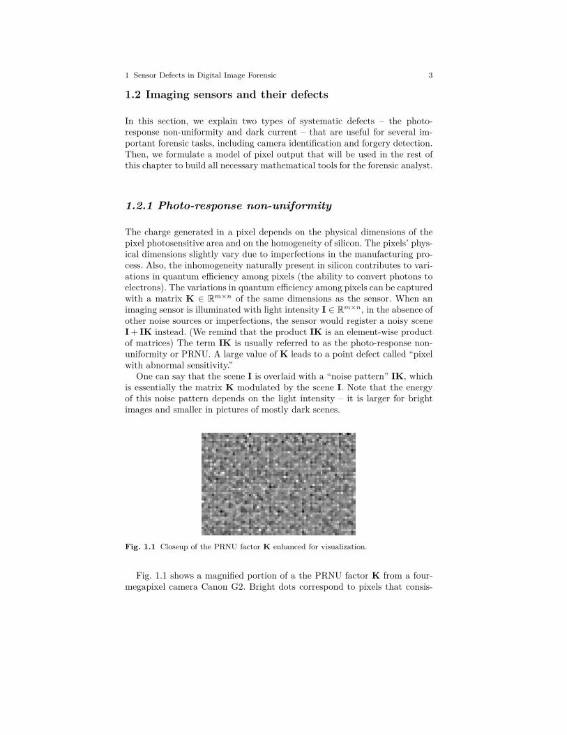
Fig. 1.1 Closeup of the PRNU factor K enhanced for visualization.

Fig. 1.1 shows a magnified portion of a the PRNU factor K from a four-megapixel camera Canon G2. Bright dots correspond to pixels that consis-

4 Jessica Fridrich

tently generate more electrons, while dark dots mark pixels whose responseis consistently lower. To give the reader a sense of how weak the PRNU sig-nal IK typically is, for a picture of a uniform background I with averagegrayscale in the middle of the dynamic range (grayscale I = 128 for an 8-bitimage), the average energy of I(i)K(i) over all pixels i is 0.5, which can alsobe formulated as SNR of 51 dB. The energy of the PRNU strongly variesamong camera models.

In Section 1.3, it is shown how the PRNU factor K can be used as a sensor“fingerprint” for a variety of forensic tasks.

1.2.2 Dark current

Even when a pixel is not exposed to light during picture taking, it contains asmall number of free electrons due to thermal effects. Their number increaseswith temperature and exposure [26, 30, 28]. It is also affected by ISO setting.In the absence of all other defects, the pixel’s output is I+τD+c, where τD iscalled the dark current and c the offset. Here, τ ≥ 0 is a multiplicative factorwhose value is determined by the temperature, exposure, and ISO (higher ISOleads to a larger value of τ) and D, c ∈ R

m×n are matrices. In images takenwith a short exposure (e.g., 1/60th of a second or shorter), the dark currentis usually very weak. However, it may start dominating the sensor output fordark scenes (I ≈ 0) when τ becomes large (large ISO and/or temperatureand/or long exposure). An extremely high value of D produces the mostcommon point defect called a hot pixel. A high value of the offset c leads toanother defect type commonly recognized as a stuck pixel. Both defects wereproposed for forensic tasks in 1999 by Kurosawa [35], who demonstrated thatas long as a video clip contained some dark frames, hot/stuck pixels can beused to uniquely identify digital video cameras.

Hot/stuck pixels occur randomly and uniformly on the sensor indepen-dently of each other, which makes them useful for determining an approxi-mate age of digital photographs (see Section 1.7.2).

1.2.3 Pixel output model

Considering the impact of all the defects discussed so far, we arrive at thefollowing model for the raw output of a sensor:

Y = I + IK + τD + c + Θ. (1.2)

We remind that τ is a scalar multiplicative factor whose value is determinedby exposure, temperature, and ISO settings. The matrix c is the matrix of


Fig. 1.2 Top: A stuck pixel in an image and its close up. The pixel happens to be redbecause it has a red color filter in front of it. Bottom: An example of a dark frame.Notice that there appears to be a degree of “hotness” among the pixels.

offsets and dark current factor D, is a noise-like signal due to leakage ofelectrons into pixels’ electron wells (Fig. 1.2 bottom). Finally, the readerrecognizes K as the PRNU factor. The modeling noise Θ is a collection ofall other noise sources, which are mostly random in nature and thus difficultto use for forensic purposes (readout noise, shot noise, also known as thephotonic noise, quantization noise, etc.).

It should be stressed that the defects represented by matrices K, D, andc usually represent quite small deviations with the exception of spike pixel

6 Jessica Fridrich

defects, such as hot or stuck pixels. The three matrices could be estimatedfrom multiple images taken by the camera.

To improve the signal to noise ratio between the signal of interest (defect)and the observable Y, we usually work with the noise residual W = Y−F (Y),obtained using a denoising filter F . In particular,

W = Y − F (Y)

= IK + τD + c + I− F (Y) + Θ

= IK + τD + c + Ξ, (1.3)

where Ξ stands for the sum of the modeling noise and the remnant of thecontent I−F (Y) present due to the inability of the denoising filter to separatecontent from noise. The term I−F (Y) is especially large in textured regionsand around edges.

A variety of filters could be used in practice for this task. In this chapter, wewill use the wavelet filter [43] designed to suppress a non-stationary Gaussiannoise and a 3× 3 median filter.

1.3 Sensor fingerprint

The following five properties of PRNU represented with matrix K are themain reason why it was proposed to play the role of a sensor fingerprint.

1. Dimensionality. The matrix K appears random, which gives it a largeinformation content and makes it unique to each sensor. The probability oftwo sensors having similar fingerprints is extremely low. Even two camerasof the same model have statistically independent fingerprints.

2. Universality. All imaging sensors exhibit PRNU.3. Generality. The PRNU component IK is present in every picture inde-

pendently of the camera optics, camera settings, or scene content, withthe exception of completely dark images, where I ≈ 0.

4. Stability. The factor K is stable in time and under wide range of envi-ronmental conditions (temperature, humidity).

5. Robustness. The PRNU component IK survives lossy compression, fil-tering, gamma correction, and many other typical processing.

The elements of the matrix K are well-modeled as independent and identicallydistributed (iid) realizations of a Gaussian random variable. By establishingthe presence of the PRNU signal IK in an image, one can prove with a highlevel of certainty that the image was obtained by a specific camera whosefingerprint is known. This application is called sensor (camera) identification.Expanding this application further, by detecting the presence of the signal IK

in individual image regions, one can reveal that certain regions were replacedor tampered with; this application is known as integrity verification or forgery


detection. Alternatively, by proving that two images share a common signal, itis possible to establish that these two images came from the same device evenwhen its fingerprint is not available. This is called device linking. Finally, thePRNU signal IK can be used as a template to recover geometrical processingthe image has been subjected to, such as cropping, resizing, or rotation.

In the sections below, we explain a procedure for estimating the sensorfingerprint as well as methods for its detection in images to address theproblem of camera identification, device linking, fingerprint matching, andforgery detection. The performance of these methods is evaluated on realimagery in Section 1.5.

1.3.1 Fingerprint estimation

The problem of estimating the fingerprint K can be approached using stan-dard techniques from parameter estimation. The estimator will depend onthe model of sensor output. Ideally, the best estimator should be tailored tothe specific camera make and model, while taking into account its processingpipeline. There is, however, substantial strength in approaching the estima-tion using a simplified model that is universally valid for virtually all cameramakes and models. This avenue is taken in this chapter.

Starting with the model of the noise residual W = Y − F (Y) (1.3), wesimplify it by including the dark current and the offset into the noise term:

W = IK + Ξ. (1.4)

It is easier to estimate the PRNU term from W than from Y because theimage content is greatly suppressed in W.

Let us assume that we have a database of d ≥ 1 images, Y1, . . . , Yd,obtained by the camera whose fingerprint we wish to estimate. For each pixeli, we model the sequence Ξ1(i), Ξ2(i), . . . , Ξd(i) as a white Gaussian noise(WGN) with variance σ2(i). The noise term is technically not independentof the PRNU signal IK due to the content leftover I−F (Y) in Ξ. However,because the energy of this term is small compared to IK, the assumptionthat Ξ is independent of IK is reasonable.

From (1.4), we can write for each k = 1, . . . , d in a matrix form:

Wk

Ik= K +

Ξk

Ik. (1.5)

Under our assumption about the noise term, the log-likelihood of observinga given K is

L(K) = −d

2

d∑

k=1

log(2πσ2/I2k)−

d∑

k=1

(

Wk/Ik −K

2σ2/I2k

)2

. (1.6)

8 Jessica Fridrich

By taking partial derivatives of L with respect to individual elements of K

and solving for K, we obtain the maximum likelihood estimate:

K =

∑dk=1 IkWk∑d

k=1 I2k

. (1.7)

We remind that all operations in (1.7) are elementwise. To be able to use thisestimator in practice, we can simply set Ik = Yk or Ik = F (Yk) because thePRNU term is weak.

We also define the quality of a fingerprint estimate as

q = corr(K, K). (1.8)

The Cramer-Rao Lower Bound (CRLB) [31] gives us the bound on thevariance of K

∂2L(K)

∂K2= −

∑dk=1 I2

k

σ2, (1.9)

which implies

V ar(K) ≥(

−E

(

∂2L(K)

∂K2

))−1

=σ2

∑dk=1 I2

k

. (1.10)

Because the sensor model is linear, the CRLB tells us that the maximumlikelihood estimator is minimum variance unbiased and its variance is pro-portional to d. Therefore, the best images for estimating the fingerprint arethose with high luminance (but not saturated) and small σ2 (images with asmooth content). If the camera under investigation is available to the analyst,unsaturated out-of-focus images of bright cloudy sky would be the best. Inpractice, good estimates of the fingerprint may be obtained from as few as 20natural images depending on the camera. If sky images are used instead ofnatural images, only approximately one half of them would suffice to obtainan estimate with a comparable accuracy.

1.3.1.1 Fingerprint post-processing

The fingerprint estimate K contains all components that are systematicallypresent in every image, including artifacts introduced by color interpolation,JPEG compression, on-sensor signal transfer [15], and sensor design. Whilethe PRNU is unique to the sensor, the above Non-Unique Artifacts (NUAs)are shared among cameras of the same model or sensor design. Consequently,PRNU factors estimated from two different cameras may be slightly corre-lated, which undesirably increases the false identification rate. Fortunately,since most of these artifacts are due to demosaicking algorithms that dependon the Color Filter Array (CFA) and are periodic in nature, they can be


Algorithm 1 The procedure of zero-meaning removes NUAs from the fin-gerprint estimated using (1.7).

ri = 1/n∑n

j=1KT (i, j) \\ compute row averages

for i = 1 to m \\ zero-mean rows

KT (i, j)← KT (i, j)− ri for j = 1 to nend

cj = 1/m∑m

i=1KT (i, j) \\ compute column averages

for j = 1 to n \\ zero-mean rows

KT (i, j)← KT (i, j)− cj for i = 1 to mend

removed by zero-meaning the rows and columns of separately for each pixeltype as defined by the CFA. We explain the procedure on the example of theBayer CFA.

Assuming I has m × n pixels, for the Bayer CFA there are four types ofpixels forming four interleaved submatrices KT , T ∈ {R, G1, G2, B}. whereKT is of dimension (m/2)×(n/2). The operation of zero-meaning is describedusing Algorithm 1.

Reassembling the four submatrices into one m×n matrix again, the magni-tude of the final fingerprint estimate is further processed in the DFT domainusing a Wiener filter with noise variance σ2, W (., σ2), to further suppress anyremaining NUAs, such as non-periodic artifacts [8] (all operations are againelementwise):

F = F(K), K← Real

[

F−1

(

F · |F| −W (|F|, σ2)

|F|

)]

, (1.11)

where F is the orthonormal Fourier transform and σ2 = 1mn

∑

i,j K2(i, j).The difference between the original estimate (1.7) and the post-processed

K is called the linear pattern (see Fig. 1.3) and it is a useful forensic entityby itself – it can be used to classify a camera fingerprint to a camera modelor brand. The reader is referred to [14] for more details.

For color images, the PRNU factor can be estimated for each color channelseparately, obtaining thus three fingerprints of the same dimensions KR,KG, and KB. As these three fingerprints are highly correlated due to in-camera processing, such as demosaicking or color interpolation, an analystmay choose to work with a single fingerprint obtained by converting the threecolor fingerprints using the usual conversion from RGB to grayscale:

K = 0.3KR + 0.6KG + 0.1KB. (1.12)

10 Jessica Fridrich

Fig. 1.3 The NUAs in the form of a linear pattern for a Canon S40 camera.

1.4 Digital forensics using sensor fingerprint

Historically the first application of sensor fingerprint was camera identifi-cation [40]. The goal is to determine whether an image under investigationwas taken with a specific camera whose fingerprint is available. This doesnot necessarily mean that the camera needs to be physically available to theanalyst because the fingerprint can be estimated from images that provablycame from the camera. The identification is achieved by testing whether thenoise residual of the image under investigation contains traces of the camerafingerprint.

We formulate the hypothesis testing problem for camera identification ina setting that is general enough to conveniently cover the remaining forensictasks – device linking and fingerprint matching. In device linking, two imagesare tested if they came from the same camera (the camera itself is not avail-able). The task of matching two estimated fingerprints occurs in matchingtwo video-clips because individual video frames from each clip can be usedas a sequence of images from which an estimate of the camcorder fingerprintcan be obtained (here, again, the cameras/camcorders may not be availableto the analyst).

1.4.1 Device identification

We consider a more general scenario in which the image under investiga-tion has possibly undergone a geometrical transformation, such as scaling,rotation, or cropping. For simplicity of explanation, we will also assume that


before applying any geometrical transformation the image was in grayscalerepresented with an m× n matrix I(i, j). The geometrical transformation isa complication because the image and the sensor fingerprint are no longersynchronized.

Let us denote as u the (unknown) vector of parameters describing thegeometrical transformation, which we denote Tu. For example, u could be ascaling ratio or a two-dimensional vector consisting of the scaling parameterand an unknown angle of rotation. In device identification, we wish to deter-mine whether or not the transformed image Z was taken with a camera witha known fingerprint estimate K. We will assume that the geometrical trans-formation is downgrading (such as downsampling) and thus it will be moreadvantageous to match the inverse transform with the fingerprint rather thanmatching Z with a transformed version of K.

We now formulate the detection problem in a slightly more general formto cover all three forensic tasks mentioned at the beginning of this sectionwithin one framework. The fingerprint detection is the following two-channelhypothesis testing problem

H0 : K1 6= K2,

H1 : K1 = K2, (1.13)

where

W1 = I1K1+Ξ1,

T −1u (W2) = T −1

u (Z)K2 + Ξ2. (1.14)

Here, all signals are observed with the exception of the noise terms, and thefingerprints K1 and K2. In particular, for the device identification problem,we have I1 = 1, W1 = K estimated in the previous section, and Ξ1 is theestimation error of the PRNU. K2 is the PRNU from the camera that tookthe image, W2 is the geometrically transformed noise residual, and Ξ2 is anoise term. In general, u is an unknown nuisance parameter. Note that sinceT −1

u(W2) and W1 may have different dimensions, the formulation (1.13)–

(1.14) involves an unknown spatial shift between both signals, s.Modeling the noise terms and as white Gaussian noise with known vari-

ances σ21 , σ2

2 , the generalized likelihood ratio test [32] for this two-channelproblem was derived in [29]. The test statistic t

t = maxu,s{E1(u, s) + E2(u, s) + C(u, s)}, (1.15)

is a sum of three terms: two energy-like quantities and a cross-correlationterm:

12 Jessica Fridrich

E1(u, s) =∑

i,j

I21(i, j)(W1(i + s1, j + s2))2

σ21I2

1(i, j) + σ41σ−2

2

(

T −1u (Z)(i + s1, j + s2)

)2 , (1.16)

E2(u, s) =∑

i,j

(

T −1u

(Z)(i + s1, j + s2))2 (

T −1u

(W2)(i + s1, j + s2))2

σ22

(

T −1u (Z)(i + s1, j + s2)

)2+ σ4

2σ−21 I2

1(i, j),

(1.17)

C(u, s) =∑

i,j

I1W1(i, j)(T −1u (Z)(i + s1, j + s2))(T −1

u (W2)(i + s1, j + s2))

σ22I2

1(i, j) + σ21

(

T −1u (Z)(i + s1, j + s2)

)2 .

(1.18)

The complexity of evaluating these three expressions is proportional to thesquare of the number of pixels, (mn)2, which makes this detector unusable inpractice. Thus, we simplify this detector and give it the form of a NormalizedCross-Correlation (NCC) that can be evaluated using the fast Fourier trans-form. Under H1, the maximum in (1.15) is mainly due to the contribution ofthe cross-correlation term, C(u, s), that exhibits a sharp peak for the propervalues of the geometrical transformation. Thus, a much faster suboptimaldetector is the NCC between X and Y maximized over all shifts s1, s2, andu,

ncc(s1, s2, u) =

∑m,ni,j=1(X(i, j)−X)(Y(i + s1, j + s2)−Y)

∥

∥X−X∥

∥

∥

∥Y−Y∥

∥

, (1.19)

which we view as an m× n matrix parametrized by u, where

X =I1W1

√

σ22I2

1 + σ21

(

T −1u (Z)

)2, Y =

T −1u (Z)T −1

u (W2)√

σ22I2

1 + σ21

(

T −1u (Z)

)2. (1.20)

A more stable detection statistics, whose meaning will become apparentfrom error analysis later in this section, that we strongly advocate to use forall camera identification tasks, is the Peak to Correlation Energy measure(PCE):

P CE(u) =ncc(speak, u)2

1mn−|N |

∑

s/∈N ncc(s, u)2, (1.21)

where for each fixed u, N is a small region surrounding the peak value ofNCC, speak, across all shifts s1, s2.

For device identification from a single image, the fingerprint estimationnoise Ξ1 is much weaker compared with Ξ2 – the noise residual of the im-age under investigation. Thus, σ2

1 = V ar(Ξ1) = V ar(Ξ2) = σ22 and (1.19)

simplifies to a normalized cross-correlation between

X = W1 = K and Y = T −1u

(Z)T −1u

(W2). (1.22)


Recall that I1 = 1 for device identification when its fingerprint is known.In practice, the maximum PCE value can be found by a search on a grid

obtained by discretizing the range of u. Unfortunately, because the statisticis noise-like for incorrect values of u and only exhibits a sharp peak in asmall neighborhood of the correct value of u, gradient methods do not applyand we are left with a potentially expensive grid search. The grid has to besufficiently dense in order not to miss the peak. As an illustrative example,we next provide additional details how one can carry out the search for thesimpler case when the image is known to have been subjected only to acombination of scaling and cropping, in which case u = r is an unknownscaling ratio. The reader is advised to consult [21] for more details.

Fig. 1.4 The original image and its cropped and scaled version. The scaling ratio wasr = 0.51. The light gray rectangle shows the original image size, while the dark grayframe shows the size after cropping but before resizing.

14 Jessica Fridrich

0.4 0.5 0.6 0.7 0.8 0.9 10

50

100

150

200

250

r k

PCE

( r k

)

Fig. 1.5 Search for the scaling ratio. The peak in PCE(rk) was detected around thecorrect ratio of 0.51.

1.4.1.1 Identification from scaled images

Assuming the image under investigation Z has dimensions M ×N , we searchfor the scaling parameter at discrete values rk ≤ 1, k = 0, 1, . . . , R, fromr0 = 1 (no scaling, just cropping) down to rR = max{M/m, N/n} < 1:

rk =1

1 + 0.005k, k = 0, 1, 2, . . . . (1.23)

This particular form of the search grid is fine enough to not miss the correctscaling ratio but not too dense as that would slow down the search. Afterthe ratio is found, it is possible to further refine the estimate by a secondarysearch around a small neighborhood of the ratio just found.

For a fixed scaling parameter rk, the cross-correlation (1.19) does not haveto be computed for all shifts s but only for those that move the upsampledimage T −1

rk(Z) within the dimensions of K because only such shifts can be

generated by cropping. Given that the dimensions of the upsampled imageare M/rk×N/rk, we have the following range for the spatial shift s = (s1, s2):

0 ≤ s1 ≤ m−M/rk and 0 ≤ s2 ≤ n−N/rk. (1.24)

The peak of the two-dimensional NCC across all spatial shifts s is evaluatedfor each rk using P CE(rk). If maxk P CE(rk) > τ , we decide H1 (camera andimage are positively matched). Moreover, the value of the scaling parameterat which the PCE attains its maximum determines the scaling ratio rpeak.The location of the peak, speak, in the normalized cross-correlation determines


the cropping parameters. Thus, as a by-product of this algorithm, we candetermine the processing history of Z (see Fig. 1.4 bottom). The fingerprintis essentially playing the role of a synchronizing template. It can also beused for reverse-engineering in-camera processing, such as digital zoom [21]or blind estimation of focal length at which the image was taken for camerasthat correct for lens distortion inside the camera [22].

In any forensic application, it is important to keep the false alarm ratelow. For camera identification tasks, this means that the probability, PF A,that a camera that did not take the image is falsely identified must be belowa certain user-defined threshold (Neyman-Pearson setting). Thus, we need toobtain a relationship between PF A and the threshold on the PCE. Note thatthe threshold will depend on the size of the search space, which is in turndetermined by the dimensions of the image under investigation.

Under hypothesis H0 for a fixed scaling ratio rk, the values of the nor-malized cross-correlation ncc(s, rk) as a function of s are well-modeled [21]as white Gaussian noise ξk ∼ N(0, σ2

k) with variance that may depend onk. Estimating the variance of the Gaussian model using the sample varianceof ncc(s, rk) over s after excluding a small central region N surrounding thepeak,

σ2k =

1

mn− |N |∑

s/∈N

ncc(s, rk)2. (1.25)

We now calculate the probability pk that the NCC would attain the peakvalue ncc(speak, rpeak) or larger by chance:

pk =

∞

ncc(speak,rpeak)

1√2πσk

exp(x2/2σ2k)dx,

=

∞

σpeak

√P CEpeak

1√2πσk

exp(x2/2σ2k)dx,

= Q

(

σpeak

σk

√

P CEpeak

)

, (1.26)

where Q(x) = 1−Φ(x) with Φ(x) denoting the cumulative distribution func-tion of a standard normal variable N(0, 1) and P CEpeak = P CE(rpeak).

As explained above, during the search for the cropping vector s, we needto search only in the range (1.24), which means that we are taking maximumover lk = (m−M/rk +1)×(n−N/rk+1) samples of ξk. Thus, the probabilitythat the maximum value of ξk would not exceed ncc(speak, rpeak) is (1−pk)lk .After R steps in the search, the probability of false alarm is

PF A = 1−R∏

k=1

(1− pk)lk . (1.27)

16 Jessica Fridrich

Since we can stop the search after the PCE reaches a certain threshold, wehave rk ≤ rpeak. Because σk is non-decreasing in k, σpeak/σk ≥ 1. BecauseQ(x) is decreasing, we have pk ≤ Q(

√

P CEpeak). Thus, because lk ≤ mn,we obtain an upper bound on PF A

PF A ≤ 1− (1 − p)lmax , (1.28)

where lmax =∑R−1

k=0 lk is the maximal number of values of the param-eters r and s over which the maximum of (1.15) could be taken. Equa-tion (1.28), together with p = Q(

√τ), determines the threshold for PCE,

τ = τ(PF A, M, N, m, n).This finishes the technical formulation and solution of the camera identi-

fication algorithm from a single image if the camera fingerprint is known. Toprovide the reader with some sense of how reliable this algorithm is, we in-clude in Section 1.5 some experiments on real images. This algorithm can alsobe used with small modifications for device linking and fingerprint matching.A large-scale test of this methodology appears in [19].

Another extension of the identification algorithm to work with camerasthat correct images for lens barrel/pincushion distortion on the fly appearsin [22]. Such cameras are becoming very ubiquitous as manufacturers strive tooffer customers a powerful optical zoom in inexpensive and compact cameras.Since the lens distortion correction is a geometrical transformation that de-pends on the focal length (zoom), there can be a desynchronization betweenthe noise residual and the fingerprint if both were estimated at different fo-cal lengths. Here, a search for the distortion parameter is again needed toresynchronize the signals.

1.4.2 Device linking

The detector derived in the previous section can be readily used with onlya few changes for determining whether two images, I1 and Z, were taken bythe exact same camera [18], an application called device linking. Note thatin this problem the camera or its fingerprint are not necessarily available.

The device linking problem corresponds exactly to the two-channel for-mulation (1.13) and (1.14) with the GLRT detector (1.15). Its faster, sub-optimal version is the PCE (1.21) obtained from the maximum value ofncc(speak, rpeak) over all s1, s2, u (see (1.19) and (1.20)). In contrast to thecamera identification problem, the power of both noise terms, Ξ1 and Ξ2,is now comparable and needs to be estimated from observations. Fortu-nately, because the PRNU term IK is much weaker than the modeling noiseΞ, reasonable estimates of the noise variances are simply σ2

1 = V ar(W1),σ2

2 = V ar(W2).


Unlike in the camera identification problem, the search for unknown scalingmust now be enlarged to scalings r > 1 (upsampling) because the combinedeffect of unknown cropping and scaling for both images prevents us from easilyidentifying which image has been downscaled with respect to the other one.The error analysis carries over from Section 1.4.1.1. Due to space limitationswe do not include experimental verification of the device linking algorithm.Instead, the reader is referred to [18].

1.4.3 Fingerprint matching

The last fingerprint matching scenario corresponds to the situation whenwe need to decide whether or not two estimates of potentially two differentfingerprints are identical. This happens, for example, in video-clip linkingbecause the fingerprint can be estimated from all frames forming the clip [10].

The detector derived in Section 1.4.1 applies to this scenario, as well. It canbe further simplified because for matching fingerprints we have I1 = Z = 1and (1.19) becomes the normalized cross-correlation between X = K1 andY = T −1

u(K2).

Video identification has its own challenges that do not necessarily man-ifest for digital still images. The individual frames in a video are typicallyharshly quantized (compressed) to keep the video bit rate low. Thus, oneneeds many more frames for a good quality fingerprint estimate (e.g., thou-sands of frames). The compression artifacts carry over to the fingerprint es-timate in a specific form of NUAs called “blockiness.” Simple zero-meaningcombined with Wiener filtering as described in Section 1.3.1.1 needs to besupplemented with a more aggressive procedure. The original paper [10] de-scribes a notch filter that removes spikes due to JPEG compression in thefrequency domain. The reader can also consult this source for an experimen-tal verification of the fingerprint matching algorithm when applied to videoclips.

1.4.4 Forgery detection

A different, but nevertheless important, use of the sensor fingerprint is ver-ification of image integrity. Certain types of tampering can be identified bydetecting the fingerprint presence in smaller regions. The assumption is thatif a region was copied from another part of the image (or an entirely differentimage), it will not have the correct fingerprint on it. The reader should realizethat some malicious changes in the image may preserve the PRNU and willnot be detected using this approach. A good example is changing the colorof a stain to a blood stain.

18 Jessica Fridrich

The forgery detection algorithm tests for the presence of the fingerprintin each B × B sliding block Bb separately and then fuses all local decisions.For simplicity, we will assume that the image under investigation did not un-dergo any geometrical processing. For each block, Bb, the detection problemis formulated as a binary hypothesis testing problem:

H0 : Wb = Ξb,

H1 : Wb = abIbKb + Ξb. (1.29)

Here, Wb is the block noise residual, Kb is the corresponding block of thefingerprint, Ib is the block intensity, ab is an unknown attenuation factordue to possible processing of the forged image, and Ξb is the modeling noiseassumed to be a white Gaussian noise with an unknown variance σ2

Ξ,b. Thelikelihood ratio test for this problem is the normalized correlation

ρb = corr(IbKb, Wb). (1.30)

In forgery detection, we may desire to control both types of error – fail-ing to identify a tampered block as tampered and falsely marking a regionas tampered. To this end, we will need to estimate the distribution of thetest statistic ρb under both hypotheses. The probability density under H0,p(x|H0), can be estimated by correlating the known signal IbKb with noiseresiduals from other cameras. The distribution of ρb under H1, p(x|H1), ismuch harder to obtain because it is heavily influenced by the block content.Dark blocks will have a lower value of the correlation due to the multiplica-tive character of the PRNU. The fingerprint may also be absent from flatareas due to strong JPEG compression or saturation. Finally, textured areaswill have a lower value of the correlation due to stronger modeling noise. Thisproblem can be resolved by building a predictor of the correlation that willtell us what the value of the test statistics ρb and its distribution would beif the block b was not tampered and indeed came from the camera.

The predictor is a mapping that needs to be constructed for each cam-era. The mapping assigns an estimate of the correlation ρb = Pred(ib, fb, tb)to each triple (ib, fb, tb), where the individual elements of the triple standfor a measure of intensity, saturation, and texture in block b. The mappingPred(., ., .) can be constructed for example using regression [8, 11] or machine-learning techniques by training on a database of image blocks coming fromimages taken by the camera. The block size cannot be too small (becausethen the correlation ρb has too large a variance). On the other hand, largeblocks would compromise the ability of the forgery detection algorithm to lo-calize. For full-size camera images with several megapixels, blocks of 64× 64or 128× 128 pixels seem to work well.

A reasonable measure of intensity is the average intensity in the block:


ib =1

|Bb|∑

i∈Bb

I(i). (1.31)

We take as a measure of flatness the relative number of pixels, i, in theblock whose sample intensity variance σ2

I(i) estimated from the local 3 × 3

neighborhood of i is below a certain threshold

fb =1

|Bb|∣

∣

∣{i ∈ Bb|σI(i) < cI(i)}∣

∣

∣, (1.32)

where c ≈ 0.03 (for Canon G2 camera). The best value of c varies with thecamera model.

The texture measure evaluates the amount of edges in the block. Amongmany available options, we give the following example

tb =1

|Bb|∑

i∈Bb

1

1 + V ar5(H(i)), (1.33)

where V ar5(H(i)) is the sample variance computed from a local 5× 5 neigh-borhood of pixel i for a high-pass filtered version of the block, H = H(Bb),such as one obtained using an edge detector H .

Since one can obtain potentially hundreds of blocks from a single image,only a small number of images (e.g., ten) are needed to train (construct) thepredictor. Fig. 1.6 shows the performance of the predictor for a Canon G2camera. The form of the mapping Pred() was a second-order polynomial:

Pred(x, y, z) =∑

k+l+m≤2

λklmxkylzm, (1.34)

where the unknown coefficients λklm were determined using a least squaresestimator.

The data used for constructing the predictor can also be used to estimatethe distribution of the prediction error vb:

ρb = ρb + vb, (1.35)

where ρb is the predicted value of the correlation for block b. Say that for agiven block under investigation, we apply the predictor and obtain the esti-mated value ρb. The distribution p(x|H1) is obtained by fitting a parametricprobability density function to all points in Fig. 1.6 whose estimated corre-lation is in a small neighborhood of ρb, (ρb − ε, ρb + ε) for some small ε. Asufficiently flexible model that allows both thin and thick tails is the gener-alized Gaussian model with density α/(2σΓ (1/α)) exp(−(|x − µ|/σ)α) withvariance σ2Γ (3/α)/Γ (1/α), mean µ, and shape parameter α.

We now continue with the description of the forgery detection algorithmusing sensor fingerprint. The algorithm proceeds by sliding a block across

20 Jessica Fridrich

0 0.1 0.2 0.3 0.40

0.1

0.2

0.3

0.4

Estimated correlation

Tru

e co

rrel

atio

n

Fig. 1.6 Scatter plot of the true correlation ρb versus the estimate ρb for 30,000 128×128blocks from 300 TIFF images from Canon G2.

the image and evaluates the test statistics ρb for each block b. The decisionthreshold τ for the test statistics ρb needs to be set to bound Pr(ρb > τ |H0)– the probability of misidentifying a tampered block as non-tampered. (Inour experiments shown in Section 1.5.2, we requested this probability to beless than 0.01.)

Block b is marked as potentially tampered if ρb < τ but this decisionis attributed only to the central pixel i of the block. Through this process,for an m × n image we obtain an (m − B + 1) × (n − B + 1) binary arrayZ(i) = [ρb < τ ] ([·] is the Iverson bracket) indicating the potentially tamperedpixels with Z(i) = 1.

The above Neyman-Pearson criterion decides “tampered” whenever ρb < τeven though ρb may be “more compatible” with p(x|H1). This is more likelyto occur when ρb is small, such as for highly textured blocks. To control theamount of pixels falsely identified as tampered, we compute for each pixel ithe probability of falsely labeling the pixel as tampered when it was not

pMD(i) =

tˆ

−∞

p(x|H1)dx. (1.36)


Pixel i is labeled as non-tampered (we reset Z(i) = 0) if pMD(i) > β, whereβ is a user-defined threshold. (In experiments in the next section, β = 0.01.)The resulting binary map Z identifies the forged regions in their raw form.

The final map Z is obtained by post-processing Z using morphologicalfilters. The block size imposes a lower bound on the size of tampered regionsthat the algorithm can identify. We thus remove from Z all simply connectedtampered regions that contain fewer than 64 × 64 pixels. The final map offorged regions is obtained by dilating Z with a square 20 × 20 kernel. Thepurpose of this step is to compensate for the fact that the decision about thewhole block is attributed only to its central pixel and we may miss portionsof the tampered boundary region.

1.5 Real-world examples

In this section, we demonstrate how the forensic methods proposed in the pre-vious sections may be implemented in practice and also include some sampleexperimental results to give the reader an idea how the methods work on realimagery. The reader is referred to [9, 8, 11, 19] for more extensive tests andto [18] and [10] for experimental verification of device linking and fingerprintmatching for video-clips. Camera identification from printed images appearsin [20].

1.5.1 Camera identification

The experiment in this section was carried out on images from a CanonG2 camera with a four-megapixel CCD sensor. The camera fingerprint wasestimated for each color channel separately using the maximum likelihoodestimator (1.7) from 30 blue sky images acquired in the TIFF format. Theestimated fingerprints were preprocessed as described in Section 1.3.1 to re-move any residual patterns (NUAs) not unique to the sensor. This step isvery important because these artifacts would cause unwanted interference atcertain spatial shifts, s, and scaling factors r, and thus decrease the PCEand substantially increase the false alarm rate. The fingerprints estimatedfrom all three color channels were combined into a single fingerprint usingformula (1.12). All other images involved in this test were also converted tograyscale before applying the detectors described in Section 1.4.

The same camera was further used to acquire 720 images containing snap-shots or various indoor and outdoor scenes under a wide range of light con-ditions and zoom settings spanning the period of four years. All images weretaken at the full CCD resolution and with a high JPEG quality setting. Eachimage was first cropped by a random amount up to 50% in each dimen-

22 Jessica Fridrich

sion. The upper left corner of the cropped region was also chosen randomlywith uniform distribution within the upper left quarter of the image. Thecropped part was subsequently downsampled by a randomly chosen scalingratio r ∈ [0.5, 1]. Finally, the images were converted to grayscale and com-pressed with 85% quality JPEG.

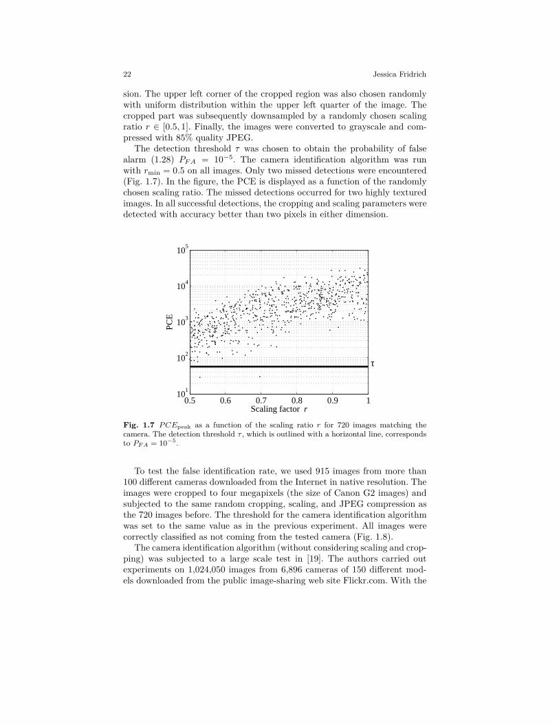
The detection threshold τ was chosen to obtain the probability of falsealarm (1.28) PF A = 10−5. The camera identification algorithm was runwith rmin = 0.5 on all images. Only two missed detections were encountered(Fig. 1.7). In the figure, the PCE is displayed as a function of the randomlychosen scaling ratio. The missed detections occurred for two highly texturedimages. In all successful detections, the cropping and scaling parameters weredetected with accuracy better than two pixels in either dimension.

0.5 0.6 0.7 0.8 0.9 110

1

102

103

104

105

Scaling factor r

PCE

τ

Fig. 1.7 PCEpeak as a function of the scaling ratio r for 720 images matching thecamera. The detection threshold τ , which is outlined with a horizontal line, correspondsto PF A = 10−5.

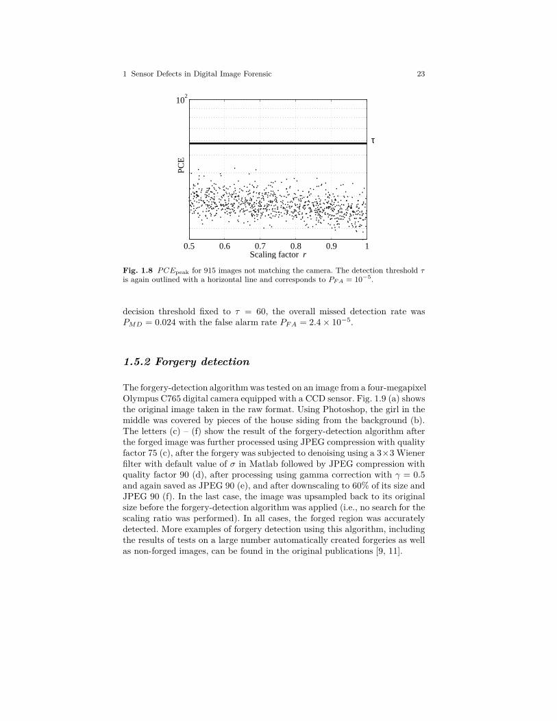
To test the false identification rate, we used 915 images from more than100 different cameras downloaded from the Internet in native resolution. Theimages were cropped to four megapixels (the size of Canon G2 images) andsubjected to the same random cropping, scaling, and JPEG compression asthe 720 images before. The threshold for the camera identification algorithmwas set to the same value as in the previous experiment. All images werecorrectly classified as not coming from the tested camera (Fig. 1.8).

The camera identification algorithm (without considering scaling and crop-ping) was subjected to a large scale test in [19]. The authors carried outexperiments on 1,024,050 images from 6,896 cameras of 150 different mod-els downloaded from the public image-sharing web site Flickr.com. With the


0.5 0.6 0.7 0.8 0.9 1

102

Scaling factor r

PCE

τ

Fig. 1.8 PCEpeak for 915 images not matching the camera. The detection threshold τis again outlined with a horizontal line and corresponds to PF A = 10−5.

decision threshold fixed to τ = 60, the overall missed detection rate wasPMD = 0.024 with the false alarm rate PF A = 2.4× 10−5.

1.5.2 Forgery detection

The forgery-detection algorithm was tested on an image from a four-megapixelOlympus C765 digital camera equipped with a CCD sensor. Fig. 1.9 (a) showsthe original image taken in the raw format. Using Photoshop, the girl in themiddle was covered by pieces of the house siding from the background (b).The letters (c) – (f) show the result of the forgery-detection algorithm afterthe forged image was further processed using JPEG compression with qualityfactor 75 (c), after the forgery was subjected to denoising using a 3×3 Wienerfilter with default value of σ in Matlab followed by JPEG compression withquality factor 90 (d), after processing using gamma correction with γ = 0.5and again saved as JPEG 90 (e), and after downscaling to 60% of its size andJPEG 90 (f). In the last case, the image was upsampled back to its originalsize before the forgery-detection algorithm was applied (i.e., no search for thescaling ratio was performed). In all cases, the forged region was accuratelydetected. More examples of forgery detection using this algorithm, includingthe results of tests on a large number automatically created forgeries as wellas non-forged images, can be found in the original publications [9, 11].

24 Jessica Fridrich

(a) (b)

(c) (d)

(e) (f)

Fig. 1.9 From upper left corner by rows: a) the original image, b) its tampered version,the result of the forgery-detection algorithm after the forged image was processed usingc) JPEG with quality factor 75, d) 3 × 3 Wiener-filtered plus JPEG 90, e) gammacorrection with γ = 0.5 plus JPEG 90, and f) scaled down by factor of 0.6 and JPEG90.

1.6 Fighting the fingerprint-copy attack

Since the inception of camera identification methods based on sensor finger-prints in 2005 [41], researchers have realized that the sensor fingerprint canbe copied onto an image that came from a different camera in an attempt toframe an innocent victim. In the most typical and quite plausible scenario,Alice, the victim, posts her images on the Internet. Eve, the attacker, es-timates the fingerprint of Alice’s camera and superimposes it onto anotherimage. Indeed, as already shown in the original publication and in [17, 46],correlation detectors cannot distinguish between a genuine fingerprint and afake one.

In this section, we describe a countermeasure [23, 12] against this fingerprint-copy attack that enables Alice to prove that she has been framed (that thefingerprint is fake). We assume that Alice owns a digital camera C. Eve takes


an image J from a different camera C′ with fingerprint K′ 6= K and makes itappear as if it was taken by C. She does so by first estimating the fingerprintof C from some set of Alice’s images and then properly adds it to J.

In particular, let us assume that Eve has access to N images, from C andestimates its fingerprint KE using the estimator (1.7). We note that Evecertainly is free to use a different estimator. However, any estimation proce-dure will be some form of averaging of noise residuals W. Having estimatedthe fingerprint, Eve may preprocess J to suppress the PRNU term JK′ in-troduced by the sensor in C′ and/or to remove any artifacts in J that areincompatible with C. Because suppressing the PRNU term is not an easytask [45], quite likely the best option for Eve is to skip this step altogether.This is because the PRNU component JK′ in J is very weak to be detectedper se and because it is unlikely that Alice will gain access to C′. In fact, Eveshould avoid processing J too much as it may introduce artifacts of its own.

If Eve saves her forgery as a JPEG file, she needs to make sure that thequantization table is compatible with camera C, otherwise Alice will knowthat the image has been manipulated and did not come directly from hercamera. If camera C′ uses different quantization tables than C, Eve willinevitably introduce double-compression artifacts into J, giving Alice againa starting point of her defense.

Unless C and C′ are of the same model, the forged image may containcolor-interpolation artifacts of C′ incompatible with those of C. Alice couldleverage techniques developed for camera brand/model identification [7] andprove that there is a mismatch between the camera model and the colorinterpolation artifacts. A knowledgeable attacker may, in turn, attempt toremove such artifacts of C′ and introduce interpolation artifacts of C, forexample, using the method described in [4].

It should now be apparent that it is far from easy to create a “perfect”forgery. While it is certainly possible for Alice to utilize traces of previouscompression or color interpolation artifacts, no attempt is made in this sectionto exploit these discrepancies to reveal the forged fingerprint. Our goal is todevelop techniques capable of identifying images forged by Eve even in themost difficult scenario for Alice when C′ is of exactly the same model as Cto avoid any incompatibility issues discussed above. Thus, Alice cannot takeadvantage of knowing any a priori information about C′.

The final step for Eve is to plant the estimated fingerprint in J, creatingthus the forged image J′. In her attempt to mimic the acquisition process,and in accordance with (1.4), Eve superimposes the fake fingerprint multi-plicatively, which is what would happen if J was indeed taken by C:

J′ = [J(1 + αKE)], (1.37)

where α > 0 is a scalar fingerprint strength and [x] is the operation of round-ing x to integers forming the dynamic range of J. Finally, Eve saves J′ as

26 Jessica Fridrich

JPEG with the same or similar quantization table as that of the originalimage J.

Formula (1.37) should be understood as three equations for each colorchannel of J. This attack indeed succeeds in fooling the camera identificationalgorithm in the sense that the response of the fingerprint detector on J′

(either the correlation (1.19), the generalized matched filter in [11], or thePCE (1.21)) will be high enough to indicate that J′ was taken by camera C.

A very important issue for Eve is the choice of the strength α. Here,we grant Eve the ability to create a “perfect” forgery in the sense that J′

elicits the same response of the fingerprint detector implemented with thetrue fingerprint K as when J′ was indeed taken by C. A good estimate ofthe detector response can be obtained using a predictor, such as the onedescribed in Section 1.4.4. This way, Eve makes sure that the fingerprint isnot suspiciously weak or strong. While it is certainly true that Eve cannoteasily construct the predictor because she does not have access to the truefingerprint K, she may select the correct strength α by pure luck. To be moreprecise here, we grant Eve the ability to guess the right strength insteadof giving her access to K. We note that similar assumptions postulating aclairvoyant attacker are commonly made in many branches of informationsecurity.

1.6.1 Detecting fake fingerprints

Here, we describe a test using which Alice can decide whether an image camefrom her camera or whether it was forged by Eve as described above. Forsimplicity, we only discuss the case when Eve created one forged image J′

and Alice has access to some of the N images used by Eve to estimate KE

but Alice does not know which they are. She has a set of Nc ≥ N candidateimages that Eve may have possibly used. This is a very plausible scenariobecause, unless Eve gains access to Alice’s camera and takes images of herown and then removes them from the camera before returning the camera toAlice, Eve will have little choice but to use images taken by Alice, such asimages posted by Alice on the Internet. In this case, Alice can prove that theforged image did not originally come from her camera by identifying amongher candidate images those used by Eve.

We now explain the key observation based on which Alice can constructher defense. Let I be one of the N images available to Alice that Eve used toforge J′. Since the noise residual of I, WI, participates in the computation ofKE through formula (1.7), J′ will contain a scaled version of the entire noiseresidual WI = IK + ΞI. Thus, besides the PRNU term, WI and WJ′ willshare another signal – the noise ΞI. Consequently, the correlation cI,J′ =corr(WI, WJ′) will be larger than what it would be if the only commonsignal between I and J′ was the PRNU component (which would be the case


if J′ was not forged). As this increase may be quite small and the correlationitself may fluctuate significantly across images, the test that evaluates thestatistical increase must be calibrated. We call this test the triangle test.

WI WJ′

KA

corr

corrcorr

Fig. 1.10 Diagram for the triangle test.

Alice starts her defense by computing an estimate of the fingerprint ofher camera KA from images guaranteed to not have been used by Eve. Forinstance, she can take new images with her camera C. Then, for a can-didate image I, she computes cI,J′ , c

I,KA= corr(WI, KA), and c

J′,KA=

corr(WJ′ , KA) (follow Fig. 1.10). The test is based on the fact that for im-ages I that were not used to forge J′, the value of cI,J′ can be estimated fromc

I,KAand c

J′,KAwhile when I was used in the forgery, the correlation cI,J′

will be higher than its estimate.In order to obtain a more accurate relationship, similar to our approach to

forgery detection in Section 1.4.4, we will work by blocks of pixels, denotingthe signals constrained to block b with subscript b. We adopt the model (1.4)for the noise residuals and a similar model for Alice’s fingerprint:

WI,b = aI,bIbKb + ΞI,b, (1.38)

WJ′,b = aJ′,bJ′bKb + ΞJ′,b, (1.39)

KA = Kb + ξb. (1.40)

The block-dependent attenuation factor a in (1.39) has been introduceddue to the fact that various image processing that might have been appliedby Eve to J may affect the PRNU factor differently in each block.

When I was not used by Eve, under some fairly mild assumptions aboutthe noise terms in (1.39), the following estimate of cI,J′ is derived in [12, 23]

cI,J′ = corr(WI, KA)corr(WJ′ , KA)µ(I, J′)q−2, (1.41)

where µ(I, J′) is the “mutual-content factor,”

µ(I, J′) =

∑

b aI,baJ′,bIbJ′b

∑

b aI,bIb ·∑

b aJ′,bJ′b

NB, (1.42)

28 Jessica Fridrich

and the bar denotes the sample mean as before. The integer NB is the numberof blocks and q ≤ 1 is the quality of KA, q−2 = 1 + (SNR

KA)−1, SNR

KA=

‖K‖2 / ‖ξ‖2.The attenuation factors can be estimated by computing the following

block-wise correlations:1

aI,b =‖WI,b‖

√

I2b

∥

∥

∥KA,b

∥

∥

∥

corr(WI,b, KA,b)q−2. (1.43)

Continuing the analysis of the case when I was not used by Eve, we con-sider cI,J′ and cI,J′ as random variables over different images I for a fixedJ′. The dependence between these two random variables is well fit with astraight line cI,J′ = λcI,J′ + c0. Because the distribution of the deviationfrom the linear fit does not seem to vary with cI,J′ (see Fig. 1.11), we makea simplifying assumption that the conditional probability

Pr(cI,J′ − λcI,J′ − c0 = x|cI,J′) ≈ fJ′(x), (1.44)

is independent of cI,J′.When I was used by Eve in the multiplicative forgery, due to the additional

common signal ΞI, the correlation cI,J′ increases to βcI,J′ , where β is thefollowing multiplicative factor derived in [23, 12]

β = 1 +α

N

∑

b aJ′,bJ′b ‖ΞI,b‖2

∑

b aI,baJ′,bIbJ′b ‖Kb‖2 . (1.45)

Notice that the percentual increase is proportional to the fingerprintstrength α and the energy of the common noise component ΞI,b; it is in-versely proportional to N .

Alice now runs the following composite binary hypothesis test for everycandidate image I from her set of Nc candidate images:

H0 : cI,J′ − λcI,J′ − c0 ∼ fJ′(x),

H1 : cI,J′ − λcI,J′ − c0 � fJ′(x). (1.46)

The reason why (1.46) cannot be turned into a simple hypothesis test isthat the distribution of cI,J′ when I is used for forgery is not available to Aliceand it cannot be determined experimentally because Alice does not know theexact actions of Eve. Thus, we resort to the Neyman-Pearson test and setour decision threshold τ to bound the probability of false alarm,

Pr(cI,J′ − λcI,J′ − c0 > τ |H0) = PF A. (1.47)

1 Equation (1.43) holds independently of whether or not I was used by Eve.


The pdf fJ′(x) is often very close to a Gaussian but for some images J′,the tails exhibit a hint of a polynomial dependence. Thus, to be conservative,we used Student’s t-distribution for the fit.

Note that, depending on J′, the constant of proportionality λ > 1,which suggests the presence of an unknown multiplicative hidden parameterin (1.41) most likely due to some non-periodic NUAs that were not removedusing zero-meaning as described in Section 1.3.1. The quality of Alice’s fin-gerprint, q, can be considered unknown (or simply set to 1) as different q willjust correspond to a different λ (scaling of the x axis in the diagram of cI,J′

versus cI,J′).Alice now has two options. She can test each candidate image I separately

by evaluating its p-value and thus, on a certain level of statistical significance,identify those images that were used by Eve for estimating her fingerprint.Alternatively, Alice can test for Nc candidate images I all at once whethercI,J′ − λcI,J′ − c0 ∼ fJ′(x). This “pooled test” will be a better choice forher for large N when the reliability of the triangle test for individual imagesbecomes low.

1.6.2 Experiments

In this chapter, we report the results of experiments when testing individualimages. The original publications [23, 12] contain much more detailed exper-imental evaluation including the pooled test and another case when multipleforged images are analyzed.

In the experiment, the signals entering the triangle test were preprocessedby zero-meaning. Wiener filtering, as described in Section (1.3.1) to suppressthe NUAs, was only applied to WJ′ and not to WI to save computationtime. The camera C′ is the four-megapixel Canon PS A520 while C is CanonPS G2, which has the same native resolution. Both cameras were set to takeimages at the highest quality JPEG compression and the largest resolution.The picture-taking mode was set to “auto.”

The fingerprint estimation algorithm and the forging algorithm depend ona large number of parameters, such as the parameters of the denoising filter.In presenting our test results, we intentionally opted for what we considerto be the most advantageous setting for Eve and the hardest one for Alice.This way, the results will be on the conservative side. Furthermore, to obtaina compact yet comprehensive report on the performance of the triangle test,the experiments were designed to show the effect of only the most influentialparameters. To estimate her fingerprint KE , Eve uses the most accurateestimator she can find in the literature (1.7) implemented using the denoisingfilter F described in [43] with the wavelet-domain Wiener filter parameterσ = 3 (valid for 8-bit per channel color images). From our experiments,

30 Jessica Fridrich

the reliability of the triangle test is insensitive to the denoising filter or themismatch between the filters used by Eve and Alice.

Then, Eve forges a 24-bit color image J from camera C′ to make it lookas if it came from camera C. She first slightly denoises J using the samedenoising filter F (with its Wiener filter parameter σ = 1) to suppress thefingerprint from camera C′ and possibly other artifacts introduced by C′.The filter is applied to each color channel separately. Then, Eve adds thefingerprint to J, using (1.37), and saves the result as JPEG with qualityfactor 90, which is slightly smaller than the typical qualities of the originalJPEG images J. The fingerprint strength factor α is determined so that theresponse of the generalized matched filter (Equation (11) in [11]) matchesits prediction obtained using the predictor as described in Section (1.4.4).The predictor was implemented as a linear combination of intensity (1.31),texture (1.33), and flattening features (1.32), and their second-order terms.The coefficients of the linear fit were determined from 20 images of naturalscenes using the least square fit. Note that because Eve needs to adjust α sothat the JPEG-compressed J′ elicits the same GMF value as the prediction,the proper value of α must be found, e.g., using a binary search. Finally, thetrue fingerprint K was estimated from 300 JPEG images of natural scenes.

On the defense side, Alice estimates her fingerprint KA from NA = 15blue-sky raw images (fingerprint quality was q = 0.56). Surprisingly, thequality of KA has little impact on the triangle test. Tests with NA = 70produced essentially identical results. In particular, it is not necessary forAlice to work with a better quality fingerprint than Eve! In all experiments,the block size was 128× 128 pixels. The triangle test performed equally wellfor blocks as small as 64× 64 and as large as 256× 256.

We now evaluate the performance of the triangle test when applied toeach candidate image individually. By far the most influential element is thenumber of images used by Eve, N , and the content of the forged image J.Six randomly selected test images J shown in Fig. 1.12 were tested with thevalues of N ∈ {20, 50, 100, 200}. To give the reader a sense of the extent ofEve’s forging activity, in Table 1.1 we report the PSNR between J and J′

before it is JPEG compressed. The PSNR between J′ and F (J′) measuresthe total distortion that includes the slight denoising, F (J), and quantizationto 24-bit colors after adding the fingerprint. The PSNR between J′ and theslightly denoised F (J) measures the energy of the PRNU term only.

To accurately estimate the probability distribution fJ(x), we used 358images from camera C that were for sure not used by Eve. All these imageswere taken within a period of about four years. In practice, depending on thesituation, statistically significant conclusions may be obtained using a muchsmaller sample.

Fig. 1.11 presents a typical plot of cI,J′ versus cI,J′ for N = 20 andN = 100. As expected, the separation between images used by Eve andthose not used deteriorates with increasing N . When applying the triangletest individually to each candidate image, after setting the decision threshold


0 0.005 0.01 0.015 0.02 0.0250

0.005

0.01

0.015

0.02

0.025

0.03

0.035

0.04

0.045


Tru

e co

rrel

atio

n

Images not used by EveImages used by Eve

0 0.005 0.01 0.015 0.02 0.025 0.030

0.005

0.01

0.015

0.02

0.025

0.03

0.035

0.04

0.045


Tru

e co

rrel

atio

n

Images not used by EveImages used by Eve

Fig. 1.11 True correlation cI,J′ versus the estimate cI,J′ for image no. 5. Eve’s finger-print was estimated from N = 20 images (top) and N = 100 (bottom).

32 Jessica Fridrich

to satisfy a desired probability of false alarm, PF A, the probability of cor-rect detection PD in the hypothesis test (1.46) is shown in Table 1.2. Eachvalue of PD was obtained by running the entire experiment as explained inSection 1.6.1 and evaluating the p-values for all images used by Eve.

# PSNR(F (J), J′) [dB] PSNR(J, J′) [dB]N 20 50 100 200 20 50 100 200

1 48.8 51.8 53.2 53.9 47.6 49.5 50.3 50.72 49.0 51.8 53.1 53.8 47.8 49.8 50.6 50.93 50.1 51.8 52.9 53.4 48.7 49.8 50.5 50.84 54.5 56.4 57.5 58.7 49.5 50.0 50.2 50.45 49.5 52.2 53.2 54.0 47.7 49.3 49.7 50.16 50.8 53.2 54.3 55.1 49.3 51.0 51.6 52.1

Table 1.1 PSNR between the original image J and the forgery J′ before JPEG com-pression for six test images.

# PD [%] for PF A = 10−3 PD [%] for PF A = 10−4

N 20 50 100 200 20 50 100 200

1 100 92 63 15 100 80 44 62 100 84 40 5 100 74 26 03 95 78 35 4 95 66 14 04 95 64 21 3 95 42 8 15 100 90 56 11 100 82 41 26 100 94 59 14 100 90 40 2

Table 1.2 Detection rate in percents for six text images.

The lower detection rate for image no. 4 is due to the low energy of thefingerprint (see the corresponding row in Table 1.1) dictated by the predictor.Because the image has smooth content, which is further smoothened by thedenoising filter, the fingerprint PSNR in the noise residual W is higher thanfor other images. Consequently, a low fingerprint energy is sufficient in match-ing the predicted correlation. Image no. 3 also produced lower detection rates,mostly due to the fact that 26% of the image content is overexposed (the en-tire sky) with fully saturated pixels. The attenuation factor ab in (1.39) isthus effectively equal to zero for such blocks b, while it is estimated in (1.43)under H1 as being relatively large due to the absence of the noise term ΞJ′,b.A possible remedy is to apply the triangle test only to the non-saturatedpart of the image. However, then we experience a lower accuracy again dueto a smaller number of pixels in the image. At this point, we note that ifthe attacker makes the forgery using (1.37) without attenuating the PRNUin saturated areas, the fingerprint will be too strong there, which could beused by Alice to argue that the fingerprint has been artificially added andthe image did not come from her camera.


Fig. 1.12 Six original images J from a Canon PS A520 numbered by rows (#1, #2,#3); (#4, #5, #6).

We conclude this section with the statement that while it is possible tomaliciously add a sensor fingerprint to an image to frame an innocent victim,adding it so that no traces of the forging process are detectable appearsrather difficult. The adversary, Eve, will likely have to rely on images takenby Alice that she decided to share with others, for example on her Facebooksite. However, the estimation error of the camera fingerprint estimated fromsuch images will contain remnants of the entire noise residual from all imagesused by Eve. This fact is the basis of the triangle test using which Alice canidentify the images that Eve used for her forgery and, in doing so, prove herinnocence.

As a final remark, we note that while the reliability of the single-imagetriangle test breaks up at approximately N = 100, the test in its pooled form(which is described in [23, 12]) can be applied even when Eve uses a high-quality fingerprint estimated from more than 300 images. The reliability ingeneral decreases with increasing ratio Nc/N .

The reliability of the triangle test can be somewhat decreased by modifyingthe fingerprint estimation process to limit outliers in the noise residuals of im-ages used for the estimation [5, 39]. This will generally suppress the remnantsof the noise residual used by the triangle test. More extensive tests, however,appear necessary to investigate the overall impact of this counter–counter-counter measure on the reliability of the identification algorithm when thefingerprint is not faked.

34 Jessica Fridrich

1.7 Temporal forensics

The goal of temporal forensics is to establish causal relationship among twoor more objects [42, 44]. In this section, we show how pixel defects can beused to order images by their acquisition time given a set of images from thesame camera whose time ordering is known.2 Even though temporal data istypically found in the EXIF header, it may be lost when processing or editingimages off-line. Additionally, since the header is easily modifiable, it cannotbe trusted. Developing reliable methods for establishing temporal order be-tween individual pieces of evidence is of interest for multiple reasons. Suchtechniques can help reveal deception attempts of an adversary or a criminal.The causal relationship also provides information about the whereabouts ofthe photographer.

Strong point defects (hot/stuck pixels) occur randomly in time and spaceon the sensor independently of each other [38, 36, 37, 13], which makes themuseful for determining an approximate age of digital photographs. New defectsappear suddenly and with a constant rate (It is a Poisson process.), whichmeans that the time between the onsets of new defects follows the exponentialdistribution. Once a defect occurs, it becomes a permanent part of the sensorand does not heal itself.

The main cause of new pixel defects is environmental stress, primarily dueto impacting cosmic rays. In general, smaller pixels are more vulnerable topoint defects than larger pixels. Sensors age both at high altitudes and at thesea level. They do age faster at high altitudes or during airplane trips wherecosmic radiation is stronger. Consequently, in real life the defect accumulationmay not be linear in time.

The main technical problem for using point defects for temporal forensics isthat such defects may not be easily detectable in individual images, dependingon the image content, camera settings, exposure time, etc. In the next section,we describe a method for estimating pixel defect parameters and use it fordetermining an approximate age of a digital photograph using the principleof maximum likelihood.

1.7.1 Estimating point defects

Even though sensor defects can be easily estimated in a laboratory environ-ment by taking test images under controlled conditions, a forensic analystmust work with a given set of images taken with camera settings that maybe quite unfavorable for estimating certain defects. For example, the darkcurrent is difficult to estimate reliably from images of bright scenes takenwith a short exposure time and low ISO.

2 Temporal ordering of digital images was for the first time considered in [42].


Let Yk, k = 1, . . . , d, be d images of regular scenes taken at known timest1, . . . , td. As in the previous section, we work with noise residuals Wk = Yk−F (Yk) obtained using a denoising filter F . Since hot pixels (and stuck pixelswith a large offset) are spiky in nature, denoising filters of the type [43] thatextract additive white Gaussian noise are likely a poor choice for estimatingpoint defects. Instead, non-linear filters, such as the median filter, are morelikely to extract the spike correctly.

We use the model of pixel output (1.3):

Wk(i) = Ik(i)K(i) + τkD(i) + c(i) + Ξk(i), (1.48)

where k and i are the image and pixel indices, respectively. For simplicity,we model Ξk(i), k = 1, . . . , d, as an i.i.d. Gaussian sequence with zero meanand variance σ2(i). The known quantities in the model are Ik ≈ F (Yk) andτk; Wk are observables.

From now on, all derivations will be carried out for a fixed pixel i. Thiswill allow us to drop the pixel index and make the expressions more compact.The unknown vector parameter θ = (K, D, c, σ) (for a fixed pixel, θ ∈ R

4)can be estimated using the Maximum Likelihood (ML) principle:

θ = arg maxθ

L(W1, . . . , Wd|θ), (1.49)

where L is the likelihood function

L(W1, . . . , Wd|θ) = (2πσ2)−d/2 exp

(

− 1

2σ2

d∑

k=1

(Wk − IkK− τkD− c)2

)

.

(1.50)Because the modeling noise Ξk is Gaussian, the ML estimator becomes theleast squares estimator [31]. Additionally, the model linearity allows us tofind the maximum in (1.54) in the following well-known form:

(K, D, c) = (HH′)−1H′W, (1.51)

σ2 =1

d

d∑

k=1

(

Wk − IkK− τkD− c)2

, (1.52)

where

H =

I1(i) τ1 1I2(i) τ2 1· · · · · · · · ·

Id(i) τd 1

(1.53)

is a matrix of known quantities and W = (W1, . . . , Wd)′ the vector of ob-servations (noise residuals).

36 Jessica Fridrich

1.7.2 Determining defect onset

We now extend the estimator derived above to the case when we have observa-tions (pixel intensities) across some time span during which the pixel becomes

defective. Our goal is to estimate θ before and after the onset, θ(0), θ(1), andthe onset time j. The estimator derived in the previous section easily extendsto this case

(θ(0)

, θ(1)

, j) = arg max(θ(0),θ(1),j)

Lj(W1, . . . , Wd|θ(0), θ(1)), (1.54)

where

Lj(W1, . . . , Wd|θ(0), θ(1)) = L(W1, . . . , Wj|θ(0))× L(Wj+1, . . . , Wd|θ(1))(1.55)

is the likelihood function written in terms of (1.50). Because of the formof (1.55), the maximization in (1.54) factorizes:

(θ(0)

, θ(1)

, j) = arg maxj

{

arg maxθ(0)

L(W1, . . . , Wj |θ(0))×

arg maxθ(1)

L(Wj+1, . . . , Wd|θ(1))

}

, (1.56)

which converts the problem of onset estimation to the problem of estimatingpixel defect addressed in the previous section.

1.7.3 Determining approximate acquisition time

We are now ready to develop the algorithm for placing a given image I underinvestigation among other d images, I1, . . . , Id, whose time of acquisition isknown, monotone increasing, and whose pixel defects are known, includingthe onset time and the parameters before and after the onset. This problemis again addressed using the ML approach. This time, only the time indexj of I is the unknown as the parameters of all defective pixels are alreadyknown. Denoting the set of all defective pixels D, the estimator becomes:

j = arg maxj

∏

i∈D

L(WI(i)|θ[j>j(i)](i)) (1.57)

written in terms of (1.50). The superscript of θ is the Iverson bracket.


1.7.4 Performance example

We applied the approach outlined above to images from a Canon PS sd400digital camera. Total of d = 329 images with known acquisition times span-ning almost 900 days were used to estimate the defect parameters for 46 pointdefects. Then, the acquisition times were estimated for 159 other images. Theaccuracy with which one can estimate the time obviously depends on howmany new defects appear during the entire time span.

The noise residual W was extracted using a 3× 3 median filter. Fig. 1.13shows the true date versus the estimated date for all 159 images. The circleson the diagonal correspond to the training set of 329 images with knowndates. They show the temporal distribution of training images. Note that notraining images appear between time 400 and 500, limiting thus our abilityto date images within this time interval.

0 200 400 600 8000

100

200

300

400

500

600

700

800

900

True time

Est

imat

ed ti

me

Test imagesTraining images

Fig. 1.13 True acquisition date versus date estimated using (1.57) based on detectingpixel defects. The average absolute error between the estimated and true date was 61.56days.

1.7.5 Confidence intervals

In forensic setting, the analyst will likely be interested in statements of thetype “the probability that image I was taken in time interval [t, t′] is at leastp.” The approach outlined above allows us to quantify the results in this waybecause the conditional probabilities Pr(WI|j) =

∏

i∈D L(WI(i)|θ[j>j(i)](i))are known for each j. From the Bayes formula,

38 Jessica Fridrich

Pr(j|WI) = Pr(WI|j)Pr(j)

Pr(WI). (1.58)

Thus, the probability that I was taken in time interval [t, t′] is

Pr(j ∈ [t, t′]|WI) =

∑

k∈[t,t′] Pr(WI|k)Pr(k)∑

k Pr(WI|k)Pr(k). (1.59)

Depending on the situation at hand, the prior probabilities Pr(k) may beknown from other forensic evidence or may be completely unknown. In theabsence of any information about the priors, one could resort to the principleof maximum uncertainty and assume the least informative prior distribution– that the owner of the camera was taking images at a uniform rate, leadingto Pr(k) = 1/(tk− tk−1) for all k, where tk is the time when the kth trainingimage was taken.

1.8 Summary

Every imaging sensor contains defects and imperfections that can be utilizedfor a variety of forensic tasks. The photo-response non-uniformity (PRNU)plays the role of a fingerprint that well survives processing and can thus beused for identifying images taken by a camera whose fingerprint is known. Itsabsence in individual regions testifies about malicious processing applied toan image (forgery detection). The fingerprint can also serve as a template torecover previously applied geometrical processing. The methodology appliesto CCD as well as CMOS sensors and to digital still and video cameras aswell as scanners [25, 16, 34].

Although it is possible for an adversary to superimpose a camera finger-print onto an image from a different camera and thus frame an innocentvictim (the fingerpint-copy attack), it is not easy to do this without leavingdetectable traces. The so-called triangle test can reveal when a fingerprinthas been maliciously added and one can even identify the images that theadversary utilized in the attack.

Besides PRNU, sensors also contain the so-called point defects, examplesof which are hot and stuck pixels and pixels with abnormal sensitivity. Suchdefects occur randomly on the sensor and randomly in time. This makesthem useful for determining an approximate time when an image was taken.This chapter outlines a maximum-likelihood estimator of time of acquisitionthat basically detects the presence of point defects with a known onset in animage.

The performance of all forensic methods introduced here is briefly demon-strated on real images. Throughout the text, references to previously pub-


lished articles guide the interested reader to more detailed technical informa-tion.

1.8.1 Related publications

When the camera identification technique is deployed on a large scale, onequickly runs into complexity issues. For example, the seemingly routine taskof matching an image (or fingerprint) to a large database of fingerprints storedin a database may be quite time consuming already when the database holdsmerely hundreds of fingerprints. This is because correlating each databasefingerprint with the query signal may take hours even in the simplest casewhen no search for geometrical transformation is carried out. To address thisproblem, researchers [24] introduced the concept of a fingerprint digest andsparse data structures to cut down the searching time significantly.

A similar task of matching a large database of images to a small numberof fingerprints was proposed in [2]. Here, the complexity was decreased usinga hierarchical binary search.

For completeness, we note that there exist approaches combining sensornoise defects with machine-learning classification [25, 33, 6]. An older versionof this forensic method was tested for cell phone cameras in [6] and in [47]where the authors show that a combination of sensor-based forensic methodswith methods that identify camera brand can decrease false alarms. The im-provement reported in [47], however, is unlikely to hold for the newer versionof the sensor noise forensic method presented in this chapter as the resultsof [47] appear to be influenced by uncorrected non-unique artifacts discussedin Section 1.3.1. The problem of pairing of a large number of images was stud-ied in [3] using an ad hoc approach. A large-scale experimental evaluationof camera identification on over one million images from over 6,800 camerascovering 150 models appears in [19]. Identification of printed images is thesubject of [20]. Anisotropy of image noise for classification of images intoscans, digital camera images, and computer art appeared in [33]. The effectof denoising filters on the performance of sensor-based camera identificationwas studied in [1].

1.8.2 Real-life applications

Camera identification based on sensor fingerprints described in this chapterpassed the Daubert challenge http://en.wikipedia.org/wiki/Daubert_

standard in the State of Alabama in July 2011. In March 2009, MiroslavGoljan testified in Scotland as an expert witness in a high-profile case that in-volved child abuse crimes by a pedophile ring. See the article “Operation Alge-

40 Jessica Fridrich

bra” at http://p10.hostingprod.com/@spyblog.org.uk/blog/2009/05/.Cases involving movie piracy and illegal acquisition and distribution of moviestaped inside a movie theater form another area of possible applications ofthis technology. The sensor fingerprint can also be used to reverse-engineerin-camera geometrical processing, such as digital zoom or correction of lensdistortion, and to provide a blind estimate of the focal length at which animage was taken [22].

ACKNOWLEDGMENT

The work on this chapter was partially supported by the NSF grant numberCNF-0830528. The U.S. Government is authorized to reproduce and dis-tribute reprints for Governmental purposes notwithstanding any copyrightnotation there on. The views and conclusions contained herein are those ofthe authors and should not be interpreted as necessarily representing theofficial policies, either expressed or implied, of Air Force Office of ScientificResearch or the U.S. Government. The author would like to thank MiroslavGoljan for useful discussions.

References

1. I. Amerini, R. Caldelli, V. Cappellini, F. Picchioni, and A. Piva. Analysis of de-noising filters for photo-response non-uniformity noise extraction in source cameraidentification. In Proc. of the 16th international conference on Digital Signal Pro-cessing, pages 511–517, 2009.

2. S. Bayram, H. T. Sencar, and N. Memon. Efficient techniques for sensor fingerprintmatching in large image and video databases. In N. Memon and J. Dittmann,editors, Proceeedings of SPIE Electronic media Forensics and Security XII, volume7541, pages 09–01–09–12, January 2010.

3. G. J. Bloy. Blind camera fingerprinting and image clustering. IEEE Transactionson Pattern Analysis and Machine Intelligence, 30(3):532–534, March 2008.

4. R. Böhme and M. Kirchner. Synthesis of color filter array pattern in digital images.In N. Memon and J. Dittmann, editors, Proc. SPIE, Media Forensics and SecurityXI, volume 7254, pages 0K–0L, San Jose, CA, January 18–22 2009.

5. R. Caldelli, I. Amerini, and A. Novi. An analysis on attacker actions in fingerprint-copy attack in source camera identification. In Proc. IEEE WIFS, Iguazu Falls,Brazil, November 29 – December 2 2011.

6. O. Çeliktutan, I. Avcibas, and B. Sankur. Blind identification of cellular phone cam-eras. In E.J. Delp and P.W. Wong, editors, Proc. SPIE Electronic Imaging, Steganog-raphy, Security, and Watermarking of Multimedia Contents IX, volume 6505, pagesH1–H12, January 2007.

7. O. B. Celiktutan, B. Sankur, and I. Avcibas. Blind identification of source cell-phonemodel. IEEE Transactions on Information Forensics and Security, 3(3):553–566,2008.

8. M. Chen, J. Fridrich, and M. Goljan. Digital imaging sensor identification (fur-ther study). In E.J. Delp and P.W. Wong, editors, Proc. SPIE Electronic Imag-


ing, Steganography, Security, and Watermarking of Multimedia Contents IX, volume6505, pages 0P–0Q, January 2007.

9. M. Chen, J. Fridrich, and M. Goljan. Imaging sensor noise as digital x-ray for re-vealing forgeries. In T. Furon et al., editor, Proc. 9th Information Hiding Workshop,Saint Malo, France, volume 4567 of LNCS, pages 342–358. Springer-Verlag, June2007.

10. M. Chen, J. Fridrich, and M. Goljan. Source digital camcorder identification usingccd photo response nonuniformity. In E.J. Delp and P.W. Wong, editors, Proc.SPIE Electronic Imaging, Steganography, Security, and Watermarking of MultimediaContents IX, volume 6505, pages 1G–1H, January 2007.

11. M. Chen, J. Fridrich, and M. Goljan. Determining image origin and integrity usingsensor noise. IEEE Transactions on Information Forensics and Security, 1(1):74–90,March 2008.

12. M. Chen, J. Fridrich, and M. Goljan. Defending against fingerprint-copy attack insensor-based camera identification. IEEE Transactions on Information Security andForensics, 2010. submitted.

13. J. Dudas, L. M. Wu, C. Jung, G. H. Chapman, Z. Koren, and I. Koren. In R. A.Martin, J. M. DiCarlo, and N. Sampat, editors, Identification of in-field defect de-velopment in digital image sensors, volume 6502, page 65020Y. SPIE, 2007.

14. T. Filler, J. Fridrich, and M. Goljan. Using sensor pattern noise for camera modelidentification. In Proc. IEEE International Conference on Image Processing (ICIP),October 2008.

15. A. El Gamal, B. Fowler, H. Min, and X. Liu. Modeling and estimation of FPNcomponents in CMOS image sensors. In Proc. SPIE Solid State Sensor Arrays:Development and Applications II, volume 3301-20, pages 168–177, January 1998.

16. T. Gloe, E. Franz, and A. Winkler. Forensics for flatbed scanners. In E.J. Delpand P.W. Wong, editors, Proc. SPIE Electronic Imaging, Steganography, Security,and Watermarking of Multimedia Contents IX, volume 6505, pages 1I–1J, January2007.

17. T. Gloe, M. Kirchner, A. Winkler, and R. Boehme. Can we trust digital imageforensics? In Proc. The 15th International conference on Multimedia, Multimedia’07, ACM, pages 78–86, 2007.

18. M. Goljan, M. Chen, and J. Fridrich. Identifying common source digital camerafrom image pairs. In Proc. IEEE International Conference on Image Processing(ICIP), September 2007.

19. M. Goljan, T. Filler, and J. Fridrich. Camera identification – large scale test. InN. Memon and J. Dittmann, editors, Proceeedings of SPIE Electronic media Foren-sics and Security XI, volume 7254, pages 0I–01–0I–12, January 2009.

20. M. Goljan and J. Fridrich. Camera identification from printed images. In E.J. Delp,P. W. Wong, N. Memon, and J. Dittmann, editors, Proceeedings of SPIE ElectronicImaging, Security, Forensics, Steganography, and Watermarking of Multimedia Con-tents X, volume 6819, pages OI1–OI12, January 2008.

21. M. Goljan and J. Fridrich. Camera identification from scaled and cropped images.In E. Delp, P. W. Wong, N. Memon, and J. Dittmann, editors, Proceeedings ofSPIE Electronic Imaging, Security, Forensics, Steganography, and Watermarking ofMultimedia Contents X, volume 6819, pages OE1–OE13, January 2008.

22. M. Goljan and J. Fridrich. Sensor-fingerprint based identification of images correctedfor lens distortion. In N. D. Memon, A. Alattar, and E. J. Delp, editors, Proceed-ings SPIE, Electronic Imaging, Media Watermarking, Security and Forensics 2012,January 22–26, 2012.

23. M. Goljan, J. Fridrich, and M. Chen. Sensor noise camera identification: Counter-ing counter-forensics. In N. Memon, J. Dittmann, and A. Alattar, editors, Proc.SPIE Electronic Imaging, Steganography, Security, and Watermarking of Multime-dia Contents XII, volume 7541, pages 0S–01–0S–12, January 17–21 2010.

42 Jessica Fridrich

24. M. Goljan, J. Fridrich, and T. Filler. Managing a large database of camera finger-prints. In N. Memon, J. Dittmann, and A. Alattar, editors, Proceeedings of SPIEElectronic media Forensics and Security XII, volume 7541, pages 08–01–08–12, Jan-uary 2010.

25. H. Gou, A. Swaminathan, and M. Wu. Robust scanner identification based onnoise features. In E.J. Delp and P.W. Wong, editors, Proc. SPIE Electronic Imag-ing, Steganography, Security, and Watermarking of Multimedia Contents IX, volume6505, pages 0S–0T, January 2007.

26. G. Healey and R. Kondepudy. Radiometric CCD camera calibration and noiseestimation.

27. G. E. Healey and R. Kondepudy. Radiometric CCD camera calibration and noiseestimation. IEEE Transactions on Pattern Analysis and Machine Intelligence,16(3):267–276, March 1994.

28. G. C. Holst. CCD Arrays, Cameras, and Displays. JCD Publishing & SPIE Press,USA, 2nd edition, 1998.

29. C. R. Holt. Two-channel detectors for arbitrary linear channel distortion. IEEETransactions on Acoustics, Speech, and Signal Processing, ASSP-35(3):267–273,March 1987.

30. J.R. Janesick. Scientific Charge-Coupled Devices, volume PM83. SPIE Press Mono-graph, 2001.

31. S. M. Kay. Fundamentals of Statistical Signal Processing, Volume I: EstimationTheory, volume II. Upper Saddle River, NJ: Prentice Hall, 1998.

32. S.M. Kay. Fundamentals of Statistical Signal Processing, Detection Theory, vol-ume II. Prentice Hall, 1998.

33. N. Khanna, A. K. Mikkilineni, G. T. C. Chiu, J. P. Allebach, and E. J. Delp. Forensicclassification of imaging sensor types. In E.J. Delp and P.W. Wong, editors, Proc.SPIE Electronic Imaging, Steganography, Security, and Watermarking of MultimediaContents IX, volume 6505, pages U1–U9, January 2007.

34. N. Khanna, A.K. Mikkilineni, G.T.C. Chiu, J.P. Allebach, and E.J. Delp. Scanneridentification using sensor pattern noise. In E.J. Delp and P.W. Wong, editors, Proc.SPIE, Electronic Imaging, Security, Steganography, and Watermarking of Multime-dia Contents IX, volume 6505, January.

35. K. Kurosawa, K. Kuroki, and N. Saitoh. CCD fingerprint method – identificationof a video camera from videotaped images. In Proc. IEEE International Conferenceon Image Processing (ICIP), pages 537–540, October 1999.

36. J. Leung, G. H. Chapman, I. Koren, and Z. Koren. Automatic detection of in-field defect growth in image sensors. In DFT ’08: Proceedings of the 2008 IEEEInternational Symposium on Defect and Fault Tolerance of VLSI Systems, pages305–313, Washington, DC, 2008. IEEE Computer Society.

37. J. Leung, G. H. Chapman, I. Koren, and Z. Koren. Characterization of gain enhancedin-field defects in digital imagers. Defect and Fault-Tolerance in VLSI Systems,IEEE International Symposium on, 0:155–163, 2009.

38. J. Leung, J. Dudas, G. H. Chapman, I. Koren, and Z. Koren. Quantitative analysisof in-field defects in image sensor arrays. In Defect and Fault-Tolerance in VLSISystems, 2007. DFT ’07. 22nd IEEE International Symposium on, pages 526–534,September 2007.

39. C.-T. Li. Source camera identification using enhanced sensor pattern noise. In Proc.of IEEE ICIP, pages 7–11, 2009.

40. J. Lukáš, J. Fridrich, and M. Goljan. Determining digital image origin using sensorimperfections. In E. J. Delp and P. W. Wong, editors, Proceedings SPIE, ElectronicImaging, Security, Steganography, and Watermarking of Multimedia Contents VII,pages 249–260, San Jose, CA, January 16–20, 2005.

41. J. Lukáš, J. Fridrich, and M. Goljan. Digital camera identification from sensorpattern noise. IEEE Transactions on Information Forensics and Security, 1(2):205–214, June 2006.


42. J. Mao, O. Bulan, G. Sharma, and S. Datta. Device temporal forensics: An in-formation theoretic approach. In Proc. IEEE International Conference on ImageProcessing (ICIP), volume 1, November 2009.

43. M. K. Mihcak, I. Kozintsev, K. Ramchandran, and P. Moulin. Low-complexityimage denoising based on statistical modeling of wavelet coefficients. IEEE SignalProcessing Letters, 6(12):300–303, December 1999.

44. A. D. Rosa, F. Uccheddu, A. Costanzo, A. Piva, and M. Barni. Exploring imagedependencies: a new challange in image forensics. In N. Memon, J. Dittmann, andA. Alattar, editors, Proceeedings of SPIE Electronic media Forensics and SecurityXII, volume 7541, pages 0X–1–0X–12, January 2010.

45. K. Rosenfeld and H. T. Sencar. A study of the robustness of PRNU-based cameraidentification. In N. Memon, J. Dittmann, and A. Alattar, editors, Proc. SPIE Elec-tronic Imaging, Steganography, Security, and Watermarking of Multimedia ContentsXI, volume 7254, pages 0M–0N, January 18–22 2009.

46. M. Steinebach, H. Liu, P. Fan, and S. Katzenbeisser. Cell phone camera ballistics:attacks and countermeasures. In Proc. SPIE, Multimedia on Mobile Devices 2010,volume 7542, pages 0B–0C, San Jose, CA, January 18–22 2010.

47. Y. Sutcu, S. Bayram, H.T. Sencar, and N. Memon. Improvements on sensor noisebased source camera identification. In IEEE International Conference on Multimediaand Expo, pages 24–27, July 2007.

Chapter 1 Sensor Defects in Digital Image...

Documents

Transcript of Chapter 1 Sensor Defects in Digital Image...