Ordinary di⁄erential equations and mathematical modelling ...
CHAPTER � TREFETHEN ���� � �
Chapter ��
Ordinary Di�erential Equations
���� Initial value problems
���� Linear multistep formulas
���� Accuracy and consistency
���� Derivation of linear multistep formulas
���� Stability
���� Convergence and the Dahlquist Equivalence Theorem
���� Stability regions and absolute stability
��� Stiness
��� Runge�Kutta methods
���� Notes and references
Just as the twig is bent� the tree�s inclined�
� ALEXANDER POPE� Moral Essays ����
CHAPTER � TREFETHEN ���� � �
The central topic of this book is time�dependent partial dierential equa�tions PDEs�� Even when we come to discuss elliptic PDEs� which are nottime�dependent� we shall �nd that some of the best numerical methods areiterations that behave very much as if there were a time variable� That is whyelliptic equations come at the end of the book rather than the beginning�
Ordinary dierential equations ODEs� embody one of the two essentialingredients of this central topic� variation in time� but not in space� Becausethe state at any moment is determined by a �nite set of numbers� ODEs arefar easier to solve and far more fully understood than PDEs� In fact� an ODEusually has to be nonlinear before its behavior becomes very interesting�which is not the case at all for a PDE�
The solution of ODEs by discrete methods is one of the oldest and mostsuccessful areas of numerical computation� A dramatic example of the needfor such computations is the problem of predicting the motions of planets orother bodies in space� The governing dierential equations have been knownsince Newton� and for the case of only two bodies� such as a sun and a planet�Newton showed how to solve them exactly� In the three centuries since then�however� no one has ever found an exact solution for the case of three or morebodies�� Yet the numerical calculation of such orbits is almost eortless bymodern standards� and is a routine component of the control of spacecraft�
The most important families of numerical methods for ODEs are� linear multistep methods�� Runge�Kutta methods�
This chapter presents the essential features of linear multistep methods� withemphasis on the fundamental ideas of accuracy� stability� and convergence� Animportant distinction is made between �classical� stability and �eigenvaluestability�� All of these notions will prove indispensable when we move on todiscuss PDEs in Chapter �� Though we do not describe Runge�Kutta methodsexcept brie�y in x��� most of the analytical ideas described here apply withminor changes to Runge�Kutta methods too�
�In fact there are theorems to the e�ect that such an exact solution can never be found� Thisunpredictability of many�body motions is connected with the phenomenon of chaos�

���� INITIAL VALUE PROBLEMS TREFETHEN ���� � ��
���� Initial value problems
An ordinary di�erential equation� orODE� is an equation of the form
ut t�� f u t�� t�� ������
where t is the time variable� u is a real or complex scalar or vector functionof t u t� � C
N � N � ��� and f is a function that takes values in CN �� We
also say that ������ is a system of ODEs of dimension N � The sym�bol ut denotes du�dt� and if N � �� it should be interpreted componentwise�
u���� � � � �u�N��Tt � u���t � � � � �u
�N�t �T � Similarly� utt denotes d
�u�dt�� and so on�Where clarity permits� we shall leave out the arguments in equations like ������� which then becomes simply ut� f �
The study of ODEs goes back to Newton and Leibniz in the �����s� andlike so much of mathematics� it owes a great deal also to the work of Euler inthe �th century� Systems of ODEs were �rst considered by Lagrange in the����s� but the use of vector notation did not become standard until around����
If f u�t� � � t�u�� t� for some functions � t� and � t�� the ODE islinear� and if � t�� � it is linear and homogeneous� In the vector case � t�is an N�N matrix and � t� is an N �vector�� Otherwise it is nonlinear� Iff u�t� is independent of t� the ODE is autonomous� If f u�t� is independentof u� the ODE reduces to an inde�nite integral�
To make ������ into a fully speci�ed problem� we shall provide initialdata at t� � and look for solutions on some interval t � ���T �� T � �� Thechoice of t� � as a starting point introduces no loss of generality� since anyother t could be treated by the change of variables t
�� t� t�
Initial Value Problem� Given f as described above� T � �� and u � CN �
�nd a di�erentiable function u t� de�ned for t� ���T � such that
�a� u ��� u�
�b� ut t�� f u t�� t� for all t� ���T �� ������
�C N is the space of complex column vectors of length N � In practical ODE problems the variablesare usually real so that for many purposes we could write RN instead� When we come to Fourieranalysis of linear partial di�erential equations however the use of complex variables will be veryconvenient�

���� INITIAL VALUE PROBLEMS TREFETHEN ���� � ��
Numerical methods for solving ODE initial�value problems are the subject ofthis chapter� We shall not discuss boundary�value problems� in which variouscomponents of u are speci�ed at two or more distinct points of time� see Keller ���� and Ascher� et al� ����
EXAMPLE ������ The scalar initial�value problem ut � Au� u� � a has the solutionut� � aetA� which decays to as t�� provided that A� � or ReA� if A is complex�This ODE is linear� homogeneous� and autonomous�
EXAMPLE ������ The example above becomes a vector initial�value problem if u anda are N �vectors and A is an N�N matrix� The solution can still be written ut� � etAa�if etA now denotes the N �N matrix de�ned by applying the usual Taylor series for theexponential to the matrix tA� For generic initial vectors a� this solution ut� decays to thezero vector as t��� i�e� limt�� kut�k�� if and only if each eigenvalue � of A satis�esRe�� �
EXAMPLE ������ The scalar initial�value problem ut�ucost� u� � � has the solutionut� � esint� One can derive this by separation of variables by integrating the equationdu�u�costdt�
EXAMPLE ������ The nonlinear initial�value problem ut�u u�� u�� � has the solutionut� � ���e�t���� which is valid until the solution becomes in�nite at t� log�� �����This ODE is an example of a Bernoulli di�erential equation� One can derive the solution bythe substitution wt� � ��ut�� which leads to the linear initial�value problem wt����w�w�� �� with solution wt�� �e�t���
EXAMPLE ������ The Lorenz equations� with the most familiar choice of parameters�can be written
ut���u �v� vt���u�v�uw� wt�� ��w uv�
This is the classical example of a nonlinear system of ODEs whose solutions are chaotic�The solution cannot be written in closed form�
Equation ������ is an ODE of �rst order� for it contains only a �rstderivative with respect to t� Many ODEs that occur in practice are of sec�ond order or higher� so the form we have chosen may seem unduly restrictive�However� any higher�order ODE can be reduced to an equivalent system of�rst�order ODEs in a mechanical fashion by introducing additional variablesrepresenting lower�order terms� The following example illustrates this reduc�tion�
EXAMPLE ������ Suppose that a mass m at the end of a massless spring of lengthy experiences a force F ��Ky�y��� where K is the spring constant and y� is the restposition Hooke�s Law�� By Newton�s First Law� the motion is governed by the autonomousequation
ytt��K
my�y��� y�� a� yt�� b

���� INITIAL VALUE PROBLEMS TREFETHEN ���� � ��
for some a and b� a scalar second�order initial�value problem� Now let u be the ��vectorwith u���� y� u���� yt� Then the equation can be rewritten as the �rst�order system
u���t �u����
u���t ��K
mu����y���
u����� a�
u����� b�
It should be clear from this example� and Exercise ����� below� how toreduce an arbitrary collection of higher�order equations to a �rst�order system�More formal treatments of this process can be found in the references�
Throughout the �elds of ordinary and partial dierential equations�andtheir numerical analysis�there are a variety of procedures in which one prob�lem is reduced to another� We shall see inhomogeneous terms reduced toinitial data� initial data reduced to boundary values� and so on� But this re�duction of higher�order ODEs to �rst�order systems is unusual in that it is notjust a convenient theoretical device� but highly practical� In fact� most of thegeneral�purpose ODE software currently available assumes that the equation iswritten as a �rst�order system� One pays some price in e�ciency for this� butit is usually not too great� For PDEs� on the other hand� such reductions areless often practical� and indeed there is less general�purpose software availableof any kind�
It may seem obvious that ������ should have a unique solution for allt � �� after all� the equation tells us exactly how u changes at each instant�But in fact� solutions can fail to exist or fail to be unique� and an example ofnonexistence for t� log� appeared already in Example ����� see also Exercises����� and ������� To ensure existence and uniqueness� we must make someassumptions concerning f � The standard assumption is that f is continuouswith respect to t and satis�es a uniform� Lipschitz condition with respect
to u� This means that there exists a constant L� � such that for all u�v � CN
and t� ���T ��
kf u�t��f v� t�k�Lku�vk� ������
where k�k denotes some norm on the set of N �vectors� For N ��� i�e� a scalarsystem of equations� k�k is usually just the absolute value j � j� For N � �� themost important examples of norms are k�k�� k�k�� and k�k�� and the readershould make sure that he or she is familiar with these examples� See AppendixB for a review of norms�� A su�cient condition for Lipschitz continuity is thatthe partial derivative of f u�t� with respect to u exists and is bounded in norm
by L for all u� CN and t� ���T ��
The following result goes back to Cauchy in ����

���� INITIAL VALUE PROBLEMS TREFETHEN ���� � ��
EXISTENCE AND UNIQUENESS FOR THE INITIAL VALUE PROBLEM
Theorem ���� Let f u�t� be continuous with respect to t and uniformlyLipschitz continuous with respect to u for t � ���T �� Then there exists aunique di�erentiable function u t� that satis�es the initial�value problem�����
The standard proof of Theorem ��� nowadays� which can be found in manybooks on ODEs� is based on a construction called the method of successiveapproximations or the Picard iteration� This construction can be realized asa numerical method� but not one of the form we shall discuss in this book�Following Cauchy�s original idea� however� a more elementary proof can alsobe based on more standard numerical methods� such as Euler�s formula� whichis mentioned in the next section� See Henrici ����� or Hairer� N�rsett Wanner �����
Theorem ��� can be strengthened by allowing f to be Lipschitz continuousnot for all u� but for u con�ned to an open subset D of C N � Unique solutionsthen still exist on the interval ���T ��� where T � is either the �rst point at whichthe solution hits the boundary of D� or T � whichever is smaller�
EXERCISES
� ������ Reduction to �rst�order system� Consider the system of ODEs
uttt�utt vt� vtt�u� sinv� etutvt
with initial datau��ut��utt�� vt�� � v�� ��
Reduce this initial�value problem to a �rst�order system in the standard form �������
� ������ The planets� M planets or suns� or spacecraft� orbit about each other in threespace dimensions according to Newton�s laws of gravitation and acceleration� What arethe dimension and order of the corresponding system of ODEs� �a� When written in theirmost natural form� �b� When reduced to a �rst�order system� This problem is intendedto be straightforward� do not attempt clever tricks such as reduction to center�of�masscoordinates��
� ������ Existence and uniqueness� Apply Theorem ��� to show existence and uniqueness ofthe solutions we have given for the following initial�value problems� stating explicitly yourchoices of suitable Lipschitz constants L�
�a� Example ������
�b� Example ������
�c� Example ������ First� by considering ut� u u� itself� explain why Theorem ��� doesnot guarantee existence or uniqueness for all t� � Next� by considering the transformedequation wt����w� show that Theorem ��� does guarantee existence and uniqueness

���� INITIAL VALUE PROBLEMS TREFETHEN ���� � ��
until such time as u may become in�nite� Exactly how does the proof of the theoremfail at that point�
�d� Example ������
� ����� Nonexistence and nonuniqueness� Consider the scalar initial�value problem
ut�u�� u��u��
for some constant �� �
�a� For which � does Theorem ��� guarantee existence and uniqueness of solutions for allt� �
�b� For ��� and u���� no solution for all t� exists� Verify this informally by �nding anexplicit solution that blows up to in�nity in a �nite time� Of course such an exampleby itself does not constitute a proof of nonexistence��
�c� For �� �� and u��� there is more than one solution� Find one of them� an �obvious�
one� Then �nd another �obvious� one� Now construct an in�nite family of distinctsolutions�
� ����� Continuity with respect to t� Theorem ��� requires continuity with respect to t as wellas Lipschitz continuity with respect to u� Show that this assumption cannot be dispensedwith by �nding an initial�value problem� independent of T � in which f is uniformly Lipschitzcontinuous with respect to u but discontinuous with respect to t� and for which no solutionexists on any interval ��T � with T � � �Hint� consider the degenerate case in which fu�t�is independent of u��
���� LINEAR MULTISTEP FORMULAS TREFETHEN ���� � ��
���� Linear multistep formulas
Most numerical methods in every �eld are based on discretization� For the solutionof ordinary di�erential equations� one of the most powerful discretization strategies goes bythe name of linear multistep methods�
Suppose we are given an initial�value problem ������ that satis�es the hypotheses ofTheorem ��� on some interval ��T �� Then it has a unique solution ut� on that interval�but the solution can rarely be found analytically� Let k � be a real number� the timestep� and let t�� t�� � � � be de�ned by tn�nk� Our goal is to construct a sequence of valuesv��v�� � � � such that
vn�utn�� n� � ������
The superscripts are not exponents��we are leaving room for subscripts to accommodatespatial discretization in later chapters�� We also sometimes write vtn� instead of vn� Letfn be the abbreviation
fn� fvn� tn�� ������
A linear multistep method is a formula for calculating each new value vn� from some ofthe previous values v�� � � � �vn and f�� � � � �fn�� Equation ������� below will make this moreprecise�
We shall take the attitude� standard in this �eld� that the aim in solving an initial�value problem numerically is to achieve a prescribed accuracy with the use of as few functionevaluations fvn� tn� as possible� In other words� obtaining function values is assumed to beso expensive that all subsequent manipulations�all �overhead� operations�are essentiallyfree� For easy problems this assumption may be unrealistic� but it is the harder problemsthat matter more� For hard problems values of f may be very expensive to determine�particularly if they are obtained by solving an inner algebraic or di�erential equation�
Linear multistep methods are designed to minimize function evaluations by using theapproximate values vn and fn repeatedly�
The simplest linear multistep method is a one�step method� the Euler formula� de�nedby
vn�� vn kfn� ������
The motivation for this formula is linear extrapolation� as suggested in Figure �����a� Ifv� is given presumably set equal to the initial value u��� it is a straightforward matter toapply ������ to compute successive values v��v�� � � � � Euler�s method is an example of anexplicit one�step formula�
A related linear multistep method is the backward Euler or implicit Euler� for�mula� also a one�step formula� de�ned by
vn�� vn kfn�� ������
The switch from fn to fn� is a big one� for it makes the backward Euler formula im�plicit� According to ������� fn� is an abbreviation for fvn�� tn��� Therefore� it would
�In general vn and fn are vectors in CN but it is safe to think of them as scalars� the extension to
systems of equations is easy�
���� LINEAR MULTISTEP FORMULAS TREFETHEN ���� � �
o
o
*
*
oo
o
**
*
tn
vn
tn�
vn�
tn��
vn��
tn
vn
tn�
vn�
�a� Euler �b� midpoint
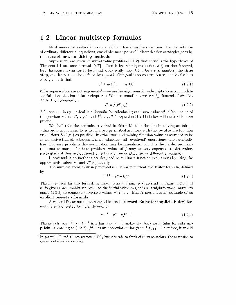
Figure ������ One step of the Euler and midpoint formulas� The solid curvesrepresent not the exact solution to the initial�value problem� but the exact solu�tion to the problem ut� f � utn�� vn�
appear that vn� cannot be determined from ������ unless it is already known� In fact� toimplement an implicit formula� one must employ an iteration of some kind to solve for theunknown vn�� and this involves extra work� not to mention the questions of existence anduniqueness�� But as we shall see� the advantage of ������ is that in some situations it maybe stable when ������ is catastrophically unstable� Throughout the numerical solution ofdi�erential equations� there is a tradeo� between explicit methods� which tend to be easierto implement� and implicit ones� which tend to be more stable� Typically this tradeo� takesthe form that an explicit method requires less work per time step� while an implicit methodis able to take larger and hence fewer time steps without sacri�cing accuracy to unstableoscillations��
An example of a more accurate linear multistep formula is the trapezoid rule�
vn� � vn k
�fn fn��� ������
also an implicit one�step formula� Another is the midpoint rule�
vn� � vn�� �kfn� ������
an explicit two�step formula Figure �����b�� The fact that ������ involves multiple timelevels raises a new di�culty� We can set v��u�� but to compute v� with this formula� where
�In so�called predictor�corrector methods not discussed in this book the iteration is terminatedbefore convergence giving a class of methods intermediate between explicit and implicit�
�But don�t listen to people who talk about conservation of di�culty� as if there were never anyclear winners� We shall see that sometimes explicit methods are vastly more e�cient than implicitones �large non�sti� systems of ODEs� and sometimes it is the reverse �small sti� systems��

���� LINEAR MULTISTEP FORMULAS TREFETHEN ���� � �
shall we get v��� Or if we want to begin by computing v�� where shall we get v�� Thisinitialization problem is a general one for linear multistep formulas� and it can be addressedin several ways� One is to calculate the missing values numerically by some simpler formulasuch as Euler�s method�possibly applied several times with a smaller value of k to avoidloss of accuracy� Another is to handle the initialization process by Runge�Kutta methods�to be discussed in Section ����
In Chapter � we shall see that the formulas ������ ������ have important analogs for
partial di�erential equations�y For the easier problems of ordinary di�erential equations�however� they are too primitive for most purposes� Instead one usually turns to morecomplicated and more accurate formulas� such as the fourth�order Adams�Bashforthformula�
vn� � vn k
��
���fn���fn�� �!fn����fn��
�� ����!�
an explicit four�step formula� or the fourth�order Adams�Moulton formula�
vn� � vn k
��
��fn� ��fn��fn�� fn��
�� ������
an implicit three�step formula� Another implicit three�step formula is the third�orderbackwards dierentiation formula�
vn� � ����v
n� ��v
n�� ���v
n�� ���kf
n�� ������
whose advantageous stability properties will be discussed in Section ����
EXAMPLE ������ Let us perform an experiment to compare some of these methods� Theinitial�value problem will be
ut�u� t� ����� u�� �� ������
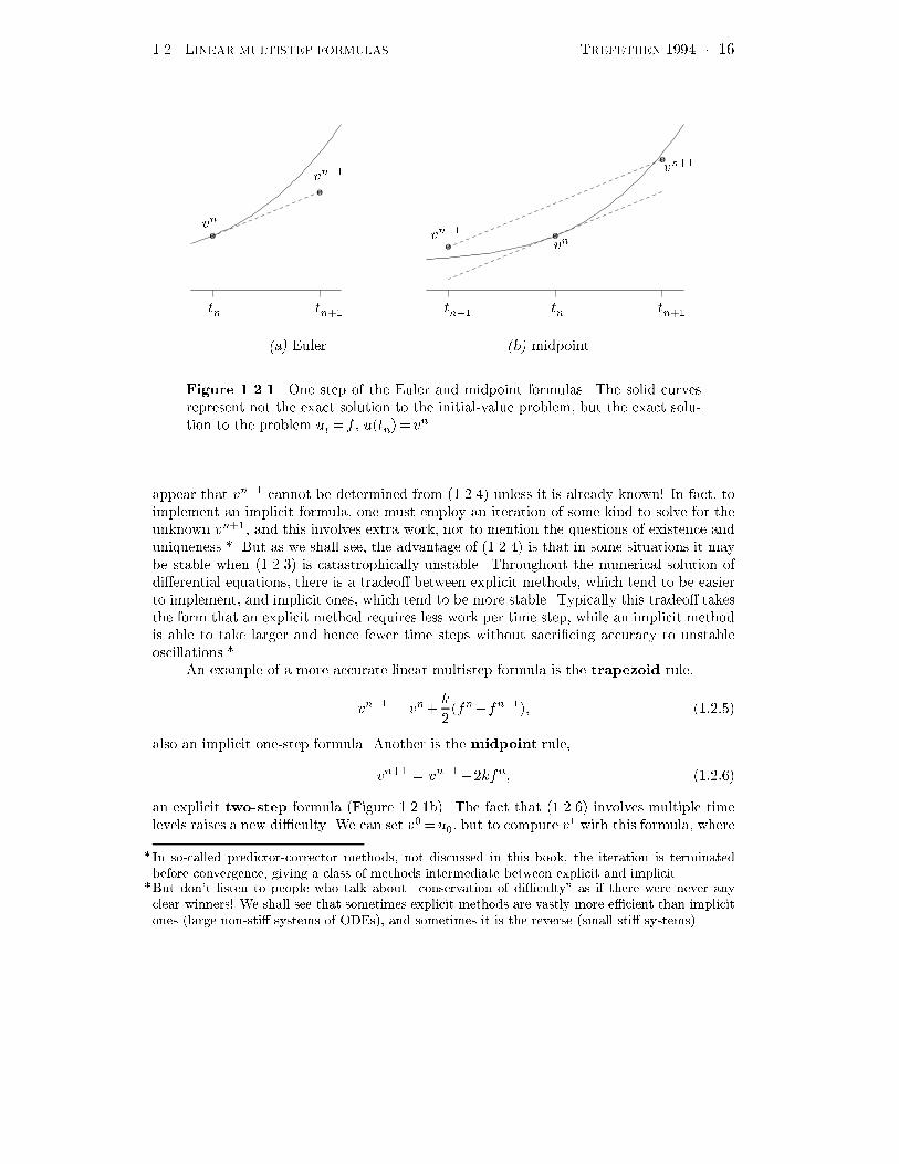
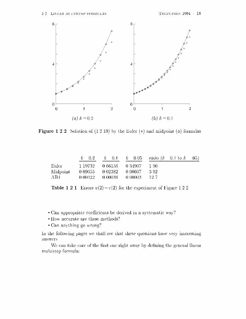
whose solution is simply ut� � et� Figure ����� compares the exact solution with the nu�merical solutions obtained by the Euler and midpoint formulas with k � �� and k � ���For simplicity� we took v� equal to the exact value ut�� to start the midpoint formula��A solution with the fourth�order Adams�Bashforth formula was also calculated� but is in�distinguishable from the exact solution in the plot� Notice that the midpoint formula doesmuch better than the Euler formula� and that cutting k in half improves both� To makethis precise� Table ����� compares the various errors u���v��� The �nal column of ratiossuggests that the errors for the three formulas have magnitudes "k�� "k��� and "k�� ask� � The latter �gure accounts for the name �fourth�order�� see the next section�
Up to this point we have listed a few formulas� some with rather compli�cated coe�cients� and shown that they work at least for one problem� Fortu�nately� the subject of linear multistep methods has a great deal more order init than this� A number of questions suggest themselves�
�What is the general form of a linear multistep method!
yEuler Backward Euler Crank�Nicolson and Leap Frog�
���� LINEAR MULTISTEP FORMULAS TREFETHEN ���� � ��
**
**
**
*
*
*
*
*
oo
oo
o
o
o
o
o
o
o
* * * * * * * **
**
**
**
**
*
*
*
*
o o o o o o oo
oo
oo
oo
oo
o
o
o
o
o
� � ��
�
�
� � ��
�
�
�a� k���� �b� k����
Figure ������ Solution of ������� by the Euler �� and midpoint o� formulas�
k���� k���� k����� ratio k���� to k� ����
Euler ������� ������� ������� ����Midpoint ������� ������ ������� ����AB� ������� ������ ������� ����
Table ������ Errors u ���v �� for the experiment of Figure ������
� Can appropriate coe�cients be derived in a systematic way!� How accurate are these methods!� Can anything go wrong!
In the following pages we shall see that these questions have very interestinganswers�
We can take care of the �rst one right away by de�ning the general linearmultistep formula�
���� LINEAR MULTISTEP FORMULAS TREFETHEN ���� � ��
An s�step linear multistep formula is a formula
sXj�
�jvn�j � k
sXj�
�jfn�j �������
for some constants f�jg and f�jg with �s�� and either � �� or � ���If �s�� the formula is explicit� and if �s �� it is implicit�
Readers familiar with electrical engineering may notice that ������� lookslike the de�nition of a recursive or IIR digital �lter Oppenheim Schafer������ Linear multistep formulas can indeed be thought of in this way� andmany of the issues to be described here also come up in digital signal process�ing� such as the problem of stability and the idea of testing for it by looking forzeros of a polynomial in the unit disk of the complex plane� A linear multistepformula is not quite a digital �lter of the usual kind� however� In one respectit is more general� since the function f depends on u and t rather than on talone� In another respect it is more narrow� since the coe�cients are chosenso that the formula has the eect of integration� Digital �lters are designedto accomplish a much wider variety of tasks� such as high�pass or low�pass�ltering � smoothing�� dierentiation� or channel equalization�
What about the word �linear�! Do linear multistep formulas apply onlyto linear dierential equations! Certainly not� Equation ������� is calledlinear because the quantities vn and fn are related linearly� f may very wellbe a nonlinear function of u and t� Some authors refer simply to �multistepformulas� to avoid this potential source of confusion�
EXERCISES
� ������ What are s� f�jg� and fjg for formulas ����!� �������
� ������ Linear multistep formula for a system of equations� One of the footnotes aboveclaimed that the extension of linear multistep methods to systems of equations is easy�Verify this by writing down exactly what the ��� system of Example ����� becomes whenit is approximated by the midpoint rule �������
� ������ Exact answers for low�degree polynomials� If L is a nonnegative integer� the initial�value problem
utt��L
t �ut�� u�� �
has the unique solution ut� � t ��L� Suppose we calculate an approximation v�� by alinear multistep formula� using exact values where necessary for the initialization�
�a� For which L does ������ reproduce the exact solution� �b� ������� �c� ����!��
� ����� Extrapolation methods�

���� LINEAR MULTISTEP FORMULAS TREFETHEN ���� � ��
�a� The values Vk � v�� � u�� computed by Euler�s method in Figure ����� are V��� ���!�!� and V���� �����!�� Use a calculator to compute the analogous value V����
�b� It can be shown that these quantities Vk satisfy
Vk � u�� C�k C�k� Ok��
for some constants C�� C� as k� � In the process known as Richardson extrapola�tion� one constructs the higher�order estimates
V �
k � Vk Vk�V�k� � u�� Ok��
andV ��
k � V �
k �� V
�
k�V �
�k� � u�� Ok���
Apply these formulas to compute V ��
��� for this problem� How accurate is it� This isan example of an extrapolation method for solving an ordinary di�erential equationGragg ����� Bulirsch # Stoer ������ The analogous method for calculating integralsis known as Romberg integration Davis # Rabinowitz ��!���

���� ACCURACY AND CONSISTENCY TREFETHEN ���� � ��
���� Accuracy and consistency
In this section we de�ne the consistency and order of accuracy of a linear multistep for�mula� as well as the associated characteristic polynomials z� and �z�� and show how thesede�nitions can be applied to derive accurate formulas by a method of undetermined coe��cients� We also show that linear multistep formulas are connected with the approximationof the function logz by the rational function z���z� at z���
With f�jg and fjg as in �������� the characteristic polynomials or generatingpolynomials� for the linear multistep formula are de�ned by
z��
sXj �
�jzj � �z��
sXj �
jzj � ������
The polynomial has degree exactly s� and � has degree s if the formula is implicit or �sif it is explicit� Specifying and � is obviously equivalent to specifying the linear multistepformula by its coe�cients� We shall see that and � are convenient for analyzing accuracyand indispensable for analyzing stability�
EXAMPLE ������ Here are the characteristic polynomials for the �rst four formulas ofthe last section�
Euler ������� s��� z�� z��� �z�� ��
Backward Euler ������� s��� z�� z��� �z�� z�
Trapezoid ������� s��� z�� z��� �z�� �� z ���
Midpoint ������� s��� z�� z���� �z�� �z�
Now let Z denote a time shift operator that acts both on discretefunctions according to
Zvn� vn��� ������
and on continuous functions according to
Zu t�� u t�k�� ������
In principle we should write �Zv�n and �Zu� t�� but expressions like Zvn andeven Z vn� are irresistibly convenient�� The powers of Z have the obviousmeanings� e�g�� Z�vn� vn�� and Z��u t�� u t�k��
Equation ������� can be rewritten compactly in terms of Z� � and �
Z�vn�k Z�fn � �� ������
When a linear multistep formula is applied to solve an ODE� this equation issatis�ed exactly since it is the de�nition of the numerical approximation fvng�

���� ACCURACY AND CONSISTENCY TREFETHEN ���� � ��
If the linear multistep formula is a good one� the analogous equation oughtto be nearly satis�ed when fvng and ffng are replaced by discretizations ofany well�behaved function u t� and its derivative ut t�� With this in mind� letus de�ne the linear multistep di�erence operator L� acting on the set ofcontinuously dierentiable functions u t�� by
L � Z��kD Z�� ������
where D is the time dierentiation operator� that is�
Lu tn� � Z�u tn��k Z�ut tn�
�sX
j�
�ju tn�j��ksX
j�
�jut tn�j�� ������
If the linear multistep formula is accurate� Lu tn� ought to be small� and wemake this precise as follows� Let a function u t� and its derivative ut t� beexpanded formally in Taylor series about tn�
u tn�j� � u tn��jkut tn���� jk�
�utt tn�� � � � � ������
ut tn�j� � ut tn��jkutt tn���� jk�
�uttt tn�� � � � � �����
Inserting these formulas in ������ gives the formal local discretization
error or formal local truncation error� for the linear multistep formula�
Lu tn� � Cu tn��C�kut tn��C�k�utt tn�� � � � � ������
where
C � �� � � ���s�
C� � ������� � � ��s�s�� �� � � ���s��
C� ��� ������� � � ��s
��s�� ������� � � ��s�s����
Cm �sX
j�
jm
m"�j�
sXj�
jm��
m���"�j � �������
We now de�ne�
A linear multistep formula has order of accuracy p if
Lu tn� � # kp��� as k ��
i�e�� if C �C� � � � ��Cp� � but Cp�� � �� The error constant is Cp���The formula is consistent if C �C� � �� i�e�� if it has order of accuracyp� ��

���� ACCURACY AND CONSISTENCY TREFETHEN ���� � ��
EXAMPLE ����� CONTINUED� First let us analyze the local accuracy of the Eulerformula in a lowbrow fashion that is equivalent to the de�nition above� we suppose thatv�� � � � �vn are exactly equal to ut��� � � � �utn�� and ask how close vn� will then be to utn���If vn�utn� exactly� then by de�nition�
vn� � vn kfn � utn� kuttn��
while the Taylor series ����!� gives
utn�� � utn� kuttn� k�
�utttn� Ok���
Subtraction gives
utn���vn� �k�
�utttn� Ok��
as the formal local discretization error of the Euler formula�Now let us restate the argument in terms of the operator L� By combining ������
and ����!�� or by calculating C��C��� C���� � C��
�� from the values ������ �����
���� �� in ������� we obtain
Lutn� � utn���utn��kuttn�
�k�
�utttn�
k�
�uttttn� � � � � �������
Thus again we see that the order of accuracy is �� and evidently the error constant is �� �
Similarly� the trapezoid rule ������ has
Lutn� � utn���utn��k
�
�uttn�� uttn�
�� �k�
��uttttn��
k�
��utttttn� � � � � �������
with order of accuracy � and error constant � ��� � and the midpoint rule ������ has
Lutn� � ��k
�uttttn� ��k
�utttttn� � � � � �������
with order of accuracy � and error constant �� �
The idea behind the de�nition of order of accuracy is as follows� Equation ������ suggests that if a linear multistep formula is applied to a problem with a
su�ciently smooth solution u t�� an error of approximately Cp��kp�� dp�u
dtp� tn�
�O kp��� will be introduced locally at step n�� This error is known as thelocal discretization or truncation� error at step n for the given initial�value problem as opposed to the formal local discretization error� which is a
�As usual the limit associated with the Big�O symbol �k� � is omitted here because it is obvious�

���� ACCURACY AND CONSISTENCY TREFETHEN ���� � ��
formal expression that does not depend on the initial�value problem�� Sincethere are T�k �# k��� steps in the interval ���T �� these local errors can beexpected to add up to a global error O kp�� We shall make this argumentmore precise in Section ����
With hindsight� it is obvious by symmetry that the trapezoid and mid�point formulas had to have even orders of accuracy� Notice that in ������� theterms involving vn�j are antisymmetric about tn� and those involving fn�j
are symmetric� In ������� the eect of these symmetries is disguised� becausetn�� was shifted to tn for simplicity of the formulas in passing from ������ to ������� and ������� However� if we had expressed Lu tn� as a Taylor seriesabout tn�� instead� we would have obtained
Lu tn� ���k
�uttt tn������k
�uttttt tn����O k���
with all the even�order derivatives in the series vanishing due to symmetry�Now it can be shown that to leading order� it doesn�t matter what point oneexpands Lu tn� about� C� � � � �Cp�� are independent of this point� though thesubsequent coe�cients Cp���Cp��� � � � are not� Thus the vanishing of the even�order terms above is a valid explanation of the second�order accuracy of themidpoint formula� For the trapezoid rule ������� we can make an analogousargument involving an expansion of Lu tn� about tn�����
As a rule� symmetry arguments do not go very far in the analysis ofdiscrete methods for ODEs� since most of the formulas used in practice are ofhigh order and fairly complicated� They go somewhat further with the simplerformulas used for PDEs�
The de�nition of order of accuracy suggests amethod of undetermined
coe�cients for deriving linear multistep formulas� having decided somehowwhich �j and �j are permitted to be nonzero� simply adjust these parametersto make p as large as possible� If there are q parameters� not counting the�xed value �s��� then the equations ������� with ��m� q�� constitute aq�q linear system of equations� If this system is nonsingular� as it usually is�it must have a unique solution that de�nes a linear multistep formula of orderat least p� q��� See Exercise ������
The method of undetermined coe�cients can also be described in another�equivalent way that was hinted at in Exercise ������ It can be shown that anyconsistent linear multistep formula computes the solution to an initial�valueproblem exactly in the special case when that solution is a polynomial p t�of degree L� provided that L is small enough� The order of accuracy p is thelargest such L see Exercise ������� To derive a linear multistep formula for aparticular choice of available parameters �j and �j � one can choose the param�eters in such a way as to make the formula exact when applied to polynomialsof as high a degree as possible�

���� ACCURACY AND CONSISTENCY TREFETHEN ���� � ��
At this point it may appear to the reader that the construction of linearmultistep formulas is a rather uninteresting matter� Given s� �� why not sim�ply pick �� � � � ��s�� and �� � � � ��s so as to achieve order of accuracy �s! Theanswer is that for s� �� the resulting formulas are unstable and consequentlyuseless see Exercise ������� In fact� as we shall see in Section ���� a famoustheorem of Dahlquist asserts that a stable s�step linear multistep formula canhave order of accuracy at most s��� Consequently� nothing can be gained bypermitting all �s�� coe�cients in an s�step formula to be nonzero� Instead�the linear multistep formulas used in practice usually have most of the �j ormost of the �j equal to zero� In the next section we shall describe severalimportant families of this kind�
And there is another reason why the construction of linear multistep for�mulas is interesting� It can be made exceedingly slick" We shall now describehow the formulas above can be analyzed more compactly� and the question oforder of accuracy reduced to a question of rational approximation� by manip�ulation of formal power series�
Taking j �� in ������ gives the identity
u tn��� � u tn��kut tn����k
�utt tn�� � � � �
Since u tn����Zu tn�� here is another way to express the same fact�
Z � �� kD�� ��� kD�
�� ��� kD�
�� � � � � ekD � �������
Like ������� this formula is to be interpreted as a formal identity� the ideais to use it as a tool for manipulation of terms of series without making anyclaims about convergence� Inserting ������� in ������ and comparing with ������ gives
L � ekD ��kD ekD � � C�C� kD��C� kD��� � � � � �������
In other words� the coe�cients Cj of ������ are nothing else than the Taylor
series coe�cients of the function ekD ��kD ekD � with respect to the argu�ment kD� If we let � be an abbreviation for kD� this equation becomes evensimpler�
L � e���� e�� � C�C���C���� � � � � �������
With the aid of a symbolic algebra system such as Macsyma� Maple� or Mathe�matica� it is a trivial matter to make use of ������� to compute the coe�cientsCj for a linear multistep formula if the parameters �j and �j are given� SeeExercise ������
By de�nition� a linear multistep formula has order of accuracy p if andonly if the the term between the equal signs in ������� is # �p��� as � ��
���� ACCURACY AND CONSISTENCY TREFETHEN ���� � �
Since e�� is an analytic function of �� if it is nonzero at ��� we can dividethrough to conclude that the linear multistep formula has order of accuracy pif and only if
e��
e��� ��# �p��� as � �� �������
The following theorem restates this conclusion in terms of the variable z� e��
LINEAR MULTISTEP FORMULAS AND RATIONAL APPROXIMATION
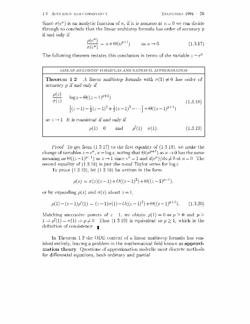
Theorem ���� A linear multistep formula with �� � � has order ofaccuracy p if and only if
z�
z�� logz�# z���p���
�h z���� �
� z����� �
� z������� �
i�# z���p���
������
as z �� It is consistent if and only if
��� � and � ��� ��� �������
Proof� To get from ������� to the �rst equality of ������� we make thechange of variables z� e�� �� logz� noting that # �p��� as � � has the samemeaning as # z���p��� as z � since e��� and d e���d� �� at ���� Thesecond equality of ������ is just the usual Taylor series for logz�
To prove �������� let ������ be written in the form
z� � z� z����O z������# z���p����
or by expanding z� and z� about z���
��� z���� �� � z��� ���O z������# z���p���� �������
Matching successive powers of z� �� we obtain �� � �� p � � and p ��� � �� � ��� p � �� Thus ������� is equivalent to p� �� which is thede�nition of consistency�
In Theorem ��� the ODE context of a linear multistep formula has van�ished entirely� leaving a problem in the mathematical �eld known as approxi�mation theory� Questions of approximation underlie most discrete methodsfor dierential equations� both ordinary and partial�
���� ACCURACY AND CONSISTENCY TREFETHEN ���� � �
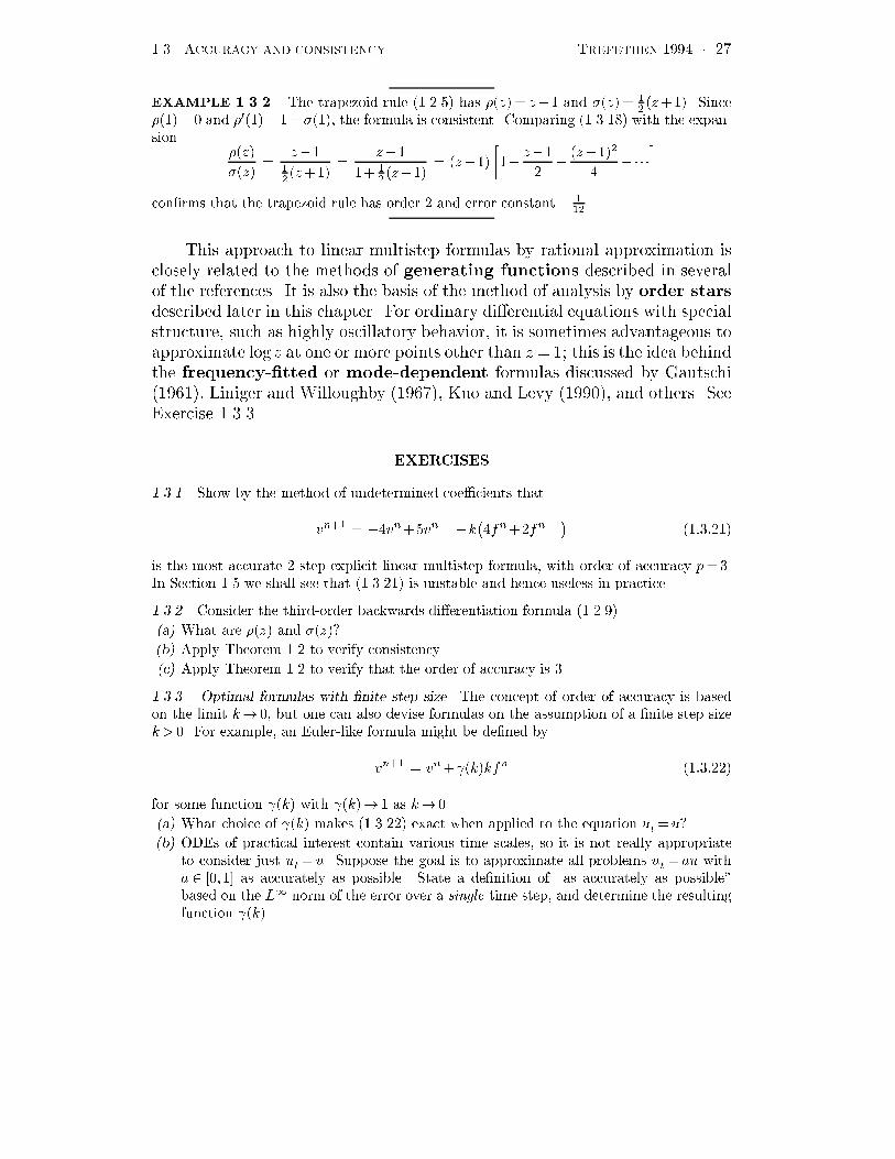
EXAMPLE ������ The trapezoid rule ������ has z� � z�� and �z� � �� z ��� Since
��� and ���� ������ the formula is consistent� Comparing ������� with the expan�sion
z�
�z��
z���� z ��
�z��
� �� z���
� z���
��� z��
�
z����
���� �
�
con�rms that the trapezoid rule has order � and error constant � ��� �
This approach to linear multistep formulas by rational approximation isclosely related to the methods of generating functions described in severalof the references� It is also the basis of the method of analysis by order starsdescribed later in this chapter� For ordinary dierential equations with specialstructure� such as highly oscillatory behavior� it is sometimes advantageous toapproximate logz at one or more points other than z��� this is the idea behindthe frequency��tted or mode�dependent formulas discussed by Gautschi ������ Liniger and Willoughby ������ Kuo and Levy ������ and others� SeeExercise ������
EXERCISES
� ������ Show by the method of undetermined coe�cients that
vn� � ��vn �vn�� k��fn �fn��
��������
is the most accurate ��step explicit linear multistep formula� with order of accuracy p���In Section ��� we shall see that ������� is unstable and hence useless in practice�
� ������ Consider the third�order backwards di�erentiation formula �������
�a� What are z� and �z��
�b� Apply Theorem ��� to verify consistency�
�c� Apply Theorem ��� to verify that the order of accuracy is ��
� ������ Optimal formulas with �nite step size� The concept of order of accuracy is basedon the limit k� � but one can also devise formulas on the assumption of a �nite step sizek � � For example� an Euler�like formula might be de�ned by
vn� � vn �k�kfn �������
for some function �k� with �k�� � as k� �
�a� What choice of �k� makes ������� exact when applied to the equation ut�u�
�b� ODEs of practical interest contain various time scales� so it is not really appropriateto consider just ut� u� Suppose the goal is to approximate all problems ut� au witha � ���� as accurately as possible� State a de�nition of �as accurately as possible�based on the L� norm of the error over a single time step� and determine the resultingfunction �k��
���� ACCURACY AND CONSISTENCY TREFETHEN ���� � ��
������� ����� Numerical experiments� Consider the scalar initial�value problem
utt�� ecos�tu�t�� for t� ����� u�� �
In this problem you will test four numerical methods� i� Euler� ii� Midpoint� iii� Fourth�order Adams�Bashforth� and iv� Fourth�order Runge�Kutta� de�ned by
a �� kfvn� tn��
b �� kfvn a��� tn k����
c �� kfvn b��� tn k����
d �� kfvn c� tn k��
vn� �� vn �� a �b �c d� �
�������
�a� Write a computer program to implement ������� in high precision arithmetic �� digitsor more�� Run it with k����� ���� � � � until you are con�dent that you have a computedvalue v�� accurate to at least � digits� This will serve as your �exact solution�� Makea computer plot or a sketch of vt�� Store appropriate values from your Runge�Kuttacomputations for use as starting values for the multistep formulas ii� and iii��
�b� Modify your program so that it computes v�� by each of the methods i� iv� for thesequence of time steps k��������� � � � ������� Make a table listing v�� and v���u��for each method and each k�
�c� Draw a plot on a log�log scale of four curves representing jv���u��j as a function ofthe number of evaluations of f � for each of the four methods� Make sure you calculateeach fn only once� and count the number of function evaluations for the Runge�Kuttaformula rather than the number of time steps��
�d� What are the approximate slopes of the lines in c�� and why� If you can�t explainthem� there may be a bug in your program�very likely in the speci�cation of initialconditions�� Which of the four methods is most e�cient�
�e� If you are programming in Matlab� solve this same problem with the programs ode��and ode�� with eight or ten di�erent error tolerances� Measure how many time stepsare required for each run and how much accuracy is achieved in the value u��� and addthese new results to your plot of c�� What are the observed orders of accuracy of theseadaptive codes� How do they compare in e�ciency with your non�adaptive methodsi� iv��
� ����� Statistical e�ects It was stated above that if local errors of magnitude Okp�� aremade at each of "k��� steps� then the global error will have magnitude Okp�� However�one might argue that more likely� the local errors will behave like random numbers oforder Okp��� and will accumulate in a square�root fashion according to the principles ofa random walk� giving a smaller global error Okp����� Experiments show that for mostproblems� including those of Example ����� and Exercise ������ this optimistic prediction isinvalid� What is the fallacy in the random walk argument� Be speci�c� citing an equationin the text to support your answer�
� ������ Prove the lemma alluded to on p� ��� An s�step linear multistep formula has order ofaccuracy p if and only if� when applied to an ordinary di�erential equation ut� qt�� it givesexact results whenever q is a polynomial of degree p� but not whenever q is a polynomial

���� ACCURACY AND CONSISTENCY TREFETHEN ���� � ��
of degree p �� Assume arbitrary continuous initial data u� and exact numerical initialdata v�� � � � �v
s����
� ������ If you have access to a symbolic computation system� carry out the suggestion onp� ��� write a short program which� given the parameters �j and j for a linear multistepformula� computes the coe�cients C��C�� � � �� Use your program to verify the results ofExercises ����� and ������ and then explore other linear multistep formulas that interestyou�

���� DERIVATION OF LINEAR MULTISTEP FORMULAS TREFETHEN ���� � ��
���� Derivation of linear multistep formulas
The oldest linear multistep formulas are the Adams formulas�
vns�vns�� � k
sXj �
jfnj � ������
which date to the work of J� C� Adams� as early as ����� In the notation of ������� wehave �s � �� �s�� ���� and �� � � � � � �s�� � � and the �rst characteristic polynomialis z� � zs�zs��� For each s� �� the s�step Adams�Bashforth and Adams�Moultonformulas are the optimal explicit and implicit formulas of this form� respectively� �Optimal�means that the available coe�cients fjg are chosen to maximize the order of accuracy� andin both Adams cases� this choice turns out to be unique�
We have already seen the ��step Adams�Bashforth and Adams�Moulton formulas� theyare Euler�s formula ������ and the trapezoid formula ������� respectively� The fourth�orderAdams�Bashforth and Adams�Moulton formulas� with s� � and s� �� respectively� werelisted above as ����!� and ������� The coe�cients of these and other formulas are listed inTables ����� ����� on the next page� The �stencils� of various families of linear multistepformulas are summarized in Figure ������ which should be self�explanatory�
To calculate the coe�cients of Adams formulas� there is a simpler and more enlight�ening alternative to the method of undetermined coe�cients mentioned in the last section�Think of the values fn� � � � �fns�� A�B� or fn� � � � �fns A�M� as discrete samples of acontinuous function ft�� fut�� t� that we want to integrate�
utns��utns��� �
Z tn�s
tn�s��
utt�dt �
Z tn�s
tn�s��
ft�dt�
as illustrated in Figure �����a� Of course fn� � � � �fns will themselves be inexact due toearlier errors in the computation� but we ignore this for the moment�� Let qt� be the uniquepolynomial of degree at most s�� A�B� or s A�M� that interpolates these data� and set
vns�vns�� �
Z tn�s
tn�s��
qt�dt� ������
Since the integral is a linear function of the data ffnjg� with coe�cients that can becomputed once and for all� ������ implicitly de�nes a linear multistep formula of the Adamstype �������
EXAMPLE ������ Let us derive the coe�cients of the �nd�order Adams�Bashforth for�mula� which are listed in Table ������ In this case the data to be interpolated are fn and
�the same Adams who �rst predicted the existence of the planet Neptune

���� DERIVATION OF LINEAR MULTISTEP FORMULAS TREFETHEN ���� � ��
Adams� Adams� Generalized BackwardsBashforth Moulton Nystr�om Milne�Simpson Di erentiation
�j �j �j �j �j �j �j �j �j �j j
� � � � � � � � n�s
� � � � � � � n�s��
� � � � � � � n�s�����
������
������
���
� � � � � n
Figure ������ Stencils of various families of linear multistep formulas�
numberof steps s order p �s �s�� �s�� �s�� �s��
� � � � �EULER�
� � � �� ��
�
� � � ���� ���
����
� � � �� �
������ �
��
Table ������ Coe�cients f�jg of Adams�Bashforth formulas�
numberof steps s order p �s �s�� �s�� �s�� �s��
� � � �BACKWARD EULER�
� � ��
�� �TRAPEZOID�
� � ��
��� � �
��
� � ��
��� �
�����
� � ����
����� ����
�� � ��� � �
��
Table ������ Coe�cients f�jg of Adams�Moulton formulas�
numberof steps s order p �s �s�� �s�� �s�� �s�� �s
� � � �� �BACKWARD EULER� �
� � � ���
��
��
� � � �����
�� � �
�����
� � � ����
��� ���
���
���
Table ������ Coe�cients f�jg and �s of backwards di erentiation formulas�

���� DERIVATION OF LINEAR MULTISTEP FORMULAS TREFETHEN ���� � ��
fn�� and the interpolant is the linear polynomial qt� � fn��k��fn��fn�tn�� t��Therefore ������ becomes
vn��vn� �
Z tn��
tn��
�fn��k��fn��fn�tn��t�
�dt
� kfn��k��fn��fn�
Z tn��
tn��
tn��t�dt
� kfn��k��fn��fn�� ��k
��
��
�kfn�� �
�kfn� ������
o
o
oo
o
*
*
**
* o
o
oo
o
*
*
**
*fn
fn�s��
fn�s
tn�s�� tn�s
vn
vn�s
tn�s
�
q t�
�
q t�
a� Adams b� backwards dierentiation
Figure ����� Derivation of Adams and backwards dierentiationformulas via polynomial interpolation�
More generally� the coe�cients of the interpolating polynomial q can bedetermined with the aid of the Newton interpolation formula� To beginwith� consider the problem of interpolating a discrete function fyng in thepoints �� � � � �� by a polynomial q t� of degree at most �� Let $ and r denotethe forward and backward di�erence operators
$ � Z��� r � ��Z��� ������
where � represents the identity operator� For example�
$yn � yn���yn� $�yn � yn����yn���yn�
Also� let�aj
�denote the binomial coe�cient �a choose j��
�a
j
��
a a��� a��� � � � a�j���
j"� ������
���� DERIVATION OF LINEAR MULTISTEP FORMULAS TREFETHEN ���� � ��
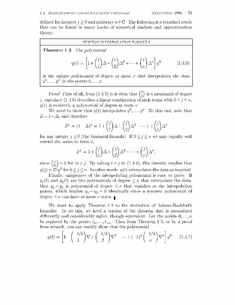
de�ned for integers j� � and arbitrary a� C � The following is a standard resultthat can be found in many books of numerical analysis and approximationtheory�
NEWTON INTERPOLATION FORMULA
Theorem ���� The polynomial
q t� �
��
�t
�
�$�
�t
�
�$�� � � ��
�t
�
�$�
y ������
is the unique polynomial of degree at most � that interpolates the datay� � � � �y� in the points �� � � � ���
Proof� First of all� from ������ it is clear that�tj
�is a monomial of degree
j� and since ������ describes a linear combination of such terms with �� j� ��q t� is evidently a polynomial of degree at most ��
We need to show that q t� interpolates y� � � � �y�� To this end� note thatZ ���$� and therefore
Zj � ��$�j � ��
�j
�
�$�
�j
�
�$�� � � ���
�j
j
�$j
for any integer j� � the binomial formula�� If �� j� � we may equally wellextend the series to term ��
Zj � ��
�j
�
�$�
�j
�
�$�� � � ��
�j
�
�$� �
since�jm
��� for m�j� By taking t� j in ������� this identity implies that
q j��Zjy for �� j� �� In other words� q t� interpolates the data as required�Finally� uniqueness of the interpolating polynomial is easy to prove� If
q� t� and q� t� are two polynomials of degree � � that interpolate the data�then q�� q� is polynomial of degree � � that vanishes at the interpolationpoints� which implies q�� q� � � identically since a nonzero polynomial ofdegree � � can have at most � zeros�
We want to apply Theorem ��� to the derivation of Adams�Bashforthformulas� To do this� we need a version of the theorem that is normalizeddierently and considerably uglier� though equivalent� Let the points �� � � � ��be replaced by the points t� � � � � t�� � Then from Theorem ���� or by a prooffrom scratch� one can readily show that the polynomial
q t� �
��
��t�k
�
�r�
��t�k
�
�r���� �� ����
��t�k
�
�r�
y ������

���� DERIVATION OF LINEAR MULTISTEP FORMULAS TREFETHEN ���� � ��
is the unique polynomial of degree at most � that interpolates the data y��� � � � �y in the points t�� � � � � � t� Note that among other changes� $ has beenreplaced by r�
Now let us replace y by f � � by s��� and t by t�tn�s��� hence t��� � � � � tby tn� � � � � tn�s��� Equation ������ then becomes
q t� �
��
� tn�s���t��k
�
�r� � � �� ���s��
� tn�s���t��k
s��
�rs��
fn�s���
�����Inserting this expression in ������ gives
vn�s�vn�s�� � ks��Xj�
jrjfn�s���
where
j � ���j
k
Z tns
tns��
� tn�s���t��k
j
�dt � ���j
Z �
���
j
�d��
The �rst few values j are
��� ���
�� ��
����
�����
���
�� ��
���
��� ��
���
����� ������
���
��� ��
��
���� ��
�����
�������
The following theorem summarizes this derivation and some related facts�
���� DERIVATION OF LINEAR MULTISTEP FORMULAS TREFETHEN ���� � ��
ADAMS�BASHFORTH FORMULAS
Theorem ��� For any s � �� the s�step Adams�Bashforth formula hasorder of accuracy s� and is given by
vn�s � vn�s���ks��Xj�
jrjfn�s��� j � ���
jZ �
���
j
�d�� �������
For j� �� the coe�cients j satisfy the recurrence relation
j��
� j���
�
� j��� � � ��
�
j�� � �� �������
Proof� We have already shown above that the coe�cients ������� corre�spond to the linear multistep formula based on polynomial interpolation� Toprove the theorem� we must show three things more� that the order of accu�racy is as high as possible� so that these are indeed Adams�Bashforth formulas�that the order of accuracy is s� and that ������� holds�
The �rst claim follows from the lemma stated in Exercise ������ If f u�t�is a polynomial in t of degree � s� then q t�� f u�t� in our derivation above� sothe formula ������ gives exact results and its order of accuracy is accordingly� s� On the other hand any other linear multistep formula with dierentcoe�cients would fail to integrate q exactly� since polynomial interpolants areunique� and accordingly would have order of accuracy � s� Thus ������� isindeed the Adams�Bashforth formula�
The second claim can also be based on Exercise ������ If the s�step Adams�Bashforth formula had order of accuracy �s� it would be exact for any problemut� q t� with q t� equal to a polynomial of degree s��� But there are nonzeropolynomials of this degree that interpolate the values f � � � �� f s � �� fromwhich we can readily derive counterexamples in the form of initial�value prob�lems with v ts���� � but u ts��� ���
Finally� for a derivation of �������� the reader is referred to Henrici �����or Hairer� N�rsett Wanner �����
EXAMPLE ������ CONTINUED� To rederive the �nd�order Adams�Bashforth formuladirectly from ������� we calculate
vn� � vn� k��fn� k��f
n��fn� � vn� k���f
n�� ��f
n��
EXAMPLE ������ To obtain the third�order Adams�Bashforth formula� we increment n
���� DERIVATION OF LINEAR MULTISTEP FORMULAS TREFETHEN ���� � �
to n � in the formula above and then add one more term k��r�fn� to get
vn� � vn� k���f
n�� ��f
n�� �
��k�fn���fn� fn
�� vn� k
�����f
n�� ����f
n� ���f
n��
which con�rms the result listed in Table ������
For Adams�Moulton formulas the derivation is entirely analogous� Wehave
vn�s�vn�s�� � ksX
j�
�j rjfn�s�
where
�j � ���j
k
Z tns
tns��
� tn�s�t��k
j
�dt � ���j
Z
��
���
j
�d��
and the �rst few values �j are
� ���� �� ���
��� �� ��
��
�����
�� ���
�� �� ��
��
��� �� ��
��
������ �������
�� ���
��� �� ��
�
��� �� ��
�����
�������
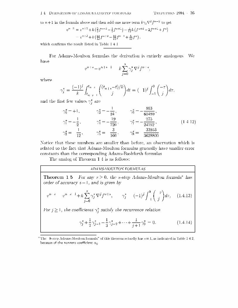
Notice that these numbers are smaller than before� an observation which isrelated to the fact that Adams�Moulton formulas generally have smaller errorconstants than the corresponding Adams�Bashforth formulas�
The analog of Theorem ��� is as follows�
ADAMS�MOULTON FORMULAS
Theorem ���� For any s � �� the s�step Adams�Moulton formula� hasorder of accuracy s��� and is given by
vn�s � vn�s���ksX
j�
�j rjfn�s� �j � ���
jZ
��
���
j
�d�� �������
For j� �� the coe�cients �j satisfy the recurrence relation
�j ��
� �j���
�
� �j��� � � ��
�
j�� � � �� �������
�The �step Adams�Moulton formula� of this theorem actually has s�� as indicated in Table �����because of the nonzero coe�cient ���

���� DERIVATION OF LINEAR MULTISTEP FORMULAS TREFETHEN ���� � �
Proof� Analogous to the proof of Theorem ����
Both sets of coe�cients f jg and f �j g can readily be converted into coef�
�cients f�jg of our standard representation �������� and the results for s� �are listed above in Tables ����� and ������
Besides Adams formulas� the most important family of linear multistepformulas dates to Curtiss and Hirschfelder in ����� and is also associated withthe name of C� W� Gear� The s�step backwards di�erentiation formula
is the optimal implicit linear multistep formula with �� � � �� �s����� Anexample was given in �������� Unlike the Adams formulas� the backwards dif�ferentiation formulas allocate the free parameters to the f�jg rather than thef�jg� These formulas are �maximally implicit� in the sense that the functionf enters the calculation only at the level n��� For this reason they are thehardest to implement of all linear multistep formulas� but as we shall see inxx���%��� they are also the most stable�
To derive the coe�cients of backwards dierentiation formulas� one canagain make use of polynomial interpolation� Now� however� the data are sam�ples of v rather than of f � as suggested in Figure �����b� Let q be the uniquepolynomial of degree � s that interpolates vn� � � � �vn�s� The number vn�s isunknown� but it is natural to de�ne it implicitly by imposing the condition
qt tn�s� � fn�s� �������
Like the integral in ������� the derivative in ������� represents a linear func�tion of the data� with coe�cients that can be computed once and for all� andso this equation constitutes an implicit de�nition of a linear multistep formula�The coe�cients for s� � were listed above in Table ������
To convert this prescription into numerical coe�cients� one can againapply the Newton interpolation formula see Exercise ������� However� theproof below is a slicker one based on rational approximation and Theorem ����
BACKWARDS DIFFERENTIATION FORMULAS
Theorem �� � For any s� �� the s�step backwards di�erentiation formulahas order of accuracy s� and is given by
sXj��
�
jrjvn�s � kfn�s� �������
Note that ������� is not quite in the standard form �������� it must benormalized by dividing by the coe�cient of vn�s��
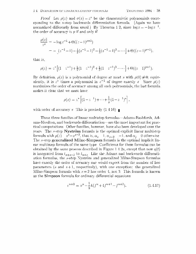
���� DERIVATION OF LINEAR MULTISTEP FORMULAS TREFETHEN ���� � ��
Proof� Let z� and z� � zs be the characteristic polynomials corre�sponding to the s�step backwards dierentiation formula� Again we havenormalized dierently from usual�� By Theorem ���� since logz �� logz���the order of accuracy is p if and only if
z�
zs� � logz���# z���p���
� �h z������ �
� z������� �
� z��������� �
i�# z���p����
that is�
z� � zsh ��z���� �
� ��z����� �� ��z����� � � �
i�# z���p����
By de�nition� z� is a polynomial of degree at most s with �� � �� equiv�alently� it is zs times a polynomial in z�� of degree exactly s� Since z�maximizes the order of accuracy among all such polynomials� the last formulamakes it clear that we must have
z� � zs� ��z���� � � ��
�
s ��z���s
��
with order of accuracy s� This is precisely ��������
These three families of linear multistep formulas�Adams�Bashforth� Ad�ams�Moulton� and backwards dierentiation�are the most important for prac�tical computations� Other families� however� have also been developed over theyears� The s�step Nystr�om formula is the optimal explicit linear multistepformula with z�� zs�zs��� that is� �s��� �s������ and �j �� otherwise�The s�step generalized Milne�Simpson formula is the optimal implicit lin�ear multistep formula of the same type� Coe�cients for these formulas can beobtained by the same process described in Figure �����a� except that now q t�is integrated from tn�s�� to tn�s� Like the Adams and backwards dierenti�ation formulas� the s�step Nystr&om and generalized Milne�Simpson formulashave exactly the order of accuracy one would expect from the number of freeparameters s and s��� respectively�� with one exception� the generalizedMilne�Simpson formula with s�� has order �� not �� This formula is knownas the Simpson formula for ordinary dierential equations�
vn�� � vn��
�k fn��fn���fn���� �������
���� DERIVATION OF LINEAR MULTISTEP FORMULAS TREFETHEN ���� � ��
EXERCISES
� ����� Second�order backwards di�erentiation formula� Derive the coe�cients of the ��stepbackwards di�erentiation formula in Table ������
�a� By the method of undetermined coe�cients�
�b� By Theorem ���� making use of the expansion z��z���� �z��� ��
�c� By interpolation� making use of Theorem ����
� ����� Backwards di�erentiation formulas� Derive ������� from Theorem ����
� ����� Third�order Nystr�om formula� Determine the coe�cients of the third�order Nystr$omformula by interpolation� making use of Theorem ����
� ���� Quadrature formulas� What happens to linear multistep formulas when the functionfu�t� is independent of u� To be speci�c� what happens to Simpson�s formula �����!��Comment on the e�ect of various strategies for initializing the point v� in an integration ofsuch a problem by Simpson�s formula�

���� STABILITY TREFETHEN ���� � ��
���� Stability
It is time to introduce one of the central themes of this book� stability� Before ���� theword stability rarely if ever appeared in papers on numerical methods� but by ���� at whichtime computers were widely distributed� its importance had become universally recognized��Problems of stability a�ect almost every numerical method for solving di�erential equations�and they must be confronted head�on�
For both ordinary and partial di�erential equations� there are two main stability ques�tions that have proved important over the years�
Stability�y If t� is held �xed� do the computed values vt� remain bounded as k� �
Eigenvalue stability� If k � is held �xed� do the computed values vt� remainbounded as t���
These two questions are related� but distinct� and each has important applications� We shallconsider the �rst in this and the following section� and the second in xx��!�����
The motivation for all discussions of stability is the most fundamental question onecould ask about a numerical method� will it give the right answer� Of course one can neverexpect exact results� so a reasonable way to make the question precise for the initial�valueproblem ������ is to ask� if t� is a �xed number� and the computation is performed withvarious step sizes k � in exact arithmetic� will vt� converge to ut� as k� �
A natural conjecture might be that for any consistent linear multistep formula� theanswer must be yes� After all� as pointed out in x���� such a method commits local errors ofsize Okp�� with p� �� and there are a total of "k��� time steps� But a simple argumentshows that this conjecture is false� Consider a linear multistep formula based purely onextrapolation of previous values fvng� such as
vn� � �vn��vn� ������
This is a �rst�order formula with z�� z���� and �z�� � and in fact we can constructextrapolation formulas of arbitrary order of accuracy by taking z� � z���s� Yet such aformula cannot possibly converge to the correct solution� for it uses no information from thedi�erential equation��
Thus local accuracy cannot be su�cient for convergence� The surprising fact is thataccuracy plus an additional condition of stability is su�cient� and necessary too� In fact thisis a rather general principle of numerical analysis� �rst formulated precisely by Dahlquist forordinary di�erential equations and by Lax and Richtmyer for partial di�erential equations�both in the ����s� Strang ����� calls it the �fundamental theorem of numerical analysis��
�See G� Dahlquist �� years of numerical instability� BIT �� ����� �������yStability is also known as zero�stability� or sometimes D�stability� for ODEs and Lax stability�or Lax�Richtmyer stability� for PDEs� Eigenvalue stability is also known as weak stability� or absolute stability� for ODEs and time�stability� practical stability� or P�stability� for PDEs�The reason for the word eigenvalue� will become apparent in xx�������
�Where exactly did the argument suggesting global errors O�kp� break down� Try to pinpoint ityourself� the answer is in the next section�
���� STABILITY TREFETHEN ���� � ��
Theorem ��� in the next section gives a precise statement for the case of linear multistepformulas� and for partial di�erential equations� see Theorem ����
We begin with a numerical experiment�
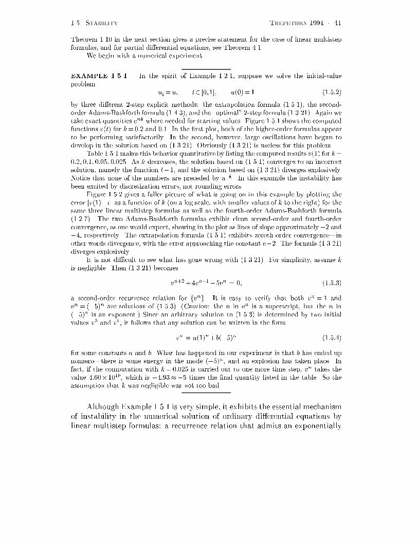
EXAMPLE ������ In the spirit of Example ������ suppose we solve the initial�valueproblem
ut�u� t� ����� u�� � ������
by three di�erent ��step explicit methods� the extrapolation formula ������� the second�order Adams�Bashforth formula ������� and the �optimal� ��step formula �������� Again wetake exact quantities enk where needed for starting values� Figure ����� shows the computedfunctions vt� for k��� and ��� In the �rst plot� both of the higher�order formulas appearto be performing satisfactorily� In the second� however� large oscillations have begun todevelop in the solution based on �������� Obviously ������� is useless for this problem�
Table ����� makes this behavior quantitative by listing the computed results v�� for k���� ��� ��� ���� As k decreases� the solution based on ������ converges to an incorrectsolution� namely the function t �� and the solution based on ������� diverges explosively�Notice that none of the numbers are preceded by a � In this example the instability hasbeen excited by discretization errors� not rounding errors�
Figure ����� gives a fuller picture of what is going on in this example by plotting theerror jv���ej as a function of k on a log scale� with smaller values of k to the right� for thesame three linear multistep formulas as well as the fourth�order Adams�Bashforth formula����!�� The two Adams�Bashforth formulas exhibit clean second�order and fourth�orderconvergence� as one would expect� showing in the plot as lines of slope approximately�� and��� respectively� The extrapolation formula ������ exhibits zeroth�order convergence�inother words divergence� with the error approaching the constant e��� The formula �������diverges explosively�
It is not di�cult to see what has gone wrong with �������� For simplicity� assume kis negligible� Then ������� becomes
vn� �vn���vn � � ������
a second�order recurrence relation for fvng� It is easy to verify that both vn � � andvn � ���n are solutions of ������� Caution� the n in vn is a superscript� but the n in���n is an exponent�� Since an arbitrary solution to ������ is determined by two initialvalues v� and v�� it follows that any solution can be written in the form
vn � a��n b���n ������
for some constants a and b� What has happened in our experiment is that b has ended upnonzero�there is some energy in the mode ���n� and an explosion has taken place� Infact� if the computation with k���� is carried out to one more time step� vn takes thevalue ������� which is �������� times the �nal quantity listed in the table� So theassumption that k was negligible was not too bad�
Although Example ����� is very simple� it exhibits the essential mechanismof instability in the numerical solution of ordinary dierential equations bylinear multistep formulas� a recurrence relation that admits an exponentially

���� STABILITY TREFETHEN ���� � ��
�� � �� �
�
�
e
�
�
e
�������
AB�
������
t t
�a� k��� �b� k���
Figure ������ Solution of ������ by three explicit two�step linear multistep for�mulas� The high�order formula ������� looks good at �rst� but becomes unstablewhen the time step is halved�
k��� k��� k��� k����
Extrapolation ������ ���!� ����!� ������ �����
�nd�order A�B ������ ����!!� ��!��� ��!���� ��!�!�
�optimal� ������� ��!���� ����!� �������� ���������
Table ������ Computed values v��� e for the initial�value problem �������
k��� ���
����
�
���
AB�
AB�
������
�������
Figure ������ Error jv���ej as a function of time step k for the solution of������ by four explicit linear multistep formulas�
���� STABILITY TREFETHEN ���� � ��
growing solution zn for some jzj � �� Such a solution is sometimes knownas a parasitic solution of the numerical method� since it is introduced bythe discretization rather than the ordinary dierential equation itself� It is ageneral principle that if such a mode exists� it will almost always be excited byeither discretization or rounding errors� or by errors in the initial conditions� Ofcourse in principle� the coe�cient b in ������ might turn out to be identicallyzero� but in practice this possibility can usually be ignored� Even if b were zeroat t��� it would soon become nonzero due to variable coe�cients� nonlinearity�or rounding errors� and the zn growth would then take over sooner or later��
The analysis of Example ����� can be generalized as follows� Given anylinear multistep formula� consider the associated recurrence relation
Z�vn �sX
j�
�jvn�j � � ������
obtained from ������ with k��� We de�ne�
A linear multistep formula is stable if all solutions fvng of the recurrencerelation ������ are bounded as n �
This means that for any function fvng that satis�es ������� there exists a con�stant M � � such that jvnj �M for all n� �� We shall refer to the recurrencerelation itself as stable� as well as the linear multistep formula�
There is an elementary criterion for determining stability of a linear mul�tistep formula� based on the characteristic polynomial �
ROOT CONDITION FOR STABILITY
Theorem ���� A linear multistep formula is stable if and only if all theroots of z� satisfy jzj � �� and any root with jzj�� is simple�
A �simple� root is a root of multiplicity ��
First proof� To prove this theorem� we need to investigate all possiblesolutions fvng� n� �� of the recurrence relation ������� Since any such solu�tion is determined by its initial values v� � � � �vs��� the set of all of them is a
�A general observation is that when any linear process admits an exponentially growing solution intheory that growth will almost invariably appear in practice� Only in nonlinear situations can theexistence of exponentially growing modes fail to make itself felt� A somewhat far��ung examplecomes from numerical linear algebra� In the solution of an N�N matrix problems by Gaussianelimination with partial pivoting�a highly nonlinear process�an explosion of rounding errors atthe rate �N�� can occur in principle but almost never does in practice �Trefethen � Schreiber Average�case stability of Gaussian elimination� SIAM J Matrix Anal Applics �����
���� STABILITY TREFETHEN ���� � ��
vector space of dimension s� Therefore if we can �nd s linearly independentsolutions vn� these will form a basis of the space of all possible solutions� andthe recurrence relation will be stable if and only if each of the basis solutionsis bounded as n �
It is easy to verify that if z is any root of z�� then
vn� zn ������
is one solution of ������� Again� on the left n is a superscript and on theright it is an exponent� If z � � we de�ne z � ��� If has s distinct roots�then these functions constitute a basis� Since each function ������ is boundedif and only if jzj � �� this proves the theorem in the case of distinct roots�
On the other hand suppose that z� has a root z of multiplicity m� ��Then it can readily be veri�ed that each of the functions
vn�nzn� vn�n�zn� � � � � vn�nm��zn ������
is an additional solution of ������� and clearly they are all linearly independentsince degree� m��� polynomial interpolants in m points are unique� to saynothing of points" If z��� we replace njzn by the function that takes thevalue � at n� j and � elsewhere�� These functions are bounded if and only ifjzj� �� and this �nishes the proof of the theorem in the general case�
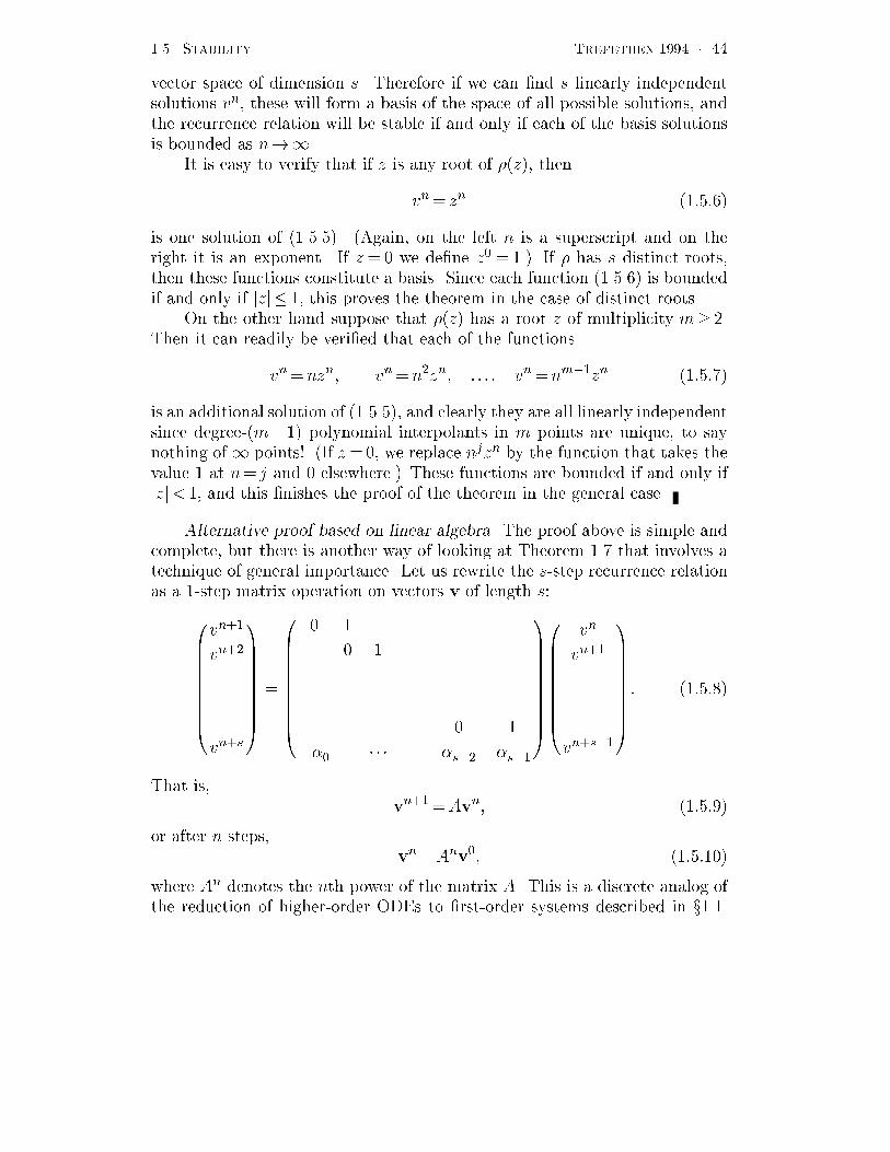
Alternative proof based on linear algebra� The proof above is simple andcomplete� but there is another way of looking at Theorem ��� that involves atechnique of general importance� Let us rewrite the s�step recurrence relationas a ��step matrix operation on vectors v of length s�
�BBBBBBBBB�
vn��
vn��
���
vn�s
CCCCCCCCCA�
�BBBBBBBBBB�
� �
� �
� � � � � �
� �
�� � � � ��s�� ��s��
CCCCCCCCCCA
�BBBBBBBBB�
vn
vn��
���
vn�s��
CCCCCCCCCA� �����
That is�vn���Avn� ������
or after n steps�vn�Anv� �������
where An denotes the nth power of the matrix A� This is a discrete analog ofthe reduction of higher�order ODEs to �rst�order systems described in x����
���� STABILITY TREFETHEN ���� � ��
The scalar sequence fvng will be bounded as n if and only if the vectorsequence fvng is bounded� and fvng will in turn be bounded if and only if theelements of An are bounded� Thus we have reduced stability to a problem ofgrowth or boundedness of the powers of a matrix�
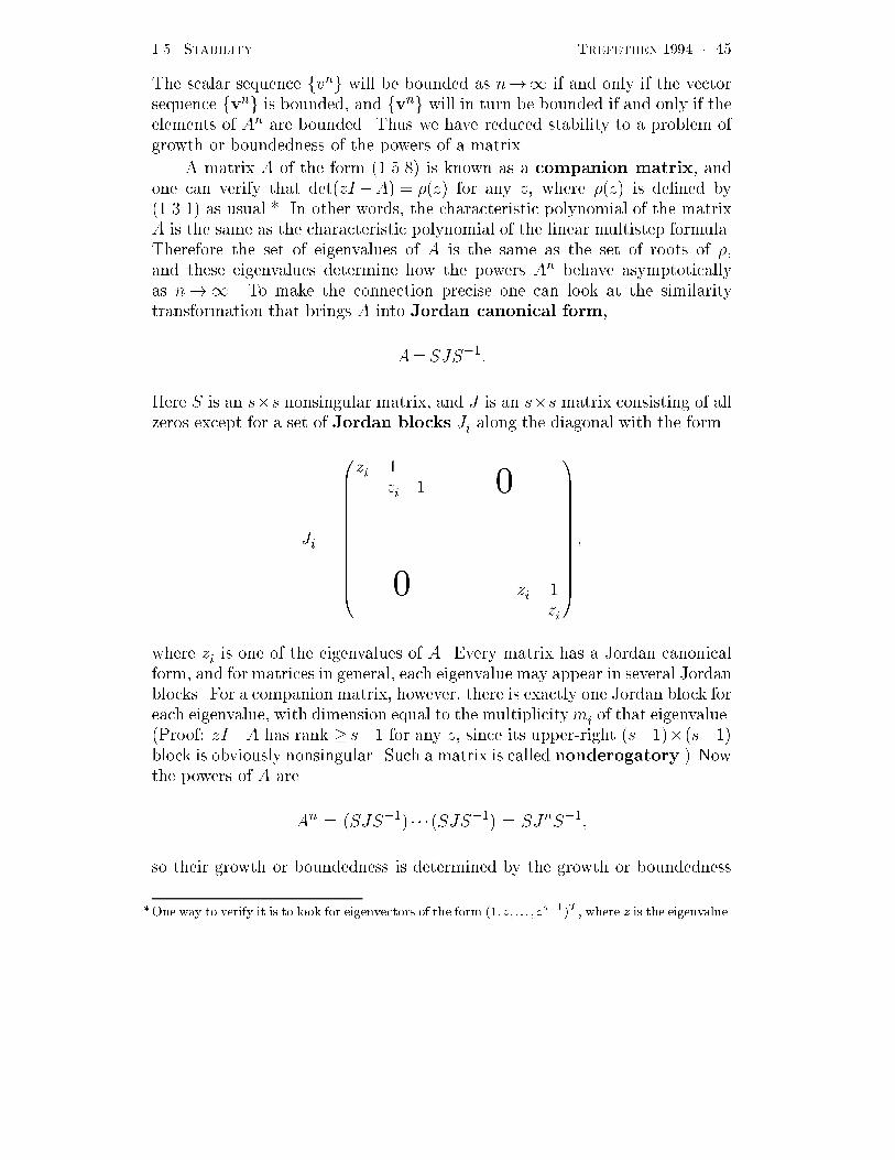
A matrix A of the form ����� is known as a companion matrix� andone can verify that det zI �A� � z� for any z� where z� is de�ned by ������ as usual�� In other words� the characteristic polynomial of the matrixA is the same as the characteristic polynomial of the linear multistep formula�Therefore the set of eigenvalues of A is the same as the set of roots of �and these eigenvalues determine how the powers An behave asymptoticallyas n � To make the connection precise one can look at the similaritytransformation that brings A into Jordan canonical form�
A�SJS���
Here S is an s�s nonsingular matrix� and J is an s�s matrix consisting of allzeros except for a set of Jordan blocks Ji along the diagonal with the form
Ji �
�BBBBBBBBBBBB�
zi �zi � �
� � � � � �
� zi �zi
CCCCCCCCCCCCA�
where zi is one of the eigenvalues of A� Every matrix has a Jordan canonicalform� and for matrices in general� each eigenvalue may appear in several Jordanblocks� For a companion matrix� however� there is exactly one Jordan block foreach eigenvalue� with dimension equal to the multiplicitymi of that eigenvalue� Proof� zI�A has rank � s�� for any z� since its upper�right s���� s���block is obviously nonsingular� Such a matrix is called nonderogatory�� Nowthe powers of A are
An � SJS��� � � � SJS��� � SJnS���
so their growth or boundedness is determined by the growth or boundedness
�One way to verify it is to look for eigenvectors of the form ��� z� � � � � zs���T where z is the eigenvalue�

���� STABILITY TREFETHEN ���� � �
of the powers Jn� which can be written down explicitly�
Jni �
�BBBBBBBBBBBBBBBBB�
zni�n�
�zn��i � � �
�n
mi��
�zn���mii
zni�n�
�zn��i
� � � � � ����
zni�n�
�zn��i
�zni
CCCCCCCCCCCCCCCCCA
�
If jzij� �� these elements approach � as n � If jzij� �� they approach �If jzij� �� they are bounded in the case of a ��� block� but unbounded ifmi� ��
The reader should study Theorem ��� and both of its proofs until he or sheis quite comfortable with them� These tricks for analyzing recurrence relationscome up so often that they are worth remembering�
EXAMPLE ������ Let us test the stability of various linear multistep formulas consideredup to this point� Any Adams�Bashforth or Adams�Moulton formula has z� � zs�zs���with roots f��� � � � �g� so these methods are stable� The Nystr$om and generalized Milne�Simpson formulas have z�� zs�zs��� with roots f������ � � � �g� so they are stable too�The scheme ������� that caused trouble in Example ����� has z�� z� �z��� with rootsf����g� so it is certainly unstable� As for the less dramatically unsuccessful formula �������it has z� � z���z �� z����� with a multiple root f���g� so it counts as unstable toosince it admits the growing solution vn�n� The higher�order extrapolation formula de�nedby z� � z���s� �z� � admits the additional solutions n��n�� � � � �ns��� making for aninstability more pronounced but still algebraic rather than exponential�
Note that by Theorem ���� any consistent linear multistep formula has aroot of z� at z � �� and if the formula is stable� then Theorem ��� ensuresthat this root is simple� It is called the principal root of � for it is theone that tracks the dierential equation� The additional consistency condition� �� � �� of Theorem ��� amounts to the condition that if z is perturbedaway from �� the principal root behaves correctly to leading order�
In x��� an analogy was mentioned between linear multistep formulas andrecursive digital �lters� In digital signal processing� one demands jzj� � forstability� why then does Theorem ��� contain the weaker condition jzj � �!The answer is that unlike the usual �lters� an ODE integrator must rememberthe past� even for values of t where f is zero� u is in general nonzero� If allroots z satis�ed jzj� �� the in�uence of the past would die away exponentially�

���� STABILITY TREFETHEN ���� � �
Theorem ��� leaves us in a remarkable situation� summarized in Figure������ By Theorem ���� consistency is the condition that z�� z� matcheslog z to at least second order at z � �� By Theorem ���� stability is the con�dition that all roots of z� lie in jzj � �� with simple roots only permittedon jzj� �� Thus the two crucial properties of linear multistep formulas havebeen reduced completely to algebraic questions concerning a rational function�The proofs of many results in the theory of linear multistep formulas� such asTheorems �� and ��� below� consist of arguments of pure complex analysis ofrational functions� having nothing super�cially to do with ordinary dierentialequations�
STABILITY zeros of z� in unit disk� simple if on unit circle
ORDER OF ACCURACY p�
z�
z�� logz�# z���p���
CONSISTENCY� p� �
Figure ������ Stability� consistency� and order of accuracy as alge�braic conditions on the rational function z�� z��
The following theorem summarizes the stability of the standard familiesof linear multistep formula that we have discussed�
STABILITY OF STANDARD LINEAR MULTISTEP FORMULAS
Theorem ���� The s�step Adams�Bashforth� Adams�Moulton� Nystr�om�and generalized Milne�Simpson formulas are stable for all s� �� The s�stepbackwards di�erentiation formulas are stable for �� s� �� but unstable fors� ��
Proof� The results for the �rst four families of linear multistep formulasfollow easily from Theorem ���� as described in Example ������ The analy�sis of backwards dierentiation formulas is a more complicated matter� since

���� STABILITY TREFETHEN ���� � ��
the polynomials z� are no longer trivial� Instability for s � � was recog�nized numerically in the �����s Mitchell and Craggs� ������ but not provedmathematically until ���� Cryer� ������ An elegant short proof of instabilityfor s� �� was devised by Hairer and Wanner in ��� and can be found onpp� ��%��� of Hairer� N�rsett Wanner� �����
To close this section we shall present an important result that is known asthe �rst Dahlquist stability barrier� In x��� we mentioned that an s�steplinear multistep formula can have order �s� why not simply use that high�order formula and forget special classes like Adams and Nystr&om methods!Dahlquist�s famous theorem con�rms that the answer is an impassable barrierof stability�
FIRST DAHLQUIST STABILITY BARRIER
Theorem ���� The order of accuracy p of a stable s�step linear multistepformula satis�es
p�
�����s�� if s is even�
s�� if s is odd�
s if the formula is explicit�
�������
Proof� Various proofs of Theorem ��� have been published� beginning withthe original one by Dahlquist in ����� More recent proofs have been based onthe beautiful idea of �order stars� introduced by Wanner� Hairer� and N�rsett BIT� ����� The following argument is adapted from �A proof of the �rstDahlquist barrier by order stars�� by A� Iserles and S� P� N�rsett� BIT� ����Though fundamentally correct� it is somewhat casual about geometric details�for a more detailed treatment see that paper or the book Order Stars by thesame authors�
Let z� and z� be the characteristic polynomials corresponding to astable s�step linear multistep formula of order of accuracy p� The key idea isto look at level lines of the function we have been dealing with since �������
� z� � z�
z�� logz� �������
This function is analytic throughout the complex plane except near zeros of z�� provided one introduces a branch cut going to the point z � �� Alter�
natively� one can work with e��z� and eliminate the need for a branch cut��In particular� � z� is analytic at z � �� If �� � �� z� and z� have a
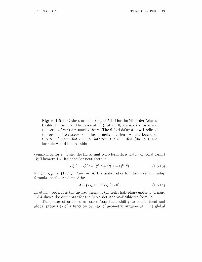
���� STABILITY TREFETHEN ���� � ��
Figure ����� Order star de�ned by ������� for the �th�order Adams�Bashforth formula� The zeros of z� at z��� are marked by o andthe zeros of z� are marked by �� The ��fold daisy at z�� re�ectsthe order of accuracy � of this formula� If there were a bounded�shaded ��nger� that did not intersect the unit disk dashed�� theformula would be unstable�
common factor z�� and the linear multistep formula is not in simplest form��By Theorem ���� its behavior near there is
� z� � C z���p���O z���p��� �������
for C �Cp��� �� � �� Now let A� the order star for the linear multistepformula� be the set de�ned by
A� fz � C � Re� z�� �g� �������
In other words� it is the inverse image of the right half�plane under �� Figure����� shows the order star for the �th�order Adams�Bashforth formula�
The power of order stars comes from their ability to couple local andglobal properties of a function by way of geometric arguments� The global

���� STABILITY TREFETHEN ���� � ��
property that concerns us is stability� the zeros of z� must lie in the unitdisk� The local property that concerns us is order of accuracy� from �������it follows that near z � �� A must look like a daisy with p�� evenly spacedpetals�or ��ngers�� as they are sometimes called� In Figure ����� the numberof �ngers is ��
Since the linear multistep formula is stable� all the zeros of z� must liein A or possibly on its boundary in the case of a zero with jzj � ��� Thisfollows from ������� and ������� since the zeros have to satisfy jzj � �� henceRe logz� �� �At this point some reasoning by the argument principle of com�plex analysis is needed� which will be �lled in later�� The conclusion is this�any bounded �nger of A i�e�� not extending to � must contain one of thezeros of z�� Consequence� for stability� every bounded �nger has to intersect
the unit disk�To �nish the argument� let us now assume that the linear multistep for�
mula is explicit� similar arguments apply in the implicit case Exercise �������Our goal is then to prove p� s� To do this we shall count zeros of Re� z� onthe unit circle jzj��� Let M be this number of zeros� counted with multiplic�ity� obviously M must be even� How big can M be! Note �rst that
�Re� z� � z�
z��
z�
z��
z� z�� z� z�
z� z�
on the unit circle jzj� �� since Relogz � � there� Since the linear multistepformula is explicit� z� has degree � s��� so the numerator is a polynomialof degree � �s��� which implies that M � being even� satis�es
M � �s��� �������
Now� how many zeros are implied by order of accuracy p! First� there is a zeroof multiplicity p�� at z��� In addition� there is a zero wherever the boundaryof A crosses the unit circle�in Figure ������ four such zeros altogether� Tocount these� we note that p����� �ngers of A begin at z � � outside theunit circle� One of these may be unbounded and go to in�nity� but the other p����� must intersect the unit disk and cross the unit circle on the way� Twoof those may cross the unit circle just once one each in the upper and lowerhalf�planes�� but all the remaining p����� �ngers are trapped inside those�ngers and must cross the unit circle twice� All told� we count
M � p������ p����� � �p��� �������
Combining ������� and ������� gives p� s� as required�Similar arguments apply if the linear multistep formula is implicit�

���� STABILITY TREFETHEN ���� � ��
The restrictions of Theorem ��� are tight" In eect� they show� half of theavailable parameters in a linear multistep formula are wasted�
Theorems ���� ��� and ��� imply that the Adams�Bashforth and Nystr&omformulas are all optimal in the sense that they attain the bound p� s for sta�ble explicit formulas� and the Adams�Moulton and generalized Milne�Simpsonformulas of odd step number s are also optimal� with p � s��� Simpson�srule� with p� s��� is an example of an optimal implicit formula with evenstep number� It can be shown that for any optimal implicit formula with evenstep number s� the roots of z� all lie on the unit circle jzj�� Henrici� �����p� ����� Thus the stability of these formulas is always of a borderline kind�
EXERCISES
� ����� Backwards di�erentiation formulas� Show that the following backwards di�erentia�tion formulas from Table ����� are stable� �a� s��� �b� s���
� ����� Prove�
�a� Any consistent ��step linear multistep formula is stable�
�b� Any consistent linear multistep formula with z���z� is unstable�
� ����� Consider the s�step explicit linear multistep formula of optimal order of accuracy ofthe form vns� vn k
Ps��j � jf
nj �
�a� For which s is it stable�
�b� Derive the coe�cients for the case s���
�c� Likewise for s���
� ���� Pad�e approximation� The type ���� Pad�e approximant to log z at z�� is de�nedas the unique rational function z���z� of type ���� i�e�� with numerator of degree �and denominator of degree �� that satis�es
z�
�z�� log z Oz������� as z� �� �����!�
By Theorem ���� taking �� �� s gives the maximally accurate implicit s�step formula� withorder of accuracy at least p��s� and taking �� s� � � s�� gives the maximally accurateexplicit s�step formula� with order of accuracy at least p��s���
Without performing any calculations� but appealing only to the uniqueness of Pad%e approx�imants and to theorems stated in this text� determine whether each of the following Pad%eschemes is stable or unstable� and what it is called if we have given a name for it� In eachcase� state exactly what theorems you have used�
�a� s��� explicit� �b� s��� implicit�
�c� s��� explicit� �d� s��� implicit�
�e� s��� explicit� �f� s��� implicit�
�g� If you have access to a symbolic calculator such as Macsyma� Maple� or Mathematica�use it to calculate the coe�cients of the linear multistep formulas �a���f�� and con�rmthat the names you have identi�ed above are correct�

���� STABILITY TREFETHEN ���� � ��
� ���� Linear combinations of linear multistep formulas� In Example ����� we showed thatthe trapezoid formula has error constant � �
�� and the midpoint formula has error constant�� �
�a� Devise a linear combination of these two formulas that has order of accuracy higherthan �� What is the order of accuracy�
�b� Show that the formula of �a� is stable�
�c� In general� is a convex linear combination of two stable linear multistep formulas alwaysstable� A convex linear combination has the form a�formula� ��a��formula� with a ��� Prove it or give a counterexample�
������� ����� Order stars� Write a program to generate order star plots like that of Figure ������This may be reasonably easy in a higher�level language like Matlab� Plot order stars for thefollowing linear multistep formulas� among others�
�a� �th�order Adams�Bashforth�
�b� �th�order Adams�Moulton�
�c� �th�order backwards di�erentiation�
�d� the unstable formula ��������
� ����� The proof of Theorem ��� in the text covered only the case of an explicit linearmultistep formula� Show what modi�cations are necessary for the implicit case�
���� THE DAHLQUIST EQUIVALENCE THEOREM TREFETHEN ���� � ��
��� Convergence and the Dahlquist
equivalence theorem
Up to this point we have talked about accuracy� consistency� and stability� but we haveyet to establish that a linear multistep formula with these admirable properties will actuallywork� After one more de�nition we shall be able to remedy that� To set the stage� let usreturn to the footnote on p� ��� If a linear multistep formula has local accuracy Okp���how can it fail to have global accuracy Okp�� The answer has nothing to do with the factthat f may be nonlinear� for we have assumed that f is Lipschitz continuous� and that isenough to keep the behavior of small perturbations essentially linear� so long as they remainsmall�
The &aw in the Okp� argument is as follows� Even though a discretization error maybe small when it is �rst introduced� from that point on it may grow�often exponentially�The global error at step n consists of the superposition not simply of the local errors atall previous steps� but of what these local errors have become at step n� Consistency is thecondition that the local errors are small at the time that they are introduced� provided thatthe function being dealt with is smooth� The additional condition of stability is needed tomake sure that they do not become bigger as the calculation proceeds�
The purpose of this section is to describe the ideas related to the Dahlquist EquivalenceTheorem that have been built to describe these phenomena� The rigorous statement of theargument above appears in the proof of Theorem ���� below� If f is linear� the argumentbecomes simpler� see Exercise ������
To begin we must de�ne the notion of convergence� The standard de�nition requiresthe linear multistep formula to be applicable not just to a particular initial�value problem�but to an arbitrary initial�value problem with Lipschitz continuous data f � It must alsowork for any starting values v�� � � � �vs�� that satisfy the consistency condition�
kvn�u�k� o�� as k� � n s��� ������
Equivalent statements of the same condition would be
limkvn�u�k�� limvn � u�� or vn � u� o��
as k� for n s�� see Exercise ���b���
A linear multistep formula is convergent if� for all initial�value problems ������� satisfy�ing the conditions of Theorem ��� on an interval ��T �� and all starting values v�� � � � �vs��
satisfying �������� the solution vn satis�es
kvt��ut�k� o�� as k� ������
uniformly for all t� ��T ��
�The choice of the norm k � k doesn�t matter since all norms on a �nite�dimensional space areequivalent� For a scalar ODE the norm can be replaced by the absolute value�
���� THE DAHLQUIST EQUIVALENCE THEOREM TREFETHEN ���� � ��
�Uniformly� means that kvt��ut�k is bounded by a �xed function �k�� o�� as k� �independent of t�� To put it in words� a convergent linear multistep formula is one thatis guaranteed to get the right answer in the limit k� � for each t in a bounded interval��T ��assuming there are no rounding errors�
Some remarks on this de�nition are in order� First� ������ is a statement about thelimit k� for each �xed value of t� Since vt� is de�ned only on a discrete grid� this meansthat k is implicitly restricted to values t�n in this limit process� However� it is possible toloosen this restriction by requiring only tnk � t as k� �
Second� to be convergent a linear multistep formula must work for all well�posedinitial�value problems� not just one� This may seem an unnaturally strict requirement� butit is not� A formula that worked for only a restricted class of initial�value problems�forexample� those with su�ciently smooth coe�cients�would be a fragile object� sensitive toperturbations�
Third� vn refers to the exact solution of the linear multistep formula� rounding errorsare not accounted for in the de�nition of convergence� This is a reasonable simpli�cationbecause discretization errors and errors in the starting values are included� via ������� andthe stability phenomena that govern these various sources of error are nearly the same�Alternatively� the theory can be broadened to include rounding errors explicitly�
Finally� note that condition ������ is quite weak� requiring only o�� accuracy of start�ing values� or Ok� if the errors happen to follow an integral power of k� This is in contrastto the Ok�� accuracy required at subsequent time steps by the de�nition of consistency�The reason for this discrepancy is simple enough� starting errors are introduced only at stime steps� while subsequent errors are introduced "k��� times� Therefore one can getaway with one order lower accuracy in starting values than in the time integration� Forpartial di�erential equations we shall �nd that analogously� one can usually get away withone order lower accuracy in discretizing boundary conditions�
We come now to a remarkable result that might be called the fundamental theoremof linear multistep formulas� Like much of the material in this and the last section� it �rstappeared in a classic paper by Germund Dahlquist in ������
DAHLQUIST EQUIVALENCE THEOREM
Theorem ����� A linear multistep formula is convergent if and only if it is consistentand stable�
Before proving this theorem� let us pause for a moment to consider what it says� Itseems obvious that a linear multistep formula that admits unstable solutions is unlikely tobe useful� but it is not so obvious that instability is the only thing that can go wrong� Forexample� clearly the extrapolation formula ������ of Example ����� must be useless� since itignores ffng� but why should that have anything to do with instability� Yet Theorem ���asserts that any useless consistent formula must be unstable� And indeed� we have veri�edthis prediction for ������ in Example ������
�G� Dahlquist Convergence and stability in the numerical integration of ordinary di�erential equa�tions� Math Scand � ������ ������ There are important earlier references in this area toonotably an in�uential article by Richard von Mises in ��� who proved convergence of Adamsmethods� The classic reference in book form on this material is P� Henrici Discrete Variable Meth�ods in Ordinary Di�erential Equations Wiley ����� A modern classic is the two�volume series byHairer N rsett and Wanner�
���� THE DAHLQUIST EQUIVALENCE THEOREM TREFETHEN ���� � ��
An indication of the power of Theorem ��� is that here� as in all of the developments ofthis chapter� the initial�value problems under consideration may be linear or nonlinear� Forpartial di�erential equations we shall see that the best known analog of Theorem ����theLax Equivalence Theorem�requires linearity�
Proof� Theorem ��� is not mathematically deep� the art is in the de�nitions� To proveit we shall establish three implications�
�a� convergent stable��b� convergent consistent��c� consistent stable convergent�
In outline� �a� and �b� are proved by applying the linear multistep formula to particularinitial�value problems ������� and �c� is proved by verifying that so long as one has stability�local errors cannot add up too much�
�a� Convergent stable� If the linear multistep formula is convergent� then ������must hold in particular for the initial�value problem ut � � u� � � whose solution isut�� � Now suppose the formula is unstable� Then by the proof of Theorem ��!� it admitsa particular solution V n� zn with jzj� �� or V n�nzn with jzj��� In either case� supposethe starting values for the time integration are taken as
vn�pkV n� n s��� ������
where k is as always the time step� Then the computed solution for all n will be preciselypkV n� But whereas the factor
pk ensures that the starting values approach u� � as
k� � as required by ������� jpkV nj approaches � for any t�nk � � Thus ������ doesnot hold� and the formula is not convergent�
�b� Convergent consistent� To prove consistency� by Theorem ���� we must show��� and �������� For the �rst� consider the particular initial�value problem ut��u� � �� whose solution is ut�� �� and the particular initial values v� � � � � � vs�� � ��Since fu�t� � � the linear multistep formula reduces to ������� and convergence impliesthat the solutions to this recurrence relation for the given initial data satisfy v��� � ask� � Since vn does not depend on k� this is the same as saying vn� � as n�� for �xedk � � and by ������� this implies ��� �
To show ��� � ���� consider the particular initial�value problem ut � �� u� � �with exact solution ut�� t � Since fu�t� � �� the linear multistep formula ������ reducesto Z�vn� k���� Now since Z� is a polynomial of degree s with ��� � it has a �niteTaylor expansion
Z� � ���Z��� �
�����Z���� � � � �
s��s���Z���s�
Let us apply Z� to the particular function V n� kn�������� tn�������� Since V n is
linear in n� all but the �rst term in the series are � and we get Z�V n � ���Z���V n�which reduces to k���� In other words� V n is a solution to the linear multistep formula ifthe prescribed initial values are vn � V n for n s��� Obviously this solution satis�escondition ������ for the given initial data u� � � For the linear multistep formula to beconvergent� it follows that V n must satisfy ������� and thus we must have ��� � ���� asclaimed�
�c� Consistent � stable convergent� �This part of the proof is not yet written� seethe references� such as pp� ��� ��� of Hairer� N'rsett� # Wanner ���!�� Following work of
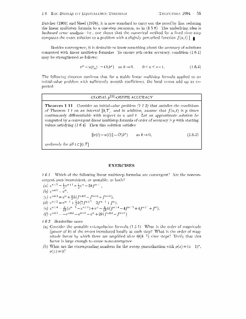
���� THE DAHLQUIST EQUIVALENCE THEOREM TREFETHEN ���� � �
Butcher ����� and Skeel ��!��� it is now standard to carry out the proof by �rst reducingthe linear multistep formula to a one�step recursion� as in ������� The underlying idea isbackward error analysis�i�e�� one shows that the numerical method for a �xed time stepcomputes the exact solution to a problem with a slightly perturbed function fu�t���
Besides convergence� it is desirable to know something about the accuracy of solutionscomputed with linear multistep formulas� To ensure pth�order accuracy� condition ������may be strengthened as follows�
kvn�utn�k�Okp� as k� � n s��� ������
The following theorem con�rms that for a stable linear multistep formula applied to aninitial�value problem with su�ciently smooth coe�cients� the local errors add up as ex�pected�
GLOBAL pTH�ORDER ACCURACY
Theorem ����� Consider an initial�value problem ������� that satis�es the conditionsof Theorem ��� on an interval ��T �� and in addition� assume that fu�t� is p timescontinuously di�erentiable with respect to u and t� Let an approximate solution becomputed by a convergent linear multistep formula of order of accuracy � p with startingvalues satisfying ������� Then this solution satis�es
kvt��ut�k�Okp� as k� � ������
uniformly for all t� ��T ��
EXERCISES
� ������ Which of the following linear multistep formulas are convergent� Are the noncon�
vergent ones inconsistent� or unstable� or both�
�a� vn�� ��v
n� ��v
n �kfn��
�b� vn�� vn�
�c� vn�� vn ��kf
n� fn� fn���
�d� vn�� vn� ��k!f
n���fn� fn��
�e� vn�� �� v
n��vn�� vn ��kf
n� �fn� �fn� fn��
�f� vn���vn� vn� vn �kfn� fn���
� ������ Borderline cases�
�a� Consider the unstable extrapolation formula ������� What is the order of magnitudepower of k� of the errors introduced locally at each step� What is the order of mag�nitude factor by which these are ampli�ed after "k��� time steps� Verify that thisfactor is large enough to cause nonconvergence�
�b� What are the corresponding numbers for the s�step generalization with z�� z���s��z�� �
���� THE DAHLQUIST EQUIVALENCE THEOREM TREFETHEN ���� � �
�c� On the other hand� devise another unstable linear multistep formula in which the localdiscretization errors are of a high enough order of accuracy relative to the unstableampli�cation factors that they will not cause nonconvergence�
�d� Why does the example of �c� not contradict Theorem ���� Why is it appropriate toconsider this example unstable�
� ������ Convergence for scalar linear initial�value problems� Prove as brie&y and elegantlyas you can that stability and consistency imply convergence� for the special case in which uis scalar and the function fu�t� is scalar and linear�

��!� STABILITY REGIONS TREFETHEN ���� � ��
��� Stability regions
The results of the last two sections concerned the behavior of linear multistep formulasin the limit k� � But for the important class of sti� ODEs� which involve widely varyingtime scales� it is impractical to take k small enough for those results to apply� Analysis ofbehavior for �nite k becomes indispensable� In Chapter � we shall see that consideration of�nite k is also essential for the analysis of discretizations of partial di�erential equations�
Sti�ness is a subtle idea� and our discussion of it will be deferred to the next section�Here� we shall simply consider the problem of �nite k analysis of linear multistep formulas�The key idea that emerges is the idea of a stability region�
EXAMPLE ������ Let us begin by looking again at the unstable third�order formula�������� In Example ����� we applied this formula to the initial�value problem ut � u�u� � � with time step k���� and observed the oscillatory instability shown in Figure�����b�� From one time step to the next� the solution grew by a factor about ������ andto explain this we looked at the recurrence relation
Z�vn � vn� �vn���vn � � ��!���
The zeros of z� are � and ��� corresponding to solutions vn�� and vn����n to ��!����and the second of these solutions explains the factor ����� at least approximately�
For this scalar� linear example� we can do much better by retaining the terms fnj inthe analysis� The function f is simply fu��u� and thus an exact rather than approximatemodel of the calculation is the recurrence relation
Z�vn�k�Z�fn � Z��k�Z��vn � � ��!���
that is�
Z� ���k�Z�� �k��vn � vn� ���k�vn��� �k�vn � �
Setting k���� gives the zeros
z�� �������� z������������
And now we have a virtually exact explanation of the ratio ������ of Exercise ������accurate� as it happens� to about � digits of accuracy see Exercise ��!����
For an arbitrary ODE� f is not just a multiple of u� and �nite k analysisis not so simple as in the example just considered� We want to take the terms�jf
n�j into consideration� but we certainly don�t want to carry out a separateanalysis for each function f � Instead� let us assume that f u�t�� au for someconstant a� C � In other words� we consider the linear model equation
ut� au� ������

��!� STABILITY REGIONS TREFETHEN ���� � ��
In the next section we shall see that a nonlinear system of ODEs can be reducedto a set of problems of the form ������ by linearization� freezing of coe�cients�and diagonalization�
If a linear multistep formula ������� is applied to the model equation ������� it reduces to the recurrence relation
sXj�
�jvn�j�'k
sXj�
�jvn�j � ��
or equivalently h Z��'k Z�
ivn � �� ������
where we have de�ned'k� ak� ������
Now let �!k z� be the stability polynomial
�!k z� � z��'k z� �sX
j�
�j�'k�j�z
j � ������
whose coe�cients depend on the parameter 'k� Then the solutions to ������are related to the zeros of �!k exactly as the solutions to ������ were relatedto the zeros of z�� In analogy to the developments of x���� we de�ne�
A linear multistep formula is absolutely stable� for a particular value'k � ak if all solutions fvng of the recurrence relation ������ are boundedas n �
Just as in Theorem ���� it is easy to characterize those linear multistep formulasthat are absolutely stable�
ROOT CONDITION FOR ABSOLUTE STABILITY
Theorem ����� A linear multistep formula is absolutely stable for a par�ticular value 'k� ak if and only if all the zeros of �!k z� satisfy jzj � �� andany zero with jzj�� is simple�
What is dierent here from what we did in x��� is that everything dependson 'k� For some 'k a linear multistep formula will be absolutely stable� and forothers it will be absolutely unstable� Here now is the key de�nition�
�Other terms are weakly stable� and time�stable��

��!� STABILITY REGIONS TREFETHEN ���� � �
The stability region S of a linear multistep formula is the set of all 'k � C
for which the formula is absolutely stable�
Note that according to this de�nition� a linear multistep formula is stable ifand only if the point � belongs to its stability region�
Let us now derive the four most familiar examples of stability regions�illustrated in Figure ������
EXAMPLE ������ For the Euler formula ������� ��!��� becomes
��kz� � z����(k � z�� (k�� ��!�!�
with zero � (k� Therefore S is the set of (k � C with j� (kj �� that is� the disk j(k����j ��Figure ��!��a plots this region�
EXAMPLE ������ For the backward Euler formula ������� the stability polynomial is
��kz� � z����(kz � ��(k�z��� ��!���
with zero ��(k���� S is the set of (k � C with j��(kj�� �� that is� the exterior of the diskj(k��j � �� See Figure ��!��b�
EXAMPLE ������ For the trapezoid formula ������� we have
��kz� � z���� ��(kz �� � �� �
�(k�z�� �
�(k� ��!���
with zero � ��(k���� �
�(k�� � (k����(k�� S is the set of points in C that are no farther
from �� than from ��i�e�� Rez � the left half�plane� See Figure ��!��c�
EXAMPLE ������ The midpoint formula ������ has
��kz� � z���(kz��� ��!���
which has two zeros z satisfying
z� �
z��(k� ��!����
Obviously there is always one zero with jz�j � and another with jz�j � �� so for absolutestability� we must have jz�j� jz�j� � �both zeros on the unit circle� which will occur ifand only if (k lies in the closed complex interval ��i� i �� The two extreme values (k��i givedouble zeros z� � z� ��i� so we conclude that S is the open complex interval �i� i�� asshown in Figure ��!��d�
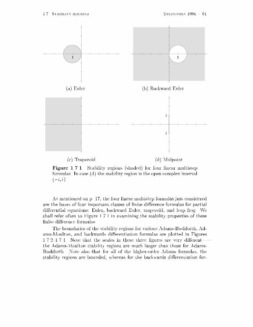
��!� STABILITY REGIONS TREFETHEN ���� � �
�� �
a� Euler b� Backward Euler
i
�i
c� Trapezoid d� Midpoint
Figure ������ Stability regions shaded� for four linear multistepformulas� In case d� the stability region is the open complex interval �i� i��
As mentioned on p� ��� the four linear multistep formulas just consideredare the bases of four important classes of �nite dierence formulas for partialdierential equations� Euler� backward Euler� trapezoid� and leap frog� Weshall refer often to Figure ����� in examining the stability properties of these�nite dierence formulas�
The boundaries of the stability regions for various Adams�Bashforth� Ad�ams�Moulton� and backwards dierentiation formulas are plotted in Figures�����%������ Note that the scales in these three �gures are very dierent�the Adams�Moulton stability regions are much larger than those for Adams�Bashforth� Note also that for all of the higher�order Adams formulas� thestability regions are bounded� whereas for the backwards dierentiation for�

��!� STABILITY REGIONS TREFETHEN ���� � �
mulas they are unbounded� As will be explained in the next section� this iswhy backwards dierentiation formulas are important�
How does one compute stability regions like these! One approach wouldbe to calculate the zeros of �!k for a large number of values of
'k� C and drawa contour plot� but there is a simpler and more accurate method� By �������if z is a zero of �!k z� for some
'k and z� ��� then
'k� z�
z� �������
cf� ��������� To determine the boundary of the stability region� �rst calculatethe curve of values 'k corresponding to z� ei with � � ������� This root locuscurve has the property that at each point 'k on the curve� one zero of �!k justtouches the unit circle� It follows that the boundary of S is a subset of the rootlocus curve�only a subset� in general� because the other zeros of �!k might lieeither in the disk or outside� By the principle of the argument of complexanalysis� one can determine which components are which by checking just onevalue 'k in each loop enclosed by the root locus curve� See Exercise ������
EXERCISES
� ������ Prove that for the unstable linear multistep formula �������� the stability region Sis the empty set�
� ������ Find exact formulas for the boundaries of S for �a� the second�order Adams�Bashforthformula� �b� the third�order backwards di�erentiation formula�
������� ������ Write a computer program to plot root locus curves� In a high�level language likeMatlab� it is most convenient to de�ne a variable r���z��� where z is a vector of � orso points on the unit circle� and then work directly with formulas such as ������� ��������������� rather than with the coe�cients �j and j �
�a� Reproduce Figure ��!��� and then generate the root locus curve for p��� What is S �Be careful��
�b� Reproduce Figure ��!��� and then generate the root locus curve for p�!� What is S �
�c� Plot the root locus curve for �������� Label each component by the number of zeros of��k outside the unit disk� and explain how this pictures relates to Exercise ��!���
� ����� What is the maximum time step k for which the third�order Adams�Bashforthformula is absolutely stable when applied to �i� ut��u� �ii� ut� iu�
�a� First� estimate the time step limits with the aid of Figure ��!�� and a ruler�
�b� Now derive the exact answers� For �ii� this is hard� but it can be done�
� ����� Explain the remark about ��digit accuracy at the end of Example ��!��� Approxi�mately where does the �gure of � digits come from�
� ������ True or False� the stability region for any linear multistep formula is a closed subsetof the complex plane�

��!� STABILITY REGIONS TREFETHEN ���� � �
i
�i
�����
p��
�
�
Figure ������ Boundaries of stability regions for Adams�Bashforthformulas of orders �%��
�� ��
�i
��i
p��
�
�
�
Figure ������ Boundaries of stability regions for Adams�Moultonformulas of orders �%�� Orders � and � were displayed already inFigure ����� b�c��� Note that the scale is very dierent from that ofthe previous �gure�
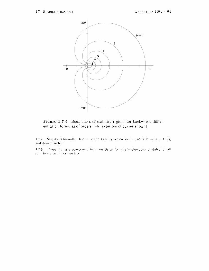
��!� STABILITY REGIONS TREFETHEN ���� � �
p��
�
�
��
�
���
��i
�i
Figure ����� Boundaries of stability regions for backwards dier�entiation formulas of orders �%� exteriors of curves shown��
� ������ Simpson�s formula� Determine the stability region for Simpson�s formula �����!��and draw a sketch�
� ������ Prove that any convergent linear multistep formula is absolutely unstable for allsu�ciently small positive (k � �
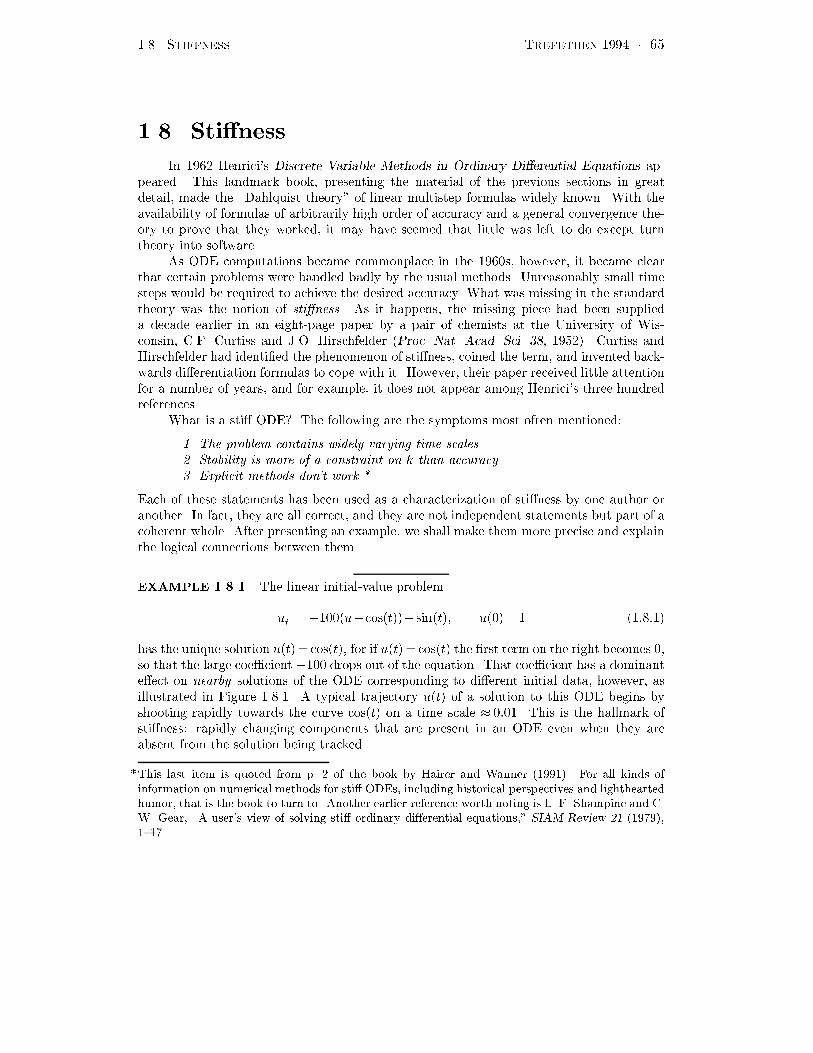
���� STIFFNESS TREFETHEN ���� � �
���� Sti�ness
In ���� Henrici�s Discrete Variable Methods in Ordinary Di�erential Equations ap�peared� This landmark book� presenting the material of the previous sections in greatdetail� made the �Dahlquist theory� of linear multistep formulas widely known� With theavailability of formulas of arbitrarily high order of accuracy and a general convergence the�ory to prove that they worked� it may have seemed that little was left to do except turntheory into software�
As ODE computations became commonplace in the ���s� however� it became clearthat certain problems were handled badly by the usual methods� Unreasonably small timesteps would be required to achieve the desired accuracy� What was missing in the standardtheory was the notion of sti�ness� As it happens� the missing piece had been supplieda decade earlier in an eight�page paper by a pair of chemists at the University of Wis�consin� C�F� Curtiss and J�O� Hirschfelder Proc� Nat� Acad� Sci� ��� ������ Curtiss andHirschfelder had identi�ed the phenomenon of sti�ness� coined the term� and invented back�wards di�erentiation formulas to cope with it� However� their paper received little attentionfor a number of years� and for example� it does not appear among Henrici�s three hundredreferences�
What is a sti� ODE� The following are the symptoms most often mentioned�
�� The problem contains widely varying time scales�
�� Stability is more of a constraint on k than accuracy�
�� Explicit methods don�t work�
Each of these statements has been used as a characterization of sti�ness by one author oranother� In fact� they are all correct� and they are not independent statements but part of acoherent whole� After presenting an example� we shall make them more precise and explainthe logical connections between them�
EXAMPLE �� ��� The linear initial�value problem
ut � ��u�cost���sint�� u�� � ������
has the unique solution ut�� cost�� for if ut�� cost� the �rst term on the right becomes �so that the large coe�cient �� drops out of the equation� That coe�cient has a dominante�ect on nearby solutions of the ODE corresponding to di�erent initial data� however� asillustrated in Figure ������ A typical trajectory ut� of a solution to this ODE begins byshooting rapidly towards the curve cost� on a time scale � ��� This is the hallmark ofsti�ness� rapidly changing components that are present in an ODE even when they areabsent from the solution being tracked�
�This last item is quoted from p� � of the book by Hairer and Wanner ������� For all kinds ofinformation on numerical methods for sti� ODEs including historical perspectives and lightheartedhumor that is the book to turn to� Another earlier reference worth noting is L� F� Shampine and C�W� Gear A user�s view of solving sti� ordinary di�erential equations� SIAM Review �� �����������

���� STIFFNESS TREFETHEN ���� �
t
Figure �� ��� ut�� cost� and nearby solutions of the initial�value problem �������
k AB� BD�
�� ���� ����
�� ���!��� �����
�� ������� �����
�� ���!!���� ������
�� ������� �������
�� ������� ����������
������
������� ������� � cos��
Table �� ��� Computed values v�� for the same problem�
** *** * ** * * * * ** * * * * * * * * * * * * * * * * * * * * * * * * * * * * * * * *
ooooo
ooo
oo
oo
ooo
oo
oo
o o o oo
o
o
o
o
o o o o o o o o o o o o o o o o o o
����
�
���
��� ��� ���
AB�
BD�
k
Figure �� ��� Computed errors jv���cos��j as a function of step size k for thesame problem log�log scale��
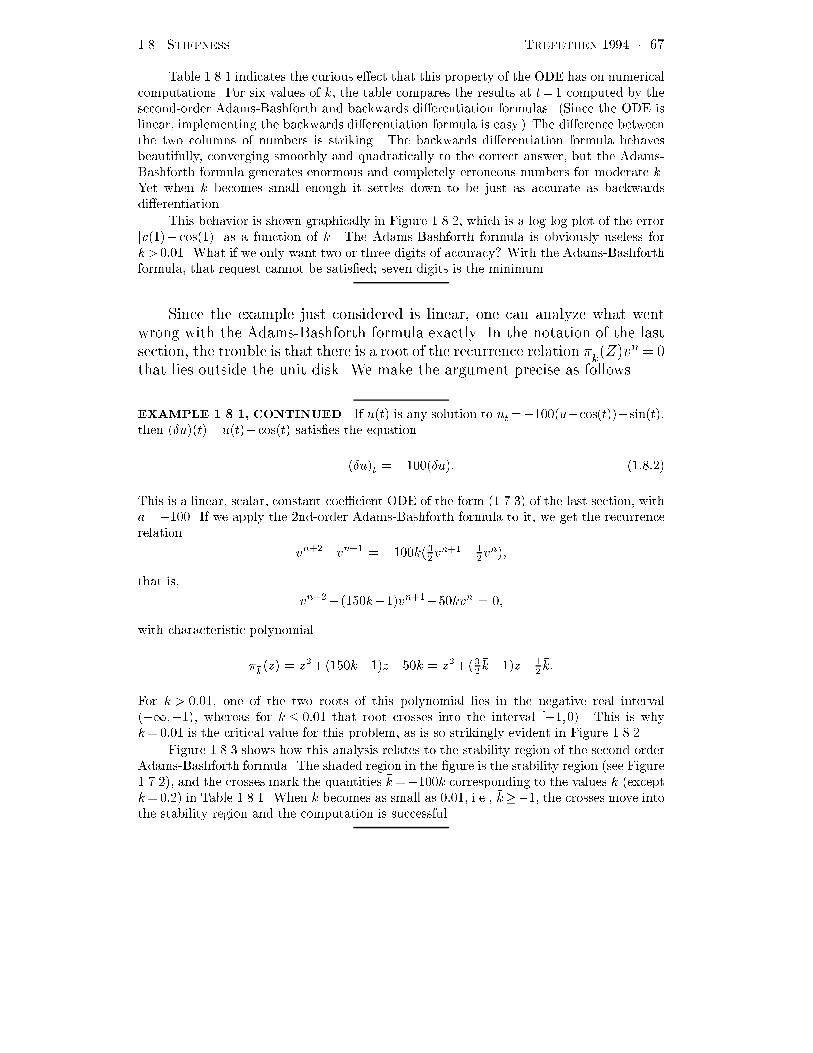
���� STIFFNESS TREFETHEN ���� �
Table ����� indicates the curious e�ect that this property of the ODE has on numericalcomputations� For six values of k� the table compares the results at t�� computed by thesecond�order Adams�Bashforth and backwards di�erentiation formulas� Since the ODE islinear� implementing the backwards di�erentiation formula is easy�� The di�erence betweenthe two columns of numbers is striking� The backwards di�erentiation formula behavesbeautifully� converging smoothly and quadratically to the correct answer� but the Adams�Bashforth formula generates enormous and completely erroneous numbers for moderate k�Yet when k becomes small enough it settles down to be just as accurate as backwardsdi�erentiation�
This behavior is shown graphically in Figure ������ which is a log�log plot of the errorjv��� cos��j as a function of k� The Adams�Bashforth formula is obviously useless fork � ��� What if we only want two or three digits of accuracy� With the Adams�Bashforthformula� that request cannot be satis�ed� seven digits is the minimum�
Since the example just considered is linear� one can analyze what wentwrong with the Adams�Bashforth formula exactly� In the notation of the lastsection� the trouble is that there is a root of the recurrence relation �!k Z�v
n��that lies outside the unit disk� We make the argument precise as follows�
EXAMPLE �� ��� CONTINUED� If ut� is any solution to ut���u�cost���sint��then �u�t��ut��cost� satis�es the equation
�u�t � ���u�� ������
This is a linear� scalar� constant�coe�cient ODE of the form ��!��� of the last section� witha���� If we apply the �nd�order Adams�Bashforth formula to it� we get the recurrencerelation
vn��vn� � ��k ��vn�� ��v
n��
that is�
vn� ��k���vn���kvn � �
with characteristic polynomial
��kz� � z� ��k���z��k � z� ��(k���z� �
�(k�
For k � ��� one of the two roots of this polynomial lies in the negative real interval������� whereas for k �� that root crosses into the interval ������ This is whyk��� is the critical value for this problem� as is so strikingly evident in Figure ������
Figure ����� shows how this analysis relates to the stability region of the second�orderAdams�Bashforth formula� The shaded region in the �gure is the stability region see Figure��!���� and the crosses mark the quantities (k���k corresponding to the values k exceptk���� in Table ������ When k becomes as small as ��� i�e�� (k���� the crosses move intothe stability region and the computation is successful�

���� STIFFNESS TREFETHEN ���� � �
x x x x x!k��� !k��� !k���k��� k��� k���
!k���
!k�� ��
Figure ������ The stability region for the �nd�order Adams�Bash�forth formula� with crosses marking the values 'k�����k from Table�����
With this example in mind� let us turn to a more careful discussion ofstatements �%� on p� ��� The following summary describes what it means tosay that the ODE ut � f u�t� is sti with respect to the solution u� t� fortimes t� t��
�� Widely varying time scales� Stiness arises when the time scale thatcharacterizes the evolution of u� t� for t� t� is much slower than the timescale that characterizes the evolution of small perturbations �u� t� on thatsolution for t� t��
�� Stability is more of a constraint than accuracy� If widely varying timescales in this sense are present� and if the discrete ODE formula has a boundedstability region� then there is a mismatch between the relatively large timesteps that are adequate to resolve u� t� and the relatively small time stepsthat are necessary to prevent unstable growth of small perturbations �u� t��A successful computation will necessitate the use of these small time steps�
�� Explicit methods don�t work� In particular� since explicit methodsalways have bounded stability regions Exercise ������ the solution of stiODEs by explicit methods necessitates the use of small time steps� For betterresults one must usually turn to implicit formulas with unbounded stabilityregions�
If the real world supplied ODEs to be solved �at random�� then widelyvarying time scales might not be a common concern� In actuality� the appli�cations that the real world presents us with are often exceedingly sti� Oneexample is the �eld of chemical kinetics� Here the ordinary dierential equa�tions describe reactions of various chemical species to form other species� andthe stiness is a consequence of the fact that dierent reactions take placeon vastly dierent time scales� Time scale ratios of ��� or more are common�Two other �elds in which sti ODEs arise frequently are control theory� wherecontrolling forces tend to be turned on and o again suddenly� and circuit sim�ulation� since dierent circuit components tend to have widely diering natural

���� STIFFNESS TREFETHEN ���� � �
frequencies�� A fourth important class of sti ordinary dierential equationsare the systems of ODEs that arise after discretizing time�dependent partialdierential equations� particularly parabolic problems� with respect to theirspace variables�the �method of lines�� This example will be discussed atlength in Chapter ��
To be able to determine whether a particular problem is sti� we needtools for quantifying the notion of the �time scales� present in an ODE� Theway this is generally done is by reducing an arbitrary system of ODEs to acollection of scalar� linear model problems of the form ������� to which theidea of stability regions will be applicable� This is achieved by the followingsequence of three steps� a sequence that has been familiar to mathematicalscientists for a century�
ut� f u�t� �����
� LINEARIZE
ut� J t�u �����
� FREEZE COEFFICIENTS
ut�Au �����
� DIAGONALIZE
fut��ug� ��( A�� �����
In ������ ( A� denotes the spectrum of A� i�e�� the set of eigenvalues�We begin with ������ a system ofN �rst�order ODEs� with u� t� denoting
the particular solution that we are interested in� If we make the substitution
u t�� u� t�� �u� t��
as in ������ then stability and stiness depend on the evolution of �u� t��The �rst step is to linearize the equation by assuming �u is small� If f is
dierentiable with respect to each component of u� then we have
f u�t� � f u�� t��J t� �u� t��o k�uk��
where J t� is the N �N Jacobian matrix of partial derivatives of f withrespect to u�
�J t��ij ��f �i�
�u�j� u� t�� t�� �� i� j�N�
�See A� Sangiovanni�Vincentelli and J� K� White Relaxation Techniques for the Solution of VLSICircuits Kluwer �����
���� STIFFNESS TREFETHEN ���� � �
This means that if �u is small� the ODE can be accurately approximated bya linear problem�
ut � f u�� t��J t� �u��
If we subtract the identity u�t � f u�� t� from this equation� we get
�u�t � J t� �u��
One can think of this result as approximate� if �u is small� or exact� if �u isin�nitesimal� Rewriting �u as a new variable u gives ������
The second step is to freeze coecients by setting
A� J t��
for the particular value t� of interest� The idea here is that stability andstiness are local phenomena� which may appear at some times t� and notothers� The result is the constant�coe�cient linear problem ������
Finally� assuming A is diagonalizable� we diagonalize it� In general� anysystem of N linear ordinary dierential equations with a constant� diagonal�izable coe�cient matrix A is exactly equivalent to N scalar equations ������with values a equal to the eigenvalues of A� To exhibit this equivalence� let Vbe anN�N matrix such that V ��AV is diagonal� The columns of V are eigen�vectors of A�� Then ut �Au can be rewritten as ut � V V ��AV �V ��u� i�e�� V ��u�t � V
��AV � V ��u�� a diagonal system of equations in the variablesV ��u� This diagonal system of ODEs can be interpreted as a representationof the original system ����� in the basis of eigenvectors of A de�ned by thecolumns of V � And thus� since a diagonal system of ODEs is the same as acollection of independent scalar ODEs� we end up with the N problems ������
Having reduced ����� to a collection of N scalar� linear� constant�coef��cient model problems� we now estimate stability and stiness as follows�
RULE OF THUMB� For a successful computation of u� t� for t� t�� k mustbe small enough that for each eigenvalue � of the Jacobian matrix J t���'k� k� lies inside the stability region S �or at least within a distance O k�of S��
This Rule of Thumb is not a theorem� exceptions can be found�� But if itis violated� some numerical mode will very likely blow up and obliterate thecorrect solution� Regarding the �gure O k�� see Exercise �����
�It is interesting to consider what keeps the Rule of Thumb from being a rigorous statement� Thevarious gaps in the argument can be associated with the three reductions ���������������� The step��������������� may fail if the actual discretization errors or rounding errors present in the problemare large enough that they cannot be considered in�nitesimal i�e� the behavior of u is nonlinear�

���� STIFFNESS TREFETHEN ���� � �
A sti problem is one for which satisfying the conditions of the Rule ofThumb is more of a headache than resolving the underlying solution u� t��
Here are some examples to illustrate the reduction ����� ������
EXAMPLE �� ��� If the equation in Example ����� had been
ut � ��sinu�cost���sint��
then linearization would have been called for� Setting �u�t��ut��cost� gives
�u�t���sin�u��
and if ut�� cost�� then �u�t� is small� and the linear model becomes ������ again�
EXAMPLE �� ��� For the initial�value problem
ut � ��u�t�sinu�cost���sint��
we end up with a model equation with a time�dependent coe�cient�
�u�t���cos�t��u��
These are scalar examples� However� the usual reason that an ODE haswidely varying time scales is that it is a system of dierential equations� If thesolution has N components� it is natural that some of them may evolve muchmore rapidly than others� Here are three examples�
EXAMPLE �� ��� Consider the ��� linear initial�value problem��u���
u���
At
�
����
��
A��u���
u���
A � t� �����
��u���
u���
A��
���
�
A � ����!�
Suppose we decide that an acceptable solution at t�� is any vector with jv������e�����j��and jv������e��j� � for some � � � If ����!� is solved by a pth order linear multistepformula with time step k� the u��� and u��� components decouple completely� so the results
The step ��������������� may fail if the density of time steps is not large compared with the timescale on which J�t� varies �D�J� Higham ������ The �nite size of the time steps also implies that ifan eigenvalue drifts outside the stability region for a short period the error growth it causes maybe small enough not to matter� Finally the step ��������������� may fail in the case where thematrix A is far from normal� i�e� its eigenvectors are far from orthogonal� In this case the matrixV is ill�conditioned and instabilities may arise even though the spectrum of A lies in the stabilityregion� it becomes necessary to consider the pseudospectra of A as well �D�J� Higham and L�N�T������� These e�ects of non�normality will be discussed in xx������� and turn out to be particularlyimportant in the numerical solution of time�dependent PDEs by spectral methods discussed inChapter ��
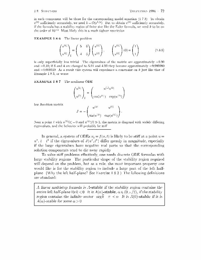
���� STIFFNESS TREFETHEN ���� � �
in each component will be those for the corresponding model equation ��!���� To obtainv��� su�ciently accurately� we need k�O���p�� But to obtain v��� su�ciently accurately�if the formula has a stability region of �nite size like the Euler formula� we need k to be onthe order of ���� Most likely this is a much tighter restriction�
EXAMPLE �� ��� The linear problem
��u���
u���
At
�
���� �
� ��
A��u���
u���
A �
��u���
u���
A��
���
�
A ������
is only super�cially less trivial� The eigenvalues of the matrix are approximately ����and ���� if � and � are changed to ��� and ���� they become approximately ��������and ���� As a result this system will experience a constraint on k just like that ofExample ������ or worse�
EXAMPLE �� ��� The nonlinear ODE��u���
u���
At
�
�� �u���u���
cosu�����expu����
A
has Jacobian matrix
J � ��� u��� u���
sinu���� expu����
A �
Near a point t with u���t�� and u���t� �� the matrix is diagonal with widely di�eringeigenvalues� and the behavior will probably be sti��
In general� a system of ODEs ut� f u�t� is likely to be sti at a point u�u�� t� t� if the eigenvalues of J u�� t�� dier greatly in magnitude� especiallyif the large eigenvalues have negative real parts so that the correspondingsolution components tend to die away rapidly�
To solve sti problems eectively� one needs discrete ODE formulas withlarge stability regions� The particular shape of the stability region requiredwill depend on the problem� but as a rule� the most important property onewould like is for the stability region to include a large part of the left half�plane� Why the left half�plane! See Exercise ������ The following de�nitionsare standard�
A linear multistep formula is A�stable if the stability region contains theentire left half�plane Re'k� �� It is A ���stable� �� ������� if the stabilityregion contains the in�nite sector jarg'k��j��� It is A ���stable if it isA ���stable for some �� ��

���� STIFFNESS TREFETHEN ���� � �
Roughly speaking� an A�stable formula will perform well on almost any stiproblem and of course also on non�sti problems� at some cost in extra workper time step�� An A ���stable formula will perform well on sti problemswhose component modes exhibit exponential decay negative real eigenvalues�but not oscillation imaginary eigenvalues�� Discretizations of parabolic andhyperbolic partial dierential equations� respectively� will provide good exam�ples of these two situations later in the book�
Figure ����� showed that both the backward Euler and trapezoid formulasare A�stable� This seems encouraging� perhaps to play it safe� we can simplyuse A�stable formulas all the time! But the following famous theorem showsthat that policy is too limiting�
SECOND DAHLQUIST STABILITY BARRIER
Theorem ����� The order of accuracy of an implicit A�stable linear mul�tistep formula satis�es p� �� An explicit linear multistep formula cannotbe A�stable�
Proof� Dahlquist� BIT ������ �Not yet written�
For serious computations� second�order accuracy is often not good enough�This is why backwards dierentiation formulas are so important� For all ofthe higher�order Adams formulas� the stability regions are bounded� but thebackwards dierentiation formulas are A ���stable for p � ��� Most of thesoftware in use today for sti ordinary dierential equations is based on theseformulas� though Runge�Kutta methods are also contenders see the next sec�tion�� Because of Theorem ��� the usable backwards dierentiation formulasare only those with p� �� In practice� some codes restrict attention to p� ��
Of course there are a dozen practical issues of computation for sti ODEsthat we have not touched upon here� For example� how does one solve thenonlinear equations at each time step! The answer is invariably some form ofNewton�s method� see the references�� The state of software for sti problemsis highly advanced� as is also true for non�sti problems� A non�sti solverapplied to a sti problem will typically get the right answer� but it will takeexcessively small time steps� Many such codes incorporate devices to detectthat stiness is present and alert the user to that fact� or in some cases� totrigger an automatic change to a sti solution method�
EXERCISES
� ������ Prove that the stability region of any explicit linear multistep formula is bounded�
�For p�������� the values of � involved are approximately ��� ��� ��� ���� See Figure ������
���� STIFFNESS TREFETHEN ���� � �
� ������ Suppose Figure ����� had been based on the error jv���cos��j instead of jv���cos��j� Qualitatively speaking� how would the plot have been di�erent�
� ������ What is special about the left half�plane that makes it appear in the de�nition ofA�stability� Avoid an answer full of wa)e� write two or three sentences that hit the nail onthe head�
� ����� The Rule of Thumb of p� ! mentions the distance Ok� from the stability region�Explain where this �gure comes from� perhaps with the aid of an example� Why is it Ok�rather than� say� Ok�� or Ok�����
� ����� Here is a second�order initial�value problem�
uttt�� costutt�� ut��� t� u�� �� ut�� �
�a� Rewrite it as a �rst�order initial�value problem of dimension ��
�b� Write down the precise formula used to obtain vn� at each step if this initial�valueproblem is solved by the second�order Adams�Bashforth formula�
�c� Write down the ��� Jacobian matrix J for the system �a��
� ������ An astronomer decides to use a non�sti� ODE solver to predict the motion of Jupiteraround the sun over a period of �� years� Saturn must certainly be included in thecalculation if high accuracy is desired� and Neptune and Uranus might as well be thrown infor good measure� Now what about Mars� Earth� Venus� and Mercury� Including these innerplanets will improve the accuracy slightly� but it will increase the cost of the computation�Estimate as accurately as you can the ratio by which it will increase the computation timeon a serial computer� Hint� your favorite almanac or encyclopedia may come in handy��
� ������ A linear multistep formula is A�stable� What can you conclude about the roots of�z��
� ������ Van der Pol oscillator� The equation �utt � �u ��u��ut� known as the Van der Polequation� represents a simple harmonic oscillator to which has been added a nonlinear termthat introduces positive damping for juj� � and negative damping for juj� �� Solutionsto this equation approach limit cycles of �nite amplitude� and if � is small� the oscillationis characterized by periods of slow change punctuated by short intervals during which ut�swings rapidly from positive to negative or back again�
�a� Reduce the Van der Pol equation to a system of �rst�order ODEs� and compute theJacobian matrix of this system�
�b� What can you say about the sti�ness of this problem�
� ������ Given �� �� suppose you solve an initial�value problem involving the linear equationut��Au ft�� where A is a constant ��� matrix with eigenvalues �� ������ and ���� andft� is a slowly�varying vector function of dimension �� You solve this equation by a linearmultistep program that is smart enough to vary the step size adaptively as it integrates� andyour goal is to compute the solution u�� accurate to within an absolute error on the orderof �� �� How many time steps order of magnitude functions of � and �� will be neededif the program uses �a� the second�order Adams�Moulton method� and �b� the third�orderAdams�Moulton method� Hint� be careful��
������� ������� A nonlinear sti� ODE� �To appear

���� RUNGE�KUTTA METHODS TREFETHEN ���� � �
���� Runge Kutta methods
Linear multistep formulas represent one extreme�one function evaluation per timestep�and Runge�Kutta methods represent the other� They are onestep� multistage meth�ods� in which fu�t� may be evaluated at any number of stages in the process of getting fromvn to vn�� but those stages are intermediate evaluations that are never used again� As aresult� Runge�Kutta methods are often more stable than linear multistep formulas� but atthe price of more work per time step� They tend to be easier to implement than linear multi�step formulas� since starting values are not required� but harder to analyze� These methodswere �rst developed a century ago by Runge ������ Heun ���� and Kutta �����
In this book we will not discuss Runge�Kutta methods in any detail� we merely list afew of them� below� and state two theorems without proof� This is not because they areless important than linear multistep methods� but merely to keep the scale of the bookmanageable� Fortunately� the fundamental concepts of stability� accuracy and convergenceare much the same for Runge�Kutta as for linear multistep formulas� The details are quitedi�erent� however� and quite fascinating� involving a remarkable blend of ideas of combina�torics and graph theory� For information� see the books by Butcher and by Hairer� N'rsett�and Wanner�
Runge�Kutta formulas tend to be �not very unique�� If we de�ne
s� numbers of stages� p� order of accuracy�
then for most values of s there are in�nitely many Runge�Kutta formulas with the maximalorder of accuracy p� Here are some of the best�known examples �which should properly bepresented in tableau form� but I haven�t gotten around to that��
�Modi�ed Euler� or �improved polygon� formula s� p���
a �� kfvn� tn��
b �� kfvn a��� tn k����
vn� �� vn b�
������
�Improved Euler� or �Heun� formula s� p���
a �� kfvn� tn��
b �� kfvn a� tn k��
vn� �� vn �� a b��
������
�Heun�s third�order formula� s� p���
a �� kfvn� tn��
b �� kfvn a��� tn k����
c �� kfvn �b��� tn �k����
vn� �� vn �� a �c��
������
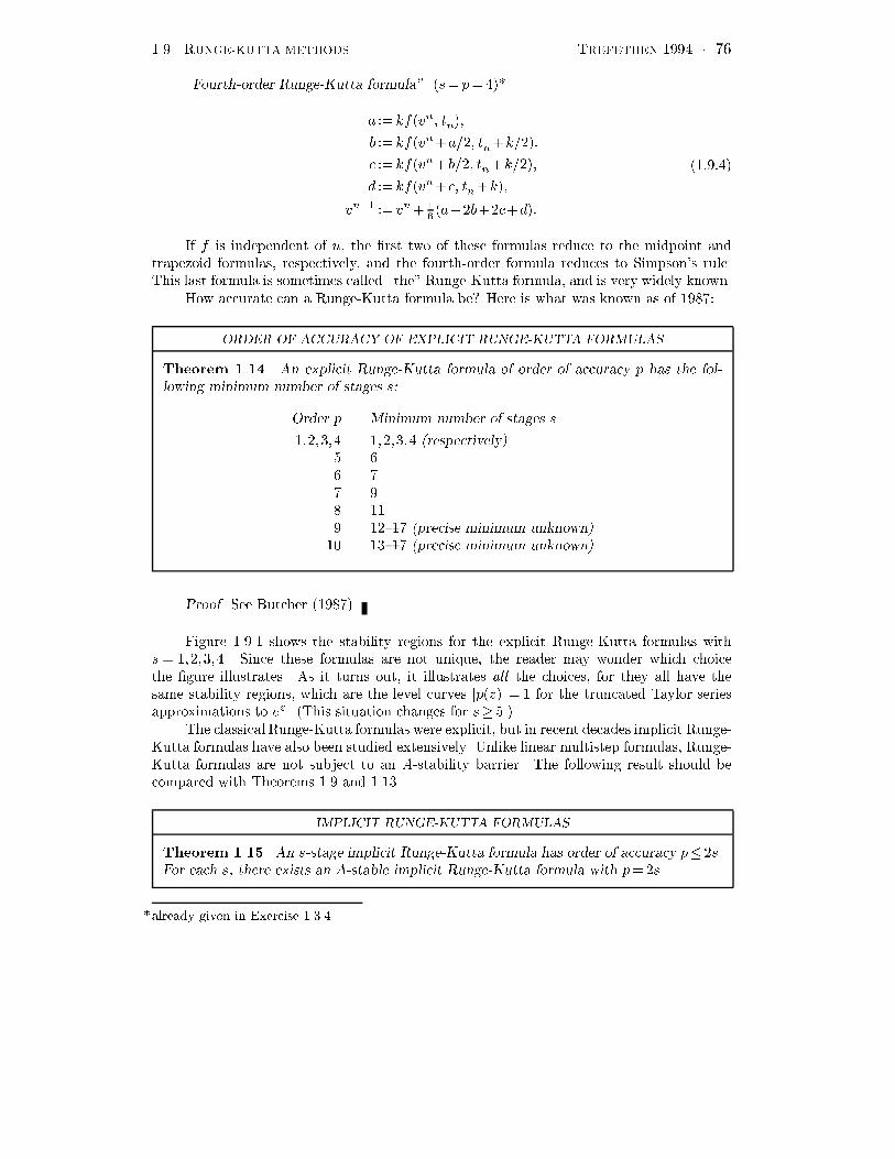
���� RUNGE�KUTTA METHODS TREFETHEN ���� �
�Fourth�order Runge�Kutta formula� s� p����
a �� kfvn� tn��
b �� kfvn a��� tn k����
c �� kfvn b��� tn k����
d �� kfvn c� tn k��
vn� �� vn �� a �b �c d��
������
If f is independent of u� the �rst two of these formulas reduce to the midpoint andtrapezoid formulas� respectively� and the fourth�order formula reduces to Simpson�s rule�This last formula is sometimes called �the� Runge�Kutta formula� and is very widely known�
How accurate can a Runge�Kutta formula be� Here is what was known as of ���!�
ORDER OF ACCURACY OF EXPLICIT RUNGE�KUTTA FORMULAS
Theorem ����� An explicit Runge�Kutta formula of order of accuracy p has the fol�lowing minimum number of stages s�
Order p Minimum number of stages s
������� ������� �respectively�� �� !! �� ��� ����! �precise minimum unknown�� ����! �precise minimum unknown�
Proof� See Butcher ���!��
Figure ����� shows the stability regions for the explicit Runge�Kutta formulas withs � �������� Since these formulas are not unique� the reader may wonder which choicethe �gure illustrates� As it turns out� it illustrates all the choices� for they all have thesame stability regions� which are the level curves jpz�j�� for the truncated Taylor seriesapproximations to ez� This situation changes for s� ���
The classical Runge�Kutta formulas were explicit� but in recent decades implicit Runge�Kutta formulas have also been studied extensively� Unlike linear multistep formulas� Runge�Kutta formulas are not subject to an A�stability barrier� The following result should becompared with Theorems ��� and �����
IMPLICIT RUNGE�KUTTA FORMULAS
Theorem ����� An s�stage implicit Runge�Kutta formula has order of accuracy p �s�For each s� there exists an A�stable implicit Runge�Kutta formula with p��s�
�already given in Exercise ������
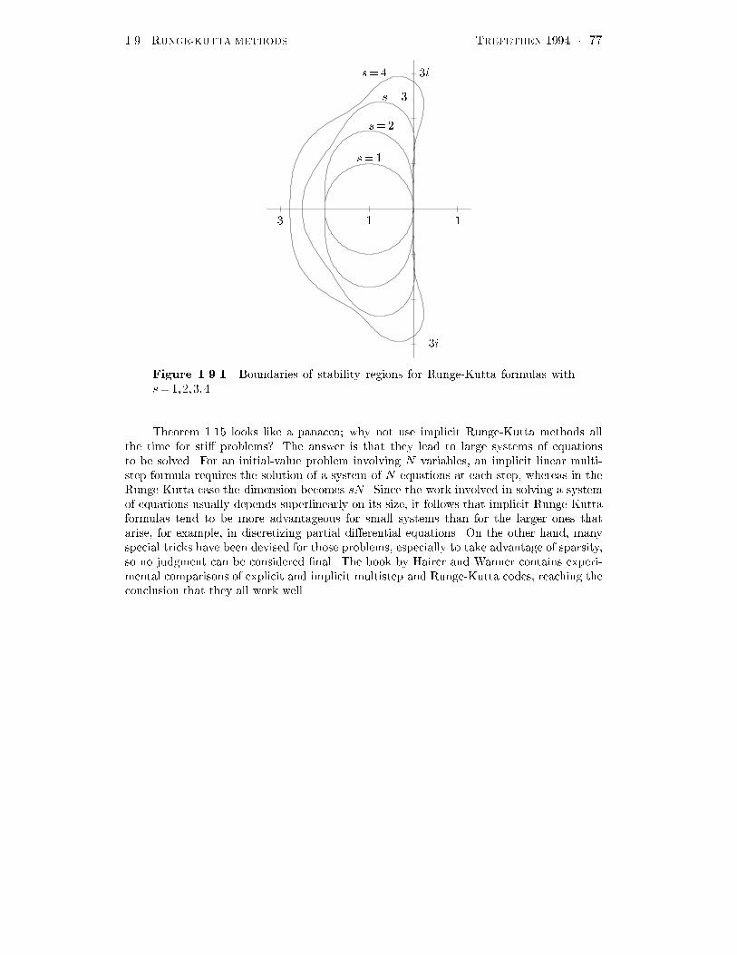
���� RUNGE�KUTTA METHODS TREFETHEN ���� �
s��
s��
s��
s��
��� ��
��i
�i
Figure ������ Boundaries of stability regions for Runge�Kutta formulas withs���������
Theorem ���� looks like a panacea� why not use implicit Runge�Kutta methods allthe time for sti� problems� The answer is that they lead to large systems of equationsto be solved� For an initial�value problem involving N variables� an implicit linear multi�step formula requires the solution of a system of N equations at each step� whereas in theRunge�Kutta case the dimension becomes sN � Since the work involved in solving a systemof equations usually depends superlinearly on its size� it follows that implicit Runge�Kuttaformulas tend to be more advantageous for small systems than for the larger ones thatarise� for example� in discretizing partial di�erential equations� On the other hand� manyspecial tricks have been devised for those problems� especially to take advantage of sparsity�so no judgment can be considered �nal� The book by Hairer and Wanner contains experi�mental comparisons of explicit and implicit multistep and Runge�Kutta codes� reaching theconclusion that they all work well�

���� NOTES AND REFERENCES TREFETHEN ���� � �
����� Notes and References
This chapter has said little about the practical side of numerical solution of ordinarydi�erential equations� One topic barely mentioned is the actual implementation of implicitmethods�the solution of the associated equations at each time step by Newton�s methodand its variants� Another gap is that we have not discussed the idea of adaptive stepsize and order control� which� together with the development of special methods for sti�problems� are the most important developments in the numerical solution of ODEs duringthe computer era� The software presently available for solving ODEs is so powerful andreliable that there is little reason other than educational to write one�s own program� exceptfor very easy problems or specialized applications� Essentially all of this software makes useof adaptive step size control� and some of it controls the order of the formula adaptivelytoo� Trustworthy codes can be found in the IMSL� NAG� and Harwell libraries� in Matlab�and in numerous other sources� The best�known programs are perhaps those developed atSandia Laboratories and the Lawrence Livermore Laboratory� which can be obtained fromthe Netlib facility described in the Preface�
Although this book does not discuss boundary�value problems for ODEs� the readershould be aware that in that area too there is excellent adaptive software� which is farmore e�cient and reliable than the program a user is likely to construct by combining aninitial�value problem solver with the idea of �shooting�� Two well�known programs arePASVA and its various derivatives� which can be found in the NAG Library� and COLSYS�which has been published in the Transactions on Mathematical Software and is availablefrom Netlib� A standard textbook on the subject is U� M� Ascher� R� M� M� Mattheij andR� D� Russell� Numerical Solution of Boundary Value Problems for Ordinary Di�erentialEquations� Prentice Hall� �����
Some applications lead to systems of di�erential equations that must be solved in con�junction with additional non�di�erential conditions� Such systems are called dierential�algebraic equations �DAEs� and have been investigated by Gear� Petzold� and manyothers� Software is available for these problems too� including a well�known program byPetzold known as DASSL�
The scale of ODEs that occur in practice can be enormous� One example of engineeringinterest arises in the simulation of VLSI circuits� where one encounters sparse sti� systemscontaining thousands or tens of thousands of variables� In such cases it is of paramountimportance to exploit the special properties of the systems� and one special method thathas been devised goes by the name of waveform relaxation� see the footnote on p� ���