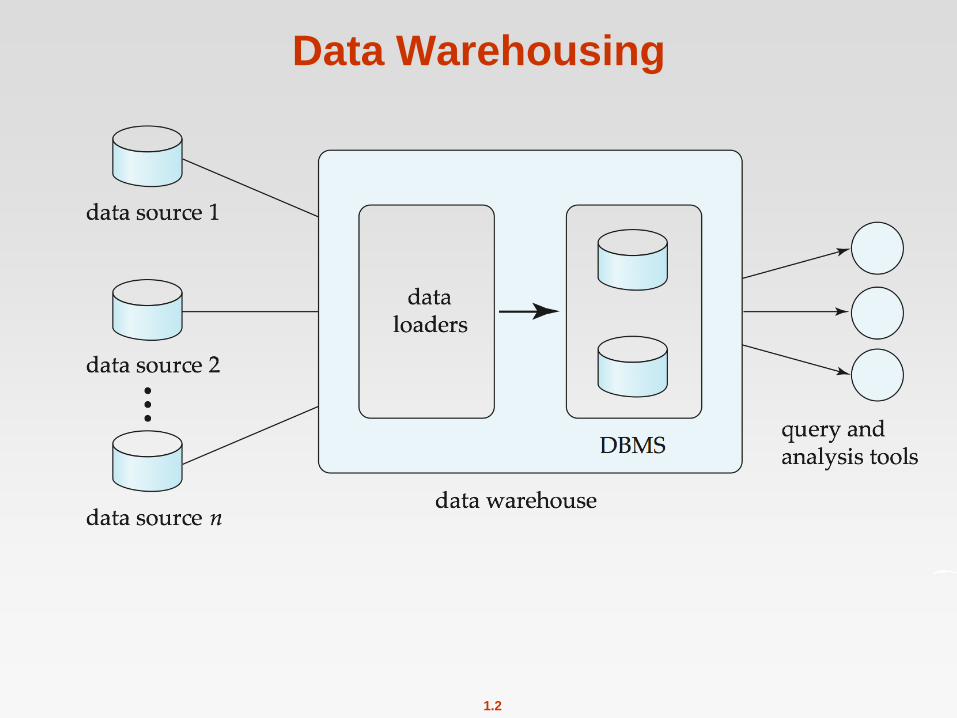
1.1

Data Warehousing

Data sources often store only current data, not historical data

Corporate decision making requires a unified view of all organizational

data, including historical data

A data warehouse is a repository (archive) of information gathered

from multiple sources, stored under a unified schema, at a single site

Greatly simplifies querying, permits study of historical trends

Shifts decision support query load away from transaction

processing systems

1.2

Data Warehousing

1.3

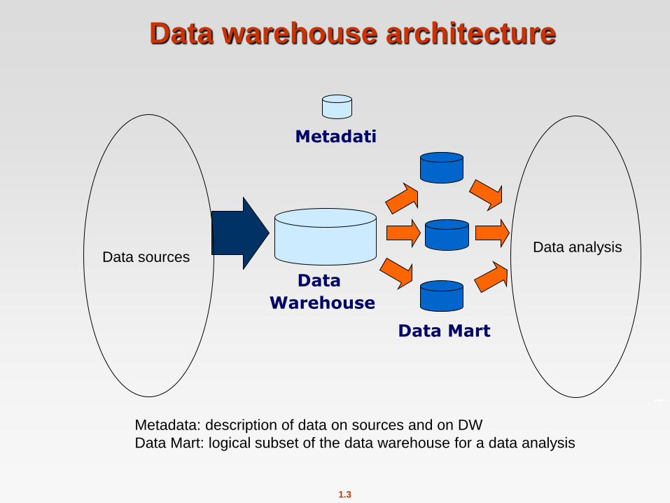
Data warehouse architecture

Metadati

Data

Warehouse

Data Mart

Data sources Data analysis

Metadata: description of data on sources and on DW

Data Mart: logical subset of the data warehouse for a data analysis

1.4

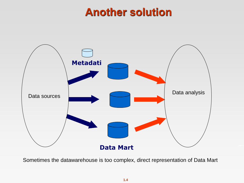
Another solution

Metadati

Data Mart

Data sources Data analysis

Sometimes the datawarehouse is too complex, direct representation of Data Mart

1.5

Design Issues

When and how to gather data

Source driven architecture: data sources transmit new

information to warehouse, either continuously or periodically

(e.g., at night)

Destination driven architecture: warehouse periodically

requests new information from data sources

Keeping warehouse exactly synchronized with data sources

(e.g., using two-phase commit) is too expensive

Usually OK to have slightly out-of-date data at warehouse

Data/updates are periodically downloaded form online

transaction processing (OLTP) systems.

What schema to use

Schema integration

1.6

More Warehouse Design Issues

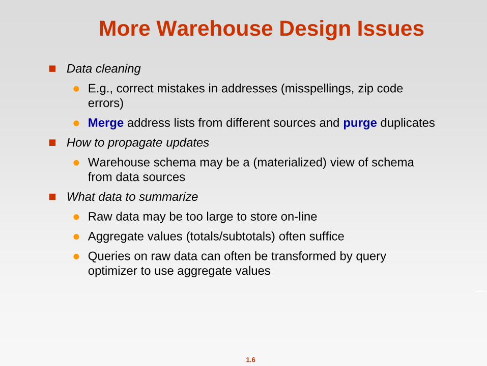
Data cleaning

E.g., correct mistakes in addresses (misspellings, zip code

errors)

Merge address lists from different sources and purge duplicates

How to propagate updates

Warehouse schema may be a (materialized) view of schema

from data sources

What data to summarize

Raw data may be too large to store on-line

Aggregate values (totals/subtotals) often suffice

Queries on raw data can often be transformed by query

optimizer to use aggregate values

1.7

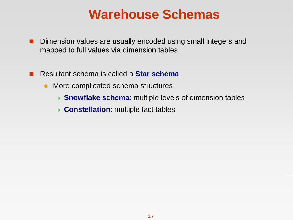
Warehouse Schemas

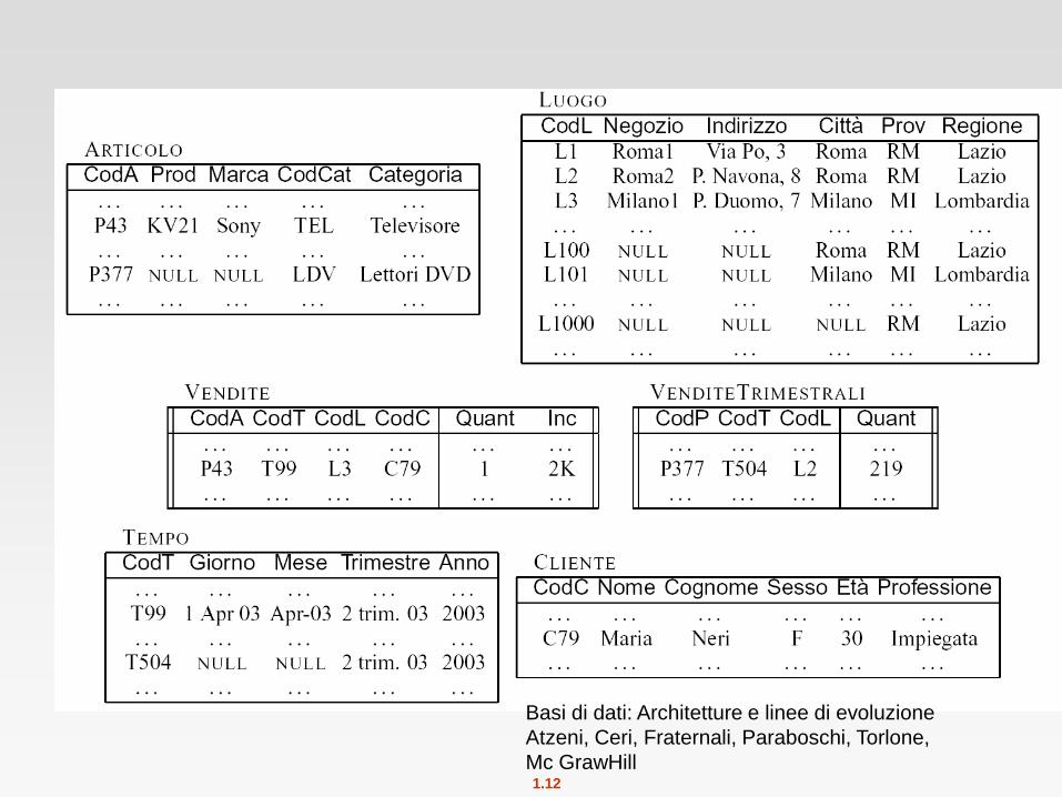
Dimension values are usually encoded using small integers and

mapped to full values via dimension tables

Resultant schema is called a Star schema

More complicated schema structures

Snowflake schema: multiple levels of dimension tables

Constellation: multiple fact tables

1.8

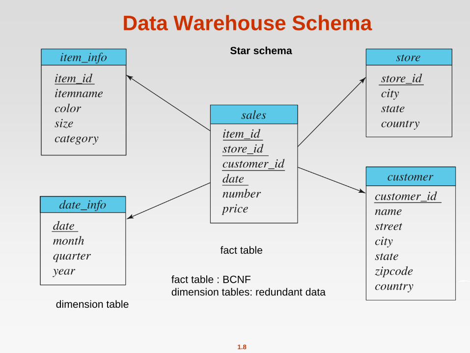
Data Warehouse Schema Star schema

fact table

dimension table

fact table : BCNF

dimension tables: redundant data

1.9

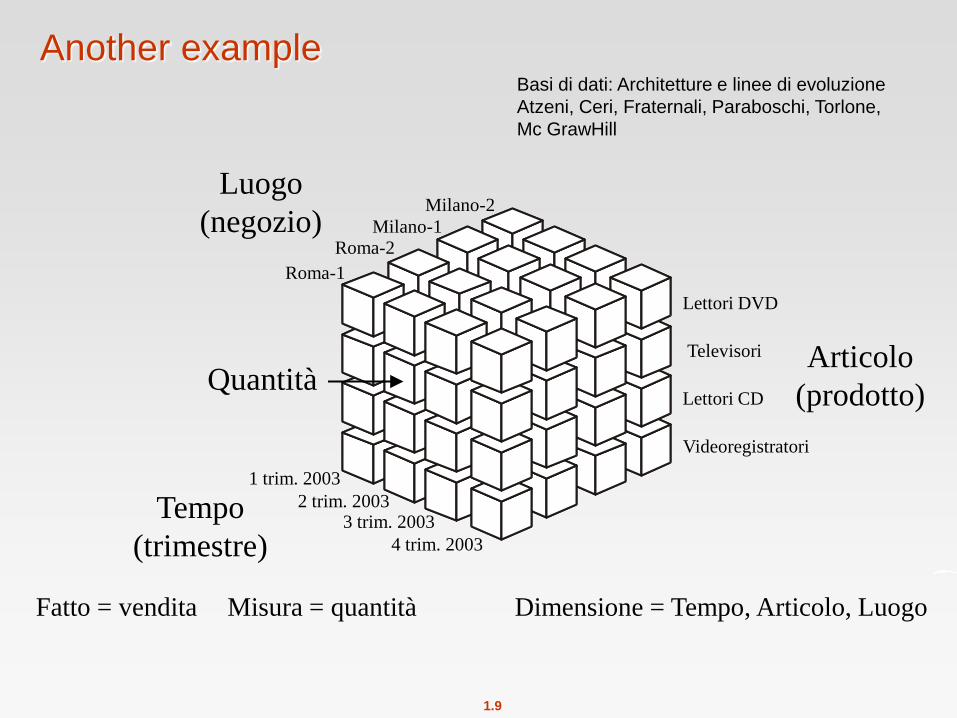
Another example

Articolo

(prodotto)

Tempo

(trimestre)

Quantità

Luogo

(negozio)

Lettori DVD

Lettori CD

Televisori

Videoregistratori

Roma-1

Roma-2 Milano-1

Milano-2

1 trim. 2003

2 trim. 2003 3 trim. 2003

4 trim. 2003

Fatto = vendita Misura = quantità Dimensione = Tempo, Articolo, Luogo

Basi di dati: Architetture e linee di evoluzione

Atzeni, Ceri, Fraternali, Paraboschi, Torlone,

Mc GrawHill

1.10

negozio

regione

provincia

città

giorno

anno

trimestre

mese prodotto

marca categoria

Luogo

Articolo

Tempo

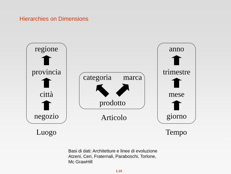
Basi di dati: Architetture e linee di evoluzione

Atzeni, Ceri, Fraternali, Paraboschi, Torlone,

Mc GrawHill

Hierarchies on Dimensions

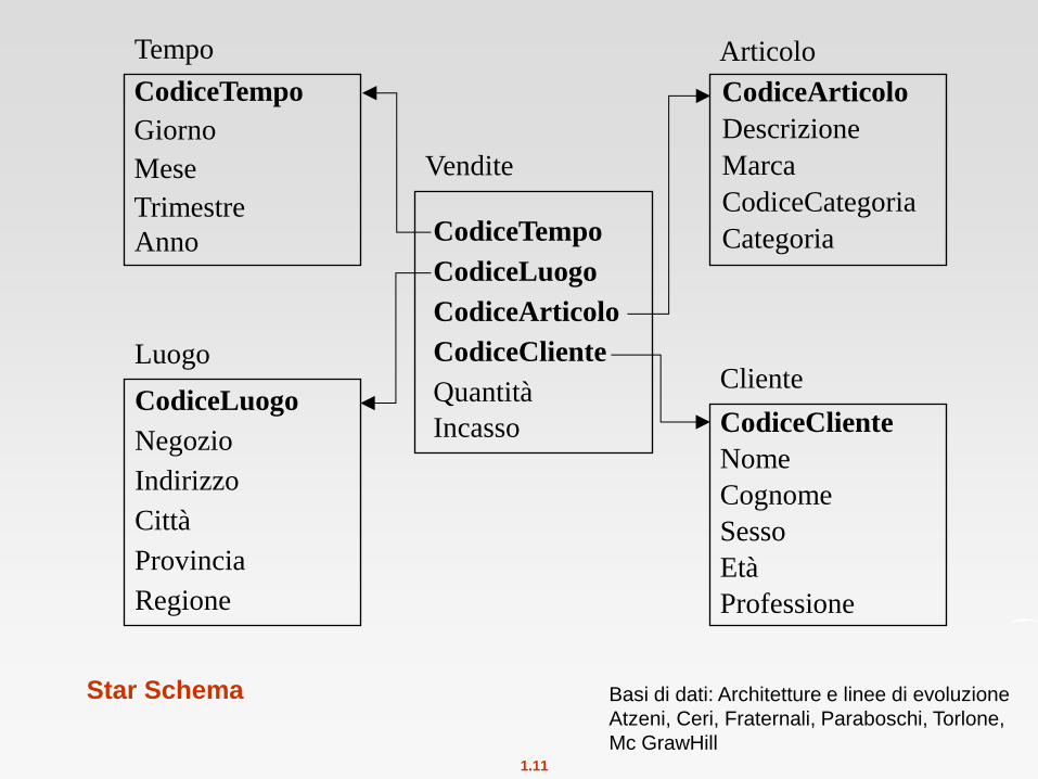
1.11

Vendite

CodiceTempo

CodiceLuogo

CodiceArticolo

CodiceCliente

Quantità

Incasso

Tempo

CodiceTempo

Giorno

Mese

Trimestre

Anno

Luogo

CodiceLuogo

Negozio

Indirizzo

Città

Provincia

Regione

Articolo

CodiceArticolo

Descrizione

Marca

CodiceCategoria

Categoria

Cliente

CodiceCliente

Nome

Cognome

Sesso

Età

Professione

Basi di dati: Architetture e linee di evoluzione

Atzeni, Ceri, Fraternali, Paraboschi, Torlone,

Mc GrawHill

Star Schema

1.12

Basi di dati: Architetture e linee di evoluzione

Atzeni, Ceri, Fraternali, Paraboschi, Torlone,

Mc GrawHill

Data Mining

These slides are a modified version of the slides of the book

“Database System Concepts” (Chapter 18), 5th Ed., McGraw-Hill,

by Silberschatz, Korth and Sudarshan.

Original slides are available at www.db-book.com

1.14

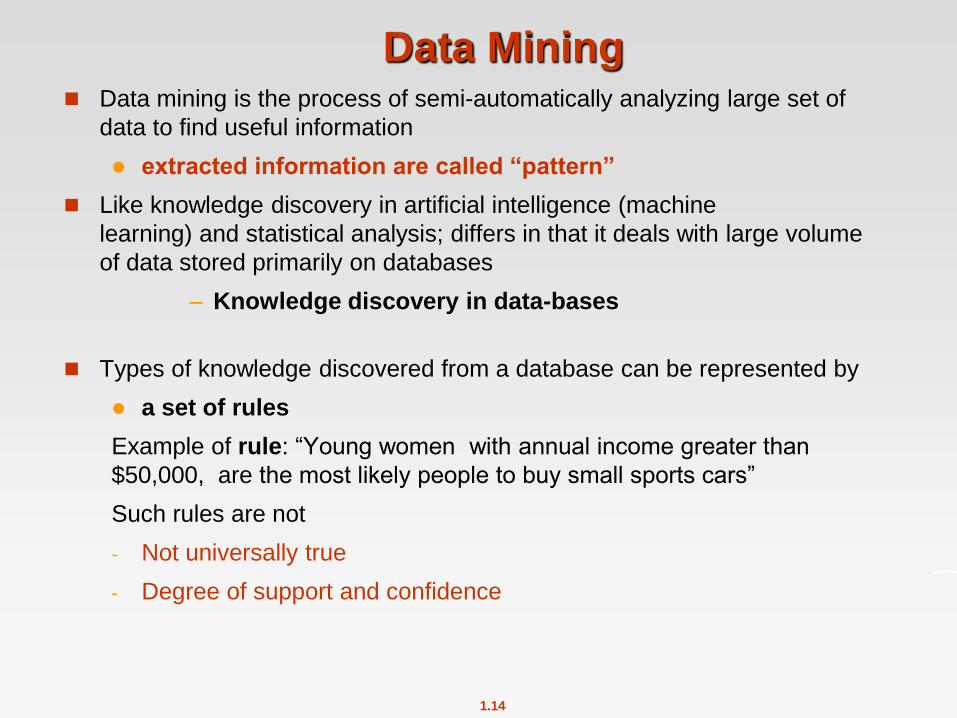
Data Mining Data mining is the process of semi-automatically analyzing large set of

data to find useful information

extracted information are called “pattern”

Like knowledge discovery in artificial intelligence (machine

learning) and statistical analysis; differs in that it deals with large volume

of data stored primarily on databases

– Knowledge discovery in data-bases

Types of knowledge discovered from a database can be represented by

a set of rules

Example of rule: “Young women with annual income greater than

$50,000, are the most likely people to buy small sports cars”

Such rules are not

- Not universally true

- Degree of support and confidence

1.15

Data Mining

Other types of knowledge are represented by

equations relating different variables each other

mechanism for predicting outcomes when the values of some

variables are known

Manual component to data mining

preprocessing data to a form acceptable to the algorithms

postprocessing of discovered patterns to find novel ones that

could be useful

Manual interaction to pick different useful types of patterns

data mining is a semi-automatic process in real life

We concentrate on the automatic aspect of mining.

We will study a few examples of patterns and we will see how they

may be automatically derived from a database

1.16

Applications of Data Mining

The most widely used applications are:

- Predication

- Association

Prediction (applications that require some form of prediction)

Example: Prediction based on past history

Credit card company: Predict if a credit card applicant poses a good credit

risk, based on some attributes of the person such as income, job type, age,

and past payment history

Rules for making the prediction are derived from the same attributes of past

and current credit-card holders, along with their observed behaviour,

such as whether they defaulted on their credit-card dues.

Other examples:

- predicting which customers may switch over to a competitor.

- predicting which people are likely to respond to promotion mail

- …..

1.17

Applications of Data Mining

Association ( applications that look for associations )

For instance:

books that tend to be bought together

If a customer buys a book, an on-line book store may suggest other

associated books.

If a person buys a book, an on-line bookstore may suggest other associated

books

If a person buys a camera, the system may suggest accessories that tend to

be bought along with cameras

Exploit such patterns to make additional sales.

1.18

Prediction techniques

Classification

Assume that items belong to one of several classes

Given past instances (called training instances) of items

along with the classes to which they belong

The problem is: given a new item, predict to which class the item belongs

The class of the new instance is not known, some attributes of the instance

can be used to predict the class

Classification can be done by finding rules that partition the given data into

disjoint groups

Classification rules: help assign new objects to classes.

1.19

Classification Rules

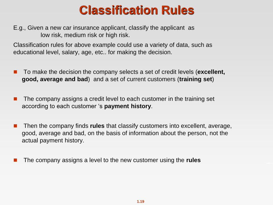
E.g., Given a new car insurance applicant, classify the applicant as

low risk, medium risk or high risk.

Classification rules for above example could use a variety of data, such as

educational level, salary, age, etc.. for making the decision.

To make the decision the company selects a set of credit levels (excellent,

good, average and bad) and a set of current customers (training set)

The company assigns a credit level to each customer in the training set

according to each customer ‘s payment history.

Then the company finds rules that classify customers into excellent, average,

good, average and bad, on the basis of information about the person, not the

actual payment history.

The company assigns a level to the new customer using the rules

1.20

Classification Rules

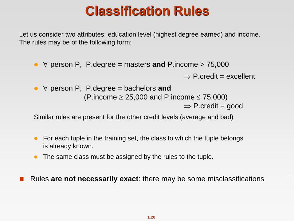
Let us consider two attributes: education level (highest degree earned) and income.

The rules may be of the following form:

person P, P.degree = masters and P.income > 75,000

P.credit = excellent

person P, P.degree = bachelors and

(P.income 25,000 and P.income 75,000)

P.credit = good

Similar rules are present for the other credit levels (average and bad)

For each tuple in the training set, the class to which the tuple belongs

is already known.

The same class must be assigned by the rules to the tuple.

Rules are not necessarily exact: there may be some misclassifications

1.21

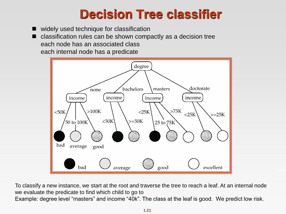
Decision Tree classifier widely used technique for classification

classification rules can be shown compactly as a decision tree

each node has an associated class

each internal node has a predicate

To classify a new instance, we start at the root and traverse the tree to reach a leaf. At an internal node

we evaluate the predicate to find which child to go to

Example: degree level “masters” and income “40k”. The class at the leaf is good. We predict low risk.

1.22

Construction of Decision-Tree classifiers

How to build a decision-tree classifier

Training set: a data sample in which the classification is already

known.

Greedy algorithm which works recursively starting at the root

and building the tree downward (top down generation of decision

trees).

Initially there is only the root. All training instances are associated

with the root.

A each node if all or almost all instances associated with the

node belongs to the same class, the node becomes a leaf node

associated with that class.

Otherwise a partitioning attribute and a partitioning condition

must be selected to create child nodes.

The data associated to each child node is the set of training

instances that satisfy the partitioning condition for that child node.

1.23

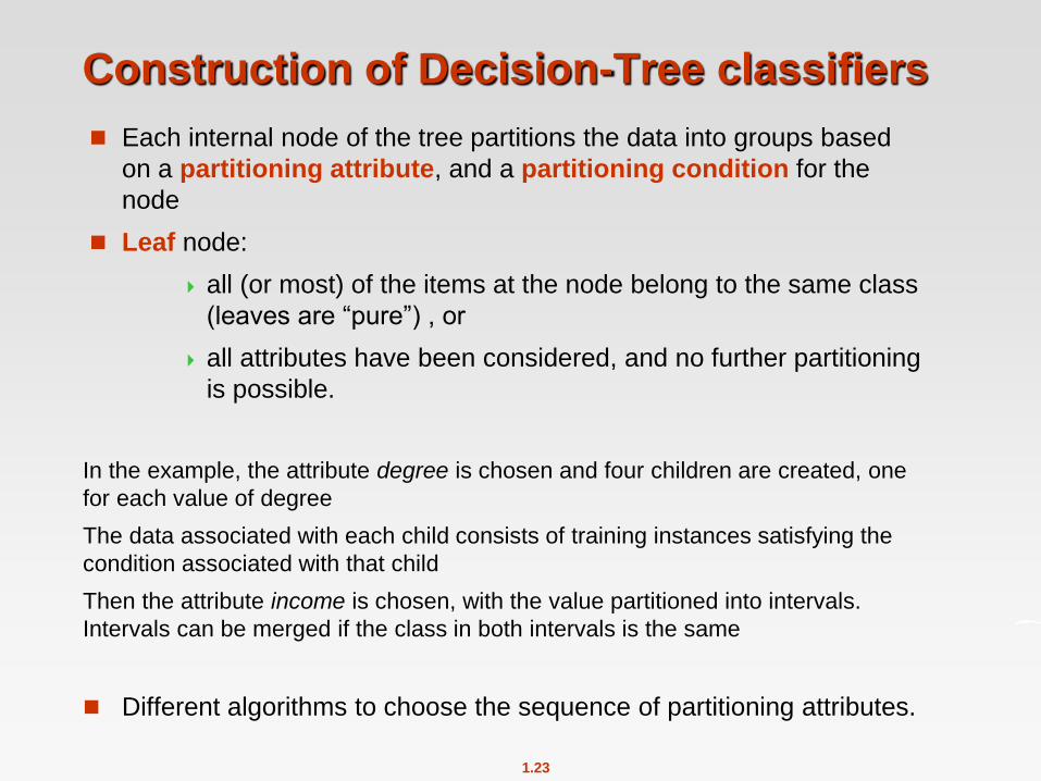
Construction of Decision-Tree classifiers

Each internal node of the tree partitions the data into groups based

on a partitioning attribute, and a partitioning condition for the

node

Leaf node:

all (or most) of the items at the node belong to the same class

(leaves are “pure”) , or

all attributes have been considered, and no further partitioning

is possible.

In the example, the attribute degree is chosen and four children are created, one

for each value of degree

The data associated with each child consists of training instances satisfying the

condition associated with that child

Then the attribute income is chosen, with the value partitioned into intervals.

Intervals can be merged if the class in both intervals is the same

Different algorithms to choose the sequence of partitioning attributes.

1.24

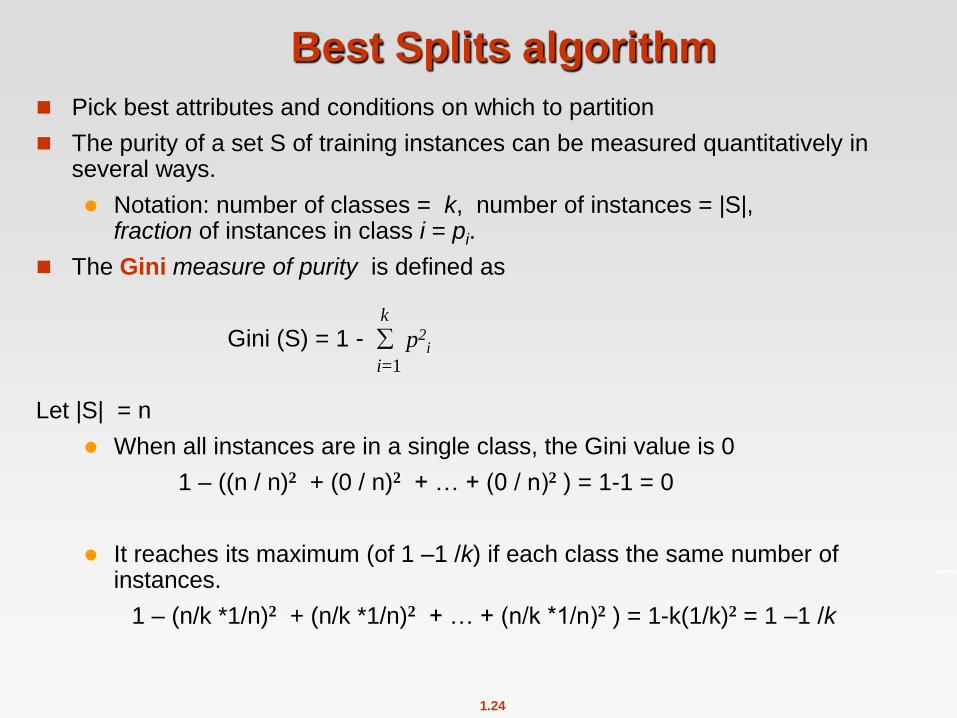
Best Splits algorithm

Pick best attributes and conditions on which to partition

The purity of a set S of training instances can be measured quantitatively in several ways.

Notation: number of classes = k, number of instances = |S|, fraction of instances in class i = pi.

The Gini measure of purity is defined as

Gini (S) = 1 -

Let |S| = n

When all instances are in a single class, the Gini value is 0

1 – ((n / n)2 + (0 / n)2 + … + (0 / n)2 ) = 1-1 = 0

It reaches its maximum (of 1 –1 /k) if each class the same number of instances.

1 – (n/k *1/n)2 + (n/k *1/n)2 + … + (n/k *1/n)2 ) = 1-k(1/k)2 = 1 –1 /k

k

i=1

p2i

1.25

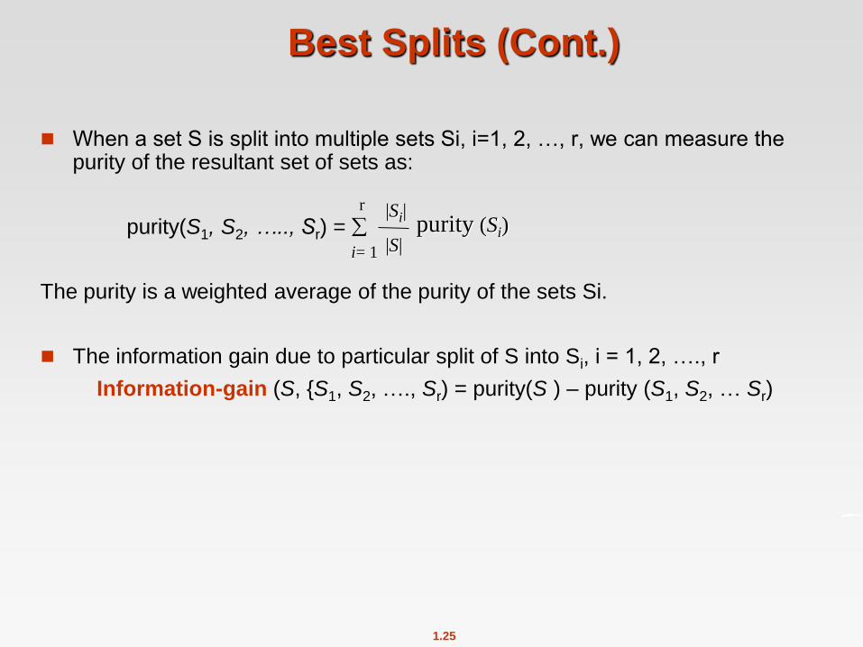
Best Splits (Cont.)

When a set S is split into multiple sets Si, i=1, 2, …, r, we can measure the purity of the resultant set of sets as:

purity(S1, S2, ….., Sr) =

The purity is a weighted average of the purity of the sets Si.

The information gain due to particular split of S into Si, i = 1, 2, …., r

Information-gain (S, {S1, S2, …., Sr) = purity(S ) – purity (S1, S2, … Sr)

r

i= 1

|Si|

|S| purity (Si)

1.26

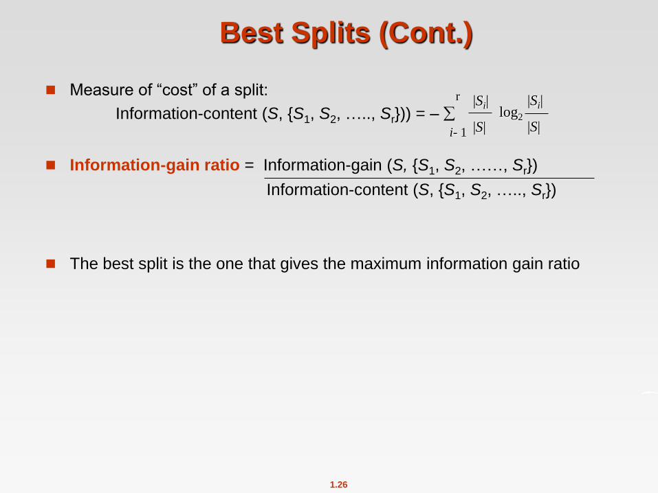
Best Splits (Cont.)

Measure of “cost” of a split:

Information-content (S, {S1, S2, ….., Sr})) = –

Information-gain ratio = Information-gain (S, {S1, S2, ……, Sr})

Information-content (S, {S1, S2, ….., Sr})

The best split is the one that gives the maximum information gain ratio

log2

r

i- 1

|Si|

|S|

|Si|

|S|

1.27

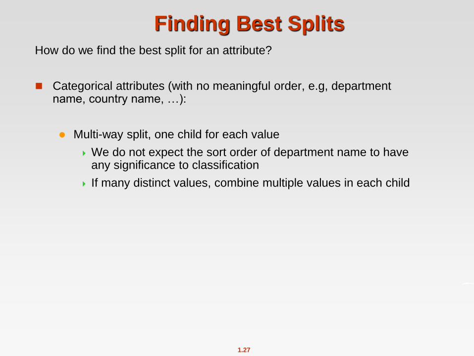
Finding Best Splits How do we find the best split for an attribute?

Categorical attributes (with no meaningful order, e.g, department name, country name, …):

Multi-way split, one child for each value

We do not expect the sort order of department name to have any significance to classification

If many distinct values, combine multiple values in each child

1.28

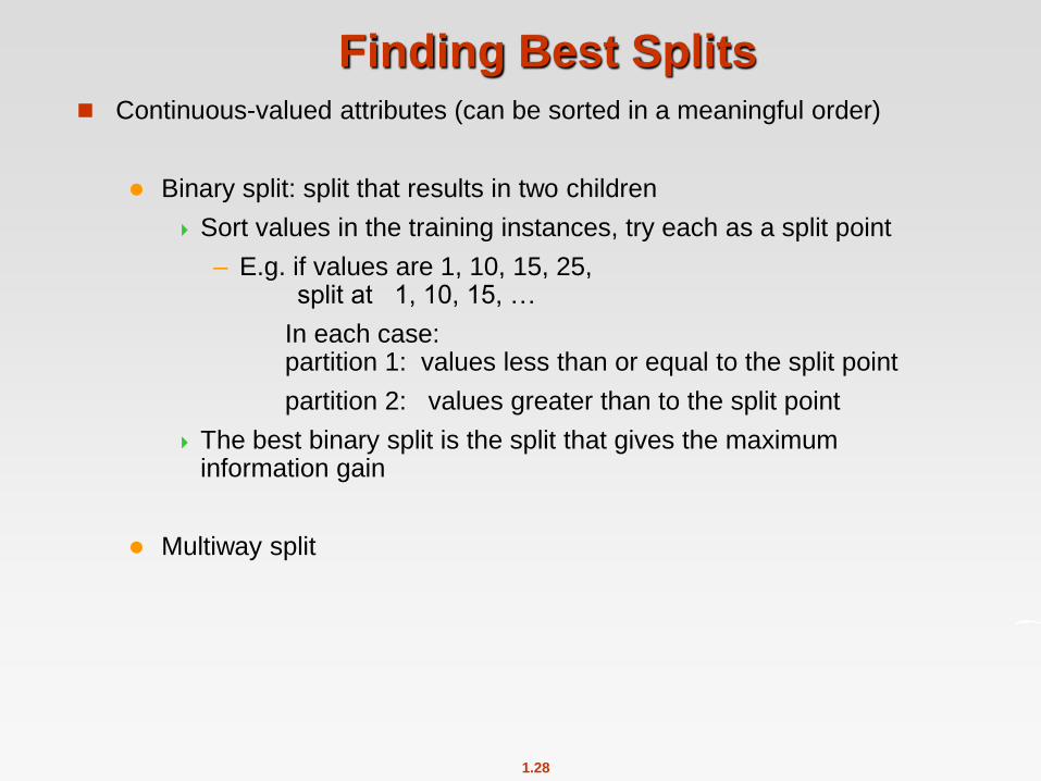
Finding Best Splits Continuous-valued attributes (can be sorted in a meaningful order)

Binary split: split that results in two children

Sort values in the training instances, try each as a split point

– E.g. if values are 1, 10, 15, 25, split at 1, 10, 15, …

In each case: partition 1: values less than or equal to the split point

partition 2: values greater than to the split point

The best binary split is the split that gives the maximum information gain

Multiway split

1.29

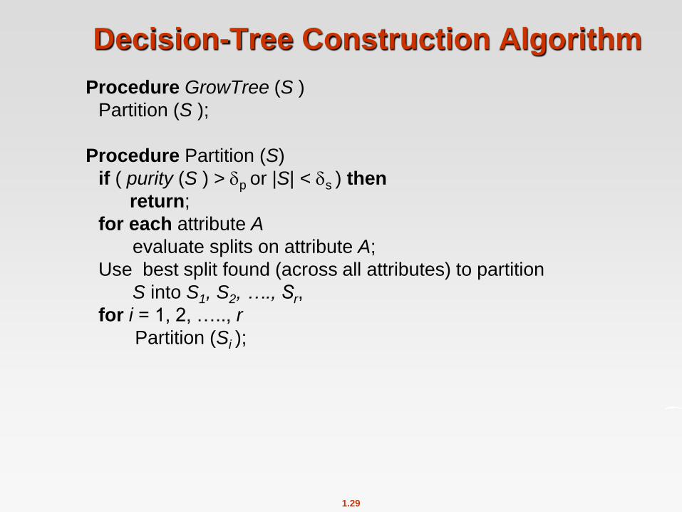
Decision-Tree Construction Algorithm

Procedure GrowTree (S )

Partition (S );

Procedure Partition (S)

if ( purity (S ) > p or |S| < s ) then

return;

for each attribute A

evaluate splits on attribute A;

Use best split found (across all attributes) to partition

S into S1, S2, …., Sr,

for i = 1, 2, ….., r

Partition (Si );

1.30

Decision-Tree Construction Algorithm

Evaluate different attributes and different partitioning conditions, and

pick the attribute and partitioning condition that results in the

maximum information gain ratio.

The same procedure applies recursively on each of the sets

resulting from the split.

If the data can be perfectly classified, the recursion stops when the

purity of a set is 0.

Often data are noisy, or a set may be so small that partitioning it

further may not be justifiable statistically.

The recursion stops when the purity of a set is sufficiently high

Parameters define cutoffs for purity and size

1.31

Other Types of Classifiers

Neural net classifiers

Bayesian classifiers

………………….

1.32

Associations

Retail shops are often interested in associations between different items that people buy.

Someone who buys bread is quite likely also to buy milk

A person who bought the book Database System Concepts is quite likely also to buy the book Operating System Concepts.

Association rules:

bread milk DB-Concepts, OS-Concepts Networks

Left hand side: antecedent, right hand side: consequent

An association rule must have an associated population; the population consists of a set of instances

E.g. each transaction (sale) at a shop is an instance, and the set of all transactions is the population

1.33

Association Rules (Cont.)

Rules have an associated support, as well as an associated confidence.

Support is a measure of what fraction of the population satisfies both the

antecedent and the consequent of the rule.

E.g. suppose only 0.001 percent of all purchases include milk and

screwdrivers. The support for the rule is milk screwdrivers is low.

Businesses are usually not interested in rules that have low support

If 50 percent of all purchases involve milk and bread then support for the rule

bread milk is high and may be worth attention

Minimum degree of attention depends on the application.

Confidence is a measure of how often the consequent is true when the

antecedent is true.

E.g. the rule bread milk has a confidence of 80 percent if 80 percent of the

purchases that include bread also include milk.

The confidence bread milk may be different from the confidence

milk bread although both have the same support

1.34

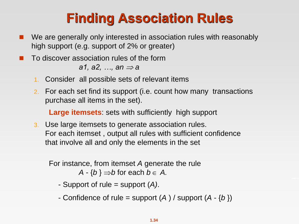
Finding Association Rules

We are generally only interested in association rules with reasonably

high support (e.g. support of 2% or greater)

To discover association rules of the form

a1, a2, …, an a

1. Consider all possible sets of relevant items

2. For each set find its support (i.e. count how many transactions

purchase all items in the set).

Large itemsets: sets with sufficiently high support

3. Use large itemsets to generate association rules.

For each itemset , output all rules with sufficient confidence

that involve all and only the elements in the set

For instance, from itemset A generate the rule

A - {b } b for each b A.

- Support of rule = support (A).

- Confidence of rule = support (A ) / support (A - {b })

1.35

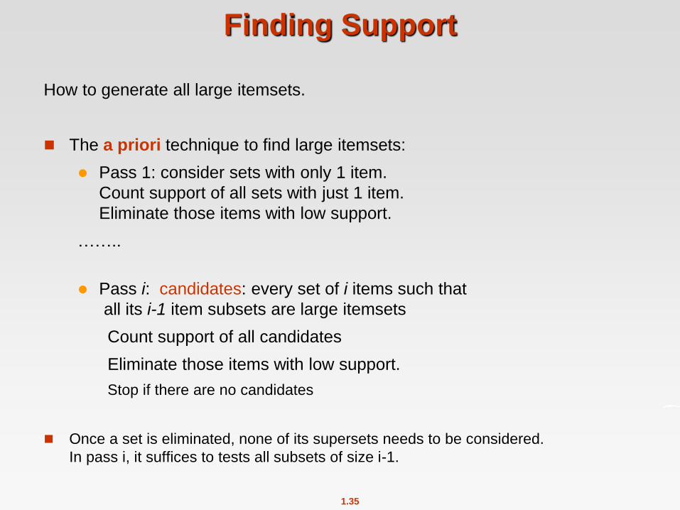
Finding Support

How to generate all large itemsets.

The a priori technique to find large itemsets:

Pass 1: consider sets with only 1 item.

Count support of all sets with just 1 item.

Eliminate those items with low support.

……..

Pass i: candidates: every set of i items such that

all its i-1 item subsets are large itemsets

Count support of all candidates

Eliminate those items with low support.

Stop if there are no candidates

Once a set is eliminated, none of its supersets needs to be considered.

In pass i, it suffices to tests all subsets of size i-1.

1.36

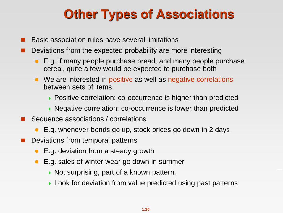
Other Types of Associations

Basic association rules have several limitations

Deviations from the expected probability are more interesting

E.g. if many people purchase bread, and many people purchase cereal, quite a few would be expected to purchase both

We are interested in positive as well as negative correlations between sets of items

Positive correlation: co-occurrence is higher than predicted

Negative correlation: co-occurrence is lower than predicted

Sequence associations / correlations

E.g. whenever bonds go up, stock prices go down in 2 days

Deviations from temporal patterns

E.g. deviation from a steady growth

E.g. sales of winter wear go down in summer

Not surprising, part of a known pattern.

Look for deviation from value predicted using past patterns