
Chapter 1 Elementary kinetic theory of...
88
ME 591, Non‐equilibrium gas dynamics, Alexey Volkov 1 Chapter 1 Elementary kinetic theory of gases 1.1. Introduction. Molecular description of gases 1.2. Molecular quantities and macroscopic gas parameters 1.3. Gas laws 1.4. Collision frequency. Free molecular, transitional, and continuum flow regimes 1.5. Transfer of molecular quantities 1.6. Transfer equation 1.7. Diffusion, viscous drag, and heat conduction 1.8. Appendix: Probability and Bernoulli trial
Transcript of Chapter 1 Elementary kinetic theory of...

ME 591, Non‐equilibrium gas dynamics, Alexey Volkov 1
Chapter 1 Elementary kinetic theory of gases
1.1. Introduction. Molecular description of gases1.2. Molecular quantities and macroscopic gas parameters 1.3. Gas laws1.4. Collision frequency. Free molecular, transitional, and continuum flow regimes1.5. Transfer of molecular quantities1.6. Transfer equation1.7. Diffusion, viscous drag, and heat conduction1.8. Appendix: Probability and Bernoulli trial

ME 591, Non‐equilibrium gas dynamics, Alexey Volkov 2
1.1. Introduction. Molecular description of gases Subject of kinetic theory. What are we going to study? Historical perspective Hypothesis of molecular structure of gases Sizes of atoms and molecules Masses of atoms and molecules Properties of major components of atmospheric air and other gases Length and time scale of inter‐molecular collisions Characteristic distance between molecules in gases Density parameter. Dilute and dense gases Purpose of the kinetic theory Chaotic motion of molecules. Major approach of the kinetic theory Specific goals of the kinetic theory Applications of the kinetic theory and RGD

ME 591, Non‐equilibrium gas dynamics, Alexey Volkov 3
1.1. Introduction. Molecular description of gasesSubject of kinetic theory. What are we going to study?
Kinetic theory of gases is a part of statistical physics where flows of gases are considered onthe molecular level, i.e. on the level of individual molecules, and described in terms ofchanges of probabilities of various states of gas molecules in space and time based onknown laws of interaction between individual molecules.Word “Kinetic” came from a Greek verb meaning "to move“ or “to induce a motion.”
Rarefied gas dynamics (RGD) is often used as a synonymous of the kinetic theory of gases. Inthe narrow sense, the kinetic theory focuses on the general methods of statisticaldescription of gas flows, while the rarefied gas dynamics focuses on solutions of practical gasdynamics problems based on methods of kinetic theory.
Non‐equilibrium gas dynamics combines methods of rarefied gas dynamics and continuumgas dynamics for description of non‐equilibrium gas flows.
Direct simulation Monte Carlo (DSMC) method is a stochastic Monte Carlo method forsimulation of dilute gas flows on the molecular level. To date, DSMC is the state‐of‐the‐artnumerical tool for the majority of applications in the kinetic theory of gases and rarefied gasdynamics.
Monte Carlo (MC) method is a general numerical method for a variety of mathematicalproblems based on computer generation of (pseudo) random numbers and probabilitytheory.

ME 591, Non‐equilibrium gas dynamics, Alexey Volkov 4
1.1. Introduction. Molecular description of gasesHistorical perspective
Historically, kinetic theory of gases evolves from the molecular theory of heat, which derives,e.g., gas laws from thermal (chaotic) motion of individual gas molecules.
The breakthrough was performed by Ludwig Boltzmann, the fatherof the kinetic theory, who derived the Boltzmann kinetic equation(Chapter 3), a equation that describes any dynamic process in gasesin terms of motion and interaction of gas molecules.The kinetic theory, however, attracted huge attention only in themiddle of XX century as a practical tool for studying low‐density gasflows in aerospace applications.Applications of the approach developed by L. Boltzmann go farbeyond the kinetic theory of gases. Numerous generalizations of hisequation are used in various branches of physics. For example, theBoltzmann transport equation (BTE) is used in the solid‐statephysics to describe transport properties (e.g., thermal conductivity)of materials with crystalline lattices.L. Boltzmann is famous not only for his kinetic equation. He wasone of founders of the statistical physics in general and establisheda relationship between entropy and probability of states of aphysical system , log .
Ludwig Eduard Boltzmann(1844 –1906)
Austrian physicist and philosopher

ME 591, Non‐equilibrium gas dynamics, Alexey Volkov 5
1.1. Introduction. Molecular description of gasesHypothesis of molecular structure of gases
Kinetic theory of gases is a part of statistical physics where flows of gases are considered on themolecular level and described in terms of changes of probabilities of various states of gasmolecules in space and time based on known laws of interaction between individual molecules.The starting point of the kinetic theory is the hypothesis of the molecular structure of gases:Any gas consists of distinct individual particles – molecules. Modern kinetic theory considers notonly electrically neutral and chemically inert monatomic gases (e.g., noble gases), but also gasescomposed of charged ions and electrons (plasma), molecules (molecular gases) and chemicallyreactive gas mixtures, as well as granular gases composed of macroscopic solid particles.
Sizes of atoms and molecules
Molecules consist of one or multiple atoms. Every atom has a nucleus that is surrounded
by a “cloud” of negatively charged electrons. A nucleus consist of nucleons: positively
charged protons and electrically neutralneutrons.
The characteristic diameter of the nucleus isabout 1 Fermi (10‐15 m), while the diameterof the electron cloud is about 1 Angstrom (Å,10‐10 m).
10‐15 m
10‐10 m

ME 591, Non‐equilibrium gas dynamics, Alexey Volkov 6
1.1. Introduction. Molecular description of gases
According to quantum mechanics, atomsdo not have any "natural" size, becauseelectrons surrounding nuclei cannot beconsidered as point masses. Everyelectron (or electron pair) ischaracterized by an electron orbital,which is a mathematical functiondescribing the probability to findelectron in different points around thenucleus.
Individual atoms compose a molecule when chemicalbonds form due to the overlap of electron orbitalsbelonging to different atoms.
Therefore, the distance between neighbor atoms in amolecule (bond length) has an order of the atomicdiameter.
Sizes of molecules of diatomic (O2, N2) and triatomic(CO2, water vapor) gases have the same order ofmagnitude as the sizes of individual atoms.
N2 H2O
N N
1.0975 Å
Bond length

ME 591, Non‐equilibrium gas dynamics, Alexey Volkov 7
1.1. Introduction. Molecular description of gasesIn different applications, the sizes of atoms and molecules can be chosen based on differentconsiderations in order to match the most important (in the particular field/problem)experimental characteristics.In the kinetic theory, the size of atoms and molecules is usually characterized by so‐calledgaskinetic or kinetic diameters , which are chosen to match values of gas viscosity predictedby a theory to experimentally measured values.
Masses of atoms and molecules Mass of a molecule is the sum of masses of individual atoms composing molecules. Mass of an atom is a sum of masses of the nucleus and electrons. The mass of a nucleus is not precisely equal to the sum of masses of individual nucleons
because of relativistic effects (transformation of mass into binding energy betweennucleons).
The rest mass of a proton is = 1.67×10⁻²⁷ kg = 1.007 Da The rest mass of an electron is 9.11×10⁻³¹ kg = 5.486×10⁻⁴ Da ~ 0.001 of proton mass,
so the major mass of an atom is concentrated in its nucleus. Since masses of atoms and molecules are small in kg, it is convenient to measure them in
specific atomic mass units. The unified atomic mass unit (symbol u) or Dalton (symbol Da) isthe standard unit that is used for measuring masses on the atomic or molecular scale. One uis approximately equal to the mass of one nucleon (either a proton or neutron).

ME 591, Non‐equilibrium gas dynamics, Alexey Volkov 8
1.1. Introduction. Molecular description of gasesOne unified atomic mass unit is defined as one twelfth of the mass of an unbound neutral atomof carbon‐12 (C12) in its nuclear and electronic ground state, and has a value of
1 u = 1 Da = = = 1.660539040×10⁻²⁷ kg.
The amu without the "unified" prefix is an obsolete unit that was based on oxygen. Manysources still use the term "amu," but now define it in the same way as u (i.e., based on C12). Inthis sense, the majority of uses of the terms "atomic mass units" and "amu" today actually referto the unified atomic mass unit.The definition of u is related to the definition of a mole. Themole (symbolmol) is the amount ofsubstance, which contains as many elementary entities (particles) as there are atoms in 12 g ofC12. The notion of mole is used to count the number of particles, not the mass. When the moleis used, the elementary entities must be specified and may be atoms, molecules, ions, electrons,other particles, or specified groups of such particles. The number of particles in 1 mole is theuniversal constant that relates the number of entities to the amount of substance for anysample and called the Avogadro constant
6.022140857×10²³ mol−1 (entities per mole).
Themolar mass,molecular mass ormolecular weight of a species is the mass of its one mole
where is the mass of an individual particle. The relative atomic mass (atomic weight) hastraditionally been a relative scale, but currently it is measured in u.

ME 591, Non‐equilibrium gas dynamics, Alexey Volkov 9
1.1. Introduction. Molecular description of gasesLet's assume that we know the molar mass of a gas in gram. What is the mass of individualmolecule of this gas in Da?
Da g
12
g12 g / g
12
g
Thus, the mass of a molecule in Da is numerically equal to the molar mass in gram.
Properties of major components of atmospheric air and other gasesSpecies
Nitrogen N2
Oxygen O2
Carbon dioxide CO2
Carbon monoxide CO
Helium He
Neon Ne
Argon Ar
Krypton Ke
Xenon Xe
Carbon vapor C
Silicon vapor Si
m kg
Volumefraction in air

ME 591, Non‐equilibrium gas dynamics, Alexey Volkov 10
1.1. Introduction. Molecular description of gasesSpecies of the atmospheric air

ME 591, Non‐equilibrium gas dynamics, Alexey Volkov 11
1.1. Introduction. Molecular description of gasesLength and time scale of inter‐molecular collisions
Interatomic forces are short‐range and molecules strongly interact with each other only if thedistance between them is in the order of the molecular size. Then the length scale ofintermolecular collisions, , i.e. the characteristic length of a path of a molecule duringcollision, is in the order of the kinetic diameter of molecules
~ ~1Å.As we will see later on, the characteristic chaotic velocity of gas molecule 3 has theorder of the sound speed or ( is the gas constant, is the isentropic index). With typicalvalues of ~ 300 J/K/kg and ~ 300 K , ~ 300 m/s. Then the time scale of intermolecularcollisions, , i.e. the characteristic duration of the binary collision, is equal to
~ ~10 s 1ps
The kinetic theory studies processes is gases evolving on length and time scales that are muchlarger that the length and time scale of an individual collision. For this reason, we willsystematically neglect the displacement of molecules during collision and treat any collision asan instant change of molecular velocities taking place in a given point.
Individual interactionbetween a pair of gasmolecules is called thebinary collision.
No interaction No interaction
Collision

ME 591, Non‐equilibrium gas dynamics, Alexey Volkov 12
1.1. Introduction. Molecular description of gasesCharacteristic distance between molecules in gases
Number density of a gas is the number of molecules in a unite volume =1/m3. If we knowthen the number of molecules in volume of a homogeneous gas is equal to .Let’s assume that a gas has number density is known and calculate (estimate) thecharacteristic (average, mean) distance (spacing) between molecules ?If a unit volume (1 m3) contains molecules, then in average one molecule occupies the volume1/ , which we can consider as a cube of size 1/ . Since in every such “cell” in average wehave only one molecule, then the average distance between neighbor molecules is equal to thedistance between “cell” centers, i.e.
1/
1/× ×
1/
1/
1 m3

ME 591, Non‐equilibrium gas dynamics, Alexey Volkov 13
1.1. Introduction. Molecular description of gasesExample: The number of molecules in 1 cubic meter of an ideal gas (e.g., atmospheric air) atstandard conditions (pressure 101325 Pa or 1 atm, temperature 273.15 K or 0o C) is called theLoschmidt constant and is equal to
2.6868 · 10 1/m
Then the average distance between molecules is equal to ̅ 1/ ~3.3 nm≫ .
Density parameter. Dilute and dense gasesLet's represent in the form
1,
where is called the density parameter. The density parameter characterizes thevolume occupied by molecules themselves. If every molecule is viewed as a sphere of diameter, then the volume fraction of molecules (fraction of a unit volume occupied by molecules)
6 ~ .
Dilute gas is a gas, where ≪ 1, i.e. the fraction of volume occupied by molecules is negligiblecompared to the volume occupied by the gas. In the dilute gas, distance between molecules ismuch larger than the size of molecules or length scale of collisions , so that at everyparticular time, the majority of molecules move without interaction with other molecules. Wewill study the kinetic theory of only dilute gases.

ME 591, Non‐equilibrium gas dynamics, Alexey Volkov 14
1.1. Introduction. Molecular description of gasesIt will be shown later on (see Section 1.4) that in dilute gases, it is sufficient to account for onlybinary collisions between molecules, while collective interactions between multiple moleculesare so infrequent that they can be completely neglected.
At standard conditions in Earth's atmosphere, 3.7 · 10 2.6868 · 10 1.4 · 10 ,
so that the atmospheric air can be considered as a dilute gas in the full range of pressuresspecific for Earth's atmosphere. However, if density increase in 10‐100 time (up to pressure of10‐100 atm at temperature 0o C), then effects of the dense gas become important.The kinetic theory is mostly successful in description of properties of dilute gases.
Dense gas is a gas, where ~1, and distance between moleculesis about the size of molecules . Two major effects in dense gases: Smaller compressibility: The degree of compressibility is
constrained by the volume fraction of molecules. Collective interactions between molecules: Every individual
molecule interacts simultaneously with multiple surroundingmolecules.
These effects make the dense gases similar to liquids. The dense gasis a "boundary" state of matter between "true" (dilute) gases andliquids.

ME 591, Non‐equilibrium gas dynamics, Alexey Volkov 15
1.1. Introduction. Molecular description of gasesIn thermodynamics, the model of an ideal gas corresponds to themodel of dilute gas in the kinetic theory.Any deviation from the ideal gas behavior is called the real‐gaseffect.Real‐gas effects exhibit themselves, in particular, in deviation fromthe ideal gas laws (see Section 1.3):
at , (Here , , and are the pressure, volume, and number ofmolecules, is the Boltzmann constant). In real gases, pressurerises with decreasing faster than it is predicted for the ideal gas.
1 bar = 105 Pa ~ 1 atm

ME 591, Non‐equilibrium gas dynamics, Alexey Volkov 16
1.1. Introduction. Molecular description of gasesPurpose of the kinetic theory
Kinetic theory of gases is a part of statistical physics where flows of gases are considered on themolecular level and described in terms of changes of probabilities of various states of gasmolecules in space and time based on known laws of interaction between individual molecules.
The major purpose of the kinetic theory is to derive mathematical description of a gas flowfrom a law of interaction between individual gas molecules.
As a result, in kinetic theory, any gas property (e.g. viscosity) or parameter (e.g. pressure), iscompletely defined by physical parameters of intermolecular interaction law and parametersof motion of individual molecules (velocity, etc.).
Kinetic theory itself, however, cannot predict the intermolecular interaction laws. These lawsmust be establish by the methods of quantum mechanics or experimentally.
Input:Law of interaction between molecules
Output:Any flow property

ME 591, Non‐equilibrium gas dynamics, Alexey Volkov 17
1.1. Introduction. Molecular description of gasesChaotic motion of molecules. Major approach of the kinetic theory
Kinetic theory of gases is a part of statistical physics where flows of gases are considered on themolecular level and described in terms of changes of probabilities of various states of gasmolecules in space and time based on known laws of interaction between individual molecules.
In the majority of practical problems, the number of individual molecules in gas flows is toolarge in order to trace every individual molecule.Example: The number of molecules in 1 cubic meter of atmospheric air) at standard conditions
2.6868 · 10 1/m .
If we want to trace every molecule in such volume, then we need to store in computer memory6 real numbers (3 coordinates, 3 velocity component for every molecule) and to use
6 82 ~10 GByte.of computer memory. This is an unviable approach even in the very long run!
Too manymolecules

ME 591, Non‐equilibrium gas dynamics, Alexey Volkov 18
1.1. Introduction. Molecular description of gasesThe major foundation of the kinetic theory is the well‐established experimental fact thatindividual molecules in gases move chaotically, i.e. individual molecules in any small volume of agas flow have vectors of velocity that are different from each other in magnitude and direction.
Then one can use the methods of mathematical theory of probability and statistics in order tostudy distributions of chaotic velocities of gas molecules without considering motion of allmolecules composing a gas flow.The major approach of the kinetic theory is to consider coordinates, velocities (and, may be otherparameters describing internal motion of individual atoms within molecules) as randomvariables. Such statistical approach allows one to study systems composed of extremely largenumber of gas molecules without explicit restrictions on .
Chaotic motion of molecules is also calledthermal motion since, as will see later on,temperature is a measure of magnitudeof chaotic velocities of individualmolecules

ME 591, Non‐equilibrium gas dynamics, Alexey Volkov 19
1.1. Introduction. Molecular description of gases
Soot nanocluster Atmosphere of Io
3640 km
As a result, Kinetic theory has no intrinsic restrictions on the number of molecules in the flow and flow
length scale. It can be used for problem from nano‐ to planetary scale.

ME 591, Non‐equilibrium gas dynamics, Alexey Volkov 20
1.1. Introduction. Molecular description of gasesSpecific goals of the kinetic theory
To provide a kinetic foundation of the continuum gas dynamics, i.e. to derive gas dynamicsequations from equations of motion of individual molecules
To generalize continuum gas dynamics, i.e. to develop approaches for mathematicaldescriptions of gas flows in conditions when continuum gas dynamics is not applicable
Examples of conditions when the kinetic description of gas flows in required: Low‐density flow
Small‐scale flow
Fast, non‐equilibrium flowsand flows with highgradients of gas parameters(evaporation, shock waves)

ME 591, Non‐equilibrium gas dynamics, Alexey Volkov 21
1.1. Introduction. Molecular description of gasesApplications of the kinetic theory of gases and RGD
Aerospace applications: Flows in upper atmosphere and in vacuum
Vacuum devices, microchannels, microparticles and clusters
Satellites and spacecraftson LEO and in deep space
Re‐entry vehicles inupper atmosphere
Nozzles and jetsin space environment
Microchannels Microparticlesand clusters
Soot clusters
Si waferHD
Microelectronic devices and MEMS
Vacuum pumps, vacuum chambers

ME 591, Non‐equilibrium gas dynamics, Alexey Volkov 22
1.1. Introduction. Molecular description of gasesApplications of the kinetic theory of gases and RGD
Fast, non‐equilibrium gas flows (laser ablation, evaporation, vapor deposition)
Natural phenomena in planetary science and astrophysicsDynamics of upper planetary atmospheres:Solar system, exoplanets
Global atmospheric evolution of distant bodies in the solar systems (Io, Enceladus, Pluto, etc.)
HD189733b
Io Comet 67/P
Atmospheres of comets

ME 591, Non‐equilibrium gas dynamics, Alexey Volkov 23
1.2. Molecular quantities and macroscopic gas parameters Macroscopic gas parameters in continuum mechanics Molecular quantities Macroscopic gas parameters as volume‐averaged molecular quantities Macroscopic gas velocity and velocity of chaotic motion of molecules Total and internal energies Restrictions of the continuity hypothesis

ME 591, Non‐equilibrium gas dynamics, Alexey Volkov 24
1.2. Molecular quantities and macroscopic gas parametersIn Section 1.1 we discussed two major specific goals of the kinetic theory: To provide a kinetic foundation of the continuum gas dynamics, i.e. to derive gas dynamics
equations from equations of motion of individual molecules To generalize continuum gas dynamics, i.e. to develop approaches for mathematical
descriptions of gas flows in conditions when continuum gas dynamics is not applicableIn order to achieve these goals we, first of all, need to establish a relationship between physicalquantities assigned to individual gas molecules and macroscopic gas parameters. Suchparameters should have the same meaning as gas parameters in continuum mechanics.
Macroscopic gas parameters in continuum gas dynamicsIn continuum gas dynamics, the molecular structure of a gas is neglected. The gas is viewed as amatter that is continuously distributed and fills the entire region of space it occupies. Variousphysical quantities associated with the this matter (continuum) are characterized by continuousfields of densities of mass, momentum, energy, etc.
, , density of the energy in point , = J/m3;
, , gas energy in the infinitesimal volume around point ;The gas energy in a finite volume is equal to
, .

ME 591, Non‐equilibrium gas dynamics, Alexey Volkov 25
1.2. Molecular quantities and macroscopic gas parametersFrom the point of view of molecular structure of gases, any gas is a system of molecules. Thenany macroscopic gas quantity is a function of corresponding molecular quantities associatedwith individual gas molecules. For example, the total energy of the gas in volume is just a sumof energies of individual molecules.
Molecular quantities Let's denote different molecules by the subscript ( 1,2, …) and assume that every moleculeis a point mass particle of mass . The state of molecule at time is completely defined by itsposition vector and velocity vector . We can also introduce a number of other physicalquantities that are associated with molecule .
1, quantity that serves to count the number of molecules;, molecule mass;
, linear momentum of molecule;
/2, translational (kinetic) energy of molecule;, angular momentum of molecule;
Any such physical quantity Φ Φ , , associated with anindividual gas molecule is called themolecular quantity.One can introduce many different molecular quantities, but themost important of them correspond to physical quantities thatconserve their values in a closed system of molecules, i.e. asystem, where molecules are not affected by any external force.

ME 591, Non‐equilibrium gas dynamics, Alexey Volkov 26
1.2. Molecular quantities and macroscopic gas parametersRepresentative elementary volume and continuity hypothesis
Macroscopic gas parameters (macroparameters) can be introduced as averaged values ofcorresponding individual molecular quantities. Their definition is based on the hypothesis ofexistence of a representative elementary volume (R.E.V.).Representative elementary volumeΔ around some point in the flow is such a volume that Linear size of this volume Δ is negligibly small compared to the flow length scale , Δ ≪
,so that we can neglect inhomogeneity of the gas flow inside Δ and mathematicallyconsider Δ as an infinitesimal volume.
This volume contains very large number of molecules, Δ ≫ 1, so that the total value of anyphysical quantity for the whole system of molecules inside this volume exhibit negligiblefluctuations because of the chaotic motion of molecules.
Δ
If such R.E.V. can be introduced in any point of the flow field,then we say that the hypothesis of existence of R.E.V. issatisfied. It is also called the continuity hypothesis, sincecontinuum mechanics is valid only if R.E.V. exist everywhere.
Δ
∆

ME 591, Non‐equilibrium gas dynamics, Alexey Volkov 27
1.2. Molecular quantities and macroscopic gas parameters
(1.2.1)
(1.2.2)
(1.2.3)
Φ Φ
Macroscopic gas properties as volume‐averaged molecular quantitiesIf R.E.V. exists in point , then we can introduce the macroscopic gas parameter Φ of physicalquantity Φ in this point as a volume‐averaged value of corresponding molecular quantitiesΦ , , for all molecules in R.E.V
Φ ,1Δ Φ , ,
IfΦ 1, then Φ 1;IfΦ , then Φ is the average mass of molecules;IfΦ , then Φ is the average linear momentum of molecules;IfΦ /2, then Φ /2 is the average kinetic energy of molecules.
If the continuity hypothesis is satisfied then Φmust have the following properties:1.Φ does not depend on the choice of the particular shape and size of R.E.V.2. If we introduce a new molecular quantity,Ψ Φ , then
Ψ Φ Φ .3. The averaging is a linear operation in a sense that, if we introduce a molecular quantity in theform of a linear combination, Φ Ψ, of quantifiesΦ andΨ, then ( , )
Φ Ψ Φ Ψ.

ME 591, Non‐equilibrium gas dynamics, Alexey Volkov 28
1.2. Molecular quantities and macroscopic gas parameters
ΦΦ
ΦΦ
(1.2.4)
(1.2.5)
(1.2.6)
In addition to Φ, we can define the density of physical quantity per unit volume
Φ ,1Δ Φ , ,
ΔΔ Φ , ,
and specific gas macroscopic parameter, i.e. physical quantity per unit mass
Φ ,1Δ Φ , ,
ΔΔ Φ , ,
where
Δ
is the total mass of molecules in R.E.V.IfΦ 1, then Φ is the gas number density (number of molecules in a unit volume);IfΦ , then Φ is the gasmass density (mass of molecules in a unit volume);If Φ /2, then Φ is the gas specific translational energy (total kinetic energy ofmolecules per unit mass).Since Δ /Δ and Δ /Δ , there is a simple relationship between three types ofmacroscopic parameters (per unit molecule, per unit volume, and per unit mass):
Φ , Φ , Φ , .
ME 591, Non‐equilibrium gas dynamics, Alexey Volkov 29
1.2. Molecular quantities and macroscopic gas parametersMacroscopic gas velocity and velocity of chaotic motion of molecules
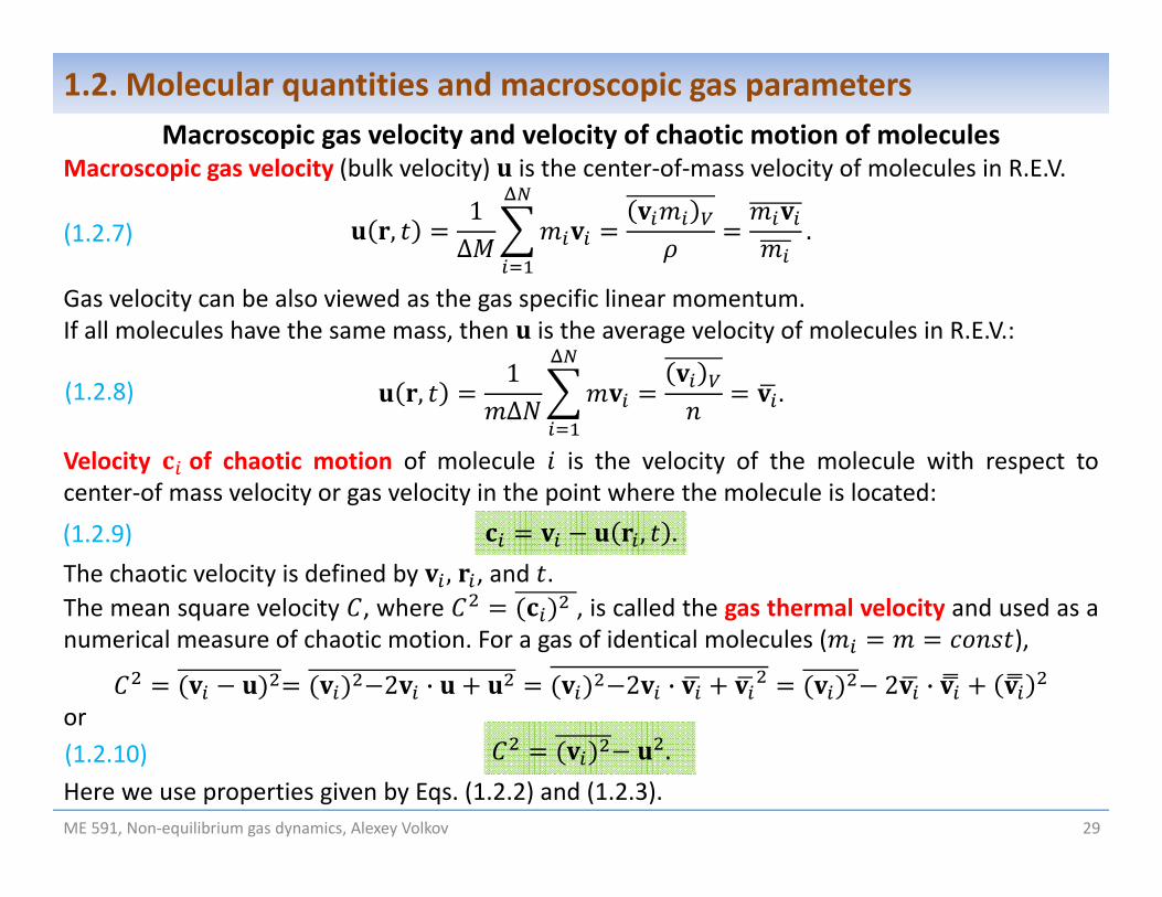
Macroscopic gas velocity (bulk velocity) is the center‐of‐mass velocity of molecules in R.E.V.
,1Δ .
Gas velocity can be also viewed as the gas specific linear momentum.If all molecules have the same mass, then is the average velocity of molecules in R.E.V.:
,1Δ .
Velocity of chaotic motion of molecule is the velocity of the molecule with respect tocenter‐of mass velocity or gas velocity in the point where the molecule is located:
, .The chaotic velocity is defined by , , and .The mean square velocity , where , is called the gas thermal velocity and used as anumerical measure of chaotic motion. For a gas of identical molecules ( ),
2 · 2 · 2 ·or
.Here we use properties given by Eqs. (1.2.2) and (1.2.3).
(1.2.7)
(1.2.8)
(1.2.9)
(1.2.10)

ME 591, Non‐equilibrium gas dynamics, Alexey Volkov 30
1.2. Molecular quantities and macroscopic gas parameters
(1.2.11)
(1.2.12)
(1.2.13)
(1.2.14)
Total and internal energiesThe total translational energy of a gas is the sum of kinetic energies of its molecules. Thespecific total translational energy and density of total translational energy are
,1Δ 2 , ,
1Δ 2 .
The internal or thermal energy of a monatomic gas is the kinetic energy of chaotic or thermalmotion of molecules. The specific internal energy is the internal energy of a unit mass anddensity of the internal energy is the internal energy of unit volume:
,1Δ 2 , ,
1Δ 2 .
In the case of molecules of the identical mass, :
,1Δ 2 2 2 2 , , 2 ,
and, if we use Eq. (1.2.10),
2 , 2 .
Thus, total specific energy is the sum of the specific internal energy and kinetic energy /2 ofthe gas macroscopic motion per unit mass.

ME 591, Non‐equilibrium gas dynamics, Alexey Volkov 31
1.2. Molecular quantities and macroscopic gas parametersRestrictions of the continuity hypothesis
The definition of macroparameters as volume‐averaged quantities has two major drawbacks:
Δ
Δ
∆
First, it can be applied only if the continuity hypothesis is satisfied.Let's imagine what can happen to Φ when we vary the size of averaging volume Δ . Two major cases are possible:
Case 1: R.V.E. exists
log Δ
Φ
Size of the volume is too small,number of molecules in ∆ is small,
fluctuations are significant
Size of the volume is too large compared to the flow length scale , gas state inside ∆ cannot be
considered as homogeneous
Range of R.E.V. sizes
Case 2: R.V.E. does not exist
log Δ
Φ
Transition from case 1 to case 2 occursif we gradually decrease the numberdensity of molecules (and increase ),i.e. if we consider more and morerarefied gas flows. Thus, the continuityhypothesis and our definition of fail inrarefied gas flows, which is the majorsubject of the kinetic theory.

ME 591, Non‐equilibrium gas dynamics, Alexey Volkov 32
1.2. Molecular quantities and macroscopic gas parametersSecond, the definition of Φ in the form of Eq. (1.2.1) can be used for real calculations only if weknow position vectors , velocities , and quantities Φ , , for all molecules in the gasflow.The definition of macroscopic gas parameters given in this section is well‐suited, e.g., foratomistic (molecular dynamics) simulations of matter (including gases), where positions andvelocities of all atoms are explicitly tracked by solving equation of motions for every atom in thesystem.In applications of the kinetic theory, the number of gas molecules is so huge that we cannottrace all of them. Later on, an alternative, kinetic (statistical) definition of macroscopic gasparameters will be given (Section 3.2). Eq. (1.3.1), however, will be in agreement with that newdefinition in the case when the continuity hypothesis is satisfied.

ME 591, Non‐equilibrium gas dynamics, Alexey Volkov 33
1.3. Gas laws Ideal gas equation of state Equation of state of calorically perfect gas Assumptions of elementary kinetic theory Kinetic foundation of the ideal gas equation of state Kinetic foundation of the equation of state of a calorically perfect gas Kinetic definition of gas temperature Brownian motion Equipartition of energy

Although initially Eq. (1.3.1) was established for particular processes likecompression of a fixed mass of a gas ( ) in a cylinder, it was found that thisequation holds for any process, where pressure and temperature vary within“reasonable” ranges. Therefore, this equation, often re‐written in the form
,is called the gas equation of state (EOS) or Clapeyron equation. A gas, whosethermodynamic parameters satisfy the Clapeyron equation, is called the ideal gas.ME 591, Non‐equilibrium gas dynamics, Alexey Volkov 34
1.3. Gas lawsIdeal gas equation of state
Physicists of XVIII century (Boyle, Charles, Gay‐Lussac, Avogadro, etc) experimentally establisheda number of gas laws, i.e. relationships between basic thermodynamic gas parameters such asmass , volume , number density , mass density , pressure , and absolutethermodynamic temperature .Many of these laws can be reduced to a single equation
where gas‐specific constant is called the gas constant, 8.3144598 J/mol/K is theuniversal gas constant, and is the molar mass. All parameters in the left‐hand side of Eq.(1.3.1) can be directly measured: / ( is the mass of the gas, is the occupied volume)with scale, with manometer, and with thermometer. Then the gas constant can bedetermined from experiment, [ ]=J/kg/K. The molar mass can be established without knowingmolecule mass and Avogadro constant in chemistry by measuring the relative masses ofspecies that participate in chemical reactions. Then one can find value of .
(1.3.1)
(1.3.2)

ME 591, Non‐equilibrium gas dynamics, Alexey Volkov 35
1.3. Gas lawsEquation of state of calorically perfect gas
Another series of experiments resulted in the relationship between the specific internal energyof the gas and its temperature
.
where the gas‐specific constant is called the gas specific heat at fixed volume, [ ]=J/kg/K.Absolute value of in Eq. (1.3.3) can not be directly measured, but the change of in, e.g.,adiabatic process ( 0) can be measured through the work performed by the gas using thefirst law of thermodynamics,
0,i.e. and
.
In the right‐hand side of the last equation, all quantities ( , , and ) can be directlymeasured experimentally. Similarly to Eq. (1.3.1), it was shown that Eq. (1.3.3) holds for anyprocess, where pressure and temperature vary within “reasonable” ranges. Therefore, thisequation, often re‐written in the form
,is called the gas equation of state. The gas, whose thermodynamic parameters satisfy Eq.(1.3.4), is called calorically perfect.
(1.3.3)
(1.3.4)

ME 591, Non‐equilibrium gas dynamics, Alexey Volkov 36
1.3. Gas lawsThe model of ideal and thermodynamically perfect gas is the model of gas, whosethermodynamic parameters satisfy two equations of state, (1.3.2) and (1.3.4). It is quite often,e.g., in gas dynamics, that the ideal and thermodynamically perfect gas is shortly called the idealgas. For example, the closed system of Euler equations is usually obtained in gas dynamicsspecifically for the gas satisfying both Eqs. (1.3.2) and (1.3.4).Equations of state are used in thermodynamics as empirical, i.e. established in experiments. Ourgoal is to show that these equations can be derived theoretically based on the assumptions ofthe molecular structure of a gas and chaotic motion of gas molecules. In addition, we willestablish a relationship between temperature and thermal velocity of individual molecules.
Assumptions of elementary kinetic theoryFor derivations, we will use only an elementary approach based on the following assumptions:1. We will consider a volume (vessel) occupied by a dilute
homogeneous gas, where there is no gradients ofmacroscopic parameters and macroscopic parametersare the same in any point of volume . For simplicity weconsider a vessel in the form a cube of size , containing molecules at number density / .
2. Every gas molecule is a “billiard” ball of diameterwithout internal structure. Position of a molecule can bedescribed by 3 Cartesian coordinates, i.e. a molecule has3 translational degrees of freedom.

3. Gas in volume is kept under fixed external conditions (e.g., fixed temperature of the vesselwall) for very long time. It is known from thermodynamics that in this case the gas reachesan equilibrium state, which does not change unless external conditions change (e.g., changeof the wall temperature or volume). We consider only the equilibrium state.
4. We will assume that the vessel is at rest, i.e. macroscopic gas velocity is zero, and, thus,chaotic velocity of every molecule is equal to its velocity in an inertial framework, .
5. We will not account for the real distribution of chaotic velocities of individual molecules. Wewill assume that that all molecules moves with the same averaged thermal velocity | |and /6 molecules at every time move toward any of 6 faces of cubic volume .
The theory that can be derived based on these assumptions is called elementary kinetic theory.Kinetic foundation of the ideal gas equation of state
ME 591, Non‐equilibrium gas dynamics, Alexey Volkov 37
1.3. Gas laws
Let be the force exerted on any face of vessel along normal to theface. Pressure is force exerted on a unit area, i.e. / / .Force appeares because individual molecules rebound from theface and exchange the momentum with the vessel. If gas and vesselare in equilibrium, then absolute value of average velocity of amolecule before and after the impact is the same. The only result ofinteraction is the change of velocity direction to the opposite one. Ifbefore the impact the molecule moves with momentum towardsa wall, then after the “reflection”, the molecule has momentum – .During the impact the molecule transfers momentum ∆ to the wall.
∆2
′

According to Newton’s second law of motion, force is the rate of change of momentum,∆ /∆ , and the pressure is the equal to ( )
∆∆ 3
Let’s compare Eq. (1.3.5) with the ideal gas EOS: These equations coincide if we assume that thethermodynamic temperature is defined by the average chaotic velocity of molecules as
3 or 2/2
3
ME 591, Non‐equilibrium gas dynamics, Alexey Volkov 38
1.3. Gas lawsNow let's consider the forces exerted on the face .In order to find let’s consider some interval of time ∆ anddetermine how many molecules ∆ interact with the faceduring this time. Such molecules must be located in the layer
′ ′ ′ ′ of thickness ∆ and volume ∆ ∆ andmove towards the wall, otherwise they will not reach the wallduring ∆ . Then ∆ 1/6 ∆ .The total momentum transferred to the wall during ∆ is equal to
∆ ∆ · ∆16 ∆ · 2
13 ∆
(1.3.5)
(1.3.6)

ME 591, Non‐equilibrium gas dynamics, Alexey Volkov 39
1.3. Gas laws
Kinetic foundation of the equation of state of a calorically perfect gasIf gas is dilute, then collisions between molecules are instant events and the number ofinteracting molecules an any particular time is negligibly small, so we can neglect contribution ofthe potential energy of interaction between gas molecules to the total gas energy. Then the totalinternal energy of gas in volume is the sum of kinetic energies of individual molecules /2.Then the specific internal energy (per unit mass) is equal to
/22 .
Eq. (1.3.7) coincides with the EOS of calorically perfect gas (1.3.4) if
2 or 3/2
3 .
Eqs. (1.3.6) and (1.3.8) result in32 ,
equation which is known from thermodynamics.
Thus, we see that both EOSs can be explained from the point of view of molecular structure ofgases if we assume that the gas temperature is a measure of averaged kinetic energy of chaoticmotion of individual gas molecules.
(1.3.8)
(1.3.7)

ME 591, Non‐equilibrium gas dynamics, Alexey Volkov 40
1.3. Gas laws
(1.3.11)
(1.3.9)
(1.3.10)
Kinetic definition of gas temperatureIn order to make the final step towards the kinetic definition of temperature let’s use therelationship between the gas constant and universal gas constant given by Eq. (1.3.1):/ . Then Eq. (1.3.6) reduces to
/2
/23 .
The new universal constant
1.38064852 × 10⁻²³ JK
is called the Boltzmann constant. With the Boltzmann constant, Eq. (1.3.9) can be re‐written as
213 2 ,
i.e. absolute thermodynamic temperature is such a measure of chaotic motion of molecules that/2 is equal to the average energy of chaotic motion of a single molecule per one degree of
freedom. This is the kinetic definition of temperature.
This definition is very general: In statistical physics, for any system in the equilibrium state,temperature is defined as such parameter that /2 is equal to the average energy of chaoticmotion of a single molecule per one degree of freedom.

ME 591, Non‐equilibrium gas dynamics, Alexey Volkov 41
1.3. Gas laws
(1.3.11)
(1.3.12)
(1.3.13)
With the Boltzmann constant, the gas constant can be defined as
,
and the EOSs of ideal and calorically perfect gas can be re‐written as follows
or ,
32
32 ,
or, for the internal gas energy per molecule ,32 .
Thus, the heat capacity of gas per unit molecule at constant volume is equal to 3/2 . Itmeans that /2 is equal to the heat capacity of the gas per one degree of freedom of gasmolecule.
The Boltzmann constant can be also considered as a scaling coefficient appeared in Eq. (1.3.11)because we used independent units to measure energy and temperature, that is why ] = J/K.
The Boltzmann constant establishes a proportionality between energy and temperature.

ME 591, Non‐equilibrium gas dynamics, Alexey Volkov 42
1.3. Gas laws
(1.3.14)
Equipartition of energy
In statistical physics, an equipartition theorem is formulated and proven. This theorem impliesthat, for any physical system in the equilibrium state, the energy is equally distributed betweenall degrees of freedom in this system, so that /2 is equal to the average energy of anydegree of freedom. Then, Eq. (1.3.11) for an equilibrium system with energy and degrees offreedom can be re‐written as follows:
2 .
If we consider a gas at equilibrium in a unit volume with number density , then 3 (everymolecule has 3 translational degrees of freedom) and /2 , so that Eq. (1.3.14)reduces to Eq. (1.3.11).The equipartition theorem highlights the fact that, in both thermodynamics and statisticalphysics, temperature is a quantity that characterizes, strictly speaking, only equilibrium states. Innon‐equilibrium states, the temperature can be introduced formally using Eqs. (1.3.11) or(1.3.14) as a measure of the internal energy, but different degrees of freedom have differentaverage energies, and these energies are not characterized by .Differences between energies of individual degrees of freedom, e.g., corresponding to thetranslational motion of molecules in , , and directions, can be used as measures of degreeof non‐equilibrium in gas flows (see Section 6.6).
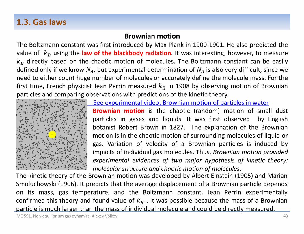
Brownian motionThe Boltzmann constant was first introduced by Max Plank in 1900‐1901. He also predicted thevalue of using the law of the blackbody radiation. It was interesting, however, to measure
directly based on the chaotic motion of molecules. The Boltzmann constant can be easilydefined only if we know , but experimental determination of is also very difficult, since weneed to either count huge number of molecules or accurately define the molecule mass. For thefirst time, French physicist Jean Perrin measured in 1908 by observing motion of Brownianparticles and comparing observations with predictions of the kinetic theory.
See experimental video: Brownian motion of particles in water
ME 591, Non‐equilibrium gas dynamics, Alexey Volkov 43
1.3. Gas laws
Brownian motion is the chaotic (random) motion of small dustparticles in gases and liquids. It was first observed by Englishbotanist Robert Brown in 1827. The explanation of the Brownianmotion is in the chaotic motion of surrounding molecules of liquid orgas. Variation of velocity of a Brownian particles is induced byimpacts of individual gas molecules. Thus, Brownian motion providedexperimental evidences of two major hypothesis of kinetic theory:molecular structure and chaotic motion of molecules.
The kinetic theory of the Brownian motion was developed by Albert Einstein (1905) and MarianSmoluchowski (1906). It predicts that the average displacement of a Brownian particle dependson its mass, gas temperature, and the Boltzmann constant. Jean Perrin experimentallyconfirmed this theory and found value of . It was possible because the mass of a Brownianparticle is much larger than the mass of individual molecule and could be directly measured.

ME 591, Non‐equilibrium gas dynamics, Alexey Volkov 44
1.4. Collision frequency. Free molecular, transitional, and continuum flow regimes
Homogeneous random distribution of molecules in space (in a volume) Probabilities of collisions with participation of various number of particles Collision frequency and mean free time Equilibrium and relaxation Knudsen number. Free molecular, transitional, and continuum flow regimes Local Knudsen number Local equilibrium. Summary on the length scales in dilute and dense gases

ME 591, Non‐equilibrium gas dynamics, Alexey Volkov 45
1.4. Collision frequency. Free molecular, transitional, and continuum flow regimes
The goal of the present section is to introduce major quantities characterizing the rate ofcollisions between molecules and to make conclusions on the effect of intermolecular collisionsunder various flow conditions. The first question is: Do we need to consider collectiveinteractions between molecules or it is sufficient to take into account only binary collisions? Toanswer this question we need to study random distributions of molecules in space.
Homogeneous random distribution of molecules in space (in a volume)
is called the probability to find our green molecule inside ∆ . Any probability of a randomevent is relative frequency of occurrence of this even among all possible outcomes (0 1).We say that molecules are distributed inside with equal probability (or homogeneously) if, forany molecule,
∆∆
.
Let's consider a volume filled with gas molecules at numberdensity / , choose a subvolume of size ∆ inside , andfix one (green) molecule. Since molecules move chaotically, wecan observe the green molecule sometimes inside ∆ ,sometimes outside. Let's assume that we determine position ofour molecule with respect to ∆ times ( ≫ 1) and foundthat it was inside ∆ times. Then the quantity
∆ lim→
∆∆
(1.4.1)

ME 591, Non‐equilibrium gas dynamics, Alexey Volkov 46
1.4. Collision frequency. Free molecular, transitional, and continuum flow regimes
Every time when we perform observations we can find more than one molecule inside ∆ . Let'scalculate the probability ∆ to find in ∆ (during one observation) molecules assumingwhat positions of individual molecules are independent from each other (i.e. presence orabsence of one molecule in ∆ does not affect presence or absence of any other moleculethere). For this purpose we can use the solution of statistical problem called the Bernoulli trial.In the Bernoulli trial (see Section 1.8), we perform independent measurements(determination of positions of particles with respect to ∆ ). Every measurement has only twooutcomes: Success (particle inside ∆ with probability ) or failure (particle outside ∆ withprobability 1 ). The probability of successes in a series of measurements is equal to
∆!
! ! P 1 .
Probabilities of collisions with participation of various number of particles
(1.4.2)
Binary collision is a process of interaction between two molecules.Triple collision is a process of interaction between three molecules.Let's compare probabilities of collisions with different number ofmolecules.If particles interact with each other, then they should be close toeach other, not farther than the characteristic length scale ofcollisions . Then a collision with participation of particlesoccurs if we can find particles in a sphere of radius and volume∆ 4π /3. Probability of such event is given by Eq. (1.4.2).
∆ 4π /3

ME 501, Non‐equilibrium gas dynamics, Alexey Volkov 47
1.4. Collision frequency. Free molecular, transitional, and continuum flow regimes
(1.4.3)
Now let's compare probabilities of collisions between 1 and molecules using Eq. (1.4.2):
1 1 1 1 1∆∆ .
This equation can be simplified in the case when ∆ ≪ and ≪ . Using additionally Eq.(1.4.1):
∆1
4 /31
4 /31 .
Thus, we see that
~ .
In the dilute gas, the density parameter is small, ≪ 1, and it is sufficient to account only forbinary collisions between molecules.In the dense gas, interactions between multiple particles (collective interactions) must be takeninto account.
In the kinetic theory of dilute gases, only binary collisions between molecules are accounted for.

ME 591, Non‐equilibrium gas dynamics, Alexey Volkov 48
1.4. Collision frequency. Free molecular, transitional, and continuum flow regimes
Collision frequency and mean free path
Mesh of cells
Collision frequency of a molecule is the meannumber of binary collisions which an individualmolecule participates in per unit time.In order to find , let’s first calculate the meannumber of collisions ∆ of a green molecule duringtime ∆ . During this time the molecule will make apath ∆ . Any other orange molecule canparticipate in the collision with the selectedmolecule only if the center of the orange moleculeis within the collisional cylinder of diameter andheight ∆ .Area of cross section of the collisionalcylinder is called the total collision cross section.The volume of collision cylinder is ∆ ∆ .
| |
∆
Then the number of collisions ∆ is equal to the average number of orange molecules in thecollision cylinder, ∆ ∆ ∆ , and the collision frequency for a molecule is equal to
∆∆ .
Collision density or collision frequency per unit volume is the mean number of binarycollisions in a unit volume per unit time. It can be easily found based on : Every molecule per
Collisioncylinder
(1.4.4)

ME 591, Non‐equilibrium gas dynamics, Alexey Volkov 49
1.4. Collision frequency. Free molecular, transitional, and continuum flow regimes
unit time participates in collisions and we totally have molecules in a unit volume. Then12
12 ,
where coefficient 1/2 appeared because two molecules participate in every binary collision.The mean free time of a molecule is the mean interval of time between two sequentialcollisions of a given molecule with other molecules:
1 1.
The mean free path of a molecule is the mean path a molecule travels between twosequential collisions with other molecules:
1.
The mean free path does not depend on thermal velocity . This quantitative result, however, isvalid only for billiard balls – molecules in the form of hard spheres of constant diameter .The obtained equations for , , , and are not accurate (sign “ ” is used) because we did notaccount for real distribution of chaotic velocities of individual molecules. The "accurate" theory,however, results in equations that are different only by some numerical coefficients. Forinstance, the "accurate" theory predicts that the mean free path of gas molecules in the form ofbilliard balls of diameter in the equilibrium state is equal to
12
.
(1.4.6)
(1.4.7)
(1.4.5)
More accurately, ∗ , where thecharacteristic velocity ∗ is not necessarilyequal to , but can be chosen based ondifferent considerations.

ME 591, Non‐equilibrium gas dynamics, Alexey Volkov 50
1.4. Collision frequency. Free molecular, transitional, and continuum flow regimes
Example: Basic collision properties in atmospheric air at standard conditions.
For N2, the major component of air, 3.7 Å and 46.5 · 10 kg (slide 9) and the gasconstant is equal to
1.38 · 1046.5 · 10 297
Jkg · K .
According to the kinetic definition of temperature, Eq. (1.3.11), at standard temperature of273.15 K:
3 3 493ms .
Number density at standard conditions is equal to the Loschmidt constant 2.6868 ·10 1/m (slide 13). Total collision cross section is equal to 43 · 10 m2. Then
Collision frequency of a molecule 5.7 · 10 1/s.
Collision density in a unit volume 7.7 · 10 1/s/m3.
Mean free time 0.18 · 10 s = 0.18 ns
Mean free path 0.086 · 10 m = 0.086 µm.
1. Thermal velocity is of theorder of sound speed,
, where is theisentropic index.2. The smaller , the largerthermal velocity at fixedtemperature. The highestthermal velocities at givenare specific for hydrogen andhelium.

ME 591, Non‐equilibrium gas dynamics, Alexey Volkov 51
1.4. Collision frequency. Free molecular, transitional, and continuum flow regimes
Equilibrium and relaxationThe major assumption (confirmed by observations) of thermodynamics is that every system (ofmolecules) under constant external conditions approaches with time an equilibrium state. Thesystem stays in equilibrium forever unless external conditions are changed.We cannot give a kinetic (statistical) definition of the equilibrium state right now, because it canbe done only based on the analysis of statistical distribution of chaotic velocities of individualmolecules in gases. We assume, however, that the kinetic theory must be in agreement withthermodynamics and any system of gas molecules in time should evolve towards theequilibrium state.The process of transition of any volume of gas from arbitrary initial non‐equilibrium state toequilibrium is called the relaxation. The characteristic time required to reach the equilibriumstate is called the relaxation time.
The major (and often the only) physical mechanism leading toequilibrium are collisions between gas molecules. The relaxationoccurs primarily due to intermolecular collisions.
The larger number of collisions between molecules, the fasterrelaxation and shorter relaxation time, so collisional propertieslike , , and can be used to characterize the rate of relaxation.
For molecules ‐ "billiard balls", equilibrium is established after afew collisions of every molecule, so that the relaxation time isusually assumed to be equal to the mean free time:
Example of extreme non‐equilibrium state:One energetic molecule
surrounded by molecules at rest
Such state cannot exist during longtime: After multiple collisionsbetween molecules, the initialenergy of the green molecule will bere‐distributed between all molecules

ME 591, Non‐equilibrium gas dynamics, Alexey Volkov 52
1.4. Collision frequency. Free molecular, transitional, and continuum flow regimes
Let's consider how collisions can affect properties of non‐homogeneous flows. Any non‐homogeneous flow has an intrinsic flow length scale(s) that characterizes the magnitude ofgradients of macroscopic gas parameters.
Knudsen number. Free molecular, transitional, and continuum flow regimesKnudsen number is the ratio of the characteristic mean free path ∗ to the flow length scale :
∗
For example, in aerodynamics problems, is usually chosen to be equal to the characteristic sizeof a body, and ∗ is defined by gas parameters in the undisturbed free stream around the body.
is measure of the importance of intermolecular collisions in the gas flow. Depending on thevalue of , three major regimes of the dilute gas flow can be introduced:
Continuum flow regime Transitional flow regime Free molecular flow regime ≪ 1 0.03 ~1 0.03 3 10 ≫ 1 3 10
L
Locally equilibrium flows (CGD) Non‐equilibrium flows (RGD)
(1.4.8)

ME 591, Non‐equilibrium gas dynamics, Alexey Volkov 53
1.4. Collision frequency. Free molecular, transitional, and continuum flow regimes
Continuum flow regime is a regime at ≪ 1, when every molecule is a subject of multiplecollisions inside the flow domain. Usually, in this case the continuity hypothesis is valid and,moreover, a system of molecules in any R.E.V. is in the state of local equilibrium, since thenumber of collisions is so large that it is sufficient for establishing equilibrium in R.E.V. This is theregime, when the gas flow can be satisfactory described by the continuum gas dynamics.Transitional flow regime is a regime at ~1, when every molecule participates only in a fewcollisions within the flow domain. The overall effect of collisions on the flow is non‐negligible,but the flow is strongly non‐equilibrium and continuum gas dynamics fails to describe suchflows. Flows in this regime can be described by only the kinetic theory. Most of simulations offlows in the transitional regime is performed by the Direct Simulation Monte Carlo method.Free molecular or collisionless flow regime is the regime at ≫ 1, when collisions are soinfrequent that can be completely neglected. In this case the flow is primarily governed by thelaws of interaction of individual molecules with walls or interfacial boundaries. Such flows arestrongly non‐equilibrium and computed based on the kinetic theory, but many free molecularflow problems admit theoretical solutions and do not require numerical simulations. The ranges of for every regime shown in the previous slide are approximate: They depend
on problem under consideration and on the adopted choice of ∗ and in the definitionof Kn. Example: Flow over a sphere. Traditionally is based on the sphere radius ( ),but we can also define based on the sphere diameter ( 2 ).
There are flows that cannot be characterized by a single value of common for the wholeflow. Such flows can include local zones corresponding to different flow regimes.

ME 591, Non‐equilibrium gas dynamics, Alexey Volkov 54
1.4. Collision frequency. Free molecular, transitional, and continuum flow regimes
Soot nanocluster Atmosphere of Io
3640 km
The degree of flow rarefaction depends not only on the properties of the gas itself (molecule size, numberdensity, etc.), but it is also essentially determined by the flow length scale. The degree of rarefaction is theflow property, not the gas property!In the same gas, e.g., in air at standard conditions, one flow (on the scale of ~1 m, ~10 ) can becontinuum, while other (on the scale of ~1 µm, ~0.1) can be transitional or even free molecular.
These are both
transitional flow !

ME 591, Non‐equilibrium gas dynamics, Alexey Volkov 55
1.4. Collision frequency. Free molecular, transitional, and continuum flow regimes
Local Knudsen numberOne of the major example of flows that could not be characterized by a single Knudsen numberis the flow in a free jet expanding into vacuum or low‐pressure background gas. Inside thenozzle or around it, the flow can be continuum, but then the gas density gradually drops to zero,so the jet flow field can include the zones of continuum, transitional, and free molecular flow.
A criterion that allows one to distinguishbetween zoned with different flow regimes iscalled a continuum breakdown criterion.There are a lot of empirical breakdowncriterions suggested, with the most popularbased on the local Knudsen number
,,, ,
where , is the local mean free path(defined in the point r of the flow field) and
, is the local flow length scale that isoften based on the characteristic length scaleof the density variation (density gradient ):
, .
Free molecular
Transitional
Continuum.
normalized density contours /

ME 591, Non‐equilibrium gas dynamics, Alexey Volkov 56
1.4. Collision frequency. Free molecular, transitional, and continuum flow regimes
Strong density drop occurs not only in the jet, but also in the diverging part of the Laval nozzle.
Density drops in more than order of
magnitude

ME 591, Non‐equilibrium gas dynamics, Alexey Volkov 57
1.4. Collision frequency. Free molecular, transitional, and continuum flow regimesRelaxation length. Local equilibrium. "Extended" continuity hypothesis
if we consider a small volume of size , then every molecule travels through this volume duringthe relaxation time . And, thus, the total number of collisions in such volume is enough to turnthe system of gas molecules in this volume into the local equilibrium state. Therefore the meanfree path can be considered as the relaxation length, i.e. characteristic length scale of volumesin the gas flow, where the local equilibrium can be established due to collisions betweenmolecules. Note, the Eq. (1.4.7) can be re‐written as follows
1 1~ ,
where is the density parameter. Then let's estimate the number of molecules in :1.
Assume that we have a continuum gas flow ( ≪ ) of a dilute gas ( ≪ 1, practically 10 ).Then the choice of a R.E.V. size equal to the relaxation length satisfies all requirements to R.E.V:1. R.E.V. contains many particles (more than 106 according to Eq. (1.4.8)), so that the definition
of macroscopic parameters as volume‐averaged molecular quantities makes sense: Itproduces values that do not fluctuate because of chaotic motion of molecules.
2. R.E.V. is small compared to the flow length scale, providing homogeneous distribution ofmolecules in R.E.V.
3. Moreover, since the R.E.V. size is in the order of relaxation length, in every R.E.V. gasmolecules are in local equilibrium, so that we can use multiple relationships established,e.g., in thermodynamics, for equilibrium systems.
(1.4.9)

Thus, we see that in the continuum flow regime of a dilute gas an "extended" continuityhypothesis, which includes requirements 1, 2, and 3, is valid. Local equilibrium of gas flows inthe continuum flow regime is intensively used in gas dynamics, where the conservation laws(mass, momentum, and energy equations) are supplied with multiple closure equations(equations of state, Newton's law for viscous stresses, Fourier's law for heat flux, etc.) that arenecessary to obtained a closed system of equations (a system where the number of unknowns isequal to the number of equations), but valid only in conditions of local equilibrium.
Summary on the length scales in dilute and dense gasesWe introduced four linear (and time) scales of processes in gases: collision length scale , meandistance between molecules , relaxation length – mean free path , and flow length scale .Depending on the nature of the gas (dense/dilute) and flow regime (continuum/non‐continuum) we have the following relationships between these scalesIn a dense gas (density parameter ~1):
~ ~ ~ ~ ~
In a dilute gas (density parameter ≪ 1):
~ ≪ ~ ≪ ~
In continuum flows of a dilute gas ( ≪ 1, ≪ ):
~ ≪ ~ ≪ ~ ~ . . . ≪
ME 591, Non‐equilibrium gas dynamics, Alexey Volkov 58
1.4. Collision frequency. Free molecular, transitional, and continuum flow regimes
Gas dynamics,
CFD
Rarefied gas dynamics, DSMC

ME 591, Non‐equilibrium gas dynamics, Alexey Volkov 59
1.5. Transfer of molecular quantities Processes of transfer of physical quantities Fluxes and flux densities of physical quantities Convective and collisional transfer of molecular quantities

ME 591, Non‐equilibrium gas dynamics, Alexey Volkov 60
1.5. Transfer of molecular quantitiesProcesses of transfer of physical quantities
Let’s consider some conservative physical quantity Φ, i.e. aphysical quantity which is conserved in a closed physicalsystem. Examples of conservative quantities: Number ofparticles, mass, linear momentum, angular momentum,energy, etc.
Since such quantity cannot “appear” or “disappear’, a non‐homogeneous distribution of such physical quantity in spacecan evolve only by means of re‐distribution of this physicalquantity in space. Physical processes of re‐distribution ofconservative physical quantities are called the transferprocesses. From the point of view of molecular structure ofmatter, all transfer process are related to the motion andinteraction of individual particles (electrons, atoms,molecules) or propagation of electromagnetic waves.
Example: Diffusion is the mixing of two matters that arebrought in contact with each other. Diffusion is the particlenumber transfer process. Non‐reversible mixing occurs as aresult of chaotic motion of molecules. Diffusion happens ingases (fastest), liquids, and solids (slowest).
Time
ΦΦ
Transfer of ΔΦ during Δ
Φ ΔΦΦ ΔΦ

ME 591, Non‐equilibrium gas dynamics, Alexey Volkov 61
1.5. Transfer of molecular quantities
Fluxes and flux densities of molecular quantitiesIn continuum mechanics we systematically use such macroscopic parameters as fluxes and fluxdensities, e.g., heat flux, in order to describe transfer process of various molecular quantities.For a given surface and direction specified by the unit normal vector to the surface, fluxof physical quantity Φ is the amount of this quantity which is transferred through surface
in the direction of per unit time, [ ]=[Φ]/s. For example, energy flux has unit of J/s.The flux density of physical quantity Φ is such vector quantity that the flux through anysurface of infinitesimal area with unit normal is equal to · , so the fluxdensity can be considered as the flux of Φ per unit area, [ ]=[Φ]/s/m2. For example, energydensity flux has unit of J/s/m2.
Flux and flux density can be both positive and negative. Negative value ofthe flux means that the corresponding physical quantity is preferentiallytransferred through surface in the direction opposite to .
Surface
· , flux through infinitesimal area ;
Flux through the whole surface is equal to
· . This is the surface integral (see calculus)

ME 591, Non‐equilibrium gas dynamics, Alexey Volkov 62
1.5. Transfer of molecular quantities
Convective and collisional transfer of molecular quantitiesFrom the point of view of molecular structure of a gas, transport of any physical quantitythrough any surface is a result of motion and interaction of individual gas molecules.
Two mechanisms of transfer of molecular quantities:Free motion of molecules through surface : If during time ∆ a molecule (molecule 1) movesfrom volume to volume through surface or vise versa (molecule 2) then amount ofquantity Φ in decreases in and increases in . This mechanisms of transfer of molecularquantities is called convective. Its contribution to the momentum flux is called kinetic.Interaction of molecules at different sides of surface : Total quantity of Φ in can changebecause some molecules in this volume (molecule 3) interact by forces with molecules(molecule 4) in . This interaction will result in the redistribution Φ between and induring time ∆ even if molecules do not cross the surface . This mechanisms of transfer ofmolecular quantities is called collisional. Its contribution to the momentum flux is called virial.
Time Surface
1
2
3 4
Time Δ
12
3 4
Interaction between molecules 3 and 4
Free motion ofmolecules 1 and 2through surface

Value of Δ can be estimated like value of ∆ in slide 37
Δ∆6 .
Molecules contribute to collisional transfer if they are located atdifferent sides of and participate in collisions. Then Δ canbe estimated as the total number of collisions occurring in thelayer of thickness 2 around surface :
Δ 2 Δ Δ Δ .Then
ΔΔ 6 ~
In a dilute gas, the density parameter is small, ≪ 1, andcollisional transfer is small compared to the convective one. Inthe kinetic theory of dilute gases, collisional transfer is neglected.
ME 591, Non‐equilibrium gas dynamics, Alexey Volkov 63
1.5. Transfer of molecular quantitiesLet’s compare the relative contributions of convective and collisional transfer of molecularquantities in gas flows.The rates of change of a conservative quantity due to convective and collisional transfer dependon the number of molecules that participate in every type of transfer processes. Let’s considersome planar surface of area and estimate the number of molecules that participate inconvective, Δ , and collisional transfer, Δ , through during time Δ .
Δ

ME 591, Non‐equilibrium gas dynamics, Alexey Volkov 64
1.6. Transfer equation Simple transfer equation Homogenization of macroscopic parameters as a result of chaotic motion

ME 591, Non‐equilibrium gas dynamics, Alexey Volkov 65
1.6. Transfer equationSimple transfer equation
Let’s obtain a macroscopic transfer equation that describes transfer of some molecular quantityΦ due to chaotic motion of molecules under conditions when the "extended" continuityhypothesis is valid.
ΔΦ ,
Φ Δ
Φ Δ
Ψ ,
Δ
Let’s assume that Convective transfer is the only reason for change of
macroscopic gas parameters (no external forces, etc.) Transfer occurs in the direction of axis and divide the
flow into R.E.V. in the form of cubic cells of size Δ .Φ , is the density ofΦ in the cell with center at .Ψ , is the density of flux of Φ that is transferred fromcell into neighbor cells with centers Δ and Δ .We assume that in every R.E.V. (every cell) gas is in localequilibrium, so that Δ . The total quantity of Φtransferred from cell to any neighbor cell during Δ isthen equal to
ΔΦ Ψ , Δ16 Δ Φ
16 Δ Φ
Ψ ,16 Φ .
Cell
Cell Δ
and

ME 591, Non‐equilibrium gas dynamics, Alexey Volkov 66
1.6. Transfer equationThen we can write an equation of balance of total amount ofΦin cell during time Δ :
Δ Φ , Δ Δ Φ , Ψ Δ , Ψ Δ , 2Ψ , Δ Δ .
If we divide the equation by Δ Δ , then we get
Φ , Δ Φ ,
ΔΨ , Ψ Δ , Ψ Δ , Ψ ,
ΔHere
Δ2 , Ψ , Ψ Δ , 6
Φ Δ ΦΔ
is the density of flux of Φ between cells and Δ . Then
Φ , Δ Φ ,Δ
Δ /2, Δ /2,Δ .
Finally, let's consider Eqs. (1.6.1) and (1.6.2) in the limit when Δ → 0 and Δ → 0
Φ, 6 ,
Φor
Φ Φ.
0 if transfer of Φ occurs in the positive direction of
axis .
(1.6.1)
(1.6.3)
(1.6.4)
(1.6.2)

ME 591, Non‐equilibrium gas dynamics, Alexey Volkov 67
1.6. Transfer equationEq. (1.6.3) establishes a linear relationship between the flux density of molecular quantity andgradient of corresponding macroscopic parameter. The sign “‐” in Eq. (1.6.3) means that thetransport of molecular quantity preferentially occurs in the direction opposite to the direction ofthe gradient, i.e. from regions where density of Φ is large to regions where density of Φ is small.Coefficient of proportionally in Eq. (1.6.3) is called the transfer (transport) coefficient. isnot a constant, since depends on ( ~ ), and depends on and, in general, on . Thus,the larger , the larger and the rate of the transfer process.Equation (1.6.4) is the simple transfer equation. It can be applied to study transfer of variousmolecular quantities.
The question is: Where did we use in derivation of Eq. (1.6.4) the "extended" continuityhypothesis?One can notice that me made a “trick” in derivation of Eq. (1.6.3) from Eq. (1.6.2). Namely, wefirst assumed Δ , but then considered the case when Δ → 0 at fixed :
6Φ Δ Φ
Δ → 6Φ
This "trick" is in based on the assumption that the "extended" continuity hypothesis is valid. Wecannot arbitrary change since it is given by physical properties of our flow, but, since ≪ ,we can consider Δ as an infinitely small size compared with the flow length scale .

ME 591, Non‐equilibrium gas dynamics, Alexey Volkov 68
1.6. Transfer equation
Let’s solve a boundary value problem for Eq. (1.6.4)assuming that
Φ Φ
with the initial distribution of Φ in the form of a stepfunction
At 0:Φ , 0 , 0;, 0.
Solution takes the form (can be checked by substitution)
Φ , 2 2 erf2
,
where erf is the error function:
erf2
.
Homogenization of macroscopic parameters as a result of chaotic motion
Φ
Chaotic motion results in non‐reversible homogenization of initial non‐homogeneous distributionof macroscopic parameter . As a result of chaotic motion, quantity is transferred fromlayers with larger to layers with smaller . The rate of this process is defined by .
Limit homogeneous distribution at → ∞
(1.6.5)0.1 ∗ ∗ 3 ∗9 ∗
∗

Note that solution in the form of Eq. (1.6.5)depends not on individual values of and ,but on the variable / . It meansthat at any time ∗, the characteristic linearscale of the domain ∗ affected by thetransfer of molecular quantity is equal to
∗ ∗.
This equation establishes a simple, butuniversal relationship between time , ∗, andlength , ∗, scales of the transfer process.This equation can be used as follows: If weknow that the transfer process through someboundary occurs during time ∗ , then thedomain around this boundary, wheremacroscopic parameters are affected by thisprocess, has the characteristic size ∗ given byEq. (1.6.6).
ME 591, Non‐equilibrium gas dynamics, Alexey Volkov 69
1.6. Transfer equation
(1.6.6)
∗
Φ
0.1 ∗ ∗ 3 ∗9 ∗
Limit homogeneous distribution at → ∞
∗1

ME 591, Non‐equilibrium gas dynamics, Alexey Volkov 70
1.7. Diffusion, viscous drag, and heat conduction Diffusion Viscous drag Heat conduction

ME 591, Non‐equilibrium gas dynamics, Alexey Volkov 71
1.7. Diffusion, viscous drag, and heat conductionDiffusion
Diffusion in gases is the physical process of redistribution of number of molecules by means ofpreferential motion of molecules from regions where molecules more abundant to regionswhere they are less abundant due to chaotic motion of molecules. In the important case ofbinary diffusion, two different gases are mixing with each other. Binary diffusion cannot beconsidered based on the simple transfer equation, because it was derived for a gas composed ofidentical molecules. Let’s apply the transfer equation
Φ,
Φ, 6
in order to describe self‐diffusion, e.g. homogenization of distribution of number density in agas of identical molecules. We consider Φ 1, Φ 1, and assume that there is a non‐homogeneous distribution of number density Φ , along axis . Then the number fluxdensity in direction is given by the equation
,where
63
61 1
~
is called the self‐diffusivity or self‐diffusion coefficient.
,Layer where
molecules are more abundant
Layer where molecules are less
abundant
Direction of preferential transfer of
molecules due to their chaotic
motion
(1.7.1)
(1.7.2)

ME 591, Non‐equilibrium gas dynamics, Alexey Volkov 72
1.7. Diffusion, viscous drag, and heat conductionThe transfer equation takes the form
or
and is called the diffusion equation. The linear relationship between the diffusion flux densityand gradient of number density of molecules given by Eq. (1.7.1) is called Fick's law of diffusion.It was first established experimentally. We showed that this experimental law in gases isexplained by the chaotic motion of molecules.Eq. (1.7.2) is not accurate, but predicts correct functional dependence of on and : The“accurate" kinetic theory predicts that for gas composed of hard sphere (HS) molecules
38
1 1.
The experiments show that the (self‐)diffusion coefficient varies as a function of and as
~ ,where exponent can be different from ½. The “accurate” kinetic theory shows that thedependence of on is determined by the model of interaction between gas molecules.Models that are more sophisticated that the HS model can accurately predict Eq. (1.7.5).Note: In the kinetic theory, self‐diffusion has a limited importance (contrary to diffusion ofdifferent species) and usually considered as a limit case of binary diffusion of two gases withsimilar and .
(1.7.3)
(1.7.4)
(1.7.5)

is called the shear stress and
612 3
~
is called the (dynamic) (shear) viscosity (coefficient). Transfer equation takes the form
or
ME 591, Non‐equilibrium gas dynamics, Alexey Volkov 73
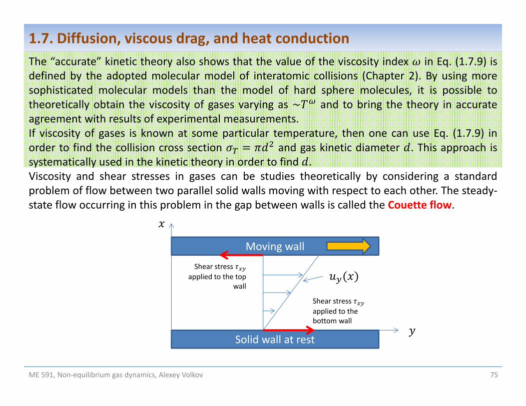
1.7. Diffusion, viscous drag, and heat conductionViscous drag
Viscosity of a fluid (informally) is ability of fluid to resist the shear load. Viscous drag in gases isthe physical process of redistribution of angular momentum in the direction perpendicular tothe flow velocity from layers with higher gas velocity to layers with smaller gas velocity. Let’sapply the transfer equation
Φ,
Φ, 6
in order to describe viscous drag. We consider Φ , then Φ and Φ Φ, and assume that there is a non‐homogeneous distribution of , along axis , while
. Then the flux density of ‐component of angular momentum through a surfacenormal to axis is given by the equation
(1.7.6)
(1.7.7)
(1.7.8)
Faster moving layer
Slower moving layer
Direction of preferential transfer of
momentum due to chaotic
motion of molecules
,
Shear force thatdecelerates top layer
Shear force thataccelerates bottom layer

ME 501, Non‐equilibrium gas dynamics, Alexey Volkov 74
1.7. Diffusion, viscous drag, and heat conductionand is called the viscous drag equation. The shear stress has unit of kg∙(m/s)/s/m2 = N/m2 = Pa since this is a force (flux of linearmomentum) per unit area. The quantity characterizes the tangential or shear force appliedto a unit area on a surface with normal along axis and acting along axis . The linearrelationship between the shear stress and gradient of macroscopic velocity, Eq. (1.7.6), is knownas Newton's law of viscosity. It was first established experimentally. We showed that thisexperimental law in gases is explained by the chaotic motion of molecules.Eq. (1.7.6) establishes two important facts about the viscosity coefficient:1. Viscosity of dilute gases does not depend on number density. This fact is in accurate
agreement with experiments.2. Viscosity is proportional to / . Experimentally, it is know that the dependence of viscosity
on temperature in some limited range of temperature can be well‐approximated by thepower law
,
where the viscosity index varies between 1/2 and 1 with values 1/2 specific for higher and1 for lower . The “accurate” kinetic theory predicts that value 1/2 is specific only for hardsphere molecules with the accurate value of viscosity equal to
516 .
(1.7.9)
(1.7.10)
ME 591, Non‐equilibrium gas dynamics, Alexey Volkov 75
1.7. Diffusion, viscous drag, and heat conductionThe “accurate” kinetic theory also shows that the value of the viscosity index in Eq. (1.7.9) isdefined by the adopted molecular model of interatomic collisions (Chapter 2). By using moresophisticated molecular models than the model of hard sphere molecules, it is possible totheoretically obtain the viscosity of gases varying as ~ and to bring the theory in accurateagreement with results of experimental measurements.If viscosity of gases is known at some particular temperature, then one can use Eq. (1.7.9) inorder to find the collision cross section and gas kinetic diameter . This approach issystematically used in the kinetic theory in order to find .Viscosity and shear stresses in gases can be studies theoretically by considering a standardproblem of flow between two parallel solid walls moving with respect to each other. The steady‐state flow occurring in this problem in the gap between walls is called the Couette flow.
Solid wall at rest
Moving wall
Shear stress applied to the top
wall
Shear stress applied to the bottom wall

,
is called the heat flux density and
632 ~
is called the thermal conductivity (coefficient). The transfer equation takes the form
or .
ME 591, Non‐equilibrium gas dynamics, Alexey Volkov 76
1.7. Diffusion, viscous drag, and heat conductionHeat conduction
Heat conduction or heat transfer in gases is the physical process of redistribution of internalenergy from hotter to colder regions due to chaotic motion of molecules. Let’s apply thetransfer equation
Φ,
Φ, 6
in order to describe heat conduction. We consider Φ /2 /2 (no bulk velocity),then Φ /2 3/2 (see Eq. (1.3.11)) and Φ Φ 3/2 , andassume that there is a non‐homogeneous distribution of temperature , along axis , whilethere is only minor inhomogeneity of , so (see the comment on slide 78). Then theenergy flux density in direction, , given by the equation
32
(1.7.11)
(1.7.12)
(1.7.13)
Hotter layer
Colder layer
Direction of preferential transfer of energy due to chaotic motion of molecules
,

and is called the heat conduction equation. The heat flux density has unit of J/s/m2 = W/s . The linear relationship between the heat fluxdensity and gradient of temperature, Eq. (1.7.11) is known as Fourier’s law of heat conduction.It was first established experimentally. We showed that this experimental law in gases isexplained by the chaotic motion of molecules.Eq. (1.7.12) establishes two important facts that are in agreement with experiments:1. Thermal conductivity of gases does not depend on number density2. Thermal conductivity is proportional to viscosity i.e. varies with temperature as the viscosity
does. Experiments show that the Prandl number
,
where is the specific heat at constant pressure ( 5/2 for a monatomic gas), in a“reasonable” range of is independent of temperature and its value for many gases is about2/3. Then varies with temperature as in Eq. (1.7.9), i.e. / .Our elementary theory fails to predict the accurate value of Pr. The "accurate" kinetic theoryshows that for any monatomic gas 2/3, and thus
32 .
In particular, for hard sphere molecules (use Eq. (1.7.10)),
7564 .
ME 591, Non‐equilibrium gas dynamics, Alexey Volkov 77
1.7. Diffusion, viscous drag, and heat conduction
(1.7.14)
(1.7.15)
(1.7.16)

ME 591, Non‐equilibrium gas dynamics, Alexey Volkov 78
1.7. Diffusion, viscous drag, and heat conductionThe “standard” test problem for heatconduction is the steady‐state heatconduction in a gas between twoparallel planes at fixed temperaturesand .This problem allows one to illustrate theprincipal difference between transferprocesses in continuum and freemolecular flow regime.In free molecular flow, the temperatureis constant because the flow is formedby two homogeneous streams ofmolecules that do not interact with eachother: Stream of molecules movingfrom bottom to top and equilibratedwith the bottom wall at temperatureand stream of molecules moving fromthe top to the bottom and equilibratedwith the top wall at . Withoutcollisions, energy between these twostreams is not equilibrated.
/ ≪ 1
Distribution given by condition
/ ≫ 1
Constant
Temperature jump: Difference between surface temperature and gas temperature
In heat conduction problem,the gas density is not aconstant, since for themechanical equilibrium (nobulk velocity andmacroscopic flow) pressureshould be constant acrossdomain, i.e. is given bythe condition
.

ME 591, Non‐equilibrium gas dynamics, Alexey Volkov 79
1.8. Appendix: Probability and Bernoulli trial Random outcome and event. Sure and impossible events Union and intersection of events. Compliment, and mutually exclusive events Statistical definition of probability of a random event Calculation of probabilities Dependent and independent random events. Conditional probability Bernoulli trial

ME 591, Non‐equilibrium gas dynamics, Alexey Volkov 80
1.8. Appendix: Probability and Bernoulli trialLet's assume that we consider some stochastic system, process, or phenomenon that can berepeated many times in identical conditions. The elementary event or outcome is the random output of any individual observation or
measurement. The event is an arbitrary set of possible outcomes. The sure event Ω is the event that includes all possible outcomes. The impossible event ∅ is an event that has no chance to occurring. It includes neither of the
outcomes.Example: Playing dieStochastic process (experiment): Rolling the die and registeringthe number of dots on the top face.Outcome: The number of dots on the top face afterindividual rolling of the die.Possible outcomes:
1 , 2 , ..., 6Examples of events: 1or 5 1and 4 1or 5or 6
Ω 1or 2or … or 5or 6∅ 1or 6

ME 591, Non‐equilibrium gas dynamics, Alexey Volkov 81
1.8. Appendix: Probability and Bernoulli trial Every elementary event is an element (point) of Ω. Every event is a subset of points of Ω. It is illustrative to use Venn diagrams to demonstrate the relationship between the sure
event, elementary events, and various other events.
A union ∪ of two events and is the event which happens if or happen.
Sure event Ω, full set, full area
Event = subset, subareaElementary event,outcome, point
∪
Example: Playing die
1or 2
2or 6
5
∪ 1or 2or 6
∪ 1or 2or 5

ME 349, Engineering Analysis, Alexey Volkov 82
1.8. Appendix: Probability and Bernoulli trial An intersection ∩ of two events and is the event which happens if and happen
simultaneously.
Event ′ is called compliment to event if ∪ ′ Ω and ∩ ′ ∅ .
Events and are calledmutually exclusive if ∩ ∅.
Example: Playing die
1or 2
2or 6
5
∩ 2
∩ ∅
′ 3or 4or 6or 6
∩
′
and are mutually exclusive ′ is compliment to

Simple rules for random events
∪ ∪ , ∩ ∩
∪ ∪ ∪ ∪
∩ ∪ ∩ ∪ ∩
∪ ∪ , ∩ ′ ′ ∩ ′
∪ , ∩
∪ Ω Ω, ∩ Ω
∪ ∅ , ∩ ∅ ∅
Probability of a random event
Probability of a random event is a numerical measure of our degree of confidence that theevent happen during a single outcome (experiment, measurement) of the consideredstochastic system (process, phenomenon).
There are at least four different definitions of probability. We will use only an intuitively clear,statistical definition of probability.
ME 591, Non‐equilibrium gas dynamics, Alexey Volkov 83
1.8. Appendix: Probability and Bernoulli trial
All these rules can be easily proved with Venn diagrams.

Let's assume that we repeat our observation (experiment) times ( ≫ 1) independently fromeach other, but in identical conditions and random event happened times among .
Probability of event is the relative frequency of this event among others, calculated inthe limit → ∞:
lim→
Simple properties of probability drawn from the fact that for any random event:
0 1. ∅ 0, because ∅ 0. Ω 1, because Ω . If ⊂ , then , because . If and are mutually exclusive events ( ∩ ∅), the probability of a union is equal to
the sum of probabilities (summation rule):∪
because for mutually excusive events ∪ . Since ∪ Ω, ∩ ∅, then Ω and 1 .
ME 591, Non‐equilibrium gas dynamics, Alexey Volkov 84
1.8. Appendix: Probability and Bernoulli trial
(1.8.1)
(1.8.2)

Independent events and conditional probability
The conditional probability | is the probability of event calculated under the conditionthat event occurs. This probability accounts for the fact that occurrence of event changesprobability of event :
or∩
It is reasonably to call two random events and independent if the happening of one ofthese event does not affect the probability of occurrence of another, i.e. if | and
| .
In order to draw Eq. (1.8.3), has to occur, i.e. 0.
Then for independent events and we have themultiplication rule:
∩ ⟺ and are independent
The main purpose of the probability theory is to formulate rules that allow us to calculateprobabilities of complex events based on known probabilities of simple events.
ME 591, Non‐equilibrium gas dynamics, Alexey Volkov 85
1.8. Appendix: Probability and Bernoulli trial
| lim→
∩lim→
∩ //
∩(1.8.3)
(1.8.4)
(1.8.5)
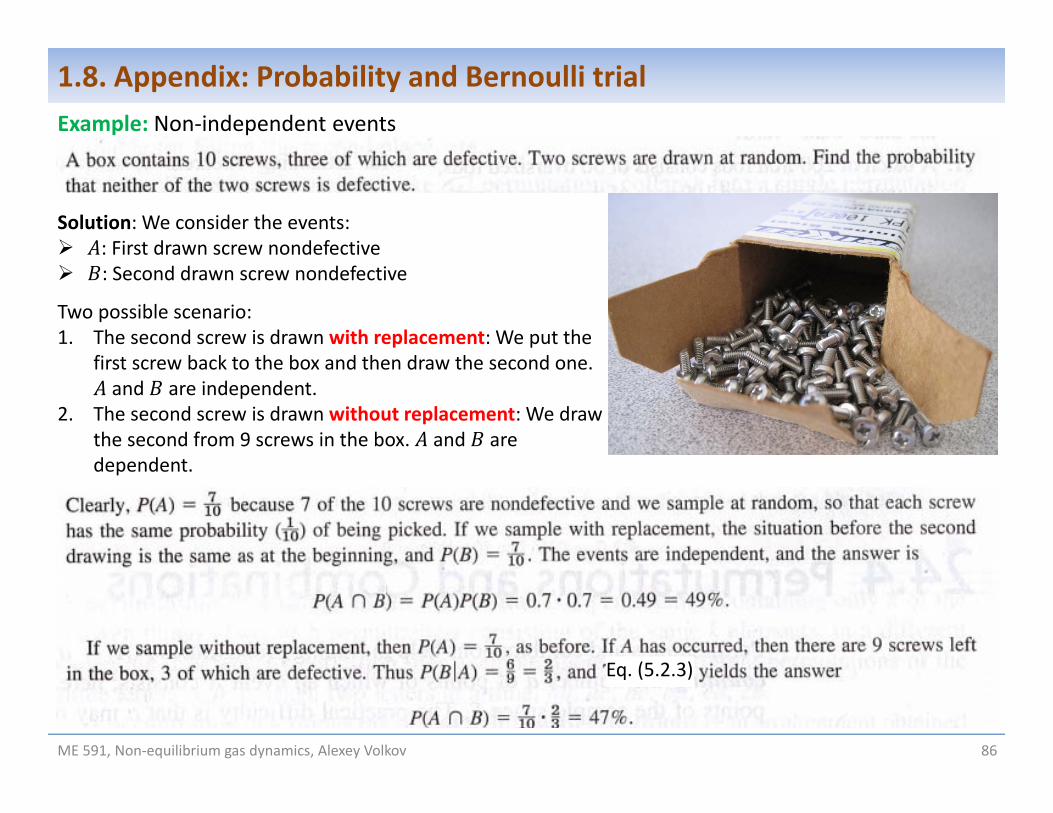
ME 591, Non‐equilibrium gas dynamics, Alexey Volkov 86
1.8. Appendix: Probability and Bernoulli trialExample: Non‐independent events
Eq. (5.2.3)
Solution: We consider the events: : First drawn screw nondefective : Second drawn screw nondefective
Two possible scenario:1. The second screw is drawn with replacement: We put the
first screw back to the box and then draw the second one. and are independent.
2. The second screw is drawn without replacement: We draw the second from 9 screws in the box. and are dependent.

The previous example falls into general category of problems known as Bernoulli trial that canbe solved with or without replacement. We will consider the Bernoulli trial with replacement.
Bernoulli trial with replacementA Bernoulli trial (or binomial trial) is a random experiment or test with exactly two possibleoutcomes, "success" and "failure", in which the known probability of success is the same everytime the experiment is conducted.Two elementary events (outcomes): , . The sure event Ω , }Two known probabilities of every outcome: , 1 .Example 1: Rolling die. 6 , 1 5 , 1/6, 5/6.Example 2: A pile of grey andM red balls. We pick upat random one ball from the pile, determine its color andreturn the ball to the pile.
Ballisgray, / .Ballisred, / 1 .
This is the Bernoulli trial with replacement, since everytest is performed in the same conditions (We determinecolor and return ball to the pile).
ME 591, Non‐equilibrium gas dynamics, Alexey Volkov 87
1.8. Appendix: Probability and Bernoulli trial

ME 591, Non‐equilibrium gas dynamics, Alexey Volkov 88
1.8. Appendix: Probability and Bernoulli trialAssume that we performed the test times. The major question in the Bernoulli trial is:What is the probability of choosing (0 ) grey balls after test?First let's consider an example when 3 and calculate 1 .In three sequential tests we can chose 1 grey ball as follows
Since events 1, 2, and 3 are mutually excusive, one can use the summation rule:1 1 ∪ 2 ∪ 3 1 2 3 3 1
In the general case (arbitrary and ) one can obtain:
1
where the integer value denoted as is called the binomial coefficient and is equal to thenumber of different events with grey balls drawn in tests
!! !
In our example ( 3 and 1), 31!
! !· ·· ·
3.
Event Test 1 Test 2 Test 3 Probability (all tests in a sequence are independent)
Event 1 Grey Red Red 1 1Event 2 Red Grey Red 2 1Event 3 Red Red Grey 3 1
(1.8.6)


