Chapter 1: A Framework for Agricultural Policy Analysis · Sjaiful Bhari June 2003 . ... Profits,...

COMPUTER TUTORIAL

FOR

POLICY ANALYSIS MATRIX (PAM) IN INDONESIAN AGRICULTURE

Carl H. Gotsch Scott R. Pearson

Sjaiful Bhari

June 2003

TABLE OF CONTENTS

Introduction: Organization and Use of the Computer Tutorial Uses of the Computer Tutorial. ---------------------------------------------------------------------- 6 Organization of Tutorial ------------------------------------------------------------------------------- 6

Chapter 3. Private Profitability Analysis: The PAM’s First Row Single Commodity Private Price Budgets ----------------------------------------------------------- 7 Sensitivity Analysis -----------------------------------------------------------------------------------10

Appendix 3.1. Estimating Capital Recovery Costs Estimating Capital Recovery Costs -----------------------------------------------------------------11 Modifications to the Spreadsheet--------------------------------------------------------------------11 Sensitivity Analysis -----------------------------------------------------------------------------------13

Chapter 4. Farm Budgets at Social Prices: The PAM’s Second Row Adding Social Prices ----------------------------------------------------------------------------------14 Constructing Farm Budgets at Social Prices. ------------------------------------------------------16

Appendix 4.1. Determining Export and Import Parity Prices Preparing an Import Parity Price Table. ------------------------------------------------------------17 Determining the Export Parity Price of Corn ------------------------------------------------------19 Linking Tables in the Spreadsheet ------------------------------------------------------------------20 Sensitivity Analysis -----------------------------------------------------------------------------------20 Summary------------------------------------------------------------------------------------------------20

Appendix 4.2. Nontradable Good Prices Analysis of Non-Tradable Services -----------------------------------------------------------------21

Chapter 5: Policy and Market Failures Single Commodity PAM for Rice -------------------------------------------------------------------27 Farming Systems PAM -------------------------------------------------------------------------------28 Multi-Period PAM-------------------------------------------------------------------------------------29 Sensitivity Analysis -----------------------------------------------------------------------------------31

Appendix 5.1. Computing Summary Ratios The Ratio Table----------------------------------------------------------------------------------------32

Chapter 6. Benefit-Cost Analysis Introduction --------------------------------------------------------------------------------------------35 With Project at Private and Social Prices ---------------------------------------------------------36 Without Project Budgets at Private and Social Prices --------------------------------------------40 With and Without Project PAMs --------------------------------------------------------------------44 Investment Costs---------------------------------------------------------------------------------------45 Computing a Discounted Benefit-Cost Ratio ------------------------------------------------------45 The Internal Rate of Return --------------------------------------------------------------------------48 Sensitivity Analysis -----------------------------------------------------------------------------------49

Chapter 7: Market Failures and Environmental Externalities Unsustainable Versus Sustainable Production Practices -----------------------------------------50

4

Sensitivity Analysis -----------------------------------------------------------------------------------53

5

Introduction: Organization and Use of the Computer Tutorial

Uses of the Computer Tutorial. Experience with PAM workshops has demonstrated that hands-on tutorials play an important role in developing PAM skills. Actually carrying out the operations helps to clarify concepts that may remain vague after reading or hearing them in lectures. Step-by-step repetition at a leisurely pace reinforces the central points in a way that no other medium can. The tutorial exercises in this manual can also serve as templates for actual research activities. Although the size of the problems have been kept small to minimize the typing required, the models have sufficient detail to permit their use as examples for real research activities. Having a quantitative outline reduces substantially the amount of time required to set up a research project. (Each successive project can be saved in a library for use in subsequent exercises.) Organization of Tutorial The tutorial has been organized so that it is integrated closely with the book Policy Analysis Matrix (PAM) in Indonesian Agriculture. Chapter 3 of the computer tutorial, for example, is based on Chapter 3 of the book; Chapter 4 is based on Chapter 4, etc. However, the tutorial chapters are stand-alone chapters. In addition to the computations, they provide a brief discussion of the theory behind the calculations as well as some commentary on the interpretation of the quantitative results. Footnotes and comments point to more detailed explanations in the new PAM book and the original book by Monke and Pearson. The manual is available in both HTML and pdf formats. Typically, the first step after becoming familiar with PAM concepts, either by reading or through lectures, is to download the computer manual in the pdf (Adobe Acrobat Reader) format and print out a hard copy. In the absence of a dual monitor or two-computer setup, it is difficult to work through the lessons in the tutorial by going back and forth between the on-line version and an on-line Excel document in which the calculations are being done. Experience suggests that a better approach is to use the hard copy of the tutorial as a guide to carrying out the Excel computations.

6

Chapter 3. Private Profitability Analysis: The PAM’s First Row

. This chapter covers the material in Chapter 3 of the new PAM book. Tables in the computer tutorial are numbered accordingly. For the most part, each chapter in the tutorial has been entered into a separate worksheet whose name shows up as tabs along the status bar at the bottom of the Excel page. This procedure helps keep track of the various components of the PAM computations and facilitates sensitivity analysis. The tabs also provide a visual reminder of the logic of the calculation sequence. The entire workbook is called PAMTutorial. Single Commodity Private Price Budgets The commodity budget used in this initial example is based on rice. Production and price data are used to calculate the returns to high yielding paddy in Indonesia’s wet season. The area in which the rice is grown is assumed to have good water control. The physical components of the budget are laid out in the Input-Output table shown in Table 3.1.

Table 3.1. Physical Input-Output (Good Water Control)

I-O Quantities HY Paddy Tradables Fertilizer (kg/ha)

Urea 240 SP-36 100 KCl 20 ZA 150 Chemicals Liquid pesticide (liters/ha) 3 Granulated pesticide (kgs/ha) 15 Seed (kg/ha) 35 Fuel (liters/ha) 65

Factors Labor (hr/ha) Seedbed Prep 100 Crop Care 600 Harvesting 200 Threshing 150 Capital

Working Capital (Rp/ha) 2,000,000 Tractor Services (hr/ha) 20 Thresher (hr/ha) 35

Land (ha) 1 Output (kg/ha) 6,000

. A highly disaggregated input-output table is useful in two ways: (1) it shows that care was taken in doing the field work, and (2) it facilitates sensitivity analyses that will be done in the final stages of the study. Subsequent tables provide data on private prices and compute the commodity budget at private prices.

7

To begin the computer tutorial, create a new workbook (file) and save it as PAMTutorial. “Rename” (right mouse button) the first worksheet tab to “C3-P-Budget” (no quotes). (This stands for Chapter 3, Private Budget.) Type in the labels and data for Table 3.1. at the top of the worksheet. (The label starts in Cell A1.) After constructing the I-O table, select the table and copy it below itself. Label the new table as Table 3.2. Private Prices. Make the necessary changes in the labels and units. Type over the cell values to enter data for prices instead of physical input-output coefficients. Copy Table 3.2 below itself, and identify the new table as Table 3.3. Private Prices Budget. Make the necessary changes in the labels (units).

Table 3.2. Private Prices P-Prices Quantities HY Paddy

Tradables Fertilizer (Rp/kg) Urea 1,100 SP-36 1,400 KCl 1,600 ZA 1,000 Chemicals Liquid insecticide (liters/ha) 30,000 Granulated insecticide (kg/ha) 8,000 Seed (Rp/kg) 2,500 Fuel (Rp/liter 1,500

Factors Labor (Rp/hr) Seedbed Prep 1,600 Crop Care 1,600 Harvesting 1,600 Threshing 1,600 Capital

Working Capital (%) 5% Tractor Services (Rp/hr) 12,500 Thresher (Rp/hr) 1,500

Land (Rp/ha) 1,500,000 Output (Rp/kg) 1,205

Compute the cells in Table 3.3, the Private Prices Budget table, by multiplying the elements of the Prices table times the elements of the I-O table. To minimize typing, compute the first cell, either by typing in the formula or by creating it with the aid of the mouse, then drag the formula down across the other rows. (The first element might be something like =C4*C31; this becomes =C5*C32 in the second row, etc.) Because the tables have the same number of rows, the value for all elements of High Yield paddy up to and including Total Revenue, can be obtained by copying. (If you are unclear about how to copy in Excel, look up the topic under Excel Help.) The Private Prices Budget contains three additional rows, Total Costs, Profits, and Net Profits. To

8

compute Total Costs excluding Land, write a formula that sums the relevant cost elements, i.e., Urea through Thresher services. (e.g., =SUM(C56:75). To compute Profits (excluding Land), subtract Total Costs from Total Revenues. To compute Net Profits (including Land), subtract Land from Profits (excluding Land).

Table 3.3. Private Prices Budget P-Budget Quantities HY Paddy Tradables Fertilizer (Rp/ha)

Urea 264,000 SP-36 140,000 KCl 32,000 ZA 150,000 Chemicals Liquid insecticide (Rp/ha) 75,000 Granulated insecticide (Rp/ha) 120,000 Seed (Rp/ha) 87,500 Fuel (Rp/ha) 97,500

Factors Labor (Rp/ha) Seedbed Prep 160,000 Crop Care 960,000 Harvesting 320,000 Threshing 240,000 Capital

Working Capital (Rp/ha) 100,000 Tractor Services (Rp/ha) 250,000 Thresher (Rp/ha) 52,500

Land (Rp/ha) 1,500,000 Output Total Revenue (Rp/ha) 7,230,000

Total Cost (excluding land) (Rp/ha) 3,048,500 Profit (excluding land) (Rp/ha) 4,181,500 Net Profit (including land) (Rp/ha) 2,681,500

The distinction between profits that include or exclude returns to land is important. Whereas rental values can be observed and included in a private budget, the same is not true for social budgets. “Land is unique because it is the only truly fixed factor in agriculture. In suburban locations, agriculture might not be the only use for land, and prices and rental values will be influenced by off-farm opportunities. But in most areas, the only alternative to agricultural use is no use at all (if forestry is included as an agricultural activity). In these cases, land acts as a residual claimant on the profits from farming.”1 Save the three-table file under the heading: PAMTutorial. With these calculations, we are now in a position to complete row 1 of the PAM. The figures, drawn directly from the numbers in Table 3.3, are as follows:

11 Further explanation can be found on pp. 207-209 in Monke-Pearson..

9

Table 3.4. PAM Rice (Good Water Control)

Revenue Costs Profits Tradables Labor Capital

Private 7,230,000 966,000 1,680,000 402,500 4,181,500 Social Divergence

Sensitivity Analysis It is often helpful in farming systems analyses to do a sensitivity analysis of the most important parameters. Note that changes in the costs of inputs have much smaller effects on profits than changes in the prices of outputs. This is because each input makes up only a fraction of the cost, whereas the output price applies to the whole of revenues. Likewise, changes in productivity also apply to the whole of revenues. What happens if: 1) Fertilizer prices increase by 50% from their present values? 2) Fertilizer prices remain at their original values, but all labor costs double? The same percentage changes have a more pronounced effect when they are applied to outputs and revenue: 3) Paddy prices increase by 25%? 4) Yields increase by 25%. The results of the sensitivity analysis strongly suggest that the highest research priority is to obtain the best possible data on output prices and yields. The next highest priority would be the largest item in costs, say, labor. Only after the larger cost items have been determined should minor costs be investigated. The “what-if” feature of spreadsheets makes it possible to determine quickly exactly how much impact a particular price has on the overall results. Efforts to improve the database can be organized accordingly. Sensitivity analysis is normally done by changing one parameter at a time and observing what happens to other policy variables. However, it is often the case that different input and output polices are administered by different government agencies—each of which has its own bureaucratic and political agenda. The total effect of all price and production policies determines farmer incentives to grow crops -- the farmer responds to changes in profitability, regardless of the source of these changes. Given the possibility that various policies could amplify or counteract one another, it is essential that different government agencies coordinate their efforts to ensure consistency.

10

Appendix 3.1. Estimating Capital Recovery Costs

Including the opportunity costs of fixed capital in the PAM analysis is somewhat awkward in a budgeting framework where the focus is on annual variable costs and not on fixed costs. However, over the usual lifetime of policies being analyzed, farmers make decisions about investment items whose costs are fixed. Failure to include annualized fixed input costs in some form would lead to distortions, not only in decisions about durable capital goods, but also in the selection of crops and technologies. As Monke and Pearson note in the text (pp. 139-141), one simplified, but incomplete, way to find the annual cost of a fixed input would be to divide its initial cost by the life of the input. This same method can be used to apportion the annual cost between different commodities, i.e., each crop could be debited in proportion to the time the fixed inputs were used in its cultivation. However, this approach ignores the opportunity cost of the capital tied up in the fixed input. The farmer could have banked the money rather than investing in a fixed production asset. The true cost of the capital, therefore, is the annual cost plus the interest on the embodied capital. This fixed input charge is then apportioned to the various commodities serviced by the investment item. Estimating Capital Recovery Costs Estimating capital recovery costs requires several steps. The first is to gather the information on the cost of recovering the capital from an investment. This includes the initial cost of the investment (in private and social terms), an estimate of the useful life of the machinery, its salvage value, and the total number of "horsepower" hours it is expected to provide. The initial cost and useful life of the machine represent the two most important parameters of the capital cost recovery calculations. After its useful life has expired, the machine may still have a salvage value as scrap and a source of parts. The salvage value is received several years in the future and, therefore, must be discounted using data on the private and social interest rates found in the existing Prices tables. It is then deducted from the initial cost to derive today's net cost. Perhaps the most complicated derivation is the recovery ratio, which involves adjusting the interest rate by the life expectancy of the investment. As defined by Monke and Pearson, this is the share of the net cost that must be recovered each year "to repay the cost of the fixed input at the end of its useful life." Once the recovery ratio is determined, the actual monetary sum is calculated. This figure, the annual recovery cost, is then prorated to an hourly basis. In the current chapter, these steps will be followed to incorporate the capital recovery costs of one particular investment: an irrigation pump. In reality, the farmer may own other implements that would require such accounting in the budgeting process such as the tractor or a thresher. Modifications to the Spreadsheet

Creating the Capital Recovery Cost Table.

• Retrieve workbook called PAMTutorial.

• Insert a worksheet for calculating the Capital Recovery Cost and call it Appendix 3. Create the headings shown in Table 3.1.1.

• Write the assumptions, shown in bold in Table 3.1.1, into the table: Initial Cost, Useful

11

Life, Salvage Value, and Total Pump Hours.2

• Fill in the private Interest Rate cell by writing a formula that references the interest rate in the first column of the Private Prices table. Follow the same procedure for the Social Prices table. These steps integrate the spreadsheet so that subsequent sensitivity analysis on the interest rate will require the alteration of only one cell.

• Derive the Present Value of Salvage Value using the formula shown below where i = the interest rate and n = the number of time periods (in this case, years of useful life.)

niValueSalvage)1( +

• The spreadsheet implementation:

Cell address of salvage value/ (1 + cell for interest rate ) ^ cell address for useful life

(^ is the character for exponentiation.)

• Calculate Net Cost as the Initial Cost minus Present Value of Salvage Value.

• Calculate the Recovery Ratio using the formula:

1)1()1(

−++

n

n

iii

• The spreadsheet implementation of this formula:

((1 + i) ^ useful life * i)/ (((1 + i)^ useful life) -1)

• Calculate the Annual Recovery Cost as the product of the Recovery Ratio and Net Cost.

• Calculate Recovery per Pump-hour as the Annual Recovery Cost divided by Total Pump Hours. It will be multiplied by the hours if the irrigation pump was part of the Input-Output table.

Appendix Table 3.1.1. Annual Capital Recovery Costs

Water Pump Private Prices Social Prices

Initial Cost (Rp/15 hp unit) 1,120,000 800,000 Useful Life (years) 10 10 Salvage Value (Rupiahs) 112,000 80,000

22 Total hours is annual machine capacity in hours. Using the capacity of the machine as the denominator seems preferable to the practice of computing percentage of use on the basis of total hours actually used. The latter depends upon the choice of a cropping pattern and thus is a function of the entire cropping system. By using capacity, the denominator becomes exogenous. The assumption that there is no surplus machine capacity in the sector also seems more consistent with the long run concerns of the PAM analysis than using total actual hours.

12

Appendix Table 3.1.1. Annual Capital Recovery Costs

Water Pump Private Prices Social Prices

Interest Rate (%/year) 28% 12% Present Value of Salvage (Rp) 9,487 25,758 Net Cost (Rp) 1,110,513 774,242 Recovery Ratio (%) 0.31 0.18 Annual Recovery Cost (Rp) 339,719 137,029 Total Pump Hours 7,200 7,200 Recovery per Pump-Hour (Rp/hr) 47.2 19.0

In many developing countries, manufactured equipment is often wholly or partially imported. It then must be treated like any other input. The tradable components must be valued at international prices, which are in turn converted to domestic prices using the equilibrium exchange rate. The nontradable fac-tors used in its domestic manufacture or assembly must be valued at their shadow prices.

Modifying the Input-Output, Prices, and Budget Tables. The structure of the Input-Output, Private Prices, Private Budget, Social Prices, and Social Budget tables are each modified in an identical fashion, by inserting a new row in the capital section. Data are then linked from the newly created Capital Recovery table. It is easiest to complete all structural and data changes on each table before progressing to the next. (Consistent with the original design of these tables, the units of measure depend on the table.)

• Go to the I-O table. Insert a row just above the Thresher row in the Capital section. Call it Irrigation Pump. Enter data for the number of pump hours per hectare.

• Go to the Private Prices table. Add a line for the water pump under the capital section in the same way that it was added in the Input-Output table. Enter the address of the Recovery rate per Pump-hour in the private prices column in Table 3.1.1.

• Make the same change in the Private Budget table, i.e., insert a row above the Thresher row and call it Irrigation Pump. Copy the formulas that multiply the I-O table times the Prices table from the line above.

• Repeat the procedure for the Social Prices table and the Social Budget table.

Sensitivity Analysis Note that assumptions about the interest rate play a significant role in determining capital recovery costs. What effect does a change in the social interest rate from 12% to 20% have on capital recovery costs? To 5%?

13

Chapter 4. Farm Budgets at Social Prices: The PAM’s Second Row

The preceding commodity budget was based on private prices, those that farmers face in the market place. As the PAM manual notes, in many instances, private prices do not reflect the true scarcity value of a good to the economy. Market failures and policy interventions may drive a wedge between the true opportunity cost, or social price of a good, and the observed market price. Because they are not directly observed, social prices must be estimated from other economic data. The process can be quite elaborate, depending on the extent to which a good is traded. To simplify the initial calculations, this chapter provides social prices for the tradables and nontradables needed to set up the basic PAM discussed in Chapter 2 of Monk and Pearson).The process of calculating those social prices and the sensitivity of those prices to economic policies are discussed in M-P’s Chapter 6. Adding Social Prices The first step in adding social prices is to retrieve the workbook saved at the end of the last chapter (PAMTutorial). Insert a new worksheet and rename the tab Chapter 4. Select the worksheet under the Chapter 3 tab and copy it into the newly created Chapter 4 worksheet. This new worksheet will be devoted to computing the rice budget at social prices. (In the interest of clarity, rename Table 3.1. Physical Input- Output Data to Table 4.1. Physical Input-Output Data. As in all PAM analyses at this level, the basic underlying production data are the same for both the first and second rows of the PAM matrix. (Recall that these figures reflect high-yielding paddy grown on land assumed to have good water control.)

Table 4.1. Physical Input-Output I-O Quantities HY Paddy

Tradables Fertilizer (kg/ha) Urea 240 SP-36 100 KCl 20 ZA 150 Chemicals Liquid pesticide (liters/ha) 3 Granulated pesticide (kg/ha) 15 Seed (kgs/ha) 35 Fuel (liters/ha) 65




14

Rename Table 3.2. Private Prices to Table 4.2. Social Prices. For several reasons, this is the most difficult table to construct in the PAM analysis. Tradable commodities are hard to estimate because, not only does the export or import parity price involve getting international prices that may be difficult to find, but conversion to farmgate prices requires obtaining prices for such items as transportation, marketing, processing, etc. These may also be hard to obtain.

Table 4.2. Social Prices S-Prices Quantities HY Paddy Tradables Fertilizer (Rp/kg)

Urea 1,100 SP-36 1,400 KCl 1,600 ZA 1,000 Chemicals Liquid insecticide (liters/ha) 40,000 Granulated insecticide (kg/ha) 10,000

Seed (Rp/kg) 2,500 Fuel (Rp/liter 1,500



Land (Rp/ha) - Output (Rp/kg) 964

Estimating prices for fixed factors such as land, labor, and capital is no easier. There are no “social” prices for factors that can be observed directly, and the estimation procedure depends heavily on identifying institutional and market conditions that might produce distortions from observed private prices. (E.g., monopolies, monopsonies, and, in the case of land, the lack of markets that incorporate environmental degradation.) The details of computing the figures shown in Table 4.2 are developed in a series of appendices to Chapter 4. Appendix 4.1 deals with the estimation of export and import parity prices. Examples are given for rice imported from Bangkok and corn exported from Padang. Appendix 4.2 takes up the question of how analysts should go about decomposing goods and services that are a combination of traded and non-traded commodities. Note that the Land price is 0. In the absence of clearly specified cropping alternatives, imputing social opportunity costs to fixed factors within a single commodity budgeting framework is arbitrary. Consequently, the land price, and thus cost, equals 0 and all returns to land are included in the Profits residual, i.e., Profits and Net Profits are the same. Social profits thus measure the returns to land and

15

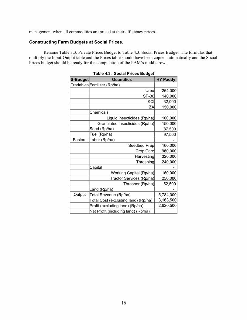
management when all commodities are priced at their efficiency prices. Constructing Farm Budgets at Social Prices. Rename Table 3.3. Private Prices Budget to Table 4.3. Social Prices Budget. The formulas that multiply the Input-Output table and the Prices table should have been copied automatically and the Social Prices budget should be ready for the computation of the PAM’s middle row.

Table 4.3. Social Prices Budget S-Budget Quantities HY Paddy Tradables Fertilizer (Rp/ha)

Urea 264,000 SP-36 140,000 KCl 32,000 ZA 150,000 Chemicals - Liquid insecticides (Rp/ha) 100,000 Granulated insecticides (Rp/ha) 150,000 Seed (Rp/ha) 87,500 Fuel (Rp/ha) 97,500

Factors Labor (Rp/ha) - Seedbed Prep 160,000 Crop Care 960,000 Harvesting 320,000 Threshing 240,000 Capital -


Land (Rp/ha) - Output Total Revenue (Rp/ha) 5,784,000

Total Cost (excluding land) (Rp/ha) 3,163,500 Profit (excluding land) (Rp/ha) 2,620,500 Net Profit (including land) (Rp/ha)

16

Appendix 4.1. Determining Export and Import Parity Prices

The social price of a tradable output or input at the wholesale market nearest to the farm gate equals the international or border price adjusted for exchange rates and domestic transportation, processing, and marketing costs. The resulting farm gate prices are called import and export parity prices or sometimes border price equivalents. The general concepts for developing export and import parity prices are shown in Table 4.1.1.

Appendix Table 4.1.1. Determining Import and Export Parity Prices

Step Import Parity Prices Export Parity Prices STEP DATA PROCESS DATA PROCESS

International Prices F.o.b. price at point of export Given C.i.f. price at point of import

Given

Freight to point of import Given Freight to point of export

Given

Insurance Given Insurance Given C.i.f. at point of import F.o.b + Freight +

Insurance. F.o.b. at point of export C.i.f - Freight -

Insurance Currency Conversions Foreign exchange rate Given Foreign exchange rate Given Foreign exchange premium Given Foreign exchange pre

mium Given

Equilibrium exchange rate ER * (1 + ERP) Equilibrium exchange rate

ER * (1 + ERP)

C.i.f. in domestic currency EER * C.i.f at point of import

F.o.b in domestic cur rency

EER * F.o.b. at point of export

Weight Conversions Weight conversion factor Given Weight conv. factor Given C.i.f. in dom. curr. and

weight C.i.f. in dom. curr. / Weight conversion factor

F.o.b. in dom. curr. and weight

F.o.b. in dom. curr. / Weight con version factor

Distribution between port & wholesale mar ket.

Local transport & mkting costs to wholesale mkt, in social prices

Given Local transport & mkting costs to wholesale mkt, in social prices

Given

Value before processing C.i.f. in dom. curr. and weight + dis trib. costs.

Value before processing

F.o.b. in dom. curr. and weight - distrib. costs.

Processing conv. factor Given Processing conv. factor Given Import parity value at whole

sale market Value before pro cessing * conver sion factor

Export parity value at wholesale market

Value before pro cessing * conver sion factor

Distribution between wholesale & farm gate

Transport, marketing, & storage costs to farm, in social prices

Given Transport, marketing, & storage costs to farm, in social prices

Given

Result Import parity value at farm gate

Import parity value at wholesale mar ket +/- distr. costs to farm gate (Deduct if output; Add if input)

Export parity value at farm gate

Export parity value at whole sale market - distr. costs to farm gate

Preparing an Import Parity Price Table. Create a table to the right of Table 4.1 on the Chapter 4 worksheet and label it Appendix Table 4.1.2. The data to be used, and the required intermediate calculations, are shown in the table below.

17

Formulas for Determining the Import Parity Price of Rice

The price of imported rice from Bangkok will serve as a starting point for deriving the import parity price for paddy in Indonesia.

1. To calculate the C.i.f. price for rice at the Indonesian port: C.i.f. at point of import = F.o.b. price at point of export + freight costs + insurance costs

2. Calculate the Equilibrium exchange rate: Exchange rate * (1 + exchange rate premium)

3. Convert international prices in dollars ($) to local currency (Rupiah). C.i.f. in domestic currency = C.i.f. at point of import * equilibrium exchange rate

4. Convert the unit of measure from tons, the usual international price unit, to kilograms.

C.i.f. (Rp/kg) = C.i.f. (Rp/ton)/1000

5. Add distribution costs between the port and the wholesale market to the weight-adjusted

c.i.f.price

6. Multiply "before processing" cost by the processing conversion factor. Adjust for the cost of milling net of the value of rice bran.

7. Adjust for the cost of distributing the commodity from the wholesale market to the farm gate.

(Because paddy is an output, the costs of distribution between the wholesale market and farm gate are deducted from the import parity value at the wholesale market.)

Table 4.2. 2. Adjustment of International Prices to Farmgate Level F.o.b. Thailand ($/ton) 150.00 Freight & Insurance ($/ton) 20.00 C.i.f. Indonesia ($/ton) 170.00 Exchange rate (Rp/$) 9,000 Exchange rate premium (%) 0% Equilibrium exchange rate (Rp/$) 9,000 C.i.f. Indonesia in domestic currency (Rp/ton) 1,530,000 Weight conversion factor (kg/ton) 1000 C.i.f. Indonesia in dom. curr. (Rp/kg) 1530.0 Transportation and handling costs to wholesale market (Rp/kg) 133 Value before processing (Rp/kg) 1663.0 Processing conversion factor (%) 0.64 Cost of rice milling net of the value of rice bran 50 Import parity value (Rp/kg) 1014.3 Distribution costs to farm (Rp/kg) 50

18

Table 4.2. 2. Adjustment of International Prices to Farmgate Level Import parity value at farm gate (Rp/kg) 964.3

Determining the Export Parity Price of Corn The social export parity price is the border price of an exportable good adjusted for transport and handling costs and revalued by the EER. The calculations for the export parity price resemble those for the import parity price, but generally work in the opposite direction. Follow the steps outlined in Table 4.1.2 to calculate Table 4.1.3, the social price of corn in Padang, assuming that corn is an exportable good. Create a new table under Appendix Table 4.1.2 and label it Table 4.1.3. Social Export Parity Price of Corn. It can be created most easily by copying Table 4.1.2 and changing the labels and computations where necessary.

Data and Assumptions for Appendix Table 4.1.3. • C.i.f. U.S. Gulf price for no. 2 yellow corn = $115/ton • Costs of insurance and freight between the U.S. and Jakarta = $17.50/ton • Official exchange rate: $1 = Rp 1644 • Foreign exchange premium = 10% • Transportation costs from port of Jakarta to wholesale market = Rp 7/kg. • Handling costs from port to wholesale market = Rp 8/kg. • Conversion of weights: 1000 kilograms = 1 ton • Farm to wholesale distribution costs= Rp 10/kg

A conversion factor is not necessary for processing corn because the commodity is sold on international markets in an unprocessed form.

Deriving the Export Parity Price for Corn in Padang. Derive the intermediate values based on the assumptions given above and the steps described in Table 4.1.2. Several of the cell formulas must be modified to account for the difference between an imported output and an exported output.

Appendix Table 4.1.3. Calculation of the Social Export Parity Price of Corn C.i.f. ($/ton) 115 Freight & Insurance ($/ton) 17.5 C.i.f. Indonesia ($/ton) 132.5 Exchange rate (Rp/$) 1,644 Exchange rate premium (%) 10% Equilibrium exchange rate (Rp/$) 1808.4 C.i.f. in domestic currency (Rp/ton) 239,613 Weight conversion factor (kg/ton) 1000 C.i.f. in dom. curr. (Rp/kg) 239.6 Transportation costs (Rp/kg) 5 Marketing costs (Rp/kg) 7 Value before processing (Rp/kg) 251.6 Processing conversion factor (%) 1

19

Appendix Table 4.1.3. Calculation of the Social Export Parity Price of Corn Import parity value (Rp/kg) 251.6 Distribution costs to farm (Rp/kg) 10 Import parity value at farm gate (Rp/kg) 241.6

Linking Tables in the Spreadsheet Link the results of the import parity price calculations for rice directly into the Social Prices table, overwriting the preliminary values entered in Chapter 4. To link the relevant cells, move to the Social Prices Table, delete the existing entry, and click on =. Then select the appropriate (final price) entry from the parity price calculation table. Click OK. Sensitivity Analysis The spreadsheet is now integrated so that sensitivity analysis on international prices and exchange rates can be reflected in the social budgets. How does the social profitability for the paddy system change when: 1) The exchange rate premium rises to 30%? 2) The international price of rice rises by 25%? The Import and Export Parity Prices tables assume an exchange rate premium of 0 percent, which means that the exchange rate is not overvalued. Although many developing countries experience overval-ued exchange rates, it is often difficult to ascertain the exact amount of the premium. Hence, it is desirable to test the results of different EER assumptions. Determining an international price of rice is also difficult. Care must be taken to ensure that the variety and quality of the rice from the world market is the same as the domestic rice with which it is being compared. Hence the international price is a prime target for sensitivity analysis. Summary This appendix reviewed the process for calculating the social prices of tradable commodities. Data are required for international commodity prices, distribution costs between various stages of the marketing chain, exchange rates, weight conversions and processing factors. The steps involved in transforming these data into parity prices were outlined in Table 4.1.1. Distinctions were drawn between the calculations for imported outputs, imported inputs, and exports of both outputs and inputs. For purposes of illustration, sample data were provided for only two of these categories, permitting the construction of tables for paddy (occasionally an imported output) and corn (occasionally an exported output). The import and export parity prices so derived are the social prices faced by farmers. To test the effects of changes in international prices and exchange rates on social profitability, these results were linked to the original Social Prices table constructed in Chapter 4. Although the computations are straightforward, data requirements are often formidable. For example, in identifying the f.o.b. and c.i.f. prices in international markets, it is usually difficult to ensure equivalence in specifications (e.g., quality) between the traded product and the domestically available product. Even small mistakes in establishing the comparability of products can swamp large errors in input-output coefficients.

20

Appendix 4.2. Nontradable Good Prices

Analysis of Non-Tradable Services Previous chapters have ignored the issue of nontradable services such as machine rentals, transportation, processing, and handling. Collecting data for these nontradable services is one of the most challenging, and often frustrating, exercises in agricultural policy analysis. Because the information is difficult to collect and, once gathered, may only have a marginal impact on the results, analysts frequently resort to broad assumptions about the data, using sensitivity analysis to verify that these assumptions would not do violence to their conclusions. But as Monke and Pearson point out in their Chapter 10 ("Postfarm Budgets and Analysis"), market imperfections or policy divergences in nontradable goods and services should not be treated in a cavalier fashion. In theory, the costs of all nontradable inputs (goods and services) should be decomposed into their tradable inputs and domestic factor cost components. These costs, standardized on units such as hours or measures of volume or weight, then can be substituted into the appropriate cells of the Private and Social prices tables. The current chapter focuses on policy divergences in the tradable component of tractor services and illustrates how these divergences affect private and social budgets.

Decomposing Tractor Costs In Chapter 2, tractor services were considered as domestic factors rather than tradable components of the farm budget. As such, the labor associated with tractor services was included in various farming operations; the capital cost associated with these services was included in the capital account. But the rental price of these machines masks a significant tradable component in the form of machine depreciation, fuel, and grease and oil. This exercise decomposes tractor services and assigns the tradable, labor, and capital components to their respective accounts in the private and social budgets. As with the linking of import and export parity prices to the Social Prices table (last chapter), the steps involved in identifying the tradable portion of nontradable services are not conceptually difficult. The process of modifying the spreadsheet, however, requires several calculations and careful adjustments to early tables. The first step is to identify the aspects of tractor services that are tradable. In this example, the tradable component consists of three parts -- the tractor itself, fuel, and grease and oil. The nontradable component consists of two parts -- the use of labor for repairs, maintenance, and management operations, and the working capital required to finance operational expenses. Second, one needs to determine a meaningful unit of tractor use (usually taken as the tractor service hour) and the quantity of each tradable and nontradable component used during that time. For example, how much tractor capital is used up during one hour of tractor use (depreciation)? How much fuel is used? Grease and oil? Labor? Capital? Third, appropriate private and social prices for these quantities must be found. For tradables, social prices are derived in a manner similar to that used to calculate import and export parity prices in the last chapter. In this particular example, tractors, fuel, and grease/oil are imported and thus the calculations follow the steps used to derive import parity prices. In general, private prices for both tradables and nontradables are those observed in the market place. In this example, the private prices for tradable goods have been further decomposed to highlight the effect of government interventions and the

21

assumptions concerning depreciation. For nontradables, private prices are observed in the market and thus are taken as given. In both cases, private prices are presented on a per tractor hour basis. Once the quantities and prices for the newly defined components of tractor services have been determined, they must be linked back into the initial budgetary calculations. The Input-Output table must be expanded to incorporate rows for tradable tractor services, tractor labor, and tractor capital. The original figures for hours of tractor services (previously lumped under the capital account of the I-O table) must be moved to the tradables portion of the table. There they serve as the base for calculating the hours of repair and maintenance labor (R & M) used per hectare and working capital required for tractor services per hectare. Next, similar rows are inserted in the Private Prices and Social Prices tables. Private and social price data must be linked from the table containing the various "tractor services" calculations. Once the appropriate lines and formulas are inserted, the Private Budget and Social Budget tables recalculate automatically. Sensitivity analysis can be undertaken to evaluate the importance of decomposing the tradable components of domestic services.

Modifications to the Spreadsheet

Step 1: Creating the Tractor Inputs Table. Retrieve PAMTutorial. Insert a new worksheet, rename it Nontradables. Create a data Table 4.2.1 called Tractor Inputs. Enter the quantity of each of the tradable components (tractors, fuel, grease/oil, and nontradable components (R&M labor, working capital)) used per tractor hour. The R&M coefficient describes the amount of repair, maintenance, and administrative labor used by the vendor to deliver one hour of tractor services. The working capital coefficient describes the amount of working capital used by the vendor to deliver one hour of tractor services.

Table 4.2.1 Tractor Inputs Items # of Units per Tradable Components Tractor Hour Tractor (hours) 1 Fuel (liters) 0.135 Grease and oil (liters) 0.0052 Nontradable Components R&M Labor (hours) 0.015 Working Capital (Rupiahs) 500

Step 2: Creating the Tractor Prices Table

Create the Tractor Prices table below the Tractor Inputs table. It resembles the Import Parity table in structure and in arithmetic logic (i.e., the calculations are very similar). The necessary additional labels and formulas to incorporate duties, subsidies, time conversions, and depreciation can then be added. (The labels in the social price portion of the Tractor table are identical to those in the private portion.) The costs of tradable tractor services are constructed along the same lines as the commodity import parity prices. F.o.b. prices obtained from exporting countries are the point of departure if local estimates of the c.i.f. prices in foreign currency are unavailable. The likelihood that the latter can be found is very high since local importers will know what their landed costs are.

22

Table 4.2.2 Tractor Prices

Private Prices Social Prices

Tractor Fuel Grease, Oil Total Tractor Fuel Grease, Oil Total

(machine) (liters) (liters) (machine) (liters) (liters) F.o.b. ($/Unit) 5000 0.2 3.4 5000 0.2 3.4

Freight and Insurance ($/Unit) 400 0.04 0.15 400 0.04 0.15

C.i.f. ($/Unit) 5400 0.24 3.55 5400 0.24 3.55

Official Exchange Rate (Rp/$) 1644 1644 1644 1644 1644 1644

Exchange Rate Premium (%) 0% 0% 0% 10% 10% 10%

Equilibrium Exchange Rate (Rp/$) 1,644 1,644 1,644 1,808 1,808 1,808

C.i.f. (Rp/Unit) 8,877,600 395 5,836 9,765,360 434 6,420

Domestic Duties (%) 0.4 0.4 0.3 0 0 0

Domestic Subsidies (%) 0 0 0 0 0 0

Import Parity at Border (Rp/tractor) 12,428,640 552 7,587 9,765,360 434 6,420

Expected Life (hours of life/tractor) 25,000.00 n.a. n.a. 25,000.00 n.a. n.a.

Cost per hour transportation (Rp/hr) 497 n.a. n.a. 391 n.a. n.a.

Transportation (Rp/unit) 10 1 3 10 1 3

Farm Gate Value (Rp/unit) 507 553 7,590 0 401 435 6423 0

Total Tractor Service Hour (Rp/hr) 507 74.7 39.5 621.1 401 59 33 493

• Calculate the Import value at border as the c.i.f. price plus the Rupiah value of domestic duties less the Rupiah value of domestic subsidies. Because duties and subsidies are proportions, the formula is:

• Prorate the total capital cost of the tractor over its useful life:

• Calculate the Total cost per tractor service hour for each of the tradable components as the product of its Farm gate value and the # of units per tractor service hour (found in the Tractor Inputs table).

• The social price formulas are identical to those for private prices. So too are the data, with the exception of the Domestic duties and Equilibrium exchange rate.

The differences between private and social costs in tractor services originate from the same sources as the divergences in the agricultural sector. For example, many governments subsidize tractor services by permitting tractor dealers to import tractors and spare parts using foreign exchange obtained at an overvalued exchange rate. Gasoline and diesel fuel are also frequently subsidized. (No subsidies are shown in the current example.) Conversely, imports of machines are heavily taxed to encourage and protect domestic production, especially of smaller machines like two-wheeled tractors. Imports of oil are also significantly taxed instead of subsidized. For both machines and production inputs such as fuel, the degree of taxation is somewhat offset by granting foreign exchange allocations at a cost below the equilibrium exchange rate. The offsetting effects of an overvalued currency and import duties can be seen from the private and social price calculations in Table 4.2.2.

Step 3: Modifying the Input-Output, Prices, and Budget Tables

23

The structure of the Input-Output, Private Prices, Private Budget, Social Prices, and Social Budget tables are each modified in an identical fashion, by inserting a new row in the tradables and labor sections. (The capital section already includes tractor services). It is easiest to complete all structural changes on each table before progressing to the next. A sample drawn from the I-O table is shown in Table 4.2.3. Consistent with the original design of these tables, the units of measure depend on the table, and in some cases, on the nature of the input. Apply the following steps to each of the five tables cited.

• Modify the tradables section by inserting a row entitled Tractor Services (hr/ha).

• Modify the labor section by inserting a row entitled Tractor R&M.

• In the I-O table only, move the hours from the Tractor services row currently in the capital section to the new tradables row for these same services. These coefficients describe the number of tractors hours used by each commodity. The Tractor Services row in the capital section and the Tractor R&M row in the labor section should be devoid of data. New data will be written in later.

• Repeat the first 2 steps for the Private Prices, Private Budget, Social Prices, and Social Budget tables. Adjust units according to the nature of the table (e.g., hr/ha for the I-O table, Rp/hr for the Prices tables, and Rp/ha for the Budget tables.) Note that Tractor Services Capital is now on a percent basis in the Prices tables (rather than Rp/hr).

Table 4.2.3. Physical Input-Output

I-O Quantities HY Paddy Tradables Fertilizer (kg/ha)

Urea 240 SP-36 100 KCl 20 ZA 150 Chemicals Liquid pesticide (liters/ha) 3 Granulated pesticide (kg/ha) 15 Seed (kgs/ha) 35 Tractor Services (hr/ha) Fuel (liters/ha) 65

Factors Labor (hr/ha) Seedbed Prep 100 Crop Care 600 Harvesting 200 Tractor R & M Threshing 150 Capital

Working Capital (Rp/ha) 2,000,000 Tractor Services (Rp/ha) 20 Thresher (hr/ha) 35


24

Step 4: Linking the Tractor Tables to the Input-Output and Prices Tables

The Tractor Inputs table contains information on the quantities of tradables and nontradables used per tractor service hour. The Tractor Prices table contains the private and social prices of the tradable components (the tractor, fuel, and grease/oil) per tractor service hour. These must be converted to the unit used throughout this analysis -- hectares -- and linked to the appropriate tables. The prices of labor and capital have not changed and are already included in the prices tables.

• In the labor section of the I-O table, calculate Tractor R&M labor per hectare by multiplying the number of hours of Tractor Services per hectare (in the tradables section of the I-O table) by R&M labor per tractor service hour (on the Tractor Inputs table). • In the capital section of the I-O table, calculate Tractor Services capital per hectare by multiplying the hours of Tractor Services per hectare (in the tradables section of the I-O table) by Working Capital per tractor service hour (on the Tractor Inputs table). • Format the new rows to be consistent with other data presented in the I-0 table.

• In the tradables section of the Private Prices table, calculate the private price of Tractor Services per hectare as total Cost per Tractor Service Hour, aggregated across Tractor Services, Fuel, and Grease/Oil (on the Tractor Prices table). • In the labor section of the Private Prices table, copy the private price of Tractor R&M per hectare directly down from the wages figure in the preceding row.

• In the capital section of the Private Prices table, copy the private price of Tractor Capital per hectare directly down from the season interest rate in the preceding row.

• Format the new rows to be consistent with other data presented in the table.

• Calculate the social price of tradable Tractor Services, Tractor R&M labor, and Tractor Services capital in the same manner as that used for the private price, referencing data in the Social Prices section of the Tractor Services table.

• Update the Private and Social Budget tables by copying the formula in adjacent rows to those for the tradable component of tractor services and the labor component of tractor services. The capital component of tractor services should have adjusted automatically.

Save the spreadsheet as PAMTutorial

Sensitivity Analysis Integrating the results of the decomposition into the existing tables is the most time-consuming part of the exercise. However, such integration is highly desirable because it simplifies the sensitivity analysis of various types of policy proposals. Once the template has been properly implemented, it will be easy to see if significant changes in the international price of tractors has an impact on commodity PAMs. If the PAMs have been done correctly in the earlier exercises, changes in the Tractor

25

Decomposition table should be automatically reflected in the PAMs. To gain a better understanding of the relative importance of nontradable service decomposition, perform the following sensitivity analysis. 1) Tractor prices double. 2) Fuel prices triple. Do the PAM results change much? What do the results of this sensitivity analysis imply for data collection priorities?

Summary This appendix has shown how to decompose nontradable services into their tradable and domestic factor components. The illustration was simplified for ease of presentation, but the difficulty in computing costs of nontradable services should not be underestimated. Due to the inherent problems of estimating the social costs of services, it is often useful to assess their importance in the budget of individual commodities before embarking on a complete analysis. This can be done by computing the value of nontradable services as a share of total costs and by performing sensitivity analyses.

26

Chapter 5: Policy and Market Failures

Chapter 5 contains a series of PAM exercises. The first focuses on a single commodity system (rice) using the budgets developed in Chapters 3 and 4. Complete information on competing alternatives is not available in this example and hence profits include returns to land as well as management. The second rice PAM incorporates information about the opportunity cost of soybeans, a crop that competes with rice for land. This requires adding an additional Land column in the rice PAM and is called a “farming systems” PAM. The third exercise investigates the methodology for computing PAMs when the commodity is a perennial, i.e., where planting, production, and harvesting take place over a number of periods. Vanilla is used as a example. Single Commodity PAM for Rice The first step in computing a single-commodity PAM for High Yielding Paddy is to insert a new worksheet in the PAMTutorial workbook. Rename it simply PAMs. Label the columns and rows to create a typical PAM table. (Table 5.1 below.)

Table 5.1. PAM for Indonesian Rice

Revenues Tradable Domestic Resources Profits Inputs Labor Capital

Private 7,230,000 966,000 1,680,000 402,500 4,181,500 Social 5,784,000 1,021,000 1,680,000 462,500 2,620,500 Divergences 1,446,000 (55,000) - (60,000) 1,561,000

To compute the elements of the PAM, utilize the methods used earlier to create the budget tables. Select the cell Private Revenue cell and click on the equals (=) sign in the Formula Bar. Then click on the Total Revenue cell for High Yielding paddy in the Private Budget table (Table 3.3 under the Private Budget tab). Click on O.K. Do the same for the social output entry. Completing the remaining entries requires slightly more effort. To compute the Private Tradable Costs cell, select the cell and begin to write the summation function in the Formula Bar by first clicking on the = sign, then typing SUM and an open parenthesis. The completed entry is =SUM(. A dialog box will pop-up requesting the range over which the function should sum. Click on the P-Budget tab and select the input items (Urea through fuel) that constitute paddy input costs. (If the dialog box obscures the view of the relevant data, drag it to the bottom of the page.) Complete the formula by adding a closing parenthesis. Then click on OK. Use the same procedure to compute the labor inputs cell and the capital inputs cell. Select the cell to be completed, make sure it is empty, click on the = sign, type SUM(, complete the range by going to the appropriate worksheet and selecting the relevant range, in this case labor and capital, type in a closing parenthesis, and click on OK. Once data from the budget tables have been entered for Table 5.1, the profits column and the divergences row can be computed. To complete the profits column, subtract the sum of the Inputs, Labor,

27

and Capital cells from the Revenue cell. To compute the divergences row, subtract social entries from private entries. Remember to utilize the copy command as much as possible.

Questions Interpret the results of the high productivity paddy PAM. To what extent do policies affect paddy prices? What about input subsidies?3 The positive divergence in tradable outputs indicates that farmers are receiving more than the social value for their crop. They are, in effect, being subsidized by the amount of the divergence. The negative divergence in tradable inputs reflects a subsidy to farmers for use of these inputs. Farmers do not pay the full social cost of these inputs and the divergence represents the cost to the government. The difference between the private and social interest rate causes the divergence in the capital column. (For a more detailed analysis of the PAM, see Chapter 5 of the PAM book.) Farming Systems PAM The previous PAM was created under the assumption that the social opportunity cost of land could not be identified. However, in many areas of Indonesia, soybeans can also be grown on land used for rice. Soybean profits provide an opportunity cost for land that can be incorporated into a complete “farming systems” rice PAM. Table 5.2 is derived from the same type of budget analysis that was illustrated in Chapters 3 and 4. To add the PAM to the Excel workbook, go to the PAMs tab and copy Table 5.1 below itself. Copy the figures for revenues and costs into the new table. Profits and divergences will be computed automatically.

Table 5.2. PAM for Soybeans

Revenue Tradable Domestic Resources Profits

Inputs Labor Capital Private 2,824,000 168,000 579,325 85,942 1,990,733 Social 2,468,500 168,000 579,325 112,099 1,609,076 Divergences 355,500 - - (26,157) 381,657

The farming systems PAM (Table 5.3) requires the addition of a column that reflects the price of land as derived from the profits of growing soybeans. To compute the new PAM, copy Table 5.1 below Table 5.2 and label it Table 5.3 Farming Systems PAM for Rice. Rename the next to last column Land and enter the profit values obtained from the soybean PAM. The substantial private and social profits for rice after the opportunity cost of land has been subtracted underscores the comparative advantage of rice in the cropping pattern. (Using rice profits to compute a farming systems PAM for soybeans would have produced negative private and social profits for soybeans.)

Table 5.3. Farming Systems PAM for Rice

Revenue Tradable Domestic Resources Profits

3 Chapter 12, pp. 226-236, of Monke-Pearson provides detailed interpretations of a number of PAMs that can serve as models for interpreting the high productivity paddy PAM.

28

Inputs Labor Capital Land Private 7,230,000 966,000 1,680,000 402,500 1,990,733 2,190,767 Social 5,784,000 1,021,000 1,680,000 462,500 1,609,076 1,011,424 Divergences 1,446,000 (55,000) (60,000) 381,657 1,179,343

Multi-Period PAM Previous PAMs have been based on seasonal crops. These dominate Indonesian agriculture. However, there are a number of commodities whose planting and harvesting takes place over time. Examples include such crops as rubber, cloves, and vanilla, as well as investments in livestock production. Computing PAMs for commodities that stretch over a number of periods requires constructing a PAM for each period, then computing the net present value of the entire series. Discounting is necessary because the value of future costs and returns is less than the value of costs and returns measured in the present. T he fact that alternative returns to revenues and expenditures —their opportunity cost—increases at a compound rate, e.g., bank account deposits, needs to be accounted for in the multi-period PAM. The formula for computing the NPV for revenue is:

∑= +

=n

tt

tR i

RNPV

1 )1( where i is the discount (interest) rate and t is the number of time periods over which the commodity is grown. Table 5.4 shows the budgets for vanilla over the 10-year period that comprises the normal cycle of production. In the first two periods, the crop requires inputs and resources, but yields no revenues. Output increases until the 5th year when the crop reaches maturity. After than, output declines until the 10th year when the vanilla is hardly worth harvesting.

• To create Table 5.4, copy Table 5.1 below Table 5.3, add the additional rows that reflect budgets for each successive year, and copy the data for revenues and costs. (Data are given in Rps (000,000) to minimize typing.) The profits column will be computed automatically.

• To compute the net present value of the 10-year series, click on the cell below the last

element of the series and, after clicking on =, type NPV(. In the pop-up box labeled “Rate,” select the cell address for the cell containing the interest rate. In the cell labeled “Value 1,” select the range for the series. Click on ok.

• Make the cell address for the interest rate absolute (F4) and copy the formula into the

remaining columns.

Table 5.4. Multi-period Vanilla Budgets (Private Prices in Rps 000,000)

Year Revenue Tradable Domestic Factors Profit

29

Inputs Labor Capital Interest rate 15%

1 0.0 3.0 5.0 1.0 -9 2 0.0 0.6 6.0 1.0 -8 3 16.0 0.9 9.0 2.0 4 4 35.0 1.1 9.0 2.0 23 5 39.0 1.0 9.0 2.0 27 6 31.0 0.8 9.0 2.0 19 7 33.0 1.0 8.0 2.0 22 8 26.0 1.3 6.0 1.0 18 9 20.0 0.3 6.0 1.0 13 10 11.0 0.3 5.0 1.0 5

NPV 92.6 6.1 36.2 7.6 43

Compute the second row of the PAM (social prices) by copying Table 5.4 below itself and labeling it Table 5.5. Multi-Period Budgets (Social Prices in Rps. 000,000). Change the interest rate to 24 percent and type the data in the new table. Compute the NPV for each column using the method described above.

Table 5.5. Multi-period Vanilla Budgets (Social Prices in Rps 000,000)

Year Revenue Tradable Domestic Factors Profit Inputs Labor Capital

Interest rate 18% 1 0.0 3.0 5.0 2.0 -10 2 0.0 0.6 6.0 2.0 -9 3 15.0 0.8 9.0 2.0 3 4 32.0 1.0 9.0 3.0 19 5 36.0 0.9 9.0 2.0 24 6 29.0 0.7 9.0 2.0 17 7 31.0 0.9 8.0 2.0 20 8 25.0 1.0 6.0 2.0 16 9 18.0 0.3 6.0 2.0 10 10 11.0 0.3 5.0 1.0 5

NPV 74.7 5.3 32.3 9.3 27.7

Create Table 5.6 by copying Table 5.1 below Table 5.5 and label it Table 5.6 Multi-Period Vanilla PAM. In the data cells of the PAM, enter the NPV calculated for each of the elements in the private and social budgets. (The profits and divergences should be computed automatically.) The PAM’s results indicate the total profits and the total policy and market related divergences for the period.

Table 5.6. Multi-period Vanilla PAM (Rps. 000,000)

Revenue Tradable Domestic Factors Profit Inputs Labor Capital

30

Private 93 6 36 8 43 Social 75 5 32 9 28

Divergence 18 1 4 (2) 15

The multi-period PAM is interpreted in the same way as a single-period PAM. Table 5.6 shows that producers are receiving substantial subsidies through government policies, either in the direct purchase of the crop from trade policy that affects the output price. Sensitivity Analysis How sensitivity is the analysis to the discount used to compute the NPV? Would make any difference to the PAM conclusions if, instead of 15% , the rate was 5%? What if it was 25%?

31

Appendix 5.1. Computing Summary Ratios

To compare the profitability and efficiency of different crops, a common numeraire must be used throughout the analysis. The use of ratios is a convenient method of avoiding the problem of a common numeraire, particularly when the production processes and outputs are very dissimilar. Several useful ratios that provide information on private and social profitability can be derived directly from the data in the policy analysis matrix. Both the numerator and the denominator of each ratio are PAM entries defined in domestic currency units per physical unit of the commodity. Therefore, the ratio is a pure number free of any commodity or monetary designation.4 In this part of the exercise, the results from the previous PAMs will be used to calculate the nominal protection coefficient (NPC), the effective protection coefficient (EPC), and the domestic resource cost coefficient (DRC). The ratios will be calculated in a summary table so that the results can be compared easily between crops. The summary table is also convenient for conducting sensitivity analysis on the results. To create the summary table, Insert a new worksheet in the workbook and rename it Ratios. The Ratio Table

The Nominal Protection Coefficient (NPC) The bottom row of the PAM indicates the extent of commodity and factor market divergences in the production of each crop. In the absence of market failures, this row measures the effects of distorting policy on inputs and outputs. The nominal protection coefficient, defined by the ratio of private commodity prices and social commodity prices, compares the impact of government policy (or of market failures that are not corrected by efficient policy) between different crops.5

• Calculate the NPC for tradable outputs (i.e., crop output) using the formula shown below.

NPCO = Revenue in private prices / Revenue in social prices

• Select the cell to be completed, click on the = sign, then on the PAM tab. Click on the private output cell, type in /, then click on the social output cell. Click on OK. Utilize the same method to compute the NPCI. •

Table 5.1.1 Summary Ratios NPC EPC DRC Outputs Inputs

High-Yield Paddy 1.25 0.946 1.315 0.450

An NPC for tradable outputs greater than 1 shows that the market price of the output exceeds the social price. The farmer receives an implicit output subsidy from policies affecting crop prices.

4 For a more detailed discussion of various summary ratios including the DRC, see M-P, pp. 25-29. 5 "Efficient" policies are interventions deliberately introduced to offset market failures. For a discussion of policies that promote food security in developing countries where imperfect capital and insurance markets make it difficult to obtain a desired protection against risk, see M-P, pp. 53-54.

32

• Calculate the NPC for tradable inputs for shown in Table 5.1.1 from its corresponding PAM.

NPCI = Cost of tradable inputs at private prices/ cost of tradable inputs at social prices

An NPC for tradable inputs less than 1 indicates that market prices of inputs fall below the price that would result in the absence of policy. This ratio reveals the presence of input subsidies, taxes, trade restrictions or an inappropriate exchange rate.

The Effective Protection Coefficient (EPC) The effective protection coefficient, defined as the ratio of value added in private prices to value added in social prices, more completely measures incentives to farmers. The EPC indicates the combined effects of policies in the tradable commodities markets. This is a useful measure because input and output policies, such as commodity price supports and fertilizer subsidies, often constitute part of a comprehensive policy package. For example, governments frequently reduce the price of outputs but then subsidize inputs in an effort to encourage the adoption of new technology.

• Calculate the EPC cell in Appendix Table 5.1.1 for each of the commodities using the

formula:

EPC = (Revenue – Cost of tradable inputs) in private prices / (Revenue – Cost of tradable inputs) in Social Prices

• To compute the values for the EPC cells, use the methods described earlier for computing the

values for the NPCs. Select the cell, click on =, click on the PAMs tab, and complete the formula.

An EPC greater than 1 indicates positive incentive effects of commodity policy (a subsidy to farmers) whereas an EPC less than 1 shows negative incentive effects (a tax on farmers). Both the EPC and the NPC ignore the effects of transfers in the factor market and therefore do not reflect the full extent of incentives to farmers.

The Domestic Resource Cost Coefficient (DRC) The domestic resource cost coefficient measures the efficiency, or comparative advantage, of crop production. If the social returns to land cannot be identified clearly because full information about alternatives is lacking, the DRC may be calculated with respect to labor and capital only. The DRC serves as a proxy measure for social profits. It is calculated by dividing the cost of labor and capital by value-added at social prices.

• Calculate the DRC for rice as:

DRC = (Labor costs + capital cost) in Social Prices/ (Revenues – Cost of tradable inputs) in Social Prices

Where the opportunity cost of land can be clearly identified, the DRC is calculated by including the cost of land (i.e., the social profitability) of the next best alternative crop. The resulting DRC reflects Use the methods described above to compute the values for Appendix Table 5.1.1 under the

33

Ratios tab. The DRC will be positive unless the social value added in crop production is negative. However, DRCs greater than one indicate that the value of domestic resources used to produce the commodity exceeds its value added in social prices. Production of the commodity, therefore, does not represent an efficient use of the country's resources. DRCs less than one imply that a country has a comparative advantage in producing the commodity. Values less than one mean that the denominator (value added measured at world prices) exceeds the numerator (the cost of the domestic resources measured at their shadow prices). Save the spreadsheet as PAMTutorial.

34

Chapter 6. Benefit-Cost Analysis

Introduction Benefit-cost analysis is a powerful tool for evaluating the economic desirability of capital investments. A major portion of this type analysis for a particular farming system has already been completed when the PAMs for that system are finished. What remains is (1) calculating a second, new PAM that incorporates the changes in the farming system resulting from the capital investment, (2) determining the size and composition of the capital investment, and (3) computing the discounted B-C ratios and internal rates of return (IRRs) that arise from the stream of differences between the old and new PAMs. To begin, it is important to note that the budgets thus far calculated in Chapters 3 and 4 have been drawn from acreages that have “good” water control. That is, the PAM reflects a situation in which an irrigation project has already been completed at some time in the past. It will be referred to in Chapter 6 as the “with project” PAM. It follows that, for the purpose of investigating the returns to constructing a new irrigation project, the missing information concerns the production system that is currently characterized by “poor” water control—a “without project” PAM. To some, this may seem to be a peculiar order of calculation, but project evaluation is all about the difference between the with and without condition. It does not matter which calculation is done first. In this case, the example benefits from information about the with project PAM obtained from previous work and continues from there. Given that the with project PAM already exists, the first step is to create a worksheet that reflects this previously completed work. Then a second PAM that describes a production system that has not yet had the benefits and costs of machinery, land leveling, and ditching must be developed. Such a system falls into the Indonesian category of a “medium” or “poor” water control. Data collected in the field indicate that it is likely to yield considerably less paddy/hectare, say, approximately 5,000 kgs/ha instead of the 6,000 kgs/ha expected in areas having good water control. To repeat: The good water control area from which the previous manual exercises have been drawn will be called the with project area. At some point in the past, the necessary leveling, structure construction, and channeling deepening were completed. The poor control area is less fortunate and the land is more uneven, the structures less precise, and the water less certain. This more backward area will be called the “without” project site. The incremental benefits from the project are obtained by subtracting the poor area (without project) from the improved with project: case.6 The period-specific stream of incremental costs and benefits, including investment costs, yields a “cash flow” that will be analyzed to determine the economic desirability of the proposed investment. Chapter 6 is divided into a series of steps: 6 Price Gitinger’s book, The Economic Analysis of Agricultural Projects, provides a more detailed guide to the con-cepts and the organization of the IRR computations. (The book is on-line at http://www.stanford.edu/group/FRI/ indonesia/documents/gittinger/Output/title.html .) This chapter contains an overview of these concepts, along with numbers that provide a concrete example of their application.

35

1. transferring the private and social budgets for the with project case to the B-C data worksheet.

2. computing the private and social budgets for the without project case,

3. subtracting the with from the without project budgets to compute a flow of incremental net revenues,

4. estimating the cost of the investment being investigated,

5. computing the discounted B-C (benefit-cost) ratio or the IRR (internal rate of return) for the capital expenditure.

With Project at Private and Social Prices

Private Prices

As noted above, the project’s return lies in the incremental benefits – the difference in profits between farming systems with and without investments. An accurate characterization of the without project case is just as important as the projection of the benefits expected from the project implementation. Theoretically, at least, overly pessimistic views of what would transpire in the absence of a project can be as important in producing inflated B-C ratios and IRRs as overly optimistic views of what the project is likely to accomplish. It is the difference between the two budgets that determines project benefits. Create a new worksheet and label it B-C Data. Copy Tables 3.1-3.3, completed previously, into the new worksheet. These will form the basis of the with project calculation. Rename the tables as follows:

Table 6.1. Physical Input-Output (Good Control) I-O Quantities HY Paddy

Tradables Fertilizer (kg/ha) Urea 240 SP-36 100 KCl 20 ZA 150 Chemicals Liquid pesticide (liters/ha) 3 Granulated pesticide (kg/ha) 15 Seed (kg/ha) 35 Fuel (liters/ha) 65


Working Capital (Rp/ha) 2,000,000 Tractor Services (hr/ha) 20

36


Thresher (hr/ha) 35 Land (ha) 1

Output (kg/ha) 6,000

Create Table 6.2 in the new worksheet. It is identical to Table 3.2. (Private and social prices are assumed to remain unchanged in the with and without project conditions.)

Table 6.2. Private Prices (Good Control) P-Prices Quantities HY Paddy





Create Table 6.3. It is the same as Table 3.3.

Table 6.3. Private Prices Budget (Good Control) P-Budget Quantities HY Paddy Tradables Fertilizer (Rp/ha)

Urea 264,000 SP-36 140,000 KCl 32,000 ZA 150,000 Chemicals - Liquid insecticide (Rp/ha) 75,000 Granulated insecticide (Rp/ha) 120,000 Seed (Rp/ha) 87,500

37

Table 6.3. Private Prices Budget (Good Control) P-Budget Quantities HY Paddy

Fuel (Rp/ha) 97,500 Factors Labor (Rp/ha) -

Seedbed Prep 160,000 Crop Care 960,000 Harvesting 320,000 Threshing 240,000 Capital -




Social prices In the space directly below the newly created Private Prices tables, copy the Tables 4.1-4.3 completed in the previous social budget worksheet. Utilize the technique applied in the previous section to create data tables for with project (good control) at social prices. Table 4.1 becomes Table 6.4 Physical Input-Output (Good Control).


Tradables Fertilizer (kg/ha) Urea 240 SP-36 100 KCl ZA 150 Chemicals Liquid pesticide (liters/ha) 3 Granulated pesticide (kg/ha) 15 Seed (kg/ha) 35 Fuel (liters/ha) 65



Land (ha) 1

20

38


Output (kg/ha) 6,000

Rename Table 4.2 to Table 6.5. Social Prices (Good Control).

Table 6.5. Social Prices (Good Control) S-Prices Quantities HY Paddy Tradables Fertilizer (Rp/kg)






Rename Table 4.3 to Table 6.6. Social Budget (Good Control)

Table 6.6. Social Prices Budget (Good Control) S-Budget Quantities HY Paddy Tradables Fertilizer (Rp/ha)

Urea 264,000 SP-36 140,000 KCl 32,000 ZA 150,000 Chemicals - Liquid insecticides (Rp/ha) 100,000 Granulated insecticides (Rp/ha) 150,000 Seed (Rp/ha) 87,500 Fuel (Rp/ha) 97,500

Factors Labor (Rp/ha) -

39

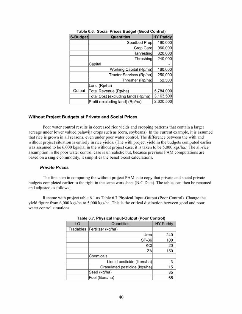
Table 6.6. Social Prices Budget (Good Control) S-Budget Quantities HY Paddy

Seedbed Prep 160,000 Crop Care 960,000 Harvesting 320,000 Threshing 240,000 Capital -



Total Cost (excluding land) (Rp/ha) 3,163,500 Profit (excluding land) (Rp/ha) 2,620,500

Without Project Budgets at Private and Social Prices Poor water control results in decreased rice yields and cropping patterns that contain a larger acreage under lower valued palawija crops such as (corn, soybeans). In the current example, it is assumed that rice is grown in all seasons, even under poor water control. The difference between the with and without project situation is entirely in rice yields. (The with project yield in the budgets computed earlier was assumed to be 6,000 kgs/ha; in the without project case, it is taken to be 5,000 kgs/ha.) The all-rice assumption in the poor water control case is unrealistic but, because previous PAM computations are based on a single commodity, it simplifies the benefit-cost calculations.

Private Prices

The first step in computing the without project PAM is to copy that private and social private budgets completed earlier to the right in the same worksheet (B-C Data). The tables can then be renamed and adjusted as follows: Rename with project table 6.1 as Table 6.7 Physical Input-Output (Poor Control). Change the yield figure from 6,000 kgs/ha to 5,000 kgs/ha. This is the critical distinction between good and poor water control situations.

Table 6.7. Physical Input-Output (Poor Control) I-O Quantities HY Paddy

Tradables Fertilizer (kg/ha) Urea 240 SP-36 100 KCl 20 ZA 150 Chemicals Liquid pesticide (liters/ha) 3 Granulated pesticide (kgs/ha) 15 Seed (kg/ha) 35 Fuel (liters/ha) 65

40





Change Table 6.2 in the copied budgets to Table 6.8 Private Prices (Poor Control)

Table 6.8. Private Prices (Poor Control) P-Prices Quantities HY Paddy





Change Table 6.3 of the copied budgets to Table 6.9 Private Prices Budget (Poor Control). The formulas, along with the data in the previous tables, have been copied and the budget table will be computed automatically.

Table 6.9. Private Prices Budget (Poor Control) P-Budget Quantities HY Paddy Tradables Fertilizer (Rp/ha)

Urea 264,000

41

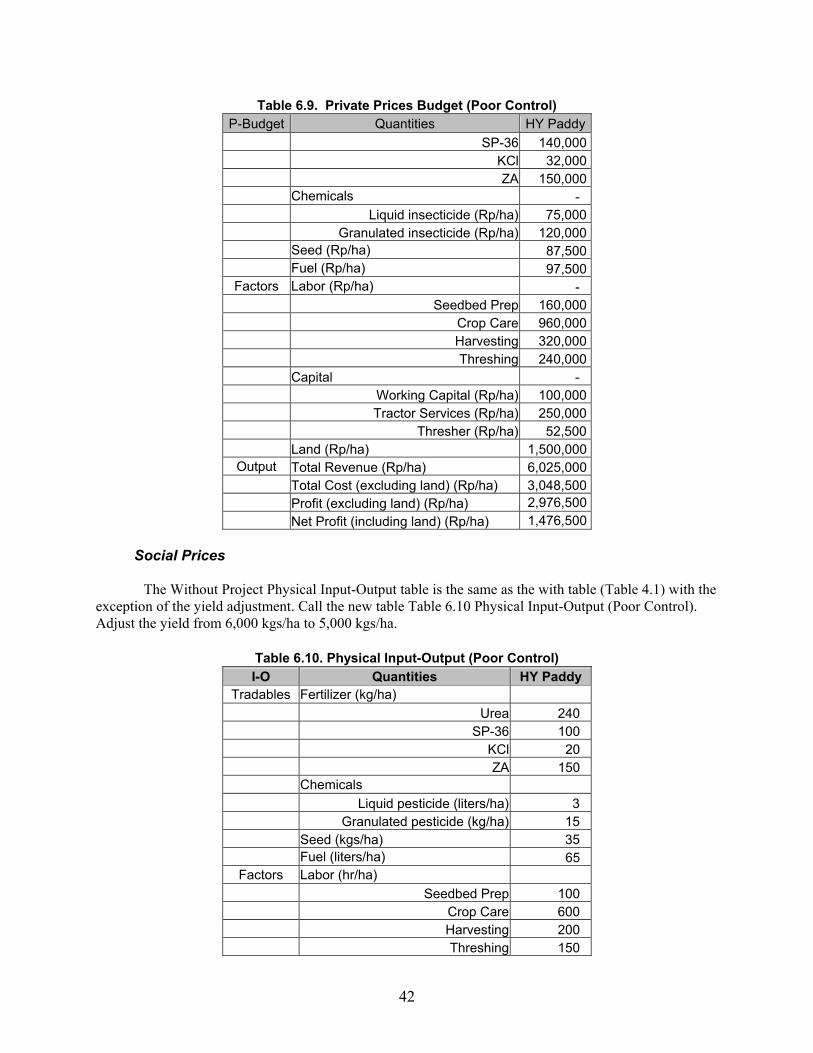
Table 6.9. Private Prices Budget (Poor Control) P-Budget Quantities HY Paddy

SP-36 140,000 KCl 32,000 ZA 150,000 Chemicals - Liquid insecticide (Rp/ha) 75,000 Granulated insecticide (Rp/ha) 120,000 Seed (Rp/ha) 87,500 Fuel (Rp/ha) 97,500





Social Prices

The Without Project Physical Input-Output table is the same as the with table (Table 4.1) with the exception of the yield adjustment. Call the new table Table 6.10 Physical Input-Output (Poor Control). Adjust the yield from 6,000 kgs/ha to 5,000 kgs/ha.


Tradables Fertilizer (kg/ha) Urea 240 SP-36 100 KCl 20 ZA 150 Chemicals Liquid pesticide (liters/ha) 3 Granulated pesticide (kg/ha) 15 Seed (kgs/ha) 35 Fuel (liters/ha) 65

Factors Labor (hr/ha) Seedbed Prep 100 Crop Care 600 Harvesting 200 Threshing 150

42


Capital Working Capital (Rp/ha) 2,000,000 Tractor Services (hr/ha) 20 Thresher (hr/ha) 35


Change the copied table labeled Table 4.2 to Table 6.11 Social Prices (Poor Control).

Table 6.11. Social Prices (Poor Control) S-Prices Quantities HY Paddy Tradables Fertilizer (Rp/kg)






Label the copied Table 6.6 to Table 6.12 Social Prices Budget (Poor Control). The formulas used to compute the with project social prices budget have been copied and the without project budget will be computed automatically.

Table 6.12. Social Prices Budget (Poor Control) S-Budget Quantities HY Paddy Tradables Fertilizer (Rp/ha)

Urea 264,000 SP-36 140,000 KCl 32,000 ZA 150,000 Chemicals -

43

Table 6.12. Social Prices Budget (Poor Control) S-Budget Quantities HY Paddy

Liquid insecticides (Rp/ha) 100,000 Granulated insecticides (Rp/ha) 150,000 Seed (Rp/ha) 87,500 Fuel (Rp/ha) 97,500




Total Cost (excluding land) (Rp/ha) 3,163,500 Profit (excluding land) (Rp/ha) 1,656,500

With and Without Project PAMs It is helpful to organize the incremental benefits calculation from two (with and without) PAMs calculated from the data indicated above. In addition to providing an efficient way of summarizing the budget data, the disaggregated PAM results will also be important in analyzing private and social B-C ratios. If the B-C ratios do not yield the same conclusions regarding project feasibility, knowledge about which policies are causing the divergences and likelihood that they are amenable to reform will be important in reaching a final conclusion before committing resources to the activity. . At the bottom of the B-C Data worksheet, create a PAM that reflects the with budgets from the tables that have been copied from Chapters 3 and 4, i.e., the with project case.

Table 6. 13. PAM (Good Water Control) Revenue Costs Profit Tradables Labor Capital

Private 7,230,000 966,000 1,680,000 402,500 4,181,500 Social 5,784,000 1,021,000 1,680,000 462,500 2,620,500

Difference 1,446,000 (55,000) - (60,000) 1,561,000 Create a PAM from the budgets that reflect poor water control, i.e., the without project case. Call the table Table 6.14. PAM (Poor Water Control)

Table 6.14. PAM (Poor Water Control) Revenue Costs Profit Tradables Labor Capital

Private 6,025,000 966,000 1,680,000 402,500 2,976,500 Social 4,820,000 1,021,000 1,680,000 462,500 1,656,500

Difference 1,205,000 (55,000) - (60,000) 1,320,000

44

Investment Costs Table 6.15 provides a breakdown of investment costs at private prices. It is purely illustrative, but it shows the types of items that might be included in an irrigation pump investment model. Create a worksheet and label it Investment. Copy the items shown in Table 6.15 to create the private investment table.

Table 6.15. Investment at Private Prices

Rp/hr Hours Total Share of pump 4,190,000 Unskilled labor 1,600 100 160,000 Mechanic 3,000 50 150,000 Materials 500,000 Total 5,000,000

Create a similar table for the social cost of investments (Table 6.16) and add it to the Investment worksheet. (For the sake of simplicity, the numbers in the private and social tables are the same. Developing the values in the social table follows the procedures used to calculate export and import parity prices outlined in Chapter 4.)

Table 6.16. Investment at Social Prices

Rp/hr Hours Total Share of pump 3,440,000 Unskilled labor 1,600 100 160,000

Mechanic 3,000 50 150,000 Materials 500,000

Total 4,250,000

Link the results of the investment tables to Tables 6.17 and 6.18. In actual project work, developing the expenditure side of the project always receives a great deal of attention. Software such as Microsoft Project is often used to analyze the tasks and costs of complex projects. Computing a Discounted Benefit-Cost Ratio Subtracting the profitabilities of the poor control (without) PAM from the good control (with) PAM produces incremental benefits for the project. Insert a new worksheet that will incorporate these increments in to a net benefit stream. Call the new worksheet B-C Ratios. Call the new Table 6.17. B-C Ratio and IRR Calculations at Private Prices. The first two data rows containing numbers are obtained from the with and without PAMs at private prices. (Obtain the numbers by linking to the PAMs that have been computed previously.) The third row is the difference between the two PAMs and constitutes profits at private prices. The life of the project—in seasons—is found under the “Period” heading (Column 2). The undiscounted benefits are shown in Column 3. These elements of the incremental net benefit stream (difference between PAMs) are discounted individually using the formula, ∆B/(1+i)^t, where

45

B (and C) are the benefit and cost streams and t is a year on the schedule. These items, when summed, form the basis for the discounted benefit-cost ratio.7

Table 6.17. B-C Ratio and IRR Calculation at Private Prices

Revenues Costs Profits Investment Undiscounted Inputs Factors Costs Cash Flow

With Project 7,230,000 966,000 2,082,500 4,181,500 Without Project 6,025,000 966,000 2,082,500 2,976,500

Difference 1,205,000 - - 1,205,000 5,000,000 Undiscounted Discounted Period Benefits Costs 1 0 0 4,761,905 (5,000,000) 2 1,205,000 1,092,971 1,205,000 3 1,205,000 1,040,924 1,205,000 4 1,205,000 991,356 1,205,000 5 1,205,000 944,149 1,205,000 6 1,205,000 899,190 1,205,000 7 1,205,000 856,371 1,205,000 8 1,205,000 815,591 1,205,000 9 1,205,000 776,754 1,205,000 10 1,205,000 739,765 1,205,000 11 1,205,000 704,539 1,205,000 12 1,205,000 670,989 1,205,000 13 1,205,000 639,037 1,205,000 14 1,205,000 608,607 1,205,000 15 1,205,000 579,626 1,205,000 16 1,205,000 552,024 1,205,000 17 1,205,000 525,738 1,205,000 18 1,205,000 500,702 1,205,000 19 1,205,000 476,859 1,205,000 20 1,205,000 454,152 1,205,000 13,869,344 4,761,905

Discount rate 5% IRR Guess 5% NPV Benefits 13,869,344 IRR 24% NPV Costs 4,761,905 B-C Ratio (single period) 0.24 B-C Ratio (multi period) 2.9 The B-C formula that is implemented to compute the benefit-cost ratio is shown below: .

7 The same result can be achieved by using Excel’s NPV function. Retrieve the function by clicking on the = sign and then type =NPV(. The function will then request data on the cell containing the discount rate and the range over which the NPV is to be calculated.

46

∑

∑

=

=

+

+n

tt

t

n

tt

t

iC

iB

1

1

)1(

)1(

The numerator of the expression is the discounted stream of incremental benefits obtained when the profits of the without PAM are subtracted from the profits of the with PAM. The denominator is the stream of discounted investment costs. Table 6.18 shows the calculation of the discounted B-C ratio at social prices. To compute the table, copy Table 6.17 below itself on the worksheet called B-C Ratios. The incremental benefits in Rows 1 and 2 are computed from the social profitability row of the with and without project PAMs and their addresses must be re-entered. The same is true for the investment costs. Once these data have been entered, however, the remainder of the table should be calculated automatically. The B-C ratio of 2.2 is less than the ratio at private prices (2.9) for several conflicting reasons. First, the major difference is again the effect of protection of rice that increases the value of domestically produced rice by approximately 25 percent over its world market price. In addition, the social discount rate in the B-C calculations is assumed to be higher than the private rate. That is, the opportunity cost of capital to the economy as a whole is greater than the cost of capital to private borrowers. The higher the discount rate, the less benefits are worth in future years, and the lower will be the B-C ratio.

Table 6.18. B-C Ratio and IRR Calculation at Social Prices

Revenues Costs Profits Investment Undiscounted Inputs Factors Costs Cash Flow

With Project 5,784,000 1,021,000 2,142,500 2,620,500 Without Project 4,820,000 1,021,000 2,142,500 1,656,500

Difference 964,000 - - 964,000 4,250,000 Undiscounted Discounted Period Benefits Costs 1 0 0 3,935,185 (5,000,000) 2 964,000 826,475 964,000 3 964,000 765,254 964,000 4 964,000 708,569 964,000 5 964,000 656,082 964,000 6 964,000 607,484 964,000 7 964,000 562,485 964,000 8 964,000 520,819 964,000 9 964,000 482,240 964,000 10 964,000 446,519 964,000 11 964,000 413,443 964,000 12 964,000 382,818 964,000 13 964,000 354,461 964,000 14 964,000 328,204 964,000 15 964,000 303,893 964,000 16 964,000 281,382 964,000

47

Table 6.18. B-C Ratio and IRR Calculation at Social Prices

Revenues Costs Profits Investment Undiscounted Inputs Factors Costs Cash Flow 17 964,000 260,539 964,000 18 964,000 241,240 964,000 19 964,000 223,370 964,000 20 964,000 206,824 964,000 18,316,000.00 8,572,102 3,935,185

Discount rate 8% IRR Guess 8% NPV Benefits 8,572,102 IRR 19% NPV Costs 3,935,185 B-C Ratio (single period) 0.23 B-C Ratio (multi period) 2.2 On the other hand, in the social case, it is assumed that there is an import duty on pumps and therefore the cost of pumps to the farmer is higher (B-C ratio lower) than is the case with private prices.

The Internal Rate of Return

The preceding discussion focused on the calculation of the benefit-cost ratio. However, in most international organizations (World Bank, United Nations, USAID), the economic feasibility of projects is summarized by computing the internal rate of return (IRR). The IRR, i in the formula below, is compared with the rate of return on private capital or the opportunity cost of capital to the economy as a whole (social return) to determine if the project is viable.

0)1()1( 11

=+

−+

∆ ∑∑=

=

=

=

nt

tt

Pt

nt

tt

t

iI

iD

To compute the IRR in Tables 17 and 18, use the cash flow stream in the last column. Click on = in the cell that is to contain the IRR and type in IRR(. In the box labeled “Values,” enter the cell address of the range by selecting the relevant periods. In the box labeled “Guess,” enter the address of the cell containing a guess about the value of the IRR. Click on OK. Excel will then compute the value of i that sets discounted benefits equal to discounted costs. The spreadsheet’s algorithm as applied to the time stream of benefits and costs in Table 6.17 (private profits) yields an IRR estimate of 26 percent. This is well above the private seasonal cost of capital used as a discount rate (5 percent) and hence the project is financially feasible. The IRR of the cash flow shown in Table 6.18 (social profits) is 21 percent indicating that the project is feasible at social prices. The social IRR is lower than the private IRR for the same reasons that the social benefit-cost ratio is lower than the private ratio in previous calculations.

48

Sensitivity Analysis Observations made in Chapter 3 about the sensitivity of the results to changes in different data categories are relevant to B-C analysis also. For example, changes in the prices and amounts of individual cost items have only minimal effect on the B-C ratio whereas changes in the prices and yields of outputs may have a substantial effect. This result can be demonstrated by reducing the yield in the without project case by, say, 20%. Remember that it is the difference between the with and without net revenues that is important. Understating the without project revenues raises the B-C ratio as much as overstating the productivity of the with project case.

49

Chapter 7: Market Failures and Environmental Externalities

In Chapter 6, the PAM methodology was used as a framework for carrying out a benefit-cost analysis of improved water control. This same methodology may also be used to analyze the effects of market externalities and environmental degradation. In the case of negative externalities, the “without” project activity arises when producers or consumers impose costs on others for which the imposers are not charged. Market failures involving degradation refer to the overuse of resources - soil, water, air, forests - by producers or consumers. This overuse occurs, also “without” a project, because producers or consumers have little or no incentive to limit their exploitation of natural resources. Unsustainable Versus Sustainable Production Practices The numbers in the B-C case discussed in Chapter 6 can be reorganized slightly to examine environmental issues. Begin, for example, with the high-yielding farming system that has been the starting point for previous studies. It produces an average of 6 tons per acre on in an area that has good water control. It’s recent role has been as the “with” project PAM in the benefit-cost analysis. Unfortunately, these very substantial yields have come at a cost. To achieve this level of output, farmers have had to apply large amounts of chemicals and there is reason to suppose that this level of chemical additives is not sustainable over the long. run. Not only is there a detrimental affect on rice soils but, worse, farmers age imposing negative externalities on the system by overusing pesticides that result in down stream pollution. For these reasons Table 7.1, reflecting a high level of output, is an unsustainable PAM. It has been copied from Table 7.13 in the Excel worksheet.

Table 7.1. PAM (Unsustainable) Revenue Costs Profit Tradables Labor Capital

Private 7,230,000 966,000 1,680,000 402,500 4,181,500 Social 5,784,000 1,021,000 1,680,000 462,500 2,620,500

Difference 1,446,000 (55,000) - (60,000) 1,561,000

The analysis of the Table 7.1 PAM follows the discussion in Chapter 5. The dominant feature is the subsidy on output that producers receive for their rice. Less important are the minor subsidies they receive on tradable inputs and working capital The sustainable PAM in the present analysis is characterized by removing the chemicals in the production process. (The I-O table has blanks in the cells formerly containing entries for pesticides, insec-ticides, etc. Eliminating chemicals from the production process does not, of course, come without a cost. The yield figure is assumed to go from 6,000 kgs/ha to 5,000 kgs/ha. To compute the “environmental” PAMs, create a new worksheet and label it Environmental Data. Copy the entire worksheet called B-C Data to the newly created sheet. (It is possible to use the B-C Data worksheet for the environmental calculations by making the changes indicated below directly in it. However, the minor additional work of creating a separate worksheet is outweighed by the clarity of having stand-alone analyses.) Re-label the tables as follows:

50

Table 6.1 becomes Table 7.1 Input-Output (Unsustainable) Table 6.2 becomes Table 7.2 Private Prices (Unsustainable) Table 6.3 becomes Table 7.3 Private Prices Budget (Unsustainable) Table 6.4 becomes Table 7.4 Physical Input-Output (Unsustainable) Table 6.5 becomes Table 7.5 Social Prices (Unsustainable) Table 6.6 becomes Table 7.6. Social Prices Budget (Unsustainable) Table 6.7 becomes Table 7.7 Physical Input-Output (Sustainable) Table 6.8 becomes Table 7.8 Private Prices (Sustainable) Table 6.9 becomes Table 7.9 Private Prices Budget (Sustainable) Table 6.10 becomes Table 7.10 Physical Input-Output (Sustainable) Table 6.11 becomes Table 7.11 Social Prices (Sustainable) Table 6.12 becomes Table 7.12 Social Prices Budget (Sustainable) Table 6.13 becomes Table 7.13 PAM (Unsustainable) Table 6.14 becomes Table 7.14 PAM (Sustainable) Removing the chemicals from the I-O table and adjusting the yield to reflect the impact of reduced chemical inputs produces Table 7.2. It has been copied from the Excel table labeled Table 7.7 Physical Input-Output (Sustainable) in the Environmental Data worksheet.

Table 7.2. Physical Input-Output (Sustainable) I-O Quantities HY Paddy

Tradables Fertilizer (kg/ha) Urea 240 SP-36 100 KCl 20 ZA 150 Chemicals Liquid pesticide (liters/ha) - Granulated pesticide (kgs/ha) - Seed (kg/ha) 35 Fuel (liters/ha) 65

Factors Labor (hr/ha) Seedbed Prep 100 Crop Care 600 Harvesting 200

51

Table 7.2. Physical Input-Output (Sustainable) I-O Quantities HY Paddy

Threshing 150 Capital



Table 7.3 shows the sustainable PAM resulting from the adjustments (removing chemicals, decreasing yields) to the I-O table.

Table 7.3. PAM (Sustainable)

Revenue Costs Profit Tradables Labor Capital

Private 6,025,000 771,000 1,680,000 402,500 3,171,500 Social 4,820,000 771,000 1,680,000 462,500 1,906,500 Difference 1,205,000 - - (60,000) 1,265,000

Constructing an Environmental PAM The environmental PAM incorporates the effects of the government’s decision to ban use of the pesticide and thus create sustainability for the system. Divergences in the environmental PAM measure the differences between private returns, costs, and profits under the initial, unsustainable system (the first row of the unsustainable PAM) and the social returns, costs, and profits under the policy-induced, sustainable PAM (the second row of the sustainable PAM). Create the environmental PAM by copying one of the PAMs created previously and call it Table 7.4 Environmental PAM. Copy the relevant rows of the PAMs in Tables 7.1 and 7.3 to create Table 7.4.

Table 7.4. Environmental PAM

(Rupiahs per hectare) Revenue Costs

Tradables Labor Capital Profits Private (unsustainable) 7,230,000 966,000 1,680,000 402,500 4,181,500 Social (sustainable) 4,820,000 771,000 1,680,000 462,500 1,906,500 Divergences 2,410,000 195,000 - (60,000) 2,275,000

The government decided to ban the use of pesticides and remove the negative externalities afflicting downstream users of water, but it did not choose to stop protecting rice producers. The ban on pesticides and ensuing new production practices caused paddy yields to decline by from 6 to 5 tons per

52

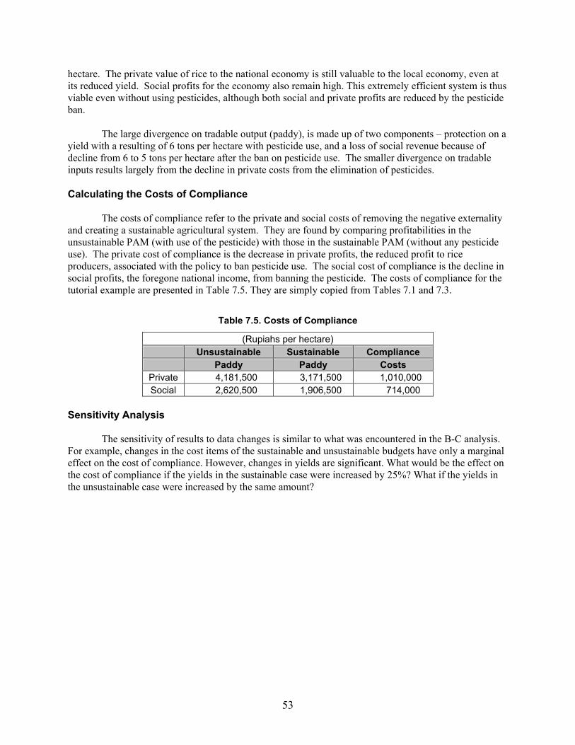
hectare. The private value of rice to the national economy is still valuable to the local economy, even at its reduced yield. Social profits for the economy also remain high. This extremely efficient system is thus viable even without using pesticides, although both social and private profits are reduced by the pesticide ban. The large divergence on tradable output (paddy), is made up of two components – protection on a yield with a resulting of 6 tons per hectare with pesticide use, and a loss of social revenue because of decline from 6 to 5 tons per hectare after the ban on pesticide use. The smaller divergence on tradable inputs results largely from the decline in private costs from the elimination of pesticides. Calculating the Costs of Compliance The costs of compliance refer to the private and social costs of removing the negative externality and creating a sustainable agricultural system. They are found by comparing profitabilities in the unsustainable PAM (with use of the pesticide) with those in the sustainable PAM (without any pesticide use). The private cost of compliance is the decrease in private profits, the reduced profit to rice producers, associated with the policy to ban pesticide use. The social cost of compliance is the decline in social profits, the foregone national income, from banning the pesticide. The costs of compliance for the tutorial example are presented in Table 7.5. They are simply copied from Tables 7.1 and 7.3.

Table 7.5. Costs of Compliance

(Rupiahs per hectare) Unsustainable Sustainable Compliance Paddy Paddy Costs

Private 4,181,500 3,171,500 1,010,000 Social 2,620,500 1,906,500 714,000

Sensitivity Analysis The sensitivity of results to data changes is similar to what was encountered in the B-C analysis. For example, changes in the cost items of the sustainable and unsustainable budgets have only a marginal effect on the cost of compliance. However, changes in yields are significant. What would be the effect on the cost of compliance if the yields in the sustainable case were increased by 25%? What if the yields in the unsustainable case were increased by the same amount?

53

Chapter 1: A Framework for Agricultural Policy Analysis · Sjaiful Bhari June 2003 . ... Profits,...

Documents

Transcript of Chapter 1: A Framework for Agricultural Policy Analysis · Sjaiful Bhari June 2003 . ... Profits,...