Chapitre1
24
Azzeddine Soula¨ ımani M´ ecanique des fluides avanc´ ee SYS 860 Notes de cours 21 septembre 2006 ´ Ecole de technologie sup´ erieure Montr´ eal
-
Upload
abdou-diga -
Category
Technology
-
view
10 -
download
1
Transcript of Chapitre1

Azzeddine Soulaımani
Mecanique des fluides avanceeSYS 860
Notes de cours
21 septembre 2006
Ecole de technologie superieure
Montreal


1
Introduction
In fluid mechanics analysis the fluid is considered as a continuum material. Any infinitesimalvolume in space contains a large number of molecules in mutual interactions and only globaleffects such as pressure, temperature or velocity are analyzed. In the sequel, a fluid particlerefers to such an infinitesimal volume of fluid with a measurable mass and containing a largenumber of molecules.
1.1 Fluid particle kinematics
Fluid kinematics is the study of the particles motion without considering the forces thatcause the motion. It describes the time evolution of particles properties (position, velocity,acceleration, density, pressure, temperature, etc) during the motion as function of time andspace position.
1.1.1 Particle position vector
Consider a Cartesian reference system with origin O and an orthonormal basis (i1, i2, i3).For any fluid particle, the vector position is denoted by x(t) and is function of time t :
x(t) = x1(t)i1 + x2(t)i2 + x3(t)i3 (1.1)
with x1(t), x2(t), x3(t) are the position coordinates.In the following we will use the so-called Einstein’s notation convention, i.e. when an index
is repeated in a mathematical expression that means a summation over the repeated index.For example, equation (1.1) can be rewritten in a more compact form as
x(t) = x1(t)i1 + x2(t)i2 + x3(t)i3 =∑
k
xkik ≡ xkik.

2 1 Introduction
1.1.2 Particle velocity and acceleration vectors
Consider a fluid particle at time t. During a small time duration ∆t, the vector positionbecomes x(t + ∆t) and the displacement vector of the particle is
∆x = x(t + ∆t)− x(t).
x3
x1
O
i1x2
Particle at time t + ∆t
x(t + ∆t)
x(t)
Particle at time t
i3
i2
Vector displacement after ∆t∆x = x(t + ∆t)− x(t)
Fig. 1.1. Particle position vector
The particle velocity vector is defined as the rate of change of the vector position :
u(t) = lim∆t→0
∆x∆t
=dxdt
(1.2)
The particle acceleration vector is defined as the rate of change of the velocity vector :
a(t) = lim∆t→0
∆u∆t
=dudt
=d2xdt2
(1.3)
1.1.3 Lagrangian and Eulerian Kinematic Descriptions
To define the velocity and acceleration vectors, we need actually to specify or to identifywhich particle is under study. One convenient way is to label each particle by its position ξ at acertain initial time t0. Then the motion of the whole fluid can be described by two independent

1.1 Fluid particle kinematics 3
variables ξ and t. For a particle with label ξ, equation x = x(ξ, t) gives the particle trajectoryor patheline. The velocity and acceleration vectors are then given more precisely by
u(ξ, t) =[∂x(ξ, t)
∂t
]
ξ
, (1.4)
and
a(ξ, t) =[∂u(ξ, t)
∂t
]
ξ
. (1.5)
The use of the independent variables ξ and t is called the Lagrangian or the materialdescription. Another description very often used in fluid kinematics is to use as independentvariables x and t. That is, we are interested to describe the motion of the particle which passesat a fixed position x in space and at the time instant t. This description is called the Euleriankinematic description and is very often used in Fluid Mechanics. Solving equation ξ = ξ(x, t)gives the labels of all particles that occupied the fixed position x. The velocity and accelerationvectors can now be described as functions of x and t,
u(x, t) = u(x(ξ, t), t) (1.6)
and
a(x, t) = a(x(ξ, t), t) (1.7)
1.1.4 Material derivative
In the following we will obtain the derivative with respect to time when using the Euleriandescription. Consider first a scalar material property θ(x, t) such as pressure or temperature.The rate of change of this property felt by the particle labeled by ξ as it moves is defined by
Dθ
Dt≡
[dθ(x(ξ, t), t)
dt
]
ξ
. (1.8)
Using the differentiation chain rule, equation (1.8) is developed into
Dθ
Dt=
[∂θ(x, t)
∂t
]
t
+∂θ
∂x1
∂x1(ξ, t)∂t
+∂θ
∂x2
∂x2(ξ, t)∂t
+∂θ
∂x3
∂x3(ξ, t)∂t
. (1.9)
The first term on the right hand side of equation (1.9) is the rate of change of the propertyθ at the fixed position x. This term is called the local derivative, and is non zero when, forinstance, the boundary conditions of the fluid domain change in time. The other terms in (1.9)give the rate of change when the particle moves from x to x + ∆x. It is called the convective
derivative. In fact the terms∂xk
∂tare the velocity components uk which convect or transport
the material property. The convective derivative is non zero when, for instance, there is a
variation in the domain geometry that causes a spatial variation∂θ
∂xk. An illustration of the

4 1 Introduction
Lateral boundary heated in a non uniform manner
Incomming flow with
temperature
time varying
Temperature measurement
A(x1) x1
x1 = 0
u1(x1, t)
Θ(0, t)
Θ(x1, t)
x1
Fig. 1.2. An illustration for temperature material derivative measurement
local and convective rate of change is given in figure (1.2). A fluid flows in a duct with a variablecross section A(x). For simplicity, we assume that the flow is unidirectional with velocity u1.The incoming fluid has a time dependent temperature θ(0, t), that is the boundary conditionat the inlet is time varying. A thermometer is placed at a fixed position x1. By taking twosuccessive temperature observations θ(x1, t) and θ(x1, t + ∆t) in a small time interval ∆t wecan indirectly measure the local temperature derivative, i.e.
[∂θ(x1, t)
∂t
]
x1
≈ θ(x1, t + ∆t)− θ(x1, t)∆t
.
Another thermometer is placed at a close position x1 + ∆x1, so that the rate of temperaturechange observed by the particle in its travel of the distance ∆x1 (with ∆x1 ≈ u1(x1, t)∆t) canbe approximated by
u1(x1, t)θ(x1 + ∆x1, t)− θ(x1, t)
∆x1.
The temperature gradient can be caused by heating the lateral boundary in a nonuniformmanner. Thus the material derivative of the particle passing at position x1 at time t can beindirectly measured without actually moving the thermometer with this particle. Therefore,only the flow field u1(x1, t) and the temperature field θ(x1, t) have to be measured at differenttime intervals to be able to compute the material derivative.
Using indicial notation, the material derivative can be rewritten as
Dθ
Dt(x, t) =
∂θ(x, t)∂t
+ uk∂θ
∂xk(1.10)
Equation (1.10) can also be written in a matrix form as
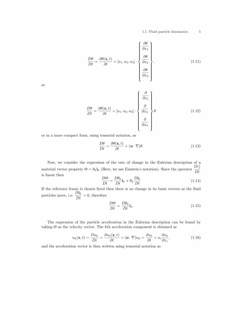
1.1 Fluid particle kinematics 5
Dθ
Dt=
∂θ(x, t)∂t
+ [u1, u2, u3] ·
∂θ
∂x1
∂θ
∂x2
∂θ
∂x3
, (1.11)
or
Dθ
Dt=
∂θ(x, t)∂t
+ [u1, u2, u3] ·
∂
∂x1
∂
∂x2
∂
∂x3
θ (1.12)
or in a more compact form, using tensorial notation, as
Dθ
Dt=
∂θ(x, t)∂t
+ (u · ∇)θ. (1.13)
Now, we consider the expression of the rate of change in the Eulerian description of a
material vector property Θ = θkik (Here, we use Eisntein’s notation). Since the operatorD()Dt
is linear thenDΘ
Dt=
Dθk
Dtik + θk
DikDt
(1.14)
If the reference frame is chosen fixed then there is no change in its basis vectors as the fluid
particles move, i.e.DikDt
= 0, therefore
DΘ
Dt=
Dθk
Dtik. (1.15)
The expression of the particle acceleration in the Eulerian description can be found bytaking Θ as the velocity vector. The kth acceleration component is obtained as
ak(x, t) =Duk
Dt=
∂uk(x, t)∂t
+ (u · ∇)uk =∂uk
∂t+ ui
∂uk
∂xi, (1.16)
and the acceleration vector is then written using tensorial notation as

6 1 Introduction
a(x, t) =Du(x, t)
Dt=
∂u(x, t)∂t
+ (u · ∇)u. (1.17)
The first term on the right hand side of equation (1.17) represents the local acceleration. Thelast term represents the convective acceleration which is nonlinear since a product of u by itsgradient appears.
1.1.5 Pathlines and streamlines
The pathline is defined by the successive positions occupied by the particle ξ. If the ve-locity field u(x, t) is known then the pathline can be obtained by solving for x the followingdifferential equation :
dxdt
= u(x, t). (1.18)
The streamlines are defined as the lines tangent to the velocity vector. Any vector displacement
Streamline
Particule position at time
Pathline
u(x, t)
t
x(ξ, t)
Fig. 1.3. Figure 1.3. Pathline and streamline
dx along the streamlines is parallel to the velocity vector :
dx× u = 0, (1.19)
which can be developed in the orthonnormal basis as∣∣∣∣∣∣
dx1 u1 i1dx2 u2 i2dx3 u3 i3
∣∣∣∣∣∣= (u3dx2 − u2dx3)i1 + (u1dx3 − u3dx1)i2 + (u2dx1 − u1dx2)i3 = 0 (1.20)
This leads to solving a set of differential equations :
dx1
u1=
dx2
u2=
dx3
u3. (1.21)
Example 1.1 : Steady flow in a convergent duct
An incompressible fluid flows in a duct having a convergent cross section A(x1) =A0
1 +x1
l
,
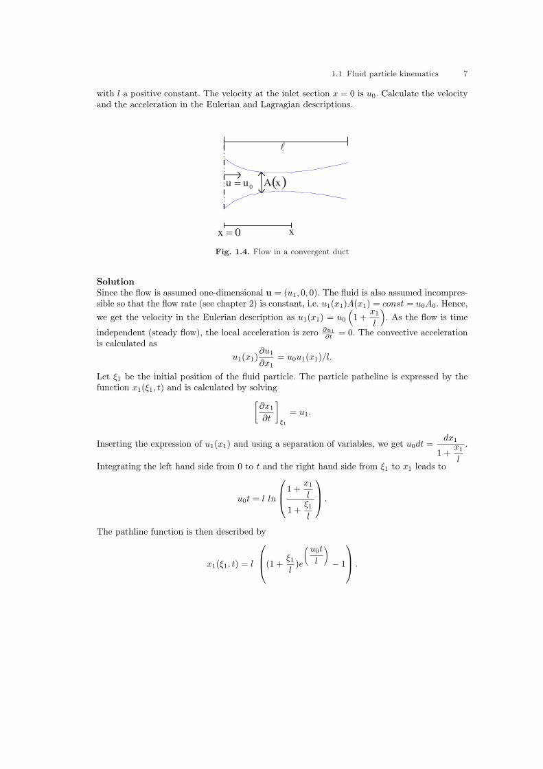
1.1 Fluid particle kinematics 7
with l a positive constant. The velocity at the inlet section x = 0 is u0. Calculate the velocityand the acceleration in the Eulerian and Lagragian descriptions.
xA0
uu
0x x
Fig. 1.4. Flow in a convergent duct
SolutionSince the flow is assumed one-dimensional u = (u1, 0, 0). The fluid is also assumed incompres-sible so that the flow rate (see chapter 2) is constant, i.e. u1(x1)A(x1) = const = u0A0. Hence,we get the velocity in the Eulerian description as u1(x1) = u0
(1 +
x1
l
). As the flow is time
independent (steady flow), the local acceleration is zero ∂u1∂t = 0. The convective acceleration
is calculated asu1(x1)
∂u1
∂x1= u0u1(x1)/l.
Let ξ1 be the initial position of the fluid particle. The particle patheline is expressed by thefunction x1(ξ1, t) and is calculated by solving
[∂x1
∂t
]
ξ1
= u1.
Inserting the expression of u1(x1) and using a separation of variables, we get u0dt =dx1
1 +x1
l
.
Integrating the left hand side from 0 to t and the right hand side from ξ1 to x1 leads to
u0t = l ln
1 +x1
l
1 +ξ1
l
.
The pathline function is then described by
x1(ξ1, t) = l
(1 +
ξ1
l)e
(u0t
l
)
− 1
.

8 1 Introduction
On the other hand, given a fixed position x1 we can also obtain the Lagrangian variableξ1(x1, t) of the particles passing by x1. Hence,
ξ1(x1, t) = l
(1 +
x1
l)e
(−u0t
l) − 1
.
The velocity in the Lagrangian description is defined by u1(ξ, t) =[∂x1
∂t
]
ξ1
and thus by a
simple differentiation we obtain
u1(ξ1, t) = u0(1 +ξ1
l)e( u0t
l).
Since (1 +ξ1
l)e
(u0t
l)= 1 +
x1
lwe can verify that the we obtain the same result for the velocity
in the Lagranian and Eulerian descriptions.The Lagrangian description of the acceleration is
a1(ξ1, t) =[∂u1
∂t
]
ξ1
=u2
0
l(1 +
ξ1
l)e( u0t
l).
Example 1.2 : Unsteady flow in a convergent ductRepeat example (1.1) with a time dependent boundary condition u1(0, t) = u0(t) = Ue−αt
with U and α positive constants.
SolutionThe velocity field is time dependent because of the time varying nature of the inflow. As before,invoking the principle of mass conservation for an incompressible fluid the velocity at anyspace position is obtained u1(x1, t) = u0(t)
(1 +
x1
l
). The local and convective accelerations
are respectively∂u1(x, t)
∂t= −αUe−αt
(1 +
x1
l
)and u0(t)u1(x1, t)/l.
Again, we obtain the particle pathline by solving the differential equation[∂x1
∂t
]
ξ1
= u1(x1, t).
Using the method of separation of variables, we obtain the pathline equation
x1(t) = l
((1 +
ξ1
l)ef(t) − 1
),
with
f(t) = −U
lα
(e(−αt) − 1
)= ln
1 +x1
l
1 +ξ1
l
.

1.1 Fluid particle kinematics 9
The Lagrangian variable at time t corresponding to a fixed spatial position is
ξ1(x1, t) = l((1 +
x1
l)e−f(t) − 1
).
The velocity in the Lagrangian description is u1(ξ, t) =[∂x1
∂t
]
ξ1
= lf ′(t)(1 + 1
l)ef(t), which
can be verified to be equal to Ue−αt(1 +x1
l) = u1(x1, t). When the velocity u1(ξ, t) is differen-
tiated with respect to time this gives the acceleration a1(ξ, t) in the Lagrangian description.Example 1.3 : Steady two-dimensional flow close to a stagnation pointThe motion of a fluid is described by its velocity field given in the Eulerian description by :
u = α(x1,−x2)
with α a positive constant.a) Determine the velocity field and acceleration in the Lagrangian and Eulerian descriptions.Find the pathline equation of a particle which occupied position ξ = (ξ1, ξ2) at time 0.b) Find the streamline equation of a particle which occupied position x at time t.Solutiona) The velocity components in the Eulerian description are : u1 = αx1 and u2 = −αx2. As aresult, the acceleration components are determined using equation (1.16), a1(x, t) = α2x1 anda2(x, t) = α2x2.The pathline differential equations are :
ui(x, t) =[∂xi
∂t
]
ξ
.
By integration, we obtain the pathline equations :
x1(ξ, t) = ξ1 exp(αt)
andx2(ξ, t) = ξ2 exp(−αt).
In these equations t represents the curve parameter of the pathline, and ξi are the paramete-rized families. By eliminating the curve parameter t,
t = (1α
) ln(x1
ξ1) = −(
1α
) ln(x2
ξ2)
we obtain the explicit form of the pathline equation
x2 =ξ1ξ2
x1,
which defines a family of hyperboles.The velocity components in the Lagrangian description are u1(ξ, t) = αξ1 exp(αt) andu2(ξ, t) = −αξ2 exp(−αt). The acceleration components in the Lagrangian description are
10 1 Introduction
a1(ξ, t) = α2ξ1 exp(αt) and a2(ξ, t) = α2ξ2 exp(−αt).b)The streamline differential equations are given by equation (1.21) which leads in the case ofa two-dimensional flow to solving the differential equation
∂x2
∂x1=
u2
u1.
Inserting the expression of the velocity components we obtain
∂x2
∂x1= −x2
x1.
And by integration, we obtain x2 = C1C21x1
with C1 and C2 two constants of integration.Therefore, the streamlines define families of hyperboles identical to those defined by the path-lines.
Example 1.4 : Material derivative in cylindrical coordinates
a) Develop the divergence ∇ · v of the vector v using cylindrical coordinates (r, θ, z) and thepolar orthonormal basis (er, eθ, ez).b) Derive the material derivative for a scalar function T in cylindrical coordinates.c) Derive the material derivative for a vector function v in cylindrical coordinates.
Solutiona)Recall that the Cartesian basis vectors are related to the basis vectors (er, eθ, ez) by :
i1 = cos θ er − sin θ eθ,
i2 = sin θ er + cos θ eθ,
i3 = ez.
The velocity in the cylindrical system is :
u = urer + uθeθ + uzez
The unit vectors er and eθ vary with the angle. We have the following relations∂er
∂θ= eθ
and∂eθ
∂θ= −er.
The gradient operator in cylindrical polar coordinates can be verified as (do it as an exer-cise) :
∇ = er∂
∂r+ eθ
1r
∂
∂θ+ ez
∂
∂z.
Let consider a vector v = vrer + vθeθ + vzez. The divergence is defined as the scalar productof the gradient vector with the vector v. Thus,
∇·v = (er∂
∂r+eθ
1r
∂
∂θ+ez
∂
∂z)·(vrer+vθeθ+vzez) =
∂vr
∂r+eθ
1r·(
vr∂er
∂θ+
∂vθ
∂θeθ + vθ
∂eθ
∂θ
)+
∂vz
∂z

1.1 Fluid particle kinematics 11
=⇒∇ · v =
∂vr
∂r+
vr
r+
1r
∂vθ
∂θ+
∂vz
∂z.
b)The material derivative of a function T (r, θ, z, t) is obtained as :
DT
Dt=
∂T
∂t+
∂T
∂r
∂r
∂t+
∂T
∂θ
∂θ
∂t+
∂T
∂z
∂z
∂t.
The velocity components in the polar system are ur =∂r
∂t, uθ = r
∂θ
∂tand uz =
∂z
∂t. Then, the
material derivative in cylindrical coordinates is :
DT
Dt=
∂T
∂t+ ur
∂T
∂r+
uθ
r
∂T
∂θ+ uz
∂T
∂z.
It can be verified that the convection operator is given in cylindrical coordinates by
u · ∇ = (urer + uθeθ + uzez) · (er∂
∂r+ eθ
1r
∂
∂θ+ ez
∂
∂z.) = ur
∂
∂r+
uθ
r
∂
∂θ+ uz
∂T
∂z.
Therefore, the material derivative can be written as
DT
Dt=
∂T
∂t+ (u · ∇)T
which is the same tensorial expression as in the Cartesian coordinates system.
c)The material derivative for a vector field v(r, θ, z, t) = vrer + vθeθ + vzez is obtained as
DvDt
=Dvr
Dter + vr
Der
Dt+
Dvθ
Dteθ + vθ
Deθ
Dt+
Dvz
Dtez + vz
Dez
Dt.
Noting thatDer
Dt=
∂er
∂θ
∂θ
∂t=
uθ
reθ
Deθ
Dt=
∂eθ
∂θ
∂θ
∂t= −uθ
rer
thenDvDt
=(
Dvr
Dt− vθuθ
r
)er +
(Dvθ
Dt+
vruθ
r
)eθ +
Dvz
Dtez.
If we replace v by the velocity then the acceleration a has in cylindrical coordinates systemthe components :
ar =Dur
Dt− uθ
2
r=
∂ur
∂t+ (u · ∇)ur − uθ
2
r,
aθ =Duθ
Dt+
uθur
r=
∂uθ
∂t+ (u · ∇)uθ +
uθur
r

12 1 Introduction
andaz =
Duz
Dt=
∂uz
∂t+ (u · ∇)uz.
Example 1.5 : Material derivative in natural coordinates
a) The unit tangent vector to the pathline is :
−→τ =dxdx
and its unit normal vector in the two dimensional space is
n = Rd−→τds
with s the coordinate in the direction of −→τ and n is the coordinate in the direction of n. (−→τ ,n)define a local orthonormal basis. Derive the acceleration components on this basis.
SolutionThe velocity components on the local basis are uτ and un = 0. The material derivative of thevelocity is
DuDt
=Du
Dt−→τ + u
D−→τdt
Now we develop the following terms :
Du(s, n, t)Dt
=∂u
∂t+ u
∂u
∂s+ un
∂u
∂n,
andD−→τDt
=u
Rn.
Since un = 0 and ∂un
∂s = 0 thenDu
Dt=
∂u
∂t+ u
∂u
∂s.
It follows that the acceleration in the local basis is
DuDt
= (∂u
∂t+ u
∂u
∂s)−→τ +
u2
Rn.
1.2 Velocity gradients and Deformations
1.2.1 Linear Deformations
The simplest motion that a fluid particle can undergo is translation. Consider a small fluidelement with a brick shape. The edges lengths are infinitesimal and are denoted by δx1, δx2
and δx3. The original volume is δϑ = δx1δx2δx3.

1.2 Velocity gradients and Deformations 13
C’CB
A A’O
δx2
u1
u1 +∂u1
∂x1δx1
δx1
∂u1
∂x1δx1
u1 +∂u1
∂x1δx1
u1
∂u1
∂x1δx1
Fig. 1.5. Linear deformation for a fluid element
Let us first analyze the effect of a translation motion in the i1 direction.Particularly, we are interested to study the deformations as the fluid element moves during
a small time interval δt. The edge OB is translated into O′B′ by the velocity component u1 and
the edge AC is translated into A′C ′ by the velocity component u1(x1 + δx1) ≈ u1 +∂u1
∂x1δx1.
Because of this velocity difference, edges’ OA and BC lengths are changed by∂u1
∂x1δx1δt.
Therefore, the particle deforms and its volume changes by δϑ =∂u1
∂x1δx1δx2δx3δt. The rate at
which the original volume is changing per unit volume is
limδt→0
1δϑ
δϑ
δt= lim
δt→0
∂u1
∂x1δx1δx2δx3δt
δx1δx2δx3δt=
∂u1
∂x1(1.22)
When there is no velocity gradient, the fluid element undergoes a pure translation withoutdeformation.The total rate of change of the fluid particle volume per unit volume for a three-dimensionaltranslation can be readily obtained
limδt→0
1δϑ
δϑ
δt=
∂u1
∂x1+
∂u2
∂x2+
∂u3
∂x3=
∂uk
∂xk= ∇.u = div(u) (1.23)
The velocity gradient components∂uk
∂xkare responsible for the volumetric dilatation. The
other components of the velocity gradient (i.e.,∂ui
∂xkfor i 6= k) cause rotations and angular
deformations. By definition an incompressible fluid has no volumetric dilation therefore in thiscase div(u) = 0.
1.2.2 Angular deformation
For illustration, we will consider motion in the x1−x2 plane. The velocity gradient compo-nents that cause rotation and angular deformation are illustrated in figure ?. During a small

14 1 Introduction
O A
CB
δx2
δx1
u2 +∂u2
∂x1δx1
u1 +∂u1
∂x2δx2
u1
u2
Fig. 1.6. Velocity components responsible for angular rotation and deformation
O
CB
C’
B’
A’
A
δx2
δx1U1
U2
(∂u2
∂x1δx1
)δtδα
δβ
(∂u1
∂x2δx2
)δt
Fig. 1.7. Angular rotation and deformation for a fluid element
time interval δt, edges OA and OB will rotate to O′A′ and O′B′ by angles δα and δβ. Apositive rotation is by convention counterclockwise. The angular velocity of edge OA is
ω0A = limδt→0
δα
δt(1.24)
For small angles :
δα ≈ tan(δα) =
∂u2
∂x1δx1δt
δx1=
∂u2
∂x1δt (1.25)
and (1.24) becomes
ω0A = limδt→0
δα
δt=
∂u2
∂x1(1.26)
Similarly, the angular velocity of edge OB is
ω0B = − limδt→0
δβ
δt= −∂u1
∂x2(1.27)
The rotation of the fluid element about the x3 axis is defined as the average of the angularvelocities ω0A and ω0B , it follows that

1.2 Velocity gradients and Deformations 15
ω3 =ω0A + ω0B
2=
12
(∂u2
∂x1− ∂u1
∂x2
)(1.28)
The angular velocities about the other axis ω1 and ω2 can be obtained using a similar analysis,and they are respectively
ω1 =12
(∂u3
∂x2− ∂u2
∂x3
)and ω2 =
12
(∂u1
∂x3− ∂u3
∂x1
)(1.29)
The three angular velocities ω1, ω2 and ω3 define the rotation vector ω as
ω = ω1i1 + ω2i2 + ω3i3 (1.30)
This vector represents actually half of the curl of the velocity vector,
ω =12curl(u) (1.31)
since by definition of the vector operator ∇× u
curl(u = ∇× u =
∣∣∣∣∣∣∣
i1 i2 i3∂
∂x1
∂
∂x2
∂
∂x3u1 u2 u3
∣∣∣∣∣∣∣= 2ω (1.32)
To eliminate the factor 1/2, the vorticity is defined as twice the rotation vector
ζ = 2ω = ∇× u. (1.33)
It can be concluded at this point that the divergence of the velocity represents the lineardeformations while the curl represents rotations. On the other hand, there are also angulardeformations associated with the cross derivatives as can be observed from figure (1.7). Thechange in the original right angle formed by the edges OA and OB is a shearing deformation
δγ12 = δα + δβ
where it is considered positive if the original right angle is decreased. The rate of angulardeformation (or shearing strain) is
γ12 = limδt→0
δγ12
δt= lim
δt→0
∂u2
∂x1δt +
∂u1
∂x2δt
δt
=
∂u2
∂x1+
∂u1
∂x2(1.34)
If∂u2
∂x1= −∂u1
∂x2, the angular deformation is zero and this corresponds to a pure rotation. Using
a similar analysis, the other two rate shearing strains in the planes x1 − x3 and x2 − x3 canbe obtained and are respectively
γ13 =∂u3
∂x1+
∂u1
∂x3and γ23 =
∂u3
∂x2+
∂u2
∂x3. (1.35)

16 1 Introduction
1.2.3 Tensors in Fluid Kinematics
It follows from the previous section that the spatial derivatives of the velocity field definethree different tensors :
¤ The velocity gradient :
F =
∂u1
∂x1
∂u1
∂x2
∂u1
∂x3∂u2
∂x1
∂u2
∂x2
∂u2
∂x3∂u3
∂x1
∂u3
∂x2
∂u3
∂x3
= ∇uT . (1.36)
¤ The rate of strain (or rate of deformation) :
D =
ε11 ε12 ε13ε21 ε22 ε23ε31 ε32 ε33
=
F + FT
2=
(∇u + (∇u)T )2
(1.37)
where
εkl =12(∂uk
∂xl+
∂ul
∂xk) (1.38)
– The strain tensor is symmetric and detailed more clearly as follows :
D =
∂u1
∂x1
12(∂u1
∂x2+
∂u2
∂x1)
12(∂u1
∂x3+
∂u3
∂x1)
12(∂u2
∂x1+
∂u1
∂x2)
∂u2
∂x2
12(∂u2
∂x3+
∂u3
∂x2)
12(∂u3
∂x1+
∂u1
∂x3)
12(∂u3
∂x2+
∂u2
∂x3)
∂u3
∂x3
(1.39)
– εkk =∂uk
∂xk= tr(D) is the volumetric deformation.
– 2εkl = γkl is the rate of angular deformation.
¤ The spin tensor :
S = F−D =F− FT
2(1.40)
is the antisymmetric part of the velocity gradient and is detailed as follows

1.2 Velocity gradients and Deformations 17
S =
012(∂u1
∂x2− ∂u2
∂x1)
12(∂u1
∂x3− ∂u3
∂x1)
12(∂u2
∂x1− ∂u1
∂x2) 0
12(∂u2
∂x3− ∂u3
∂x2)
12(∂u3
∂x1− ∂u1
∂x3)
12(∂u3
∂x2− ∂u2
∂x3) 0
=
0 −ω3 ω2
ω3 0 −ω1
−ω2 ω1 0
(1.41)
– Using index notation, the components of the above tensors can be written in a compactform as follows :
Fij =∂ui
∂xj(1.42)
Dij =Fij + Fji
2=
12(∂ui
∂xj+
∂uj
∂xi) (1.43)
Sij =Fij − Fji
2=
12(∂ui
∂xj− ∂uj
∂xi) (1.44)
Remark : The velocity field in the vicinity of a fluid particle at position x can be completelydescribed if the velocity gradient tensor is known. Using Taylor’s expansion, the velocity at aclose position x + dx is approximated at the first order by
u(x + dx, t) = u(x, t) +∇uT · dx (1.45)
since the velocity gradient tensor is decomposed into a symmetric and an antisymmetric partthen
u(x + dx, t) = u(x, t) + S · dx + D · dx (1.46)
Furthermore, it can be easily verified that
S · dx = ω × dx
The motion of a fluid element located at position x with length dx and aligned along vectordx can be decomposed into a pure translation by velocity u(x, t), a pure rotation at velocityω, and deformations (linear and angular) at a rate D · dx.
Example 1.6 : Deformations for a shearing flow
Consider a simple two dimensional flow whose velocity is given by
u1 = ax2
andu2 = 0.
18 1 Introduction
Derive all related tensors and give an interpretation for the fluid motion.
SolutionThe velocity gradient tensor is readily obtained
∇uT =[
0 a0 0
].
Its symmetric and antisymmetric parts are respectively
D =12
[0 aa 0
]
and
S =12
[0 a−a 0
].
The rotation vector has one non zero component
ω3 = −a
2,
hence the flow is rotational. It can be seen that a square element translates horizontally by avelocity u1 while its vertical edges rotate clockwise by an angle
dβ = adt
so that its rate of rotation is a. The volume of the fluid element is unchanged, but the diagonalline will rotate clockwise at the rate − 1
2a. On the other hand, the angle originally at π2 is
reduced by an angle adt, which shows that the fluid element is sheared at the rate γ = a.
Example 1.7 : Deformations for a stagnation flow
Consider a simple two dimensional flow whose velocity is given by
u1 = ax1
andu2 = −ax2.
Derive all related tensors and give an interpretation for the fluid motion.
SolutionThe velocity gradient tensor is readily obtained
∇uT =[
a 00 −a
].
Since it is a symmetric tensor then its symmetric and antisymmetric parts are respectively
1.2 Velocity gradients and Deformations 19
D = ∇uT
andS = 0.
Since S = 0, the flow is irrotational. The sum of the diagonal coefficients of the deformationtensor is zero, therefore the volumetric dilatation is zero (in other words the flow is incompres-sible). From figure ( ) we can see that the fluid element can be decomposed into a translationmotion by the velocity vector u and a relative motion which causes deformations whose velo-city is (∂u1
∂x1dx1,
∂u2∂x2
dx2) = (adx1,−adx2). The angle variations dβ and dα are zero. This showsthat the fluid elements does not rotate and has no shearing. It has only linear deformations(for a positive value of a, it corresponds to an expansion in the horizontal direction and acompression in the vertical one).
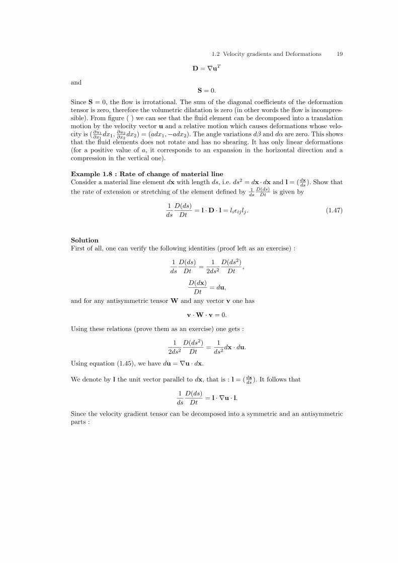
Example 1.8 : Rate of change of material lineConsider a material line element dx with length ds, i.e. ds2 = dx · dx and l = (dx
ds ). Show thatthe rate of extension or stretching of the element defined by 1
dsD(ds)
Dt is given by
1ds
D(ds)Dt
= l ·D · l = liεij lj . (1.47)
SolutionFirst of all, one can verify the following identities (proof left as an exercise) :
1ds
D(ds)Dt
=1
2ds2
D(ds2)Dt
,
D(dx)Dt
= du,
and for any antisymmetric tensor W and any vector v one has
v ·W · v = 0.
Using these relations (prove them as an exercise) one gets :
12ds2
D(ds2)Dt
=1
ds2dx · du.
Using equation (1.45), we have du = ∇u · dx.
We denote by l the unit vector parallel to dx, that is : l = (dxds ). It follows that
1ds
D(ds)Dt
= l · ∇u · l.
Since the velocity gradient tensor can be decomposed into a symmetric and an antisymmetricparts :

20 1 Introduction
1ds
D(ds)Dt
= l · (D + S) · l.Since the spin tensor S is antisymmetric, the product l · S · l is zero. We can conclude that,
1ds
D(ds)Dt
= l ·D · l = liεij lj . (1.48)
Equation (1.48) gives an interpretation of the coefficients of the strain tensor. If the materialelement is parallel to a basis vector, for instance i1, then 1
dsD(ds)
Dt = l ·D · l = ε11. Therefore,the diagonal elements of D represents the stretching of the material element parallel to theaxes.
Example 1.9 : Rate of change of the angle between material vectorsConsider two material line elements a and b. Initially these vectors make a right angle. Showthat the rate of change of the angle is :
D(θ)Dt θ= π
2
= −2a ·D · b
1.3 Problems
1.1. Measurements of a one dimensional velocity field give the following results :
Time x=0m x=10m x=20mt=0s v=0m/s v=0m/s v=0m/st=1s v=1m/s v=1.2m/s v=1.4m/st=2s v=1.7m/s v=1.8m/s v=1.9m/st=3s v=2.1m/s v=2.15m/s v=2.2m/sCalculate the acceleration at t = 1s and x = 10m .
1.2. Consider the velocity components : u = x2 − y2 et v = −2xy. Calculate the divergenceand vorticity.
1.3. Consider the velocity field whose components are : u1 = a(x1 + x2)u2 = a(x1 − x2)u3 = w with a, w are constants. Determine the divergence , vorticity and the pathlines.
1.4. Consider the velocity field :
u1 = bx2
u2 = bx1
u3 = 0
et
u1 = −bx2
u2 = bx1
u3 = 0
Is the flow incompressible ?. Is it rotational ?.
1.5. Consider the velocity field v=(u,υ) with u = cx + 2ωy + y0 et υ = cy + υ0. Compute thevorticity and the strain tensor.

1.3 Problems 21
1.6. Consider the velocity field u = ax2 + by and v = −2axy + ct. Is the flow incompressible ?Determine the streamlines.
1.7. Verify the following relations :– a) div(φv) = φdiv(v) + vgrad(φ)– b) div(u× v) = v.curl(u)− u.curl(v)– c) (τ : ∇v) = ∇(τv)− v∇τ with A : B =
∑i
∑j AijBij
1.8. – Find the expanded forms of the quantities :
(u.∇)u
(∇u).u
σ.u
div((∇u).u)
– Show that the magnitude of the vorticity vector is :
|ζ|2 =∂ui
∂xj(∂ui
∂xj− ∂uj
∂xi)
1.9. Show that the vorticity vector in cylindrical coordinates is given by :
curlu = ∇× u = (1r
∂uz
∂θ− ∂uθ
∂r)er + (
∂ur
∂z− ∂uz
∂r)eθ + (
1r(∂(ruθ)
∂r− ∂ur
∂θ))ez
Calculate the vorticity for the following velocity field (fluid in solid rotation) : u = uθ(r)eθ
where uθ(r) = ωr