Chap00 1b Performance Measurement

© 2011 Pearson Education, Inc. publishing as Prentice Hall

Break-Even Analysis

Technique for evaluating process and equipment alternatives

Objective is to find the point in dollars and units at which cost equals revenue

Requires estimation of fixed costs, variable costs, and revenue


Break-Even Analysis Fixed costs are costs that continue even if

no units are produced Depreciation, taxes, debt, mortgage

payments Variable costs are costs that vary with the

volume of units produced Labor, materials, portion of utilities Contribution is the difference between

selling price and variable cost


Break-Even Analysis

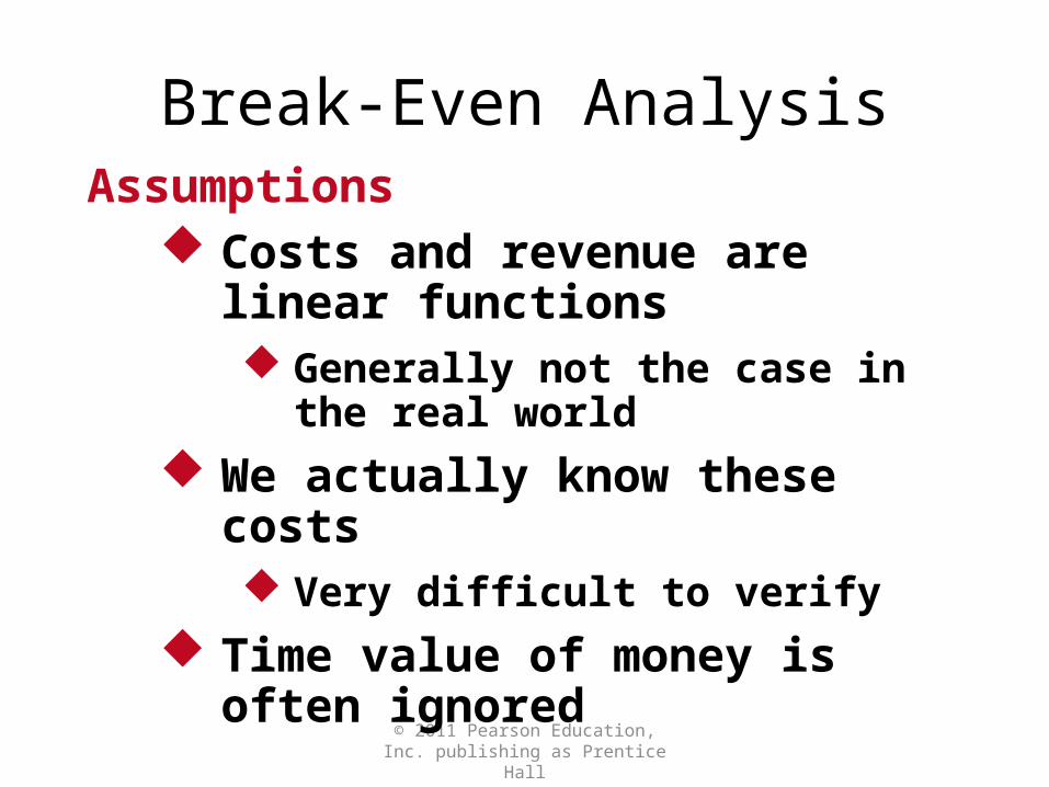
Costs and revenue are linear functions Generally not the case in the real

world We actually know these costs

Very difficult to verify Time value of money is often

ignored

Assumptions


Profit corridor

Loss

corridor

Break-Even AnalysisTotal revenue line

Total cost line

Variable cost

Fixed cost

Break-even pointTotal cost = Total revenue

–

900 –

800 –

700 –

600 –

500 –

400 –

300 –

200 –

100 –

–| | | | | | | | | | | |

0 100 200 300 400 500 600 700 800 900 1000 1100

Cost

in d

olla

rs

Volume (units per period)Figure S7.5


Break-Even Analysis

BEPx =break-even point in unitsBEP$ =break-even point in dollarsP = price per unit (after all discounts)

x = number of units producedTR = total revenue = PxF = fixed costsV = variable cost per unitTC = total costs = F + Vx

TR = TCor

Px = F + Vx

Break-even point occurs when

BEPx =F

P - V


Break-Even Analysis

BEPx =break-even point in unitsBEP$ =break-even point in dollarsP = price per unit (after all discounts)

x = number of units producedTR = total revenue = PxF = fixed costsV = variable cost per unitTC = total costs = F + Vx

BEP$ = BEPx P

= P

=

=

F(P - V)/P

FP - V

F1 - V/P

Profit = TR - TC= Px - (F + Vx)= Px - F - Vx= (P - V)x - F


Break-Even Example

Fixed costs = $10,000 Material = $.75/unitDirect labor = $1.50/unit Selling price = $4.00 per unit

BEP$ = F1 -(V/P)

$10,0001 - [(1.50 + .75)/(4.00)]


Break-Even Example

Fixed costs = $10,000 Material = $.75/unitDirect labor = $1.50/unit Selling price = $4.00 per unit

BEP$ = =F

1 -(V/P)$10,000

1 - [(1.50 + .75)/(4.00)]

= $10,000

.4375

BEPx = F

P - V$10,000

4.00 - (1.50 + .75)

= $22,857.14

= = 5,714


Break-Even Example

50,000 –

40,000 –

30,000 –

20,000 –

10,000 –

–| | | | | |

0 2,000 4,000 6,000 8,000 10,000

Dol

lars

Units

Fixed costs

Total costs

Revenue

Break-even point


Multiproduct Example

Annual ForecastedItem Price Cost Sales UnitsSandwich $5.00 $3.00 9,000Drink 1.50 .50 9,000Baked potato 2.00 1.00 7,000

Fixed costs = $3,000 per month





Sandwich $5.00 $3.00 .60 .40 $45,000 .621 .248Drinks 1.50 .50 .33 .67 13,500 .186 .125Baked 2.00 1.00 .50 .50 14,000 .193 .096 potato

$72,500 1.000 .469

Annual WeightedSelling Variable Forecasted % of Contribution

Item (i) Price (P) Cost (V) (V/P) 1 - (V/P) Sales $ Sales (col 5 x col 7)





Sandwich $5.00 $3.00 .60 .40 $45,000 .621 .248Drinks 1.50 .50 .33 .67 13,500 .186 .125Baked 2.00 1.00 .50 .50 14,000 .193 .096 potato

$72,500 1.000 .469

Annual WeightedSelling Variable Forecasted % of Contribution

Item (i) Price (P) Cost (V) (V/P) 1 - (V/P) Sales $ Sales (col 5 x col 7)

BEP$ =F

∑ 1 - x (Wi)Vi

Pi

= = $76,759$3,000 x 12

.469

Daily sales = = $246.02

$76,759312 days

.621 x $246.02$5.00 = 30.6 31

sandwichesper day


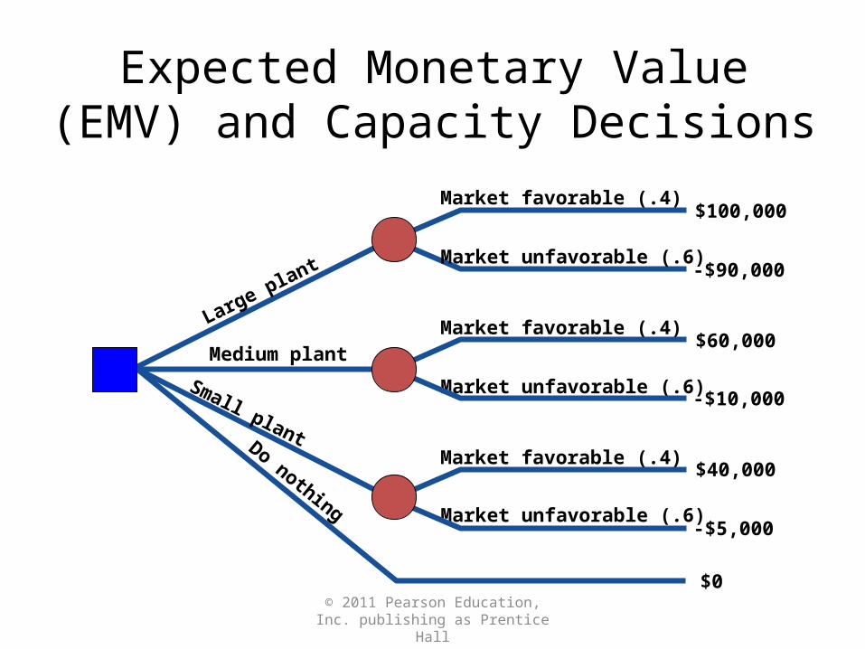
Expected Monetary Value (EMV) and Capacity Decisions

Determine states of nature Future demand Market favorability

Analyzed using decision trees Hospital supply company Four alternatives



-$90,000Market unfavorable (.6)

Market favorable (.4)$100,000

Large plant

Market favorable (.4)

Market unfavorable (.6)

$60,000

-$10,000

Medium plant



$40,000

-$5,000

Small plant

$0

Do nothing





Large plant



$60,000

-$10,000

Medium plant



$40,000

-$5,000

Small plant

$0

Do nothing

EMV = (.4)($100,000) + (.6)(-$90,000)

Large Plant

EMV = -$14,000





Large plant



$60,000

-$10,000

Medium plant



$40,000

-$5,000

Small plant

$0

Do nothing

-$14,000

$13,000

$18,000


Strategy-Driven Investment

Operations may be responsible for return-on-investment (ROI)

Analyzing capacity alternatives should include capital investment, variable cost, cash flows, and net present value


Net Present Value (NPV)

where F = future valueP = present valuei = interest rate

N = number of years

P =F

(1 + i)N

F = P(1 + i)N

In general:

Solving for P:


Net Present Value (NPV)

where F = future valueP = present valuei = interest rate

N = number of years

P =F

(1 + i)N

F = P(1 + i)N

In general:

Solving for P:

While this works fine, it is cumbersome for larger values of N


NPV Using Factors

P = = FXF (1 + i)N

where X = a factor from Table S7.1 defined as = 1/(1 + i)N and F = future value

Portion of Table S7.1

Year 6% 8% 10% 12% 14%1 .943 .926 .909 .893 .8772 .890 .857 .826 .797 .7693 .840 .794 .751 .712 .6754 .792 .735 .683 .636 .5925 .747 .681 .621 .567 .519


Measuring Supply-Chain Performance

Table 11.6

Typical FirmsBenchmark

Firms

Lead time (weeks) 15 8

Time spent placing an order 42 minutes 15 minutes

Percentage of late deliveries 33% 2%

Percentage of rejected material 1.5% .0001%

Number of shortages per year 400 4



Assets committed to inventory

Percent invested in inventory = x 100

Total inventory investment

Total assets

Investment in inventory = $11.4 billionTotal assets = $44.4 billion

Percent invested in inventory = (11.4/44.4) x 100 = 25.7%



Table 11.7

Inventory as a % of Total Assets(with exceptional performance)

Manufacturing 15%(Toyota 5%)

Wholesale 34%(Coca-Cola 2.9%)

Restaurants 2.9%(McDonald’s .05%)

Retail 27%(Home Depot 25.7%)



Inventory turnover

Inventory turnover =

Cost of goods sold

Inventory investment



Table 11.8

Examples of Annual Inventory Turnover

Food, Beverage, RetailManufacturingAnheuser Busch 15 Dell Computer 90Coca-Cola 14 Johnson Controls 22Home Depot 5 Toyota (overall) 13McDonald’s 112 Nissan (assembly) 150



Inventory turnover

Net revenue $32.5Cost of goods sold $14.2Inventory:

Raw material inventory $.74Work-in-process inventory $.11Finished goods inventory $.84

Total inventory investment $1.69



Inventory turnover




Inventory turnover = Cost of goods sold


= 14.2 / 1.69 = 8.4



Inventory turnover




Inventory turnover = Cost of goods sold


= 14.2 / 1.69 = 8.4Weeks of supply =

Inventory investmentAverage weekly cost of goods sold

= 1.69 / .273 = 6.19 weeks

Average weekly cost of goods sold = $14.2 / 52 = $.273

Chap00 1b Performance Measurement

Documents

Transcript of Chap00 1b Performance Measurement