Chaos and Peak-to-Peak Dynamics in a Plankton–Fish Model

File: 653J 136801 . By:XX . Date:29:06:98 . Time:15:28 LOP8M. V8.B. Page 01:01Codes: 4964 Signs: 2837 . Length: 60 pic 4 pts, 254 mm

Theoretical Population Biology � TP1368

Theoretical Population Biology 54, 62�77 (1998)

Chaos and Peak-to-Peak Dynamics in aPlankton�Fish Model

Sergio Rinaldi*CIRITA, Politecnico di Milano, I-20133, Milan, Italy

and

Cosimo SolidoroDipartimento di Chimica Fisica, Universita� di Venezia, Venice, Italy

Received May 1, 1997

A plankton�fish model, comprising phosphorus, algae, zooplankton, and young fish, withlight intensity and water temperature varying periodically with the seasons, is analyzed in thispaper. For realistic values of the parameters the model behaves chaotically, but its dynamicswithin the strange attractor can be described by a few one-dimensional maps that allow oneto forecast the next yearly peak of plankton or fish from the last peaks. This property is anunambiguous mark of a special form of chaos. Unfortunately, the estimate of such peak-to-peak maps from field data is possible only if plankton or young fish biomass has been sampledaccurately and frequently for a paramount number of years. In conclusion, the analysis showsthat it might be that plankton dynamics are characterized by an interesting and peculiar formof chaos, but that inferences from recorded data on the existence of these forms of chaos arepremature. ] 1998 Academic Press

Key Wordsy plankton dynamics; plankton�fish model; chaos; peak-to-peak dynamics.

1. INTRODUCTION

Chaos in population communities has been the subjectof numerous studies and stimulating debates in the last20 years (Kot et al., 1988; Berryman and Millstein, 1989;Pool, 1989; Hastings et al., 1993). In particular, aquaticecosystems have been discussed using models (Scheffer,1991; Doveri et al., 1993; Horwood, 1995) and planktondata (Sugihara and May, 1990; Ascioti et al., 1993;Pascual et al., 1995; Strutton et al., 1996). Here we focuson interannual chaos in plankton food chains (includingnutrient and fish) and we distinguish between the exist-ence of chaos and its identifiability from available timeseries.

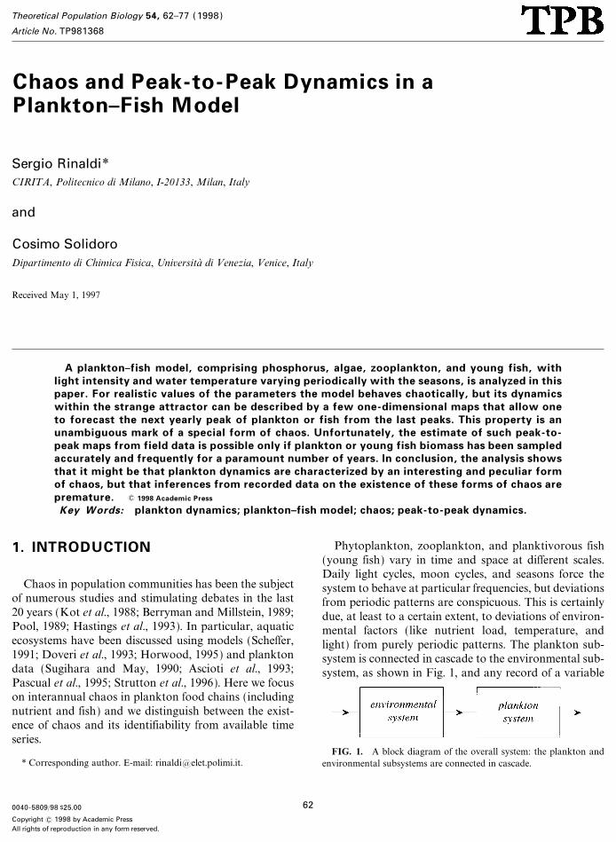
Phytoplankton, zooplankton, and planktivorous fish(young fish) vary in time and space at different scales.Daily light cycles, moon cycles, and seasons force thesystem to behave at particular frequencies, but deviationsfrom periodic patterns are conspicuous. This is certainlydue, at least to a certain extent, to deviations of environ-mental factors (like nutrient load, temperature, andlight) from purely periodic patterns. The plankton sub-system is connected in cascade to the environmental sub-system, as shown in Fig. 1, and any record of a variable

FIG. 1. A block diagram of the overall system: the plankton andenvironmental subsystems are connected in cascade.

Article No. TP981368

620040-5809�98 K25.00

Copyright ] 1998 by Academic PressAll rights of reproduction in any form reserved.

* Corresponding author. E-mail: rinaldi�elet.polimi.it.

File: DISTL2 136802 . By:CV . Date:06:07:98 . Time:07:56 LOP8M. V8.B. Page 01:01Codes: 6084 Signs: 5665 . Length: 54 pic 0 pts, 227 mm

of the plankton system contains also information on thedynamics of the environmental system. If we imagine thatthe two dynamical systems of Fig. 1 are described, respec-tively, by ne and np differential equations, the overallsystem will have (ne+np) Lyapunov exponents whichare a natural extension of the eigenvalues associated toan equilibrium (Guckenheimer and Holmes, 1983). Butthe fact that the two subsystems are connected in cascadeimplies that ne of these Lyapunov exponents are exactlythose of the environmental subsystem, while the remain-ing np depend upon the plankton subsystem as well asupon its input (which depends upon the environmentalsubsystem). Thus, counterintuitively, part of the infor-mation contained in any record of plankton or young fishconcerns only the environmental subsystem, part the mixof the two subsystems, but none has to do only withthe plankton subsystem. This is why plankton time seriesmight be potentially relevant for complementing orconfirming results obtained by analyzing purely oceano-graphic data at suitable scales (Ascioti et al., 1993;Pascual et al., 1995).

An interesting technical question is then the following:can the plankton system be chaotic if the environmentalsubsystem is cyclic? In other words, can the planktonsystem ``generate'' chaos? In practice, we know that theenvironmental system can be cyclic only in controlledlaboratory experiments, while in nature a more complexcomponent will be present. Thus, a rigorous answer toour question can be given only through modellingexercises or through suitably designed experiments.A positive answer to the above question implies that oneshould expect that the dominant Lyapunov exponent ofthe entire system of Fig. 1 could be greater than the domi-nant Lyapunov exponent of the environmental sub-system in regions with environmental factors varyingalmost periodically. In such a case, species interactionsand growth would be the real causes of the irregularitiesof observed plankton time patterns.

A great number of theoretical studies indicate that,indeed, plankton systems are, in principle, capable togenerate their own chaos. Prey-predator models (e.g.,phytoplankton�zooplankton communities) in seasonallyvarying environments have been proved to be chaotic forparticular parameter values (Inoue and Kamifukumoto,1984; Toro and Aracil, 1988; Schaffer, 1988; Kuztnesovet al., 1992; Rinaldi and Muratori, 1993; Rinaldi et al.,1993; Sabin and Summers, 1993) and the same holds forchemostat models where the prey feeds on a limitingnutrient (e.g., phosphorus) (Kot et al., 1992; Pavlou andKevrekidis, 1992; Gragnani and Rinaldi, 1995). On theother hand, tritrophic food chain models (e.g., phyto-plankton, zooplankton, young fish) have been shown to

behave chaotically in some niches of parameter spaceeven in a constant environment (Hogeweg and Hesper,1978; Scheffer, 1991; Hastings and Powell, 1991; Rai andSreenivasan, 1993; Klebanoff and Hastings, 1994;McCann and Yodzis, 1994; Wilder et al., 1994; McCannand Yodzis, 1995; Kuznetsov and Rinaldi, 1996).Moreover, competition for food (like that existingbetween different plankton communities) has also beenshown to be a potential source of deterministic chaos(Smale, 1976; Vance, 1978; Gilpin, 1979; Takeuchi andAdachi, 1983, Vandermeer, 1993). Finally, specificplankton models containing a mix of the above features(Scheffer, 1991; Doveri et al., 1993) have also been shownto behave chaotically for suitable parameter values.Thus, a natural question arises: why it has not yet beenpossible to verify unambiguously through time seriesanalysis that plankton is chaotic? One possible answer tothis question is that chaos does not exist (or is very rare)in natural ecosystems. This is not conflicting with theabove-mentioned results, because many of the modelsused to show that chaos is possible, also have enormousregions in parameter space which give stationary orcyclic solutions. Another possible answer is that currentdata are in any case too poor to identify chaos in aquaticecosystems. This is what we show in this paper, limitingthe analysis to interannual variability of algae, zoo-plankton, and fish. Similar results have been obtained ina study on gadoid populations (Horwood, 1995).

The paper is organized as follows. In the next sectionwe recall the notion of Poincare� section and map and weintroduce the notion of peak-to-peak dynamics (PPD).We also show that, if the strange attractor of a dynam-ical system is approximately one-dimensional on thePoincare� section, the peak of any relevant variable can beforecasted from the previous peak with one 1D map(simple PPD) or with K>1 1D maps (complex PPD).Then, in the following section we analyze a nutrient�algae�zooplankton�fish model (Doveri et al., 1993)assuming that the environment is purely periodic and weshow that a complex (K=3) PPD exists in such aplankton system. This PPD is a mark of the chaoticity ofthe aquatic ecosystem. Finally, we show with a series ofsystematic numerical experiments that the identificationof the PPD is practically impossible because it requires tosample plankton or fish biomass quite frequently withhigh accuracy for a paramount number of years. We alsoshow that random deviations of the environmentalvariables from their reference periodic patterns destroythe PPD itself, thus making the detection of chaos evenmore problematic. Merits and limitations of our studyare discussed at the end of the paper, together with somesuggestions for further research.

63Chaos and Peak-to-Peak Dynamics


PEAK-TO-PEAK DYNAMICS

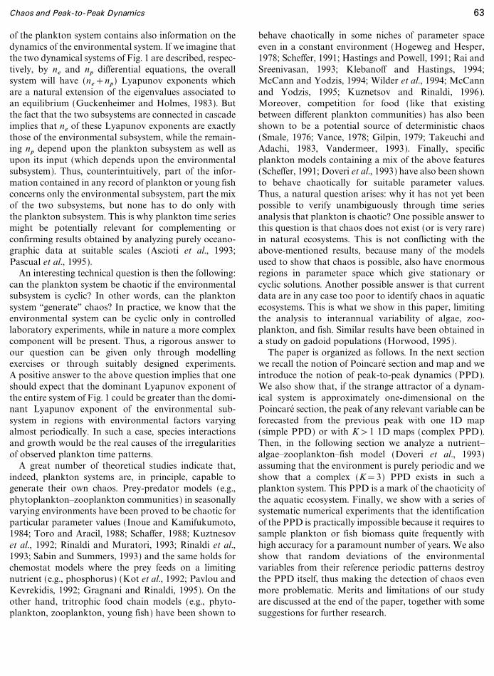
Let us consider a continuous-time autonomous systemx* =h(x), where x=(x1 , x2 , ..., xn) with n�3. Noticethat a periodically forced (n&1)-dimensional system canalways be given this form, by adding ``time'' as an extra-state variable, i.e., x* =1 (mod T ) where T is the period ofthe forcing function. Let us assume that such a systembehaves chaotically. Thus, its dynamics can be studied ona Poincare� section P, which is an (n&1)-dimensionalmanifold transversal to the strange attractor (Gucken-heimer and Holmes, 1983). Given a point z # P, the pointof first return z$ is uniquely identified by the Poincare�(first return) map z$=P(z) (see Fig. 2).

If the (fractal) dimension of the attractor is close to 2,i.e., if the attractor is approximately a surface, its inter-section A with P is approximately a line which can becoordinated with a single variable s, varying from 0 to 1.Thus, the dynamics ``within the attractor,'' namelyz$=P(z), z # A, can be approximately described by aone-dimensional (1D) map on the unit interval:

s$= f (s), 0�s�1, 0�s$�1. (1)

The existence of such 1D maps has been ascertained invarious fields of science, by analyzing models (e.g.,Arneodo et al., 1993; Freire et al., 1993) and data (e.g.,Guevara et al., 1981; Simoy et al., 1982; Roux, 1983;Roux et al., 1983; Argoul et al., 1993). In the second case

FIG. 2. A two-dimensional Poincare� section P of a three-dimen-sional continuous-time dynamical system x* =h(x), the intersection ofthe strange attractor with the Poincare� section (fractal set A) and theorbit going from point z # P to the first return point z$ # P. The dif-ferential equations x* =h(x) define a two-dimensional Poincare� map(first return map) z$=P(z).

the attractor must first be reconstructed from a timeseries using Packard's technique based on time-delaycoordinates (Packard et al., 1980; Ellner and Turchin,1995) and then intersected with a suitable Poincare� sec-tion. In population dynamics, 1D maps s$= f (s) havebeen discovered by analyzing models of periodicallyforced predator�prey communities (Schaffer, 1988; Kotet al., 1992) of tri-trophic food chains (Toro and Aracil,1988; Hastings and Powell, 1991) and of coupledprey�predators communities (Vandermeer, 1993) and byreconstructing strange attractors from time series ofchildhood epidemics in large towns (e.g., Schaffer andKot, 1985; Kot et al., 1988; Olsen et al., 1988).

The interest for 1D maps s$= f (s) is more conceptualthan operational. A relevant exception is the case ofpeak-to-peak maps which are defined on a particularPoincare� section, namely that on which one of the statevariables, say xj , is maximum. Since x* j=hj (x1 , ..., xn),this Poincare� section is identified by hj (x1 , ..., xn)=0.From now on the variable xj will be indicated by y andthe Poincare� section by Py , while the successive maximaof the variable y(t) and their times of occurrence will beindicated by yi and ti , i=1, 2, ... . In the case of peri-odically forced systems one must take into account thattime is measured (mod T). Thus, for example, in theapplication considered in this paper concerning interan-nual chaos of young planktivorous fish, T is equal to 365(days), yi is the maximum young fish biomass in year i,and ti is the day of the i th year at which fish biomass ismaximum.

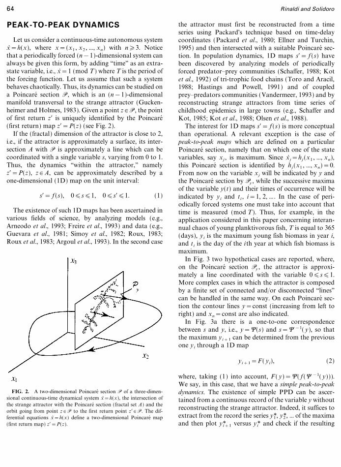
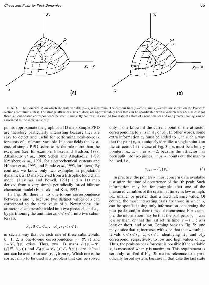
In Fig. 3 two hypothetical cases are reported, where,on the Poincare� section Py , the attractor is approxi-mately a line coordinated with the variable 0�s�1.More complex cases in which the attractor is composedby a finite set of connected and�or disconnected ``lines''can be handled in the same way. On each Poincare� sec-tion the contour lines y=const (increasing from left toright) and xn=const are also indicated.

In Fig. 3a there is a one-to-one correspondencebetween s and y, i.e., y=9(s) and s=9 &1( y), so thatthe maximum yi+1 can be determined from the previousone yi through a 1D map

yi+1=F ( yi), (2)

where, taking (1) into account, F ( y)=9( f (9 &1( y))).We say, in this case, that we have a simple peak-to-peakdynamics. The existence of simple PPD can be ascer-tained from a continuous record of the variable y withoutreconstructing the strange attractor. Indeed, it suffices toextract from the record the series y*1 , y*2 , ... of the maximaand then plot y*i+1 versus yi* and check if the resulting

64 Rinaldi and Solidoro


FIG. 3. The Poincare� Py on which the state variable y=xj is maximum. The contour lines y=const and xn=const are shown on the Poincare�section (continuous lines). The strange attractors (sets of dots) are approximately lines that can be coordinated with a variable 0�s�1. In case (a)there is a one-to-one correspondence between s and y. By contrast, in case (b) two distinct values of s (one smaller and one greater than s1) can beassociated to the same value of y.

points approximate the graph of a 1D map. Simple PPDare therefore particularly interesting because they areeasy to detect and useful for performing peak-to-peakforecasts of a relevant variable. In some fields the exist-ence of simple PPD seems to be the rule more than theexception (see, for example, Basset and Hudson, 1988;Albahadily et al., 1989; Schell and Albahadily, 1989;Kreisberg et al., 1991, for electrochemical systems andHu� bner et al., 1993, and Pando et al., 1993, for lasers). Bycontrast, we know only two examples in populationdynamics: a 1D map derived from a tritrophic food chainmodel (Hastings and Powell, 1991) and a 1D mapderived from a very simple periodically forced bilinearchemostat model (Funasaki and Kot, 1993).

In Fig. 3b there is no one-to-one correspondencebetween s and y, because two distinct values of s cancorrespond to the same value of y. Nevertheless, theattractor A can be subdivided into two pieces A1 and A2 ,by partitioning the unit interval 0�s�1 into two subin-tervals,

A1 : 0�s�s1 , A2 : s1<s�1,

in such a way that on each one of these subintervals,k=1, 2, a one-to-one correspondence y=9k(s) ands=9 &1

k ( y) exists. Thus, two 1D maps F1( y)=91

( f (9 &11 ( y))) and F2( y)=92 ( f (9 &1

2 ( y))) are definedand can be used to forecast yi+1 from yi . Which one is thecorrect map to be used is a problem that can be solved

only if one knows if the current point of the attractorcorresponding to yi is in A1 or A2 . In other words, someextra information :1 must be added to yi in such a waythat the pair ( yi , :i) uniquely identifies a single point s onthe attractor. In the case of Fig. 3b, :i must be a binarypointer, i.e., :i=1 or :i=2, because the attractor hasbeen split into two pieces. Thus, :i points out the map tobe used, i.e.,

yi+1=F:i( yi). (3)

In practice, the pointer :i must concern data availablejust after the time of occurrence of the i th peak. Suchinformation may be, for example, that one of themeasured variables of the system at time ti is low or high,i.e., smaller or greater than a fixed reference value. Ofcourse, the most interesting cases are those in which :i

can be specified using only information concerning thepast peaks and�or their times of occurrence. For exam-ple, the information may be that the past peak yi&1 waslow or high, or that the last return time (ti&ti&1) waslong or short, and so on. Coming back to Fig. 3b, onemay notice that xn increases with s, so that the two subin-tervals 0�s�s1 , s1<s�1 identifying A1 and A2 ,correspond, respectively, to low and high values of xn .Thus, the peak-to-peak forecast is possible if the variablexn is measured when y is maximum. This requirement iscertainly satisfied if Fig. 3b makes reference to a peri-odically forced system, because in that case the last state



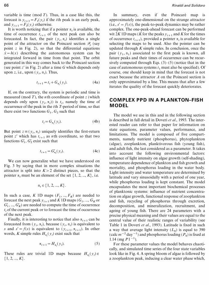
variable is time (mod T). Thus, in a case like this, theforecast is yi+1=F1( yi) if the i th peak is an early peak,and yi+1=F2( y i) otherwise.

It is worth noticing that if a pointer :i is available, thetime of occurrence t i+1 of the next peak can also beforecasted. In fact, the pair ( yi , :i) identifies a singlepoint of the attractor on the Poincare� section Py (saypoint z in Fig. 2), so that the differential equationsx* =h(x) describing the autonomous system can beintegrated forward in time from that point. The orbitgenerated in this way comes back to the Poincare� section(see point z$ in Fig. 2) after a time G which depends onlyupon z, i.e., upon ( yi , :i). Thus,

ti+1=ti+G:i( yi). (4a)

If, on the contrary, the system is periodic and time ismeasured (mod T), the n th coordinate of point z (whichdepends only upon ( yi , :i)) is ti , namely the time ofoccurrence of the peak in the ith T-period of time, so thatthere exist two functions G1 , G2 such that

ti=G:i( yi). (4b)

But point z#( yi , :i) uniquely identifies the first-returnpoint z$ which has ti+1 as n th coordinate, so that twofunctions G$1 , G$2 exist such that

ti+1=G$:i( y i). (4c)

We can now generalize what we have understood onFig. 3 by saying that in more complex situations theattractor is split into K>2 distinct pieces, so that thepointer :i must be an element of the set [1, 2, ..., K], i.e.

:i # [1, 2, ..., K].

In such a case, K 1D maps (F1 , ..., FK) are needed toforecast the next peak yi+1 and K 1D maps (G1 , ..., GK orG$1 , ..., G$K) are needed to compute the time of occurrenceti of the current peak or to forecast the time of occurrenceof the next peak.

Finally, it is interesting to notice that also :i+1 can beforecasted from ( yi , :i), because ( yi , :i) is equivalent tos and s$= f (s) is equivalent to ( yi+1 , :i+1). In otherwords, K simple rules H:i

( y i) exist such that

:i+1=H:i( y i). (5)

These rules are trivial 1D maps because H:i( yi) #

[1, 2, ..., K].

In summary, even if the Poincare� map isapproximately one-dimensional on the strange attractor(i.e., s$= f (s)), the peak-to-peak dynamics may be rathercomplex. The one-peak-ahead forecast can be performedwit 2K 1D maps (K for the peaks yi+1 and K for the timesof occurrence ti+1), provided a pointer :i is available forselecting the maps to be used. Also the pointer can beupdated through K simple rules. In conclusion, once thepair ( y1 , :1) associated to the first peak is known, allfuture peaks and their times of occurrence can be recur-sively computed through Eqs. (3)�(5) (notice that in thecase of autonomous systems t1 must also be specified). Ofcourse, one should keep in mind that the forecast is notexact because the attractor A on the Poincare� section isonly approximated by a line. This means that after a fewiterates the quality of the forecast quickly deteriorates.

COMPLEX PPD IN A PLANKTON�FISHMODEL

The model we use in this and in the following sectionis described in full detail in Doveri et al., 1993. The inter-ested reader can refer to that paper for information onstate equations, parameter values, performance, andlimitations. The model is composed of five compart-ments, namely nutrient (phosphorus), phytoplankton(algae), zooplankton, planktivorous fish (young fish),and adult fish, the last considered as a parameter. It takesinto account the following environmental factors:influence of light intensity on algae growth (self-shading),temperature dependence of plankton and fish growth andmortality, and phosphorus loading in the water body.Light intensity and water temperature are determined bylatitude and vary sinusoidally with a period of one year,while phosphorus loading is kept constant. The modelencapsulates the most important biochemical processesof planktonic systems: influence of nutrient concentra-tion on algae growth, functional response of zooplanktonand fish, recycling of phosphorus through excretion,decomposition, and mineralization, recruitment, andageing of young fish. There are 24 parameters with aprecise physical meaning and their values are equal to thecentral value of their realistic ranges of variability (seeTable 1 in Doveri et al., 1993). Latitude is fixed in sucha way that average light intensity (L0) is equal to 390(calc m&2 day&1) and phosphorus loading (P0) is fixed at1.14 (mg P1&1).

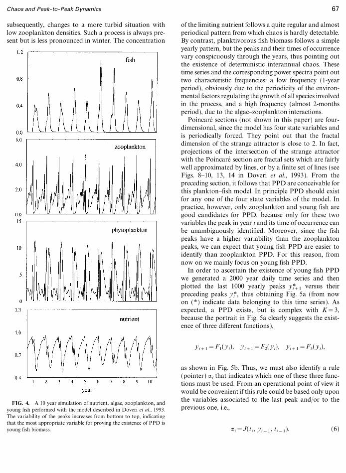
For these parameter values the model behaves chaoti-cally, and simulated time series of the four state variableslook like in Fig. 4. A spring bloom of algae is followed bya zooplankton peak, inducing a clear water phase which,



subsequently, changes to a more turbid situation withlow zooplankton densities. Such a process is always pre-sent but is less pronounced in winter. The concentration

FIG. 4. A 10 year simulation of nutrient, algae, zooplankton, andyoung fish performed with the model described in Doveri et al., 1993.The variability of the peaks increases from bottom to top, indicatingthat the most appropriate variable for proving the existence of PPD isyoung fish biomass.

of the limiting nutrient follows a quite regular and almostperiodical pattern from which chaos is hardly detectable.By contrast, planktivorous fish biomass follows a simpleyearly pattern, but the peaks and their times of occurrencevary conspicuously through the years, thus pointing outthe existence of deterministic interannual chaos. Thesetime series and the corresponding power spectra point outtwo characteristic frequencies: a low frequency (1-yearperiod), obviously due to the periodicity of the environ-mental factors regulating the growth of all species involvedin the process, and a high frequency (almost 2-monthsperiod), due to the algae�zooplankton interactions.

Poincare� sections (not shown in this paper) are four-dimensional, since the model has four state variables andis periodically forced. They point out that the fractaldimension of the strange attractor is close to 2. In fact,projections of the intersection of the strange attractorwith the Poincare� section are fractal sets which are fairlywell approximated by lines, or by a finite set of lines (seeFigs. 8�10, 13, 14 in Doveri et al., 1993). From thepreceding section, it follows that PPD are conceivable forthis plankton�fish model. In principle PPD should existfor any one of the four state variables of the model. Inpractice, however, only zooplankton and young fish aregood candidates for PPD, because only for these twovariables the peak in year i and its time of occurrence canbe unambiguously identified. Moreover, since the fishpeaks have a higher variability than the zooplanktonpeaks, we can expect that young fish PPD are easier toidentify than zooplankton PPD. For this reason, fromnow on we mainly focus on young fish PPD.

In order to ascertain the existence of young fish PPDwe generated a 2000 year daily time series and thenplotted the last 1000 yearly peaks y*i+1 versus theirpreceding peaks yi*, thus obtaining Fig. 5a (from nowon (*) indicate data belonging to this time series). Asexpected, a PPD exists, but is complex with K=3,because the portrait in Fig. 5a clearly suggests the exist-ence of three different functions),

yi+1=F1( yi), yi+1=F2( yi), yi+1=F3( yi),

as shown in Fig. 5b. Thus, we must also identify a rule(pointer) :i that indicates which one of these three func-tions must be used. From an operational point of view itwould be convenient if this rule could be based only uponthe variables associated to the last peak and�or to theprevious one, i.e.,

:i=J(ti , yi&1 , ti&1). (6)



FIG. 5. Using the model described in Doveri et al., 1993, a daily time series of young fish biomass over 2000 years has been produced. Dis-regarding the first 1000 years and extracting the highest value yi* of each remaining year, a series of 1000 peaks has been obtained. In (a) each peaky*i+1 , is plotted vs the previous peak yi*. In (b) the same points have been indicated with three different marks identifying the functions F1 , F2 , F3

needed to forecast the next peak with Eq. (3). The points ( yi*, y*i+1) with the same mark identify the sets Ik=[i | y*i+1$Fk( yi*)], k=1, 2, 3.

For discovering if a rule of this sort exists, we partitionedthe set of the years composing our time series in threesubsets I1 , I2 , and I3 as

Ik=[i | y*i+1$Fk( yi*)], k=1, 2, 3.

In other words, year i belongs to the set Ik if the functionFk is needed to forecast y*i+1 from yi*. Then, we first con-jectured that rule (6) was based only upon the time ofoccurrence of the last peak, i.e.,

:i=J(ti). (7)

To validate or reject this conjecture we determined thethree sets,

T k*=[ti* | i # Ik], k=1, 2, 3,

and checked if the time segment 1�t�365 could be par-titioned into three disjoint subintervals Tk with T*k /Tk ,k=1, 2, 3. Obviously, if this would be possible, thefollowing would be a well-defined pointer of the form (7)

:i=k � ti # Tk .

Since in our case the three disjoint intervals T1 , T2 , T3

did not exist the conjecture was rejected.At this point we repeated the analysis by making

reference to a new (second) conjecture, namely that rule(6) was based only upon the previous peak, i.e.,

:i=J( yi&1).

Thus, the following three sets,

Y*k=[ y*i&1 | i # Ik], k=1, 2, 3,

were determined. Since these sets do not belong to threeseparated intervals, this conjecture was rejected also.The same happened for the third conjecture, namely:i=J(ti&1).

We were therefore forced to look for rules of the form(6) with two independent variables. Our next choice wasto conjecture the existence of a pointer based on the timesof occurrence of the last two peaks, i.e.,

:i=J(ti , ti&1).

Thus we constructed the three sets,

[(ti*, t*i&1) | i # Ik], k=1, 2, 3,



FIG. 6. The sets [(t*i&1 , ti*) | i # Ik)], k=1, 2, 3, produced from the time series ( yi*, ti*), i=1, ..., 1000, taking into account Fig. 5b. The three setscan be seperated by partitioning the space in three subregions.

FIG. 7. The 1000 points ( yi*, ti*) of the time series plotted in (a) indicate the three functions G1 , G2 , G3 used in Eq. (4b). Similarly, the points( yi*, t*i+1) in (b) indicate the functions G$1 , G$2 , G$3 needed to forecast the time of occurrence of the next peak through Eq. (4c).



and verified, as shown in Fig. 6, that they can beseparated by partitioning the space (ti , ti&1) in threeregions. This validates the conjecture and the pointer :i

can be specified with only two parameters (critical days)in the following very simple way:

1 � t i�255, ti&1�215;

:i={2 � ti�255, t i&1>215;

3 � t i>255.

The result states that if the last peak yi is a late peak (i.e.,a peak with ti>255), the next peak yi+1 is given byyi+1=F3( yi), where the function F3 is reported inFig. 5b. By contrast, if the last peak is not a late peak (i.e.,ti�255), one cannot forecast the next peak yi+1 withoutknowing also the time of occurrence ti&1 of the previouspeak.

It is worth noticing that also the time of occurrence ti

(ti+1) of the current (next) peak can be computed(forecasted) from yi and :i , (see Eq. (4b) ((4c))), providedthat the three functions G1 , G2 , G3 (G$1 , G$2 , G$3) areestimated by interpolating the three sets [t i*, yi*) | i # Ik]([(t*i+1 , yi*) | i # Ik]), k=1, 2, 3, as indicated in Fig. 7.

Finally one may notice that :i+1 can be easilycomputed from the pair ( yi , :i), as stated in the previoussection, since

:i+1=J(t i+1 , t i)=J(G$:i( yi), G:i

( yi)). (9)

This definitely shows that, given the pair ( yi , :i) charac-terizing a first peak, all subsequent peaks and their timesof occurrence can virtually be computed through a recur-sive scheme.

DIAGNOSING INTERANNUAL CHAOSIN PLANKTON�FISH COMMUNITIES

We now focus on the identifiability of the plankton�fish interannual chaos from time series. We deal with thisproblem in three independent ways that give roughly thesame answer. The first is a simple analogy betweenplanktonic and cardiac systems for which chaos charac-teristics are identifiable through ECG. The second isthe estimation of classical invariants, like Lyapunovexponents and noninteger dimension. The third is theidentifiability of the PPD we have pointed out in thepreceding section.

A Simple Analogyy Chaos in ECG

The plankton�fish interannual chaos discussed inDoveri et al. (1993) is due to the interference betweenperiodic exogenous forces (seasons) with the natural2-months oscillatory behavior of the system, due toalgae�zooplankton interactions. Chaos in periodicallyforced oscillators is perhaps the most common formof irregular behavior of dynamical systems. It hasbeen studied theoretically (e.g., Guckenheimer andHolmes, 1983; Gambaudo, 1985; Namachchivaya andAriaratnam, 1987) and many applications. The cardiacsystem is another example of periodically forced system,since the heart, beating once per second, is perturbed bythe breathing cycle, which has approximately a period of6 s. Thus, planktonic systems and cardiac systems areperiodically forced oscillators characterized by the sameratio (1 :6) between exogenous and endogenous frequen-cies. On the basis of this analogy, we might be inclined toimagine that the amount of data necessary to detectdeterministic chaos from ECG is a good estimate of theamount of data required to recognize chaos in a planktontime series. Six hours ECG have been shown to be suf-ficient for reconstructing strange attractors of the cardiacsystem (Schmidt and Morfill, 1994; Guzzetti et al., 1996).Since 6 h correspond to 3600 breathing cycles, we canimagine that the same number of forcing period (i.e.,years) are needed for the planktonic system. The result ofthis na@� ve analogy is astonishing; plankton�fish timeseries should be a few thousand years long in order toreveal that they contain deterministic chaos.

Estimation of Invariants

Estimation of invariants of strange attractors fromtime series has been the subject of numerous studies (e.g.,Ruelle, 1987; Sugihara and May, 1990; Kennel andIsabelle, 1992; Mitschke and Da� mming, 1993).

Moon (1987) has summarized his experiences bystating that at least 4000 points on a Poincare� sectionmust be available before concluding that a system ischaotic. This means that planktonic systems should besampled for 4000 years, a figure that agrees with the con-clusion drawn from the analogy with the cardiac system.Other authors (Eckmann et al., 1986; Farmer andSidorowich, 1987; Abarbanel et al., 1990; Casdagli, 1991;Wolf and Bessoir, 1991; Ellner et al., 1991) state thattypical values of data length for identifying the dynamicsof a system is order 104. In particular, for the estimate ofLyapunov exponents it has been argued that 103�104

forcing periods are needed (Denton and Diamond, 1991)while another estimate is 30d, where d is the dimension



(in the plankton�fish model considered in this paper d isclose to 2 so that this estimate is order 103). For esti-mating the dimension of the attractor larger data recordsare usually needed (Wolf and Bessoir, 1991). Typicalexamples use more than 104 data points, but a recenttechnique, based on NARMAX models, seems to requireonly 103 data points (Aguirre and Billings, 1995).

In any case, all above-mentioned contributionssuggest that at least 1000 years of plankton�fish datashould be available for proving that the planktonicsystem is characterized by interannual chaos.

PPD Identifiability

We now look at the identifiability of the plankton�fishinterannual chaos using the notion of PPD introducedabove. The three peak-to-peak maps F1 , F2 , F3 defined inthe preceding section are the mark of a strange attractor.It is therefore interesting to know how many data arenecessary for identifying these maps. For answering thisquestion, first we have simulated our plankton�fishsystem for 1000 years. Then we have sampled young fishbiomass every day, thus creating a reference time series.From this reference time series we have extracted threedaily time series of 500, 200, and 50 years length denoted,respectively, a1 , a2 , and a3 . Sampling the reference timeseries every 7, 14, 28 days we have generated three othersurrogate series, called b1 , b2 , b3 . Finally, we have alsoadded to each element y of the reference time series ameasurement error =y, where = was a randomly gener-ated variable with uniform distribution in the interval[&0.1, 0.1]. We have then repeated this operation withthe intervals [&0.3, 0.3] and [&0.5, 0.5], thus gener-ating three surrogate time series indicated by c1 , c2 , c3

corresponding, respectively, to 10, 30, and 50 0 maxi-mum errors in measuring fish biomass.

Then, for each one of the above time series, we haveconstructed a peak time series ( yi*, t i*) and plotted thepairs ( yi*, y*i+1) in a two-dimensional space. The por-traits obtained with the time series ai , bi , and ci , areshown in the first, second, and third rows of Fig. 8,respectively. Each portrait of Fig. 8 should be comparedwith Fig. 5a which was used in the preceding section toidentify the three 1D maps F1 , F2 , F3 shown in Fig. 5b.

The first row of Fig. 8 clearly indicates that, even in theideal case of one sample per day and no measurementerrors, 50 years of data would not be enough for identi-fying the peak-to-peak maps F1 , F2 , F3 . The second rowshows that sampling fish biomass once a week, instead ofonce a day, does not seriously affect the identifiability ofthe three peak-to-peak maps, while sampling once every

four weeks introduces detectable errors but does notdestroy the possibility of recognizing the presence ofchaos. The low impact of the sampling period can beexplained by noticing that the yearly maxima yi* used inthe second row of Fig. 8 are not the highest yearlysamples of biomass but an estimate of the true maximaobtained through a suitable parabolic interpolation ofthe samples. A comparison with the portraits producedby plotting the highest yearly samples (not shown in thefigure) indicates that the parabolic interpolation drama-tically attenuates the impact of the sampling period.Finally, the last row shows that the level of the measure-ment noise seriously affects the identifiability of the peak-to-peak maps, up to the point that the existence of threemaps can hardly be suspected with a 300 measurementerror.

The reference time series used to produce Fig. 8 wasgenerated by simulating the model with constant nutrientloading and periodically varying light intensity andwater temperature. As already remarked, if the environ-mental variables would deviate from their reference pat-terns, the PPD would change or eventually be destroyedif the new strange attractor would not have low dimen-sions. To detect the influence of the environmental noisewe have therefore created six new surrogate time seriesby randomly perturbing nutrient loading and light inten-sity. More precisely, we have simulated the system for1000 years, changing the nutrient loading every four daysby adding to its reference value P0 a random variable =P0

with = uniformly distributed in three different intervals[&0.02, 0.02], [&0.05, 0.05], [&0.1, 0.1]. Then, wehave sampled young fish biomass once a day, thusgenerating three time series denoted by d1 , d2 , and d3 . Inanother simulation we have varied light intensity in thesame way and produced three time series e1 , e2 , e3

corresponding to increasing levels of weather variability(2, 5, and 100). From this time series we have extractedthe highest fish biomass yearly samples yi* and plottedthe pairs ( yi*, y*i+1). The results are shown in Fig. 9 andindicate that PPD are practically insensitive to nutrientloading but quite sensitive to light intensity. The first factis not a surprise if one recognizes that phosphorus is notlimiting algal growth, since phosphorus concentration(see Fig. 4) is plainly above the half saturation constantof nutrient uptake, which falls in the range [0.01, 0.03],as indicated in Table 1 of Doveri et al. (1993).

Up to now, we have analyzed the impact that variousfactors have on the identifiability of the three peak-to-peak maps F1 , F2 , F3 by activating only one factor at atime. When all factors are active the results are even morediscouraging. Figure 10 shows, for example, what couldbe obtained by sampling fish biomass for 1000, 200, and



FIG. 8. Each portrait is the plot of the pairs ( yi*, y*i+1) of a different time series (see text). Comparing with Fig. 5a one can detect the influencesthat different factors have on the identifiability of the three peak-to-peak maps F1 , F2 , F3 . The first row shows the effect of the length of the time series.The second row shows that the sampling period has a low impact on the identifiability of the maps (see text for a justification). The third row showsthat measurement errors pulverize the maps.

40 years every 14 days with a 300 maximum measure-ment error and in the presence of 50 maximumvariability of nutrient loading and light intensity. Theexistence of the three maps is not even revealed by 1000years of data while the existence of PPD is hardly detec-table with 200 years of data. This analysis is therefore inline with the indications coming from the analogy withthe cardiac system and with the experiences reported

by different authors on the difficulties in estimatinginvariants of strange attractors.

We conclude this section by showing that planktontime series are even less promising than young fishtime series, if the aim is to detect the existence of deter-ministic chaos. Figure 11 reports in the first row threeportraits referring to zooplankton data. The first one(daily samples, no measurement errors, no environmental



FIG. 9. The effects of environmental variability on the identifiability of the maps F1 , F2 , F3 shown in Fig. 5b. The first row shows that thevariability of the nutrient loading has no impact (see text for a justification). The second row shows that light variability pulverizes the three maps.

FIG. 10. Three portraits ( yi*, y*i+1) obtained from three realistic time series (14 days sampling period, 300 measurement error, and 50 environ-mental variability). These portraits should be compared with Fig. 5a where the sampling period is one day and there is no measurement and environ-mental noise. The three peak-to-peak maps are pulverized and cannot be identified even with 1000 years of data. Nevertheless, their existence canbe reasonably conjectured even with 200 years of data.



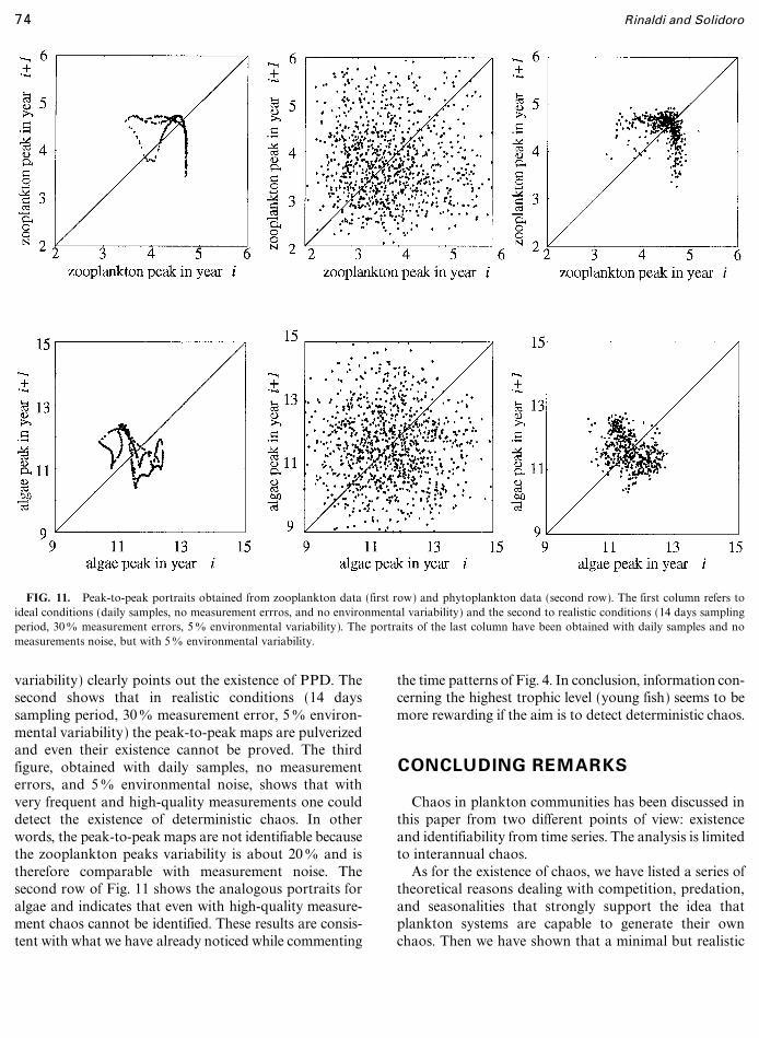
FIG. 11. Peak-to-peak portraits obtained from zooplankton data (first row) and phytoplankton data (second row). The first column refers toideal conditions (daily samples, no measurement errros, and no environmental variability) and the second to realistic conditions (14 days samplingperiod, 300 measurement errors, 50 environmental variability). The portraits of the last column have been obtained with daily samples and nomeasurements noise, but with 50 environmental variability.

variability) clearly points out the existence of PPD. Thesecond shows that in realistic conditions (14 dayssampling period, 300 measurement error, 50 environ-mental variability) the peak-to-peak maps are pulverizedand even their existence cannot be proved. The thirdfigure, obtained with daily samples, no measurementerrors, and 50 environmental noise, shows that withvery frequent and high-quality measurements one coulddetect the existence of deterministic chaos. In otherwords, the peak-to-peak maps are not identifiable becausethe zooplankton peaks variability is about 200 and istherefore comparable with measurement noise. Thesecond row of Fig. 11 shows the analogous portraits foralgae and indicates that even with high-quality measure-ment chaos cannot be identified. These results are consis-tent with what we have already noticed while commenting

the time patterns of Fig. 4. In conclusion, information con-cerning the highest trophic level (young fish) seems to bemore rewarding if the aim is to detect deterministic chaos.

CONCLUDING REMARKS

Chaos in plankton communities has been discussed inthis paper from two different points of view: existenceand identifiability from time series. The analysis is limitedto interannual chaos.

As for the existence of chaos, we have listed a series oftheoretical reasons dealing with competition, predation,and seasonalities that strongly support the idea thatplankton systems are capable to generate their ownchaos. Then we have shown that a minimal but realistic



model has a specific form of interannual chaos that canbe described through three 1D peak-to-peak maps. Thismeans, for example, that the next year peak of young fishbiomass can be forecasted with one of these three mapsfrom the peak of the present year. The choice of the mapto be used is based on the times of occurrence of thepeaks of the current and last years.

The identifiability of deterministic chaos in plankton�fish time series has been discussed in three different ways.First, by making an analogy with another periodicallyforced system, namely the cardiac system. Second, bylooking at the experiences on reconstructing strangeattractors and estimating their invariants reported in theliterature during last decade. Finally, by performing aseries of experiments based on surrogate data and aimedat the identification of the peak-to-peak maps. The threeapproaches indicate that the time series should be verylong (i.e., at least a few hundred years long) in order tohave some chances to distinguish chaos from noise.Other results of our analysis are the following. The sam-ples can be performed every two weeks, provided a goodscheme for reconstructing the times of occurrence of thelast peak is available. Measurement error are quite criti-cal, in particular when dealing with algae concentrationand zooplankton biomass, because the variations of theyearly algae and zooplankton peaks fall in the range ofmeasurement noise. By contrast, high frequency environ-mental noise, in particular variability of nutrient loading,is not affecting the data at the point of inhibiting thepossibility of detecting the existence of deterministicchaos. In conclusion, the result of our study is thefollowing: interannual chaos in plankton�fish com-munities may exist, but even if it does it would not bepossible to detect it with the data available nowadays.

For enhancing the possibility of detecting chaos froma time series one could perhaps follow a more articulateapproach. Using data collected during periods far fromthe expected occurrence of the yearly peaks and even-tually complementing these data with special laboratoryand field experiments, one could calibrate the parametersof a plankton�fish model of the kind used in this paper.Then, the calibrated model could be used to ascertain theexistence of peak-to-peak maps. If the answer is positive,the form of the peak-to-peak maps produced by thecalibrated model could be used to define a paremetrizedfamily of peak-to-peak maps. Finally one could select,within this family, the map that fits the yearly peaks best.This procedure, makes a more complete use of the dataset (notice that in our analysis only the yearly peaks areused) and is aligned with the classical philosophy ofsystem identification: use field data to estimate param-eters of mathematical models and then use the models to

extrapolate system behavior. Nevertheless, one should berather cautious, since ideas of this sort have alreadyproved to be of dubious impact in population dynamics(Morris, 1990).

Finally, we like to stress that the approach we havefollowed in this paper to discover peak-to-peak dynamicsin a plankton�fish model can be applied to any con-tinuous-time model. This is certainly a valuable point inecology and population dynamics, where blooms, out-breaks, and demographic explosions are very often theepisodes that one would like to forecast.

ACKNOWLEDGMENTS

This study has been financially supported by the Italian Ministry ofScientific Research and Technology, under Contract MURST 400Teoria dei sistemi e del controllo. Part of the work has been carried outat the International Institute for Applied Systems Analysis (IIASA),Laxenburg, Austria.

REFERENCES

Abarbanel, H. D. I., Brown, R., and Kadtke, J. B. 1990. Prediction inchaotic nonlinear systems: methods for time series with broadbandFourier spectra, Phys. Rev. A 41, 1782�1807.

Albahadily, F. N., Ringland, J., and Schell, M. 1989. Mixed-modeoscillations in an electrochemical system. I. A Farey sequence whichdoes not occur on a torus, J. Chem. Phys. 90, 813�821.

Aguirre, L. A., and Billings, S. 1995. Retriving dynamical invariantsfrom chaotic data using NARMAX models, Int. J. Bif. Chaos 5,449�474.

Argoul, F., Huth, J., Merzeau, P., Arneodo, A., and Swinney, H. L.1993. Experimental evidence for homoclinic chaos in an electro-chemical growth process, Physica D 62, 170�185.

Arneodo, A., Argoul, F., Elezgaray, J., and Richetti, P. 1993.Homoclinic chaos in chemical systems, Physica D 62, 134�169.

Ascioti, F. A., Beltrami, E., Carroll, T. O., and Wirick, C. 1993. Is therechaos in plankton dynamics? J. Plankton Res. 15, 603�617.

Bassett, M. R., and Hudson, J. L. 1988. Shil'nikov chaos during copperelectrodissolution, J. Phys. Chem. 92, 6963�6966.

Berryman, A. A., and Millstein, J. A. 1989. Are ecological systemschaotic��and if not, why not? Trends Ecol. Evol. 4, 26�28.

Casdagli, M. 1991. Chaos and deterministic versus stocastic non-linearmodelling, J. R. Stat. Soc. B 54, 303�328.

Denton, T. A., and Diamond, G. A. 1991. Can the analytic techniquesof non linear dynamics distinguish periodic, random and chaoticsignals? Comput. Biol. Med. 21, 243�264.

Doveri, F., Scheffer, M., Rinaldi, S., Muratori, S., and Kuznetsov, Y. A.1993. Seasonality and chaos in a plankton-fish model, Theor. Pop.Biol. 43, 159�183.

Eckmann, J. P., Kamphorst, S. O., Ruelle, D., and Ciliberto, S. 1986.Liapunov exponents from time series, Phys. Rev. A 34, 4971�4979.

Ellner, S., Gallant, A. R., McCaffrey, D., and Nychka, D. 1991. Con-vergence rates and data requirements for Jacobian-based estimatesof Lyapunov exponents from data, Phys. Lett. 153, 357�363.



Ellner, S., and Turchin, P. 1995. Chaos in a noisy word: New methodsand evidence from time-series analysis, Am. Natur. 145, 343�375.

Farmer, J. D., and Sidorowich, J. J. 1987. Predicting chaotic time series,Phys. Rev. Lett. 59, 845�848.

Freire, E., Rodriguez-Luis, A. J., Gamero, E., and Ponce, E. 1993.A case study for homoclinic chaos in an autonomous electroniccircuit, Physica D 62, 230�253.

Funasaki, E., and Kot, M. 1993. Invasion and chaos in a periodicallypulsed mass-action chemostat, Theor. Popul. Biol. 44, 203�224.

Gambaudo, J. M. 1985. Perturbation of a Hopf bifurcation by an exter-nal time-periodic forcing, J. Differential Eqs. 57, 172�199.

Gilpin, M. E. 1979. Spiral chaos in a predator�prey model, Amer.Natur. 113, 306�308.

Gragnani, A., and Rinaldi, S. 1995. A universal bifurcation diagram forseasonally perturbed predator�prey models, Bull. Math. Biol. 57,701�712.

Guckenheimer, J., and Holmes, P. 1983. ``Nonlinear Oscillations,Dynamical Systems and Bifurcation of Vector Fields,'' Springer-Verlag, New York.

Guevara, M. R., Glass, L., and Shrier, A. 1981. Phase-locking, period-doubling bifurcations and irregular dynamics in periodicallystimulated cardiac cells, Science 214, 1350�1353.

Guzzetti, S., Signorini, M. G., Cogliati, C., Mezzetti, S., Porta, A.,Cerutti, S., and Malliani, A. 1996. Deterministic chaos indices inheart rate variability of normal subjects and heart transplantedpatients, Cardiovasc. Res. 31, 441�446.

Hastings, A., and Powell, T. 1991. Chaos in a three species food chain,Ecology 72, 896�903.

Hastings, A., Hom, C. L., Ellner, S., Turchin, P., and Godfray, H. C. J.1993. Chaos in ecology: is mother nature a strange attractor? Annu.Rev. Ecol. Syst. 24, 1�33.

Hogeweg, P., and Hesper, B. 1978. Interactive instruction on popula-tion interaction, Comp. Biol. Med. 8, 319�327.

Horwood, J. 1995. Plankton-generated chaos in the modelled dynamicsof haddock, Phil. Trans. R. Soc. Lond. B 350, 109�118.

Hu� bner, U., Weiss, C. O., Abraham, N. B., and Tang, D. 1993. Lorenz-like chaos in NH3-FIR lasers, in ``Time Series Prediction: Fore-casting the Future and Understanding the Past'' (A. S. Weighandand N. A. Gersenfeld, Eds.), Addison�Wesley, Reading, MA.

Inoue, M., and Kamifukumoto, H. 1984. Scenarios leading to chaos inforced Lotka�Volterra model, Progr. Theor. Phys. 71, 930�937.

Kennel, M. B., and Isabelle, S. 1992. Method to distinguish possiblechaos from colored noise and to determine embedding parameters,Phys. Rev. A 46, 3111�3118.

Klebanoff, A., and Hastings, A. 1994. Chaos in three-species foodchains, J. Math. Biol. 32, 427�451.

Kot, M., Sayler, G. S., and Schultz, T. W. 1992. Complex dynamics ina model microbial system, Bull. Math. Biol. 54, 619�648.

Kot, M., Schaffer, W. M., Truty, G. L., Graser, D. J., and Olsen, L. F.1988. Changing criteria for imposing order, Ecol. Modelling 43,75�110.

Kreisberg, N., McCormick, W. D., and Swinney, H. L. 1991.Experimental demonstration of subtleties in subharmonic intermit-tency, Physica D 50, 463�477.

Kuznetsov, Y. A., Muratori, S., and Rinaldi, S. 1992. Bifurcations andchaos in a periodic predator�prey model, Int. J. Bif. Chaos 2, 117�128.

Kuznetsov, Y. A., and Rinaldi, S. 1996. Remarks on food chaindynamics, Math. Biosci. 134, 1�33.

McCann, K., and Yodzis, P. 1994. Biological conditions for chaos in athree-species food chain, Ecology 75, 561�564.

McCann, K., and Yodzis, P. 1995. Bifurcation structure of three-speciesfood chain model, Theor. Pop. Biol. 48, 93�125.

Mitschke, F., and Da� mming, M. 1993. Chaos versus noise inexperimental data, Int. J. Bif. Chaos. 3, 693�702.

Moon, F. C. 1987. ``Chaotic Vibrations��An Introduction for AppliedScientists and Engineers,'' Wiley, New York.

Morris, W. M. 1990. Problems in detecting chaotic behavior in naturalpopulation by fitting simple discrete models, Ecology 71, 1849�1862.

Namachchivaya, S. N., and Ariaratnam, S. T. 1987. Periodically per-turbed Hopf bifurcation, SIAM J. Appl. Math. 47, 15�39.

Olsen, L. F., Truty, G. L., and Schaffer, W. M. 1988. Oscillatios andchaos in epidemics: A nonlinear dynamic study of six childhooddiseases in Copenhagen, Denmark, Theor. Popul. Biol. 33, 344�370.

Packard, N., Crutchfield, J., Farmer, J., and Shaw, R. 1980. Geometryfrom a time series, Phys. Rev. Lett. 45, 712�716.

Pando, C. L., Meucci, R., Ciofini, M., and Arecchi, F. T. 1993. CO2

laser with modulated losses: theoretical models and experiments inthe chaotic regime, Chaos 3, 279�283.

Pascual, M., Ascioti, F. A., and Caswell, H. 1995. Intermittency inthe plankton: A multifractal analysis of zooplankton biomassvariability, J. Plankton Res. 17, 1209�1232.

Pavlou, S., and Kevrekidis, I. G. 1992. Microbial predation in a peri-odically operated chemostat: a global study of the interactionbetween natural and externally imposed frequencies, Math. Biosci.108, 1�55.

Pool, R. 1989. Ecologists flirt with chaos, Science 243, 310�313.Rai, V., and Sreenivasan, R. 1993. Period-doubling bifurcation leading

to chaos in a model food chain, Ecol. Modelling 69, 63�77.Rinaldi, S., and Muratori, S. 1993. Conditioned chaos in seasonally per-

turbed predator�prey models, Ecol. Modelling 69, 79�97.Rinaldi, S., Muratori, S., and Kuznetsov, Y. A. 1993. Multiple attrac-

tors, catastrophes and chaos in seasonally perturbed predator�preycommunities, Bull. Math. Biol. 55, 15�35.

Roux, J. C. 1983. Experimental studies of bifurcations leading to chaosin the Belusof�Zhabotinsky reaction, Physica D 7, 57�68.

Roux, J. C., Simoy, R. H., and Swinney, H. L. 1983. Observation of astrange attractor, Physica D 8, 257�266.

Ruelle, D. 1987. Diagnosis of dynamical systems with fluctuatingparameters, Proc. R. Soc. Lond. A 413, 5�8.

Sabin, G. C. W., and Summers, D. 1993. Chaos in a periodically forcedpredator�prey ecosystem model, Math. Biosci. 113, 91�113.

Schaffer, W. M. 1988. Perceiving order in the chaos of nature, in``Evolution of Life Histories of Mammals'' (M. S. Boyce, Ed.),pp. 313�350, Yale Univ. Press, New Haven, CT.

Schaffer, W. M., and Kot, M. 1985. Nearly one-dimensional dynamicsin an epidemic, J. Theor. Biol. 112, 403�427.

Schaffer, W. M., and Kot, M. 1986. Chaos in ecological systems: Thegoals that Newcastle forgot, Trends Ecol. Evol. 1, 58�63.

Scheffer, M. 1991. Should we expect strange attractors behind planktondynamics and if so, should we bother? J. Plankton Res. 13,1291�1305.

Schell, M., and Albahadily, F. N. 1989. Mixed-mode oscillations in anelectrochemical system. II. A periodic-chaotic sequence, J. Chem.Phys. 90, 822�828.

Schmidt, G., and Morfill, G. 1994. Complexity diagnostics in cardiol-ogy: Fundamental considerations, PACE 17, 1174�1177.

Simoy, R. H., Wolf, A., and Swiney, H. L. 1982. One dimensionaldynamics in a multicomponent chemical reaction, Phys. Rev. Lett.49, 245�248.

Smale, S. 1976. On the differential equations of species in competition,J. Math. Biol. 3, 5�7.

Strutton, P. G., Mitchell, J. G., and Parslow, J. S. 1996. Non-linearanalysis of clorophyll a transects as a method of quantifying spatialstructure. J. Plankton Res. 18, 1717�1726.



Sugihara, G., and May, R. M. 1990. Nonlinear forecasting as a way ofdistinguishing chaos from measurement error in time series, Nature344, 734�741.

Takeuchi, Y., and Adachi, N. 1983. Existence and bifurcation of stableequilibrium in two prey one predator communities, Bull. Math. Biol.45, 877�900.

Toro, M., and Aracil, J. 1988. Qualitative analysis of system dynamicsecological models, Syst. Dyn. Rev. 4, 56�80.

Vance, R. R. 1978. Predation and resource partitioning in one

predator�two prey model communities, Amer. Natur. 112, 797�813.Vandermeer, J. 1993. Loose coupling of predator�prey cycles: entrain-

ment, chaos, and intermittency in the classic MacArthur con-sumer�resource equations, Amer. Natur. 141, 687�716.

Wilder, J. W., Voorhis, N., Colbert, J. J., and Sharov, A. 1994. A threevariable differential equation model for gipsy moth populationdynamics, Ecol. Modelling 72, 229�250.

Wolf, A., and Bessoir, T. 1991. Diagnosing chaos in the space circle,Physica D 50, 239�258.

� � � � � � � � � � � � � � � � � � � �


Chaos and Peak-to-Peak Dynamics in a Plankton–Fish Model

Documents

Transcript of Chaos and Peak-to-Peak Dynamics in a Plankton–Fish Model