Channel State Feedback in MIMO SystemsChannel State Feedback in MIMO Systems

Dragan Samardzija and Professor Narayan Mandayam

Wireless Information Network Laboratory (WINLAB), Rutgers, the

State University of New Jersey, 73 Brett Road, Piscataway NJ 08854, USA

Bell Laboratories, Lucent TechnologiesWireless Research Laboratory

791 Holmdel-Keyport Rd.Holmdel, NJ 07733 USA

Page:2

Multiple Antenna SolutionsMultiple Antenna Solutions• Rely on [Tse-03]

• Spatial multiplexing• Diversity

• MIMO• Capacity gains understood under idealized assumptions [Foschini-96]• Need to understand

• Performance for multiuser systems• Frequency selective and time varying channels

• Multiple antenna transmitter optimizations in multiuser systems• Coherent [Farrohi-98, Visotsky-Madhow-99, Shamai-Caire-03, Goldsmith-03]

•• Rely on availability of CSI at transmitterRely on availability of CSI at transmitter•• Very sensitive to CSI mismatchVery sensitive to CSI mismatch

• Opportunistic beamforming [Laroia-Viswanath-03]• Dynamic subsectorization/fixed beams [Pedersen-03, Alamuti-04]

High Spectral Efficiency

Page:3

Talk OutlineTalk Outline

• Downlink multiple antenna multiuser optimization schemes

• Effects of CSI delay on the sum data rate

• Channel state prediction based on the MMSE criterion

• How to efficiently transmit CSI?

• We propose ‘zero-delay’ unquantized and uncoded (UQ-UC) CSI feedback

Page:4

TX Optimization TX Optimization -- System ModelSystem Model

x(1)

x(2)

x(3)

MIMO

Channel

H

TX

Transform

S

y(1)

y(2)

y(3)

Mobile 1

Mobile 2

Mobile 3

Transmitter

Assumed to be known at the TX

Page:5

Constraints and SimplificationsConstraints and Simplifications• Received signal

y = H S x + n

• S – spatial pre-filter is simplified as

S = A P A is a linear transformationP is a diagonal matrix

• Constraint total average power where power does not have to be equal among users

trace(AP PHAH) =Pmax

P is diagonal and selected to maximize sum rate

Page:6

Linear Transformation: Three SolutionsLinear Transformation: Three Solutions1. Zero Forcing

A = HH (H HH)-1

• Zero the interference

2. Modified ZF

A = HH (H HH + (No/ Pav)I )-1

• Tame zeroing of the interference

3. TriangularizationA= HH R-1

• H = (QR)H -Orthogonal-triangular decomposition• H A = L – lower triangular matrix• Preparing for Dirty Paper Coding

Using uplink/downlink duality we proved equivalence to the MMSE receiver.

We proved the optimality for high SNR.

Page:7

M = M = 3, 3, NN = 3= 3, , RayleighRayleigh Fading, Average RateFading, Average Rate

DPC approaches the MIMO case

MZF vs. ZF similar behavior to MMSE vs. ZF receiver

Significant gains versus conventional user multiplexing

Page:8

ZF and MZF Scheme, M = ZF and MZF Scheme, M = 3, 3, NN = = 3, SNR = 10dB 3, SNR = 10dB Average Rate for Correlated Channels vs. CSI DelayAverage Rate for Correlated Channels vs. CSI Delay

• More spatially correlated – more immune to the CSI delay.

• Worse than if no TX optimization is applied.

Page:9

MMSE Channel State PredictionMMSE Channel State Prediction• Goal of the transmitter it predicts future channel state h(τ) based on the

CSI h(t)• Prediction is to be done using a linear predictor W• To be designed based on minimum mean square criterion

MMSE = E[| WH hu - h(τ) H|2]

where is hu uber vector hu=[h(0) … h(-(K-1)T)]T

• Let us denoteU = E[hu hu

H] V = E[hu h(τ)]

W = U-1 V

• Exploits spatial and temporal correlations of the channel in MISO system

Estimated based on previous h(t)

Page:10

Uber vector hu(-1)

MMSE Prediction ImplementationMMSE Prediction Implementation

• Assuming stationary system, the estimates are used

• Predicted CSI is

• Assumptions and limitations• For duration of estimation LTupdate stationary is assumed• Nyquist condition Tupdate < 1/(2fdoppler)

h(0)h(-1)h(-2)h(-3)h(-4)h(-5)h(-6) h(τ)

Uber vector hu(0)

Uber vector hu(-2)Previous CSITo be predicted

H0

1

)()(1ˆ nnL u

Lnu −−= �

+−=

hhR H0

1

)()(1ˆ nTnL u

Ln

−−= �+−=

τhhc

Tupdate

)0(ˆ)(ˆ HuhWh =τ

cRW ˆˆˆ 1−=

Page:11

ZF and MZF Scheme with MMSE Prediction, M ZF and MZF Scheme with MMSE Prediction, M = 3 and = 3 and N N = 3= 3, , SNR = 10dB, Average Rate for Correlated Channels vs. CSI DelaySNR = 10dB, Average Rate for Correlated Channels vs. CSI Delay

•Tupdate = CSI delay (worst case)•MMSE prediction extends life of the CSI

M

Page:12

• How to efficiently transmit CSI?• Reliable feedback with minimum delay

• We propose ‘zero-delay’ unquantized and uncoded (UQ-UC) CSI feedback• Optimality• Application in wireless systems

• UQ-UC CSI feedback on correlated channels• Auto regressive-moving average (ARMA) channel model• Performance bounds• Linear CSI feedback receiver design

CSI FeedbackCSI Feedback

Page:13

How to Code CSI How to Code CSI -- Digital DogmaDigital Dogma• (Vector) quantize continuous source

(in this case it is channel state)

• Take the quantized values and apply channel coding

• At the receiver perform the channel decoding, and then reconstruct the continuous signal

• If the channel capacity is C, one can code the source with the rate R = Cachieving the distortion

D* = E[|| s(t) - s(t-Td) ||]

• To achieve it, theoretically infinite source and channel coding delay is needed

Analog Source

Quantization

Channel Encoding

Channel

Channel Decoding

Inverse Quantization

s(t)

s(t)

C

R

Page:14

Digital ApproachDigital Approach–– Rate and Distortion Rate and Distortion [Berger[Berger--71]71]

• Quantize a source whose output corresponds to a white Gaussian process with variance 1.

• For the given mean square error D, average rate needed to quantize the source is

• Rate R(D) is the minimal average number of bits per each source output needed to achieve distortion equal or less to D (on average).

( )D

DR 1log)( =

Analog

Source s(t) N(0, 1)

Quantizationsq(t)

D = E[| s(t) - sq(t-Td) |2]

Virtual AWGN channel n N(0, D)

Digital

Sourcesq(t)

Channel Encoding s(t)

N(0, 1)

( )D

DRCvirtual1log)( ==

Page:15

Shannon ApproachShannon Approach–– Matching Source and ChannelMatching Source and Channel• Channel capacity

• Match the rate of the source coding R(D) and channel capacity C

• Distortion D is

��

���

� +=oN

PC 1log

( ) ��

���

� +===oN

PCD

DR 1log1log)(

11*

−��

���

� +=oN

PD

Page:16

Uncoded and Uncoded and UnquantizedUnquantized TransmissionTransmission[Goblick-65, Berger-02, Gastpar-Vetterli-03]

• MMSE solution

• Distortion (MMSE) is

• UQ-UC scheme is completely matched in a Shannon sense, and it achieves MMSE with no quantization and coding delay.

( )( )�

�� −+==

2* E MSE snPswDmmse

11*

−��

���

� +==o

mmse

NPDD

oNPP

w+

=

Analog

Source s(t) N(0, 1)

P

N(0, No)n w*

s(t)Destination

ReceiverTransmitter

???

Page:17

Communication System with CSI FeedbackCommunication System with CSI Feedback

• If downlink is iid Rayleigh and uplink is AWGN and CSI estimate is perfect, then the UQ-UC CSI feedback is optimal

• Clearly not the case for typical (correlated) wireless channels� the UQ-UC CSI transmission may not be optimal• Performance bounds – upper and lower bounds ?• Enhancements to performance?

UplinkChannel

hul

Base Station

Mobile Terminal

CSI hdl Feedback

Data

DownlinkChannel

hdl

Aside : The UQAside : The UQ--UC Scheme is UC Scheme is NOT NOT Analog TransmissionAnalog Transmission

Channel estimation

hWalsh code 0CSI carrier

Walsh code 1

data(Pdataul)1/2

(Pcsiul )1/2 Uplink transmitter

Uplink pilot

Downlink

Uplink

Base

h

TXOptdata

CSI uplink receiver

MobileDownlink receiver

Uplink data receiver

-- CDMA System Example CDMA System Example --

Upper and Lower Bound on DistortionUpper and Lower Bound on Distortion

• Upper bound on the MSE

• Lower bound on the MSE for ARMA channel model

• ARMA channel model

• ndl(i) is a complex random variable with distribution NC(0, 1)• Coefficients cj (j = 0,…, L) determine the correlation properties of the channel • ndl(i) is the innovation sequence

• Lower bound is derived assuming that the above model and previous channel states hdl(i-j) (j = 1,… , L) are known at the CSI feedback transmitter and receiver

)()()( 01

incjihcih dldl

L

jjdl +−=�

=

ulClbucuq cMSE −

− = 220 �

�

�

�

��

�

�+=

o

ulhul N

PhEC

ul

2

1log

�����

�����

�

+

=−

o

csiulul

hub

ucuq

NPh

EMSEul 2

1

1

Page:20

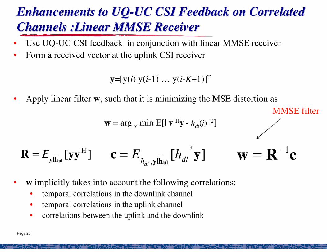
Enhancements to UQEnhancements to UQ--UC CSI Feedback on Correlated UC CSI Feedback on Correlated Channels :Linear MMSE ReceiverChannels :Linear MMSE Receiver

• Use UQ-UC CSI feedback in conjunction with linear MMSE receiver• Form a received vector at the uplink CSI receiver

y=[y(i) y(i-1) … y(i-K+1)]T

• Apply linear filter w, such that it is minimizing the MSE distortion as

w = arg v min E[| v Hy - hdl(i) |2]

• w implicitly takes into account the following correlations:• temporal correlations in the downlink channel• temporal correlations in the uplink channel• correlations between the uplink and the downlink

][ HyyRulh|yE= ][ *

,yc

ulh|y dlhhE

dl= cRw 1−=

MMSE filter

Page:21

MSE Distortion PerformanceMSE Distortion Performance• Downlink channel is modeled as an ARMA process whose coefficients are chosen to

correspond to Jake's model for a carrier frequency of 2GHz and different mobile terminal velocities

dB10log10 =���

����

�=

o

csiulcsi

ul NP

SNRv =10kmph

Page:22

UQUQ--UC CSI Feedback for ZF Spatial PreUC CSI Feedback for ZF Spatial Pre--FilteringFiltering• Base station obtains CSI

corresponding to each downlink channel state hnm

• CSI is obtained from each mobile terminal using the UQ-UC CSI feedback

• At time instant i, terminal n (n=1, …, N) is transmitting the corresponding CSI hnm(i) via the uplink CSI feedback channel

• Instead of the ideal channel state hnm(i), the spatial pre-filter applies the estimate of hnm(i) obtained from the uplink CSI feedback receiver

•

Page:23

ConclusionConclusion• Transmitter optimization schemes were presented

• MMSE prediction described showing its effectiveness

• We presented the ‘zero-delay’ UQ-UC CSI feedback scheme on correlated wireless channels

• ‘Zero-delay’ UQ-UC CSI feedback optimal for mutually independent iidRayleigh downlink and AWGN uplink

• We described the ARMA correlated channel model and presented thecorresponding performance bounds for the UQ-UC CSI feedback scheme

• Performance limits of the scheme in the context of downlink multiple antenna multiuser transmitter optimization

• Attractive choice for CSI feedback

Page:24

Future DirectionsFuture Directions• Transmitter optimization with delayed CSI

• TDD uplink/downlink multiplexing • Environments that offer narrow angular spread should be considered

because they may allow a base station to obtain downlink CSI without explicit feedback from a mobile terminal

• Channel state prediction schemes -validation using real propagation measurements may be of interest

• UQ-UC CSI feedback scheme • Understanding the trade-off between resources (e.g., power, time and

spectrum) allocated to the pilots and the CSI feedback versus the resources of the data carrying signals on the downlink and

• To compare the presented UQ-UC CSI feedback scheme to different schemes that use quantization and channel coding optimized for a given delay constraint