Channel Estimation for Mobile Wideband Code DivisionMultiple Access (WCDMA)

Von der Fakultät Informatik, Elektrotechnik und Informationstechnikder Universität Stuttgart zur Erlangung der Würde einesDoktor-Ingenieurs (Dr.-Ing.) genehmigte Abhandlung

Vorgelegt von

Stephan Saur

aus Stuttgart

Hauptberichter: Prof. Dr.-Ing. J. SpeidelMitberichter: Prof. Dr.-Ing. N. FrühaufTag der mündlichen Prüfung: 7. Januar 2008

Institut für Nachrichtenübertragung der Universität Stuttgart

2008

The dissertation at hand evolved from my research and teaching activities at the Institute ofTelecommunications, University of Stuttgart, Germany.

Special thanks go to my professor, Dr.-Ing. Joachim Speidel, for giving me the opportunityto work under his supervision. Numerous profitable discussions and suggestions have lastingcontributed to the success of this work.

Also, I cordially thank Prof. Dr.-Ing. Norbert Frühauf for taking over the assessment of thisthesis.

I express my sincere gratitude to Dr.-Ing. Volker Braun and his colleagues at Alcatel-LucentBell Labs in Stuttgart for the motivation and their considerate support during my participa-tion in a research cooperation.

I am grateful to all colleagues at the Institute of Telecommunications, especially Dr.-Ing. Hanns Thilo Hagmeyer, for fruitful discussions and their backing. They were alwaysopen for questions and encouraged my research work.

Moreover, I would like to thank all students who I was workingwith during the past yearsfor their engagement.

Special thanks also go to my family and friends who contributed with manifold support tothe work at hand.

Contents

Acronyms ix

Notation xi

Abstract xvii

Kurzfassung xvii

1 Introduction 1

2 The Universal Mobile Telecommunications System (UMTS) 3

2.1 Architecture overview . . . . . . . . . . . . . . . . . . . . . . . . . . . .. 3

2.2 The physical layer - general description . . . . . . . . . . . . .. . . . . . 4

2.3 Physical layer transmitter . . . . . . . . . . . . . . . . . . . . . . . .. . . 5

2.3.1 Bit processing . . . . . . . . . . . . . . . . . . . . . . . . . . . . 6

2.3.2 Spreading and modulation . . . . . . . . . . . . . . . . . . . . . . 9

2.4 The mobile radio channel . . . . . . . . . . . . . . . . . . . . . . . . . . .14

2.5 Physical layer receiver . . . . . . . . . . . . . . . . . . . . . . . . . . .. 17

2.5.1 Finger detector . . . . . . . . . . . . . . . . . . . . . . . . . . . . 19

2.5.2 Despreader . . . . . . . . . . . . . . . . . . . . . . . . . . . . . . 23

2.5.3 Simplified system model . . . . . . . . . . . . . . . . . . . . . . . 25

2.5.4 Channel estimator and maximum ratio combiner . . . . . . .. . . 28

2.5.5 Sample processing . . . . . . . . . . . . . . . . . . . . . . . . . . 30

vii

3 Channel estimation without feedback 33

3.1 Weighted multi-slot averaging (WMSA) . . . . . . . . . . . . . . .. . . . 35

3.1.1 The basic principle . . . . . . . . . . . . . . . . . . . . . . . . . . 35

3.1.2 Optimizing the weighting vector . . . . . . . . . . . . . . . . . .. 38

3.2 Moving average (MA) . . . . . . . . . . . . . . . . . . . . . . . . . . . . 41

3.3 WMSA and moving average with interpolation . . . . . . . . . . .. . . . 45

3.4 BER and BLER performance evaluation . . . . . . . . . . . . . . . . .. . 47

4 Channel estimation with rake feedback 55

4.1 DPCCH rake feedback . . . . . . . . . . . . . . . . . . . . . . . . . . . . 55

4.2 DPDCH rake feedback . . . . . . . . . . . . . . . . . . . . . . . . . . . . 59

4.3 Concatenation of DPCCH- and DPDCH rake feedback . . . . . . .. . . . 62

4.4 Simulation results . . . . . . . . . . . . . . . . . . . . . . . . . . . . . . .64

5 Channel estimation with decoder feedback 69

5.1 The receiver with decoder feedback . . . . . . . . . . . . . . . . . .. . . 69

5.2 Parameter optimization . . . . . . . . . . . . . . . . . . . . . . . . . . .. 73

5.3 Simulation results . . . . . . . . . . . . . . . . . . . . . . . . . . . . . . .77

6 Velocity estimation 85

6.1 Estimation in the frequency domain . . . . . . . . . . . . . . . . . .. . . 85

6.2 Velocity classes and parameter optimization . . . . . . . . .. . . . . . . . 87

6.3 Adaptive channel estimation . . . . . . . . . . . . . . . . . . . . . . .. . 93

6.4 Alternative approach - velocity estimation in the time domain . . . . . . . . 94

7 Conclusion 97

A Bit processing example 99

B Simulation parameters 100

B.1 System parameters . . . . . . . . . . . . . . . . . . . . . . . . . . . . . . 100

B.2 Mobile radio channel parameters . . . . . . . . . . . . . . . . . . . .. . . 101

B.3 Receiver parameters . . . . . . . . . . . . . . . . . . . . . . . . . . . . . .101

viii

Acronyms

3GPP third generation partnership projectAWGN additive white Gaussian noiseBER bit error ratioBLER block error ratioCDMA code division multiple accessCE channel estimationCN core networkCRC cyclic redundancy checkCRLB Cramer-Rao lower boundCSD circuit switched dataDPCCH dedicated physical control channelDPDCH dedicated physical data channelEGC equal gain combiningFBI feedback informationFDD frequency division duplexFDMA frequency division multiple accessGPRS general packet radio serviceGSM global system for mobile communications

formerly: groupe spécial mobileHPSK hybrid phase shift keyingHSCSD high-speed circuit switched dataHSDPA high-speed downlink packet accessIMT international mobile telecommunicationsLOS line of sightLTE long-term evolutionMA moving averageMA-I moving average with interpolationMAC medium access controlMCI multi-code interferenceMIMO multiple input multiple outputMRC maximum ratio combinerMUI multi-user interferenceOVSF orthogonal variable spreading factor

ix

QPSK quadrature phase shift keyingRNC radio network controllerSD selection diversitySISO soft-in soft-outSNR signal-to-noise ratioTDD time division duplexTDMA time division multiple accessTFCI transport format combination indicatorTPC transmit power controlTTI transmission time intervalUE user equipmentUMTS universal mobile telecommunications systemUTRA UMTS terrestrial radio accessUTRAN UMTS terrestrial radio access networkWCDMA wideband CDMAWMSA weighted multi-slot averagingWMSA-I weighted multi-slot averaging with interpolationWSSUS wide-sense stationary uncorrelated scattering

x

Notation

−• Fourier transform•− inverse Fourier transform⋆ convolution⊕ modulo 2 addition⌊x⌋ greatest integer smaller than or equal tox⌈x⌉ smallest integer greater than or equal toxx∗ conjugate complex ofxx estimate ofx|x| absolute value ofxxn mean value of samplesxn

xk input to the decoder ifxk is output from the coderx′k bitsxk permuted by the turbo coder interleaverxC variablex related to the DPCCHxD variablex related to the DPDCHxMA variablex related to the moving average algorithmxMA-I variablex related to the moving average algorithm with interpolationxWMSA variablex related to the WMSA algorithmxWMSA-I variablex related to the WMSA algorithm with interpolationarcx phase ofxargmaxf (x) valuex corresponding to the global maximum off (x)D delay operatorE[x] expectation ofxf (x) function of variablexℑx imaginary part ofxmax(xn) maximum of all valuesxn

mod(x,y) remainder of the integer divisionx/yP[x] probability of eventxpx (x) probability density function of random variablexQxx(k) autocorrelation function ofxn

ℜx real part ofx

A number of receive antennasATPC amplification factor due to transmit power control

xi

a receive antenna indexaC

n finger combined samples of the DPCCHaµ,m, aD

µ,m finger combined samples of DPDCHµB despreading scaling factorBν number of bits per block of the transport channelνb(τ, t) bandpass channel impulse responsebν,k sent bit sequence of the transport channelνc speed of lightc discrete-time index in chip clockcν code rate of the transport channelνd0 finger detection decision thresholdda,ξ stepwise added descrambled samples ˜oa,ξ ,h used for finger detectiondl mean attenuation of fingerlEb received energy per information bit per antennael ,m channel estimation error of fingerlf frequencyf0 carrier frequencyfB signal bandwidthfDr (t) , fDr Doppler frequency of pathrfD,max maximal Doppler frequencyfOS oversampling frequencyg(t)−•G(ω) pulse shaping filterH1 delay of first received path in half-chip intervalsHC

b multiple of the DPCCH bit interval in half-chip intervalsHf frame duration in half-chip intervalsHs maximal delay that can be detected in half-chip intervalsh discrete-time index in half-chip clockh(τ, t) equivalent lowpass channel impulse responsehl (t) fading sequence of fingerlhl (τ, t) equivalent lowpass channel impulse response with respect to fingerlhl ,m, h′l ,n fading channel coefficient of fingerl

I WMSA filter lengthIP number of DPDCHs in the I-branchIT number of turbo decoder iterationsi slot indexJ number of frames per TTIj imaginary unitK code block lengthk discrete-time index in bit clockkC

c DPCCH channelization (spreading) codekD

µ,c channelization (spreading) code of the DPDCHµL number of rake fingers

xii

L12,k, L21,k input and output L-values of the SISO decodersLch channel L-valueLk L-value of samplekLthr L-value threshold used for decoder feedbackl rake finger indexM number of bits per DPDCH slotM′ number of DPDCH bits per DPCCH bit intervalMOS oversampling factorMP number of physical channels (DPDCHs)Mκ number of information bits in slotκm discrete-time index in DPDCH bit clockN number of bits per DPCCH slotN0 one-sided noise power spectral densityNA number of compensated pilot samples used for averagingNF effective length of the extended training sequenceNFBI number of FBI bits per slotNP number of pilot bits per slotNT number of transport channelsNTFCI number of TFCI bits per slotNTPC number of TPC bits per slotn discrete-time index in DPCCH bit clockn(t) lowpass noisen(t) bandpass noisenl ,µ,m sampled noise of DPDCHµ and fingerln′l ,n sampled noise of fingerlnµ,m noise samples after finger combiningol ,c samples of fingerl in chip clockoa,ξ ,h delayed and descrambled samples of the finger detector branch ξo′l ,h samples of fingerl in half-chip clock

Pl ,m instantaneous received signal power of fingerlPn present time equivalent for samplenQP number of DPDCHs in the Q-branchqa(t) baseband signal received at antennaaqa,h samples of signalqa(t) received at antennaaR number of pathsRc scrambling code in chip clockRh scrambling code in half-chip clockr path indexrc channel bit rater id (t)−•Rid

(

f)

ideal lowpassrCl ,n received DPCCH samples of fingerl

rDl ,µ,m received samples of DPDCHµ and fingerl

xiii

rν information bit rate of the transport channelνS spreading factorsCn sent DPCCH bit sequence

s′Cc DPCCH chip sequence before channelizationsD

µ,m sent bit sequence of the DPDCHµs′Dµ,c chip sequence of the DPDCHµ before channelizationT termination bit vector of the turbo coder, part ofYTC

b DPCCH bit intervalTc chip intervalTf frame durationTOS oversampling clockTobs channel observation timeTslot slot durationTν number of blocks per TTI of the transport channelνt timeTκ,ν moving average time stamp for compensated pilot sampleχκ,νu(t) sent radio frequency signalv, vi velocity of the mobile terminal during slotiv′i instantaneous velocity estimate for slotiw(t) response ofh(τ, t) to the sent baseband signalx(t)w WMSA weighting vectorwv WMSA weighting vector optimized for velocityvwκ WMSA weighting factor for slotκwκ,ν,n moving average weighting factor for sampleν in slot κX input block to the coderXκ power spectrum ofχn

x(t) sent baseband signalxc scrambled chip sequencex′c chip sequence before scramblingxk input bits to the coder, elements ofXY output block from the coderya(t) radio frequency signal received at antennaayk output bits from the turbo coder, elements ofYZ number of multipath tapsz multipath tap indexz0,k, z1,k, z2,k output bits from the convolutional coder, elements ofYzk output bits from the turbo coder, elements ofYα roll-off factorαl ,r angle of arrival of pathr in finger lβ physical channel amplification factorΓC

i,n extended training sequence based on fed back DPCCH non-pilot samplesaC

i,n

xiv

ΓDi,m extended training sequence based on fed back DPDCH samplesaD

i,m

γ DPCCH-to-DPDCH-power ratio∆κ,ν,n time offset between sloti, samplen and slotκ , sampleν∆vi velocity estimation error∆φi phase rotation betweenhi−1 andhi

δ (t) Dirac impulseε received signal envelopeζ rake feedback and decoder feedback scaling factorη weighting factor used for velocity estimationκ slot indexΛ length of a vector used for velocity estimationλ signal wavelengthµ DPDCH indexν transport channel indexν discrete-time index in DPCCH bit clockξ branch index of the finger detectorπ Archimedes’ constantρν puncturing limit of the transport channelνσ2 mean received signal powerσ2

a noise power after finger combiningσ2

C noise power on DPCCH after despreadingσ2

D noise power on DPDCH after despreadingσ2

e noise power due to channel estimation errorτ timeτmax maximal possible path delay that allows for finger detectionτr , τr (t) delay of pathrϒ norming factor for DPDCH rake feedback and decoder feedbackΦl ,r random phase shift of pathr in finger lφc phase shift due to scramblingϕi,m channel estimation phase error of DPDCH samplem in slot iχn compensated pilot sampleχκ instantaneous channel estimate of slotκψ rake feedback threshold angleΩ moving average target filter lengthΩv moving average target filter length optimized for velocityvΩ′

n sum of all moving average weighting factorswκ,ν,n

special casewκ,ν,n ∈ 0,1: moving average filter length depending onindexn

ω angular frequencyω0 carrier angular frequency

xv

AbstractThe mobile radio standard UMTS uses wideband code division multiple access (WCDMA)for the transmission of data and control information of the subscribers. The major part of thecontrol information consists of pilot bits that allow the estimation of the time-variant channelimpulse response at the receiver. Without channel estimation data cannot be detected. Thebasic estimation method is averaging the pilots in order to reduce noise on the estimates.In particular if the mobile subscriber moves with high speed, estimation represents a severechallenge for the receiver due to the strong time-variance of the channel. In the work at hand,firstly, the two basic algorithms weighted multi-slot averaging (WMSA) and moving averageare presented and investigated for this matter. As possibleextension an interpolation schemeis discussed. The following chapters deal with methods which reduce the data block errorratio (BLER) by feeding the already detected data back to thechannel estimator. We distin-guish thereby between feedback inside the rake receiver (rake feedback) and feedback afterthe decoder (decoder feedback). Finally, an algorithm is described that estimates the velocityof the mobile subscriber. It allows for an adaptation of the channel estimation parametersand thus for a further improvement of the receiver.

KurzfassungDer Mobilfunkstandard UMTS verwendet das Wideband Code Division Multiple Access(WCDMA) Verfahren zur Übertragung von Daten und Steuerinformationen der Teilnehmer.Ein wesentlicher Teil der Steuerinformation sind Pilotbits, die im Empfänger zur Schät-zung der zeitvarianten Kanalimpulsantwort dienen. Ohne Kanalschätzung können die Datennicht detektiert werden. Das einfachste Schätzverfahren ist eine Mittelung empfangenerPilote, um das Rauschen der Schätzwerte zu reduzieren. Insbesondere wenn sich der Mobil-funkteilnehmer mit hoher Geschwindigkeit bewegt, stellt die Schätzung wegen der starkenZeitvarianz des Mobilfunkkanals eine große Herausforderung für den Empfänger dar. Indieser Arbeit werden dafür zunächst die zwei grundlegendenAlgorithmen Weighted Multi-Slot Averaging (WMSA) und Moving Average vorgestellt und untersucht. Als möglicheErweiterung wird ein Interpolationsverfahren diskutiert. Die folgenden Kapitel beschäftigensich mit Methoden, die durch Rückkopplung der bereits detektierten Daten in den Kanal-schätzer die Fehlerhäufigkeit der Datenblöcke (BLER) reduzieren. Dabei wird zwischender Rückkopplung innerhalb des Rake Empfängers (Rake Feedback) und der Rückkopplungnach dem Decoder (Decoder Feedback) unterschieden. Abschließend wird ein Algorith-mus zur Schätzung der Geschwindigkeit des Mobilfunkteilnehmers beschrieben. Dieser er-möglicht eine Anpassung der Kanalschätzparameter und somit eine weitere Verbesserungdes Empfängers.

xvii

Chapter 1

Introduction

Mobile radio has experienced a tremendous worldwide growthduring the past years. Im-proved modulation and coding techniques, advances in semiconductor technologies and fi-nally a better knowledge of the mobile radio channel have sustainably contributed to thisevolution.

The age of mobile radio in Germany started in 1926 when the first serviceable system wasbuilt up for public transportation. The so-called first generation of area-wide mobile radiosystems for everyone was still based on analog technique [1]. Its commencements date backalmost fifty years. However, the user had to know where his dialog partner was situated. Thefirst cellular network in Germany was launched in 1985. For the first time it was possible todetermine the position of a user. The handover from cell to cell happened automatically.

In the early 1990s years second generation systems were established which used digital radiotechnology for the first time. The Global System for Mobile Communications (GSM) is itsmost prominent representative. It was designed for the transmission of speech and exhibits amaximal bit rate of 9.6kbit/s [2]. GSM utilizes the time division multiple access (TDMA)and the frequency division multiple access (FDMA) techniques to assign one particular chan-nel to one user. This is referred to as circuit switched data (CSD) transmission.

As sophisticated applications like mobile internet or video communications require morebandwidth, some enhancements came into existence. Important examples are the high-speedcircuit switched data (HSCSD) system that bundles several GSM channels, and the GeneralPacket Radio Service (GPRS) [2], which allocates momentarily available time-slots and thusrepresents a packet based transmission. Although GPRS provides more than 100kbit/s bitrate, it will not be able to face the challenges of the future.

Therefore, a third generation of mobile radio is developed by the Third Generation Partner-ship Project (3GPP) [3]. It is commonly denoted as UniversalMobile TelecommunicationsSystem (UMTS) in Europe and as International Mobile Telecommunications 2000 (IMT2000) worldwide. In contrast to previous systems, it is based on the code division multi-ple access (CDMA) technique where several users transmit atthe same time with the same

1

carrier frequency. Since its introduction in recent years it becomes more and more popu-lar. The primary architecture of UMTS, often named as Release 99, provides bit rates upto 2Mbit/s. However, enhancements will increase this value significantly, e.g. high-speeddownlink packet access (HSDPA) and 3G long-term evolution (LTE). The latter will multiplythe spectral efficiency by using multiple input multiple output (MIMO) antennas.

With an increasing number of users and higher bit rates also the requirements for mobileterminals and base stations become continuously more specific. Among the receiver func-tions, channel estimation represents an outstanding position. Due to scattering and movingsubscribers, the impulse response of the mobile radio channel becomes time-variant. Chan-nel estimation has to cope with multipath fading. A rake receiver detects separable paths,so-called fingers, which are represented by time-variant complex channel coefficients. Esti-mates of these coefficients enable combining and decoding ofthe finger signals. The disser-tation at hand describes and compares several channel estimation strategies.

First of all, Chapter 2 deals with the transmission system. After a brief overview of thesystem architecture of UMTS, the physical layer is described in detail. Transmitter functions,e.g. channel coding, spreading and modulation, are specified in [4] and [5]. Only those partsthat are necessary for the later understanding are presented. After the description of the time-variant mobile radio channel model, the respective receiver is discussed. It has to mitigatethe impairments caused by the channel and to invert the related transmitter functions.

Chapter 3 concentrates on channel estimation based on the received pilot samples. Startingfrom the basic principle of averaging over a set of received pilots, several implementationsare discussed and compared. The sensitivity of the parameters to noise and fading is shown.Optimized parameters are presented for selected velocities of the mobile terminal.

In Chapter 4, a feedback loop within the rake receiver is established. After a first channelestimation based on received pilots only, finger combined data samples are fed back andutilized as extended training sequence for a second improved channel estimation. Also thisrake feedback allows several options that are investigatedand evaluated.

A further receiver design is presented in Chapter 5. Now, thefeedback loop is applied afterthe decoder that provides reliability information about its output. This knowledge can beexploited by the channel estimator, which on his part allowsfor improved data samples atthe decoder input, thus reducing the bit error ratio (BER). Several implementation optionsare discussed. As both pilot and data samples are utilized for channel estimation, also theoptimization of system parameters, e.g. the power portion of the pilots, have to be taken intoconsideration.

As the optimal channel estimation parameters strongly depend on the velocity of the mobilesubscriber, a method for estimating the velocity is proposed in Chapter 6. The receivedpilot samples are thereby evaluated in the frequency domain. The improved receiver withoutfeedback loop, which adapts to the instantaneous channel conditions, is compared to theconventional method from Chapter 3.

The most important results are finally summarized in Chapter7.

2

Chapter 2

The Universal MobileTelecommunications System (UMTS)

2.1 Architecture overview

At first, a brief overview of the architecture of UMTS shall help to classify the work athand within the complex world of 3GPP. Figure 2.1 shows that the considered mobile radiosystem consists of three domains, namely mobile terminals (user equipment, UE), the ac-cess network (UMTS terrestrial radio access network, UTRAN) and the core network (CN).The interface between UE and UTRAN is calledUu-interface and characterizes the radiotransmission between mobile terminal and base station (Node B). TheIu-interface betweenUTRAN and CN is separated intoIuCS for circuit switched transmission andIuPS that pro-vides a link to the packet switching network. The componentsof the CN are not itemizedhere. The interested reader is referred to [6, 7]. The CN was adopted to a large extent fromthe second generation, whereas the UTRAN and the UE had to be fully redesigned [8].

The UTRAN is separated into sub-networks. Each sub-networkis managed by a radio net-work controller (RNC) and consists of several base stationswhich provide the resources forone or more cells. UMTS supports a hierarchy of supply areas.Three types of cells can bedistinguished. Macro cells have a large radius of more than 1km and provide a basic networkcoverage, whereas micro cells improve the supply in urban and suburban areas. Finally, picocells are designed for indoor communications, e.g. at airports or railway stations, where a lotof people may dial in.

In the following, we consider only the physical layer of the radio interfaceUu in uplinkdirection, i.e. the transmitter is a mobile terminal that moves in the general case with acertain velocityv, and the receiver is a base station. Moreover, we assume a single user andsingle cell system. Interference and handover effects are not subject of the work at hand.

3

UE

UE

radiocell

Uu

-

-

UTRAN

Node B - RNC -

]

^

UTRAN

Node B

R

I

Node B

RNC

-

Iu

CN

circuitswitchednetwork

environment

packet

switchednetwork

environment

Figure 2.1: The most important components of the UMTS architecture

2.2 The physical layer - general description

The system under consideration operates in frequency division duplex (FDD) mode, whereuplink and downlink use different frequency bands that havea specified separation dis-tance [9]. Also a time division duplex (TDD) mode is defined. It provides a commonfrequency band and synchronized time intervals for uplink and downlink traffic. The trans-mission system operates with code division multiple access(CDMA). Due to the spreadsignal bandwidth of approximatelyfB = 5MHz, it is often referred to as wideband CDMA(WCDMA).

The physical layer offers data transport services to the medium access control (MAC) layer.The access to these services is carried out by the use of transport channels. There are severaltypes of dedicated and common transport channels [10]. Theyare mapped to various types ofphysical channels that at last realize the physical layer data transmission. In the following,we will consider only two types of physical channels, namelythe dedicated physical datachannel (DPDCH) and the dedicated physical control channel(DPCCH), which we will getto know in more detail.

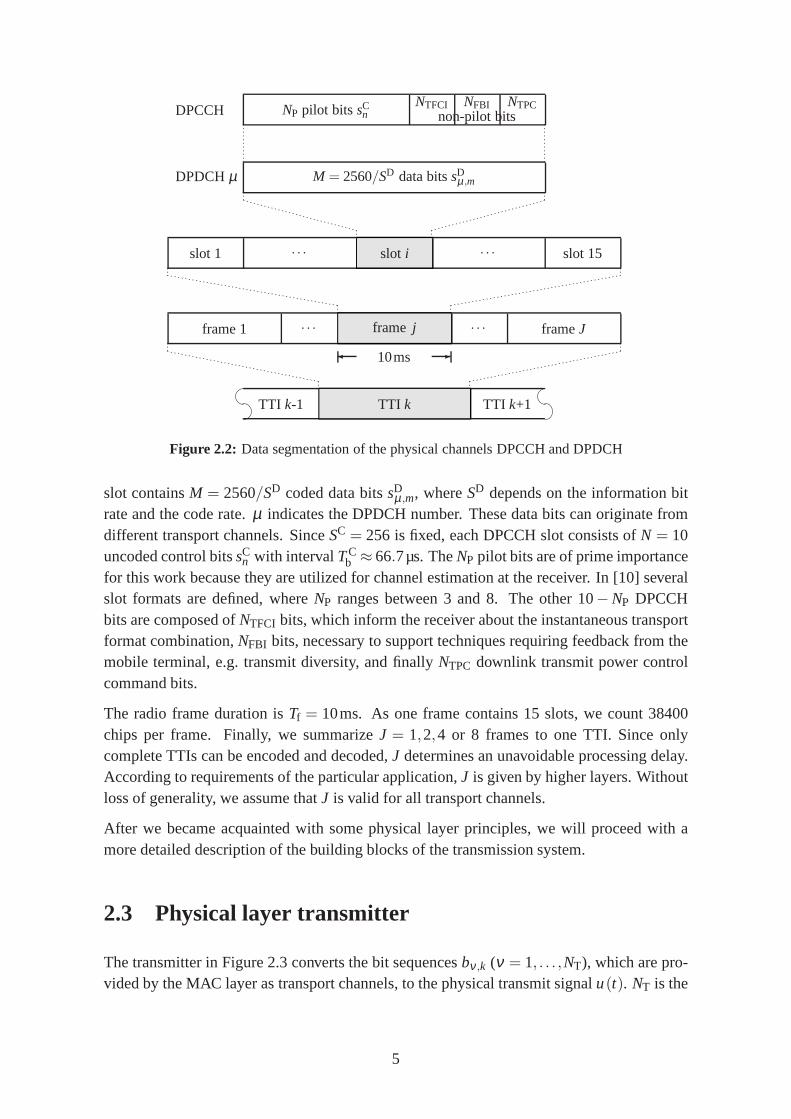
According to Figure 2.2, both DPDCH and DPCCH are segmented into slots, frames andtransmission time intervals (TTIs). The slot duration isTslot≈ 666.7µs, and each slot consistsof 2560 chipsxc with the intervalTc ≈ 260ns. One slot corresponds, depending on thespreading factorsSD (DPDCH) andSC (DPCCH), to a certain number of bits. The DPDCH

4

DPCCH NP pilot bits sCn

NTFCI NFBI NTPCnon-pilot bits

DPDCHµ M = 2560/SD data bitssDµ ,m

slot 1 · · · slot i · · · slot 15

frame 1 · · · frame j · · · frameJ

-10ms

TTI k-1 TTI k TTI k+1

Figure 2.2: Data segmentation of the physical channels DPCCH and DPDCH

slot containsM = 2560/SD coded data bitssDµ,m, whereSD depends on the information bit

rate and the code rate.µ indicates the DPDCH number. These data bits can originate fromdifferent transport channels. SinceSC = 256 is fixed, each DPCCH slot consists ofN = 10uncoded control bitssC

n with intervalTCb ≈ 66.7µs. TheNP pilot bits are of prime importance

for this work because they are utilized for channel estimation at the receiver. In [10] severalslot formats are defined, whereNP ranges between 3 and 8. The other 10−NP DPCCHbits are composed ofNTFCI bits, which inform the receiver about the instantaneous transportformat combination,NFBI bits, necessary to support techniques requiring feedback from themobile terminal, e.g. transmit diversity, and finallyNTPC downlink transmit power controlcommand bits.

The radio frame duration isTf = 10ms. As one frame contains 15 slots, we count 38400chips per frame. Finally, we summarizeJ = 1,2,4 or 8 frames to one TTI. Since onlycomplete TTIs can be encoded and decoded,J determines an unavoidable processing delay.According to requirements of the particular application,J is given by higher layers. Withoutloss of generality, we assume thatJ is valid for all transport channels.

After we became acquainted with some physical layer principles, we will proceed with amore detailed description of the building blocks of the transmission system.

2.3 Physical layer transmitter

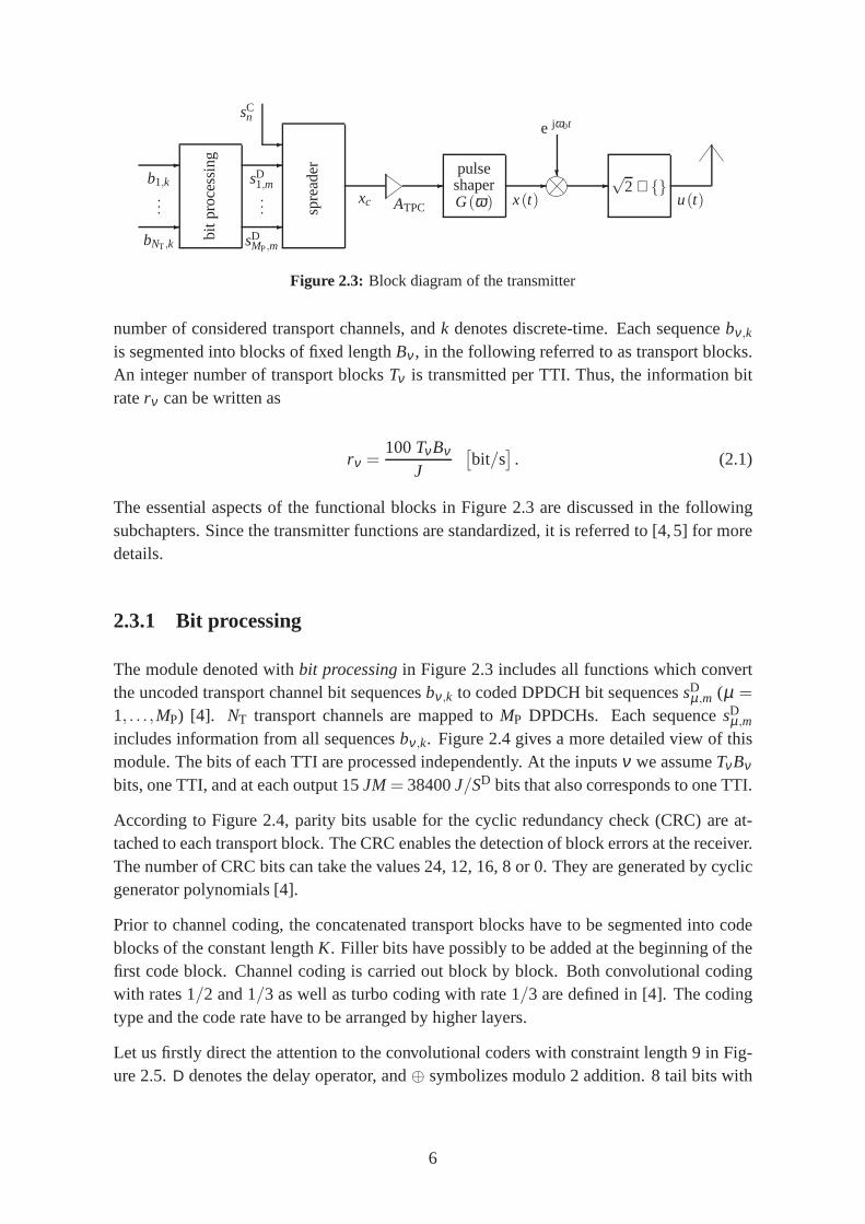
The transmitter in Figure 2.3 converts the bit sequencesbν,k (ν = 1, . . . ,NT), which are pro-vided by the MAC layer as transport channels, to the physicaltransmit signalu(t). NT is the

5

bitp

roce

ssin

g-

bNT ,k

-b1,k

···

-sDMP,m

-sD1,m

···

sCn

-

spre

ader

xc ATPC

-pulseshaperG(ω)

-x(t)

-?

e jω0t

√2 ℜ

u(t)

Figure 2.3: Block diagram of the transmitter

number of considered transport channels, andk denotes discrete-time. Each sequencebν,k

is segmented into blocks of fixed lengthBν , in the following referred to as transport blocks.An integer number of transport blocksTν is transmitted per TTI. Thus, the information bitraterν can be written as

rν =100TνBν

J

[

bit/s]

. (2.1)

The essential aspects of the functional blocks in Figure 2.3are discussed in the followingsubchapters. Since the transmitter functions are standardized, it is referred to [4,5] for moredetails.

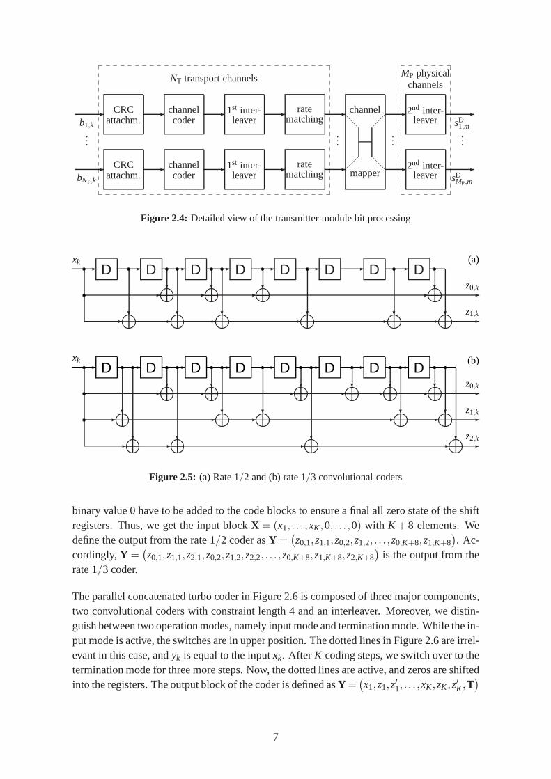
2.3.1 Bit processing

The module denoted withbit processingin Figure 2.3 includes all functions which convertthe uncoded transport channel bit sequencesbν,k to coded DPDCH bit sequencessD

µ,m (µ =

1, . . . ,MP) [4]. NT transport channels are mapped toMP DPDCHs. Each sequencesDµ,m

includes information from all sequencesbν,k. Figure 2.4 gives a more detailed view of thismodule. The bits of each TTI are processed independently. Atthe inputsν we assumeTνBνbits, one TTI, and at each output 15JM = 38400J/SD bits that also corresponds to one TTI.

According to Figure 2.4, parity bits usable for the cyclic redundancy check (CRC) are at-tached to each transport block. The CRC enables the detection of block errors at the receiver.The number of CRC bits can take the values 24, 12, 16, 8 or 0. They are generated by cyclicgenerator polynomials [4].

Prior to channel coding, the concatenated transport blockshave to be segmented into codeblocks of the constant lengthK. Filler bits have possibly to be added at the beginning of thefirst code block. Channel coding is carried out block by block. Both convolutional codingwith rates 1/2 and 1/3 as well as turbo coding with rate 1/3 are defined in [4]. The codingtype and the code rate have to be arranged by higher layers.

Let us firstly direct the attention to the convolutional coders with constraint length 9 in Fig-ure 2.5.D denotes the delay operator, and⊕ symbolizes modulo 2 addition. 8 tail bits with

6

NT transport channels

-bNT ,k

CRCattachm.

-

-b1,k

CRCattachm.

-

···

channelcoder

-

channelcoder

-

1st inter-leaver

-

1st inter-leaver

-

ratematching

-

ratematching

-

···

channel

mapper-

-

···

MP physicalchannels

2nd inter-leaver

-sDMP,m

2nd inter-leaver

-sD1,m

···

Figure 2.4: Detailed view of the transmitter module bit processing

D D D D D D D D- - - - - - - -

? ? ? ?

? ? ? ? ? ?

- - - - -

- - - - - - -

xk

z0,k

z1,k

(a)

D D D D D D D D- - - - - - - -

? ? ? ? ? ?

? ? ? ? ?

? ? ? ?

- - - - - - -

- - - - - -

- - - - -

xk

z0,k

z1,k

z2,k

(b)

Figure 2.5: (a) Rate 1/2 and (b) rate 1/3 convolutional coders

binary value 0 have to be added to the code blocks to ensure a final all zero state of the shiftregisters. Thus, we get the input blockX = (x1, . . . ,xK,0, . . . ,0) with K + 8 elements. Wedefine the output from the rate 1/2 coder asY =

(

z0,1,z1,1,z0,2,z1,2, . . . ,z0,K+8,z1,K+8)

. Ac-cordingly,Y =

(

z0,1,z1,1,z2,1,z0,2,z1,2,z2,2, . . . ,z0,K+8,z1,K+8,z2,K+8)

is the output from therate 1/3 coder.

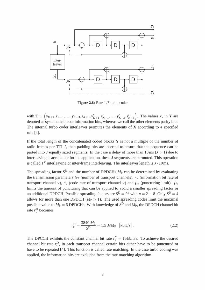
The parallel concatenated turbo coder in Figure 2.6 is composed of three major components,two convolutional coders with constraint length 4 and an interleaver. Moreover, we distin-guish between two operation modes, namely input mode and termination mode. While the in-put mode is active, the switches are in upper position. The dotted lines in Figure 2.6 are irrel-evant in this case, andyk is equal to the inputxk. After K coding steps, we switch over to thetermination mode for three more steps. Now, the dotted linesare active, and zeros are shiftedinto the registers. The output block of the coder is defined asY =

(

x1,z1,z′1, . . . ,xK,zK,z′K,T)

7

xk

inter-leaver

?

x′k

D D D- - - -

- - -

6 6

?6

6

-

-yk

zk

D D D- - - -

- - -

6 6

?6

6

-

-

z′k

y′k

Figure 2.6: Rate 1/3 turbo coder

with T =(

yK+1,zK+1, . . . ,yK+3,zK+3,y′K+1,z′K+1, . . . ,y

′K+3,z

′K+3

)

. The valuesxk in Y aredenoted as systematic bits or information bits, whereas we call the other elements parity bits.The internal turbo coder interleaver permutes the elementsof X according to a specifiedrule [4].

If the total length of the concatenated coded blocksY is not a multiple of the number ofradio frames per TTIJ, then padding bits are inserted to ensure that the sequence can beparted intoJ equally sized segments. In the case a delay of more than 10ms (J > 1) due tointerleaving is acceptable for the application, theseJ segments are permuted. This operationis called 1st interleaving or inter-frame interleaving. The interleaver length isJ ·10ms.

The spreading factorSD and the number of DPDCHsMP can be determined by evaluatingthe transmission parametersNT (number of transport channels),rν (information bit rate oftransport channelν), cν (code rate of transport channelν) andρν (puncturing limit). ρνlimits the amount of puncturing that can be applied to avoid asmaller spreading factor oran additional DPDCH. Possible spreading factors areSD = 2n with n = 2· · ·8. OnlySD = 4allows for more than one DPDCH (MP > 1). The used spreading codes limit the maximalpossible value toMP = 6 DPDCHs. With knowledge ofSD andMP, the DPDCH channel bitraterD

c becomes

rDc =

3840MP

SD = 1.5 MMP[

kbit/s]

. (2.2)

The DPCCH exhibits the constant channel bit raterCc = 15kbit/s. To achieve the desired

channel bit raterDc , in each transport channel certain bits either have to be punctured or

have to be repeated [4]. This function is called rate matching. In the case turbo coding wasapplied, the information bits are excluded from the rate matching algorithm.

8

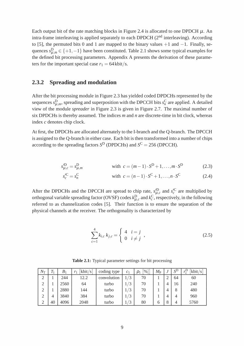
Each output bit of the rate matching blocks in Figure 2.4 is allocated to one DPDCHµ. Anintra-frame interleaving is applied separately to each DPDCH (2nd interleaving). Accordingto [5], the permuted bits 0 and 1 are mapped to the binary values +1 and−1. Finally, se-quencessD

µ,m∈ +1,−1 have been constituted. Table 2.1 shows some typical examples forthe defined bit processing parameters. Appendix A presents the derivation of these parame-ters for the important special caser1 = 64kbit/s.

2.3.2 Spreading and modulation

After the bit processing module in Figure 2.3 has yielded coded DPDCHs represented by thesequencessD

µ,m, spreading and superposition with the DPCCH bitssCn are applied. A detailed

view of the modulespreaderin Figure 2.3 is given in Figure 2.7. The maximal number ofsix DPDCHs is thereby assumed. The indicesmandn are discrete-time in bit clock, whereasindexc denotes chip clock.

At first, the DPDCHs are allocated alternately to the I-branch and the Q-branch. The DPCCHis assigned to the Q-branch in either case. Each bit is then transformed into a number of chipsaccording to the spreading factorsSD (DPDCHs) andSC = 256 (DPCCH).

s′Dµ,c = sDµ,m with c = (m−1) ·SD +1, . . . ,m·SD (2.3)

s′Cc = sCn with c = (n−1) ·SC+1, . . . ,n ·SC (2.4)

After the DPDCHs and the DPCCH are spread to chip rate,s′Dµ,c ands′Cc are multiplied byorthogonal variable spreading factor (OVSF) codeskD

µ,c andkCc , respectively, in the following

referred to as channelization codes [5]. Their function is to ensure the separation of thephysical channels at the receiver. The orthogonality is characterized by

4∑

c=1

ki,c k j ,c =

4 i = j0 i 6= j

, (2.5)

Table 2.1: Typical parameter settings for bit processing

NT T1 B1 r1[

kbit/s]

coding type c1 ρ1[

%]]

MP J SD rDc

[

kbit/s]

2 1 244 12.2 convolution 1/3 70 1 2 64 602 1 2560 64 turbo 1/3 70 1 4 16 2402 1 2880 144 turbo 1/3 70 1 4 8 4802 4 3840 384 turbo 1/3 70 1 4 4 9602 40 4096 2048 turbo 1/3 80 6 8 4 5760

9

6

?

I-br

anch

6

?

Q-b

ranc

h

sCn

s′Cc- -

?

kCc

β C

-

sD6,m

s′D6,c

- -?

kD6,c

β D

-

sD4,m

s′D4,c

- -?

kD4,c

β D

-

sD2,m

s′D2,c

- -?

kD2,c

β D

-

sD5,m

s′D5,c

- -?

kD5,c

β D

-

sD3,m

s′D3,c

- -?

kD3,c

β D

-

sD1,m

s′D1,c

- -?

kD1,c

β D

-

∑

∑

?

j

6

-x′c ?

Rc

-xc

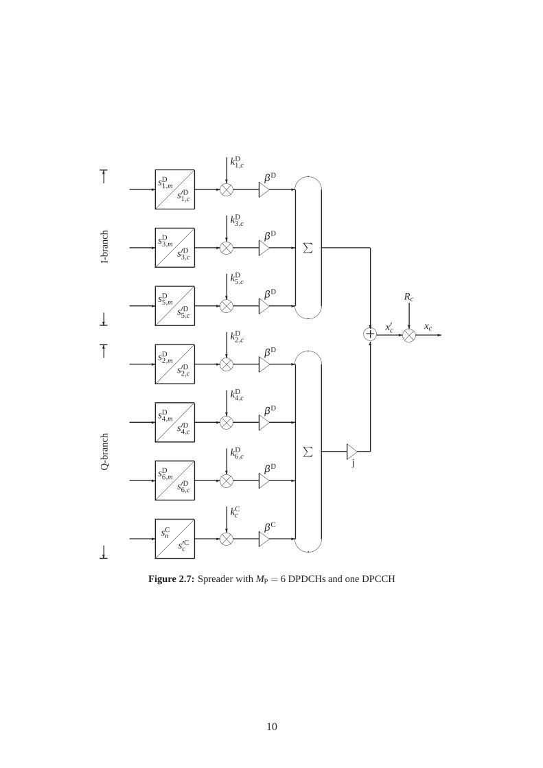
Figure 2.7: Spreader withMP = 6 DPDCHs and one DPCCH

10

wherekx,c ∈

kDµ,c, kC

c

andx = i, j. In the case of spreading factors greater than 4,kx,c isbuilt up by repeating the first four chips periodically. [5] allows the four channelization codes(1 1 1 1), (1 1−1−1), (1−1 1−1) and (1−1−1 1). The first one is reserved for theDPCCH. It must not be used in the I-branch because otherwise no definite channel estimationis possible at the receiver. The other codes may be applied inboth I- and Q-branch. TwoDPDCHs using the same code can be separated due to the factor jin Figure 2.7. Thus,MP = 6 is the maximal possible number of DPDCHs.

We define the DPCCH-to-DPDCH-power ratio

γ = 10· lg DPCCH powerDPDCH power

. (2.6)

According to a certain power ratioγ given by higher layers, the gain factorsβ D andβ C inFigure 2.7 can be derived.

β D =

√

√

√

√

1

MP

(

1+10(γ/10)) (2.7)

β C =

√

√

√

√

10(γ/10)

1+10(γ/10)(2.8)

From Figure 2.7 we obtain

x′c = β D2IP−1∑

i=1

s′Di,c kDi,c + j

(

β Cs′Cc kCc + β D

2QP∑

q=2

s′Dq,c kDq,c

)

, (2.9)

wherei ∈ 1,3,5, q ∈ 2,4,6 and IP+ QP = MP. In general,IP ≤ 3 andQP ≤ IP. x′c ismultiplied by a complex scrambling codeRc enabling the separation of signal contributionsfrom different propagation paths and different terminals at the receiver. Scrambling is appliedeither with long codes or with short codes [5]. Long codes areperiodic with 38400 chips(one frame), whereas the period of the short codes is 256 chips (one DPCCH bit). The latterare used to reduce the computational load if sophisticated multi-user detectors or interferencecancellation receivers are applied [11]. For each type 224 codes are available. They consistof the elements

±1± j

. Scrambling codes are aligned with radio frames, i.e. the first chipof the code appears at the beginning of a frame. For this work only long codes were used.

Finally, the output from the module spreader in Figure 2.3 isgiven as

xc = Rcx′c = Rcβ D

2IP−1∑

i=1

s′Di,c kDi,c + jRc

(

β Cs′Cc kCc + β D

2QP∑

q=2

s′Dq,c kDq,c

)

. (2.10)

11

Figures 2.8 and 2.9 show the constellation diagrams ofx′c andxc, respectively. To simplifymatters, only one DPDCH is multiplexed with the DPCCH (MP = 1). Both the cases (a)γ = 0dB and (b)γ = −3dB are illustrated. The DPCCH-to-DPDCH-power ratioγ = 0dBleads according to (2.7) and (2.8) to the gain factorsβ D = β C = 1/

√2. In this case, we

find the quadrature phase shift keying (QPSK) constellationdiagram ofx′c in Figure 2.8a.Unequal gain factors yield the stretched constellation diagram in Figure 2.8b. However, the

signal points still have the same amplitude. Scrambling causes phase shiftsφc ∈

±π4 ,±3π

4

to each chip. This results in the case of equal gain factors inthe constellation diagram ofxc in Figure 2.9a. It still is a QPSK, rotated byπ

4 . If unequal gain factors are used, we findeight possible signal points in Figure 2.9b with equal powerdistribution between real partand imaginary part.

Due to the special design of the channelization codeskx,c and the scrambling codeRc, thenumber of transitions of the signal through zero is reduced,thus resulting in an improvementof the peak-to-average-power ratio (crest factor). This modulation scheme is called hybridphase shift keying (HPSK) [12]. Naturally, the number of signal points increases if morethan one DPDCH is transmitted.

We turn to Figure 2.3 again. The output from the spreaderxc is multiplied by a gain factorATPC controlling the transmit power of the mobile terminal. Maximal and minimal outputpower depend on the used frequency band and the power class [9]. Transmit power control(TPC) is applied in order to cope with fluctuating receive power at the base station caused byfading. Moreover, multi-user interference (MUI) can be mitigated if the receive powers fromall terminals range at the same level. Two different power control modes can be applied.Open loop power control acts on the receive power of the downlink signal. As this methodworks not very accurately, open loop power control is only used during the initialization ofa transmission. Closed loop power control, in [9, 13] denoted as inner loop power control,adaptsATPC according to theNTPC TPC command bits received via downlink DPCCH. In thefollowing, we assume a transmission system with deactivated power control andATPC= 1.

The pulse shaperG(ω) in Figure 2.3 is a root-raised cosine with roll-off factorα = 0.22 [9].Its impulse responseg(t) is

g(t) =

sin

(

π tTc

(1−α)

)

+4α tTc

cos

(

π tTc

(1+α)

)

π tTc

(

1−(

4α tTc

)2) . (2.11)

g(t) and its amplitude density spectrumG(

f)

are shown in Figure 2.10. The bandwidthamounts approximately tofB = 5MHz.

Hence, the signalx(t) in Figure 2.3 is

x(t) = ATPC

∞∑

c=−∞xcg(t −cTc) , (2.12)

12

(a)

-

6

ℜ

x′c

ℑ

x′c

− 1√2

1√2

− 1√2

1√2

(b)

-

6

ℜ

x′c

ℑ

x′c

−√

23

√

23

− 1√3

1√3

Figure 2.8: Constellation diagram of the chipsx′c consisting of one DPDCH andone DPCCH with power ratios (a)γ = 0dB and (b)γ = −3dB

(a)

-

6

ℜxc

ℑxc

−√

2√

2

−√

2

√2

(b)

-

6

ℜxc

ℑxc

−√

2√

2

−√

2

√2

Figure 2.9: Constellation diagram of the scrambled chipsxc consisting of oneDPDCH and one DPCCH with power ratios (a)γ = 0dB and (b)γ = −3dB

13

−6 −4 −2 0 2 4 6t/Tc

−0.2

0

0.2

0.4

0.6

0.8

1g(t

)/g

(0)

(a)

−4 −2 0 2 4f [MHz]

−100

−80

−60

−40

−20

0

∣ ∣ ∣(G(

f)/G

(0)∣ ∣ ∣

[dB

]

(b)

Figure 2.10: (a) Pulse shaperg(t) in the time domain and (b) its amplitudedensity spectrumG

(

f)

and the transmit signalu(t) after modulation is finally found as

u(t) =√

2ℜ

x(t)e jω0t

, (2.13)

where f0 = ω0/2π is the carrier frequency of the signal. For uplink, three frequency bandsare available: Operating band I (1920−1980MHz), operating band II (1850−1910MHz)and operating band III (1710−1785MHz) [9]. These bands are segmented into channels of5MHz bandwidth. Uplink and downlink frequencies are separated at least by 80MHz. Forcomputer simulation the carrier frequency was set tof0 = 2GHz.

A simulation model of the transmission system, based on discrete-time signal processing inthe baseband, has to satisfy the sampling theorem, i.e. the oversampling frequencyfOS hasto be higher than the signal bandwidthfB. This means for the oversampling clockTOS

TOS =1

fOS≤ 1

fB≈ 200ns. (2.14)

Thus, the integer oversampling factorMOS = Tc/TOS has to be equal to or greater than 2. Inorder to adjust the radio channel delays in an adequate grid,MOS = 4 was chosen for thiswork, i.e.TOS≈ 65ns.

2.4 The mobile radio channel

Additive white Gaussian noise (AWGN) solely is not sufficient to model the mobile radiochannel. The transmitted signal propagates over multiple paths to the receiver as a con-sequence of reflexion, diffraction and scattering. Figure 2.11 illustrates such a channel.Without considering attenuation, each pathr is described by a delayτr (t) and a Doppler

14

R

τ1(t)

, fD1(t)

zτr (t),

fDr(t)

7

τR (t), fDR (t)

u(t)

y(t)

vq

Figure 2.11: Multipath propagation

frequencyfDr (t). Generally, both parameters are time-variant. To simplifymatters, we as-sume in the following constant delaysτr and Doppler frequenciesfDr . The superposition ofthese components leads to random fluctuations of the received signal power, which is alsocalled multipath fading.

Fading effects can be classified in large scale and small scale fading. The first one representschanges of the average received signal power during motion over large distances relative tothe carrier wavelengthλ . It is affected e.g. by hills or high buildings. Transmit power controlcopes with large scale fading. In the work at hand we neglect large scale fading effects.

Small scale fading is characterized by dramatic variationsof the received signal amplitudeand phase as a result of small changes of the location or of theobservation time. If no lineof sight (LOS) component is present, the received signal envelopeε is statistically describedby the Rayleigh probability density function

pε (ε) =

εσ2 e−

ε2

2σ2 ε ≥ 0

0 else, (2.15)

whereσ2 is the mean received signal power.

We have to distinguish two effects that contribute to small scale fading:

15

- Time dispersion of the received signal due to different delaysτr of the pathsr. Thecommunication system under consideration operates with a rake receiver that sepa-rates signal components with a relative delay of at least onechip intervalTc. In thefollowing, we will describe the channel with respect to one single branchl of the rakereceiver, also referred to as finger. It is assumed that all paths contributing to this fingerhave the delayτl .1As inter-chip interference is not present, the fading is frequency flat,e.g. [14].

- Time variance of the channel because of relative motion between transmitter and re-ceiver or due to movement of the scattering objects. This effect leads to an individualDoppler shift for each path, described byfDl ,r , and an overall finger signal dispersionin the frequency domain. The additional indexl assigns the path to one definite finger.

The normalized time-variant equivalent lowpass impulse responsehl (τ, t) with respect tofinger l is then defined as [15]

hl (τ, t) = δ (τ − τl ) ·hl (t) = δ (τ − τl ) · limR→∞

1√R

R∑

r=1

e jΦl ,r+j2π fDl ,rt . (2.16)

τ indicates the signal delay time, andt is the observation time, e.g. [14]. The functionhl (t) isin the following calledfading sequence. It represents the time varying nature of the channel.We assume wide-sense stationary uncorrelated scattering (WSSUS) [15], which means thatthe autocorrelation function ofhl (τ, t) is invariant with respect tot and that the componentsin hl (t) are uncorrelated.Φl ,r is a random phase offset equally distributed within[0,2π).The Doppler frequency

fDl ,r =f0vc

·cos(

αl ,r

)

(2.17)

depends on the angle of arrivalαl ,r at the receiver with respect to the direction of movementwith velocity v. c is the speed of light.fD can be seen as random process with the proba-bility density functionpfD

(

fD)

. In the following, we assume the special case of isotropicscattering described by the Jakes distribution [16]

pfD

(

fD)

=

1

π fD,max

√

1−(

fD/ fD,max)2

∣

∣ fD∣

∣< fD,max

0 else

. (2.18)

1For the derivation of the time-variant equivalent lowpass impulse responseh(τ,t), the finger indexl isused instead of a multipath tap indexz to simplify matters (see Appendix B). Generally, the maximal numberof fingersL is the product of the number of receive antennasA and the number of multipath tapsZ, thusmax(L) = A ·Z.

16

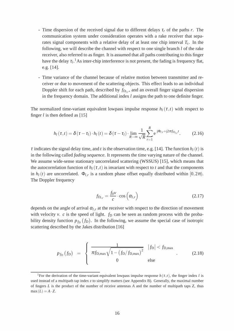
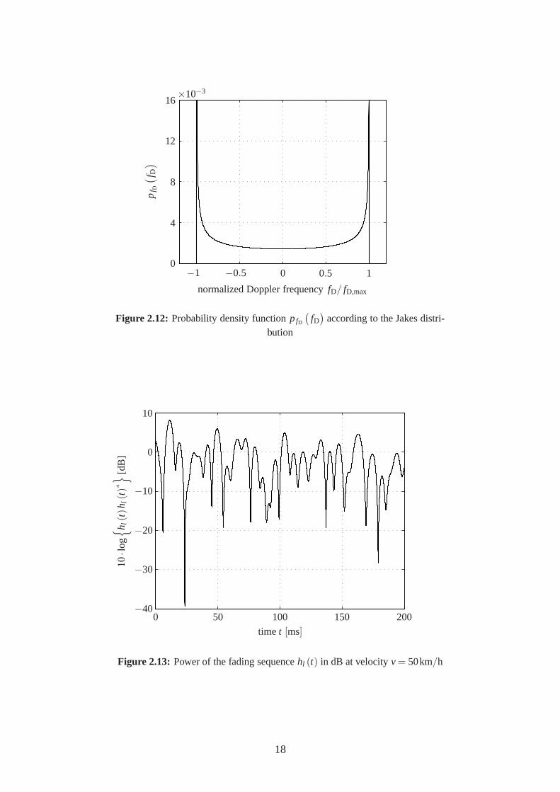
fD,max is the maximal possible Doppler frequency. Figure 2.12 shows the probability densityfunction pfD

(

fD)

that can also be interpreted as the Doppler power density spectrum ofhl (t). Figure 2.13 illustrates an example for the powerhl (t)hl (t)

∗ of a fading sequenceunder consideration of the given assumptions.

The overall equivalent lowpass impulse responseh(τ, t) is given as the superposition of theL fingers that are detected by the rake receiver

h(τ, t) =1

√

∑Ll=1dl

L∑

l=1

√

dl hl (τ, t) =1

√

∑Ll=1dl

L∑

l=1

√

dl δ (τ − τl ) hl (t) , (2.19)

wheredl is a mean power attenuation factor of the fingerl . Generally, the contributions withsmall delayτl exhibit a higher mean received signal power than those with more delay. Theparametersτl anddl of the channel model used for computer simulation are definedin [17]and presented in Appendix B asτz anddz, wherez indicates the multipath tap.

Moreover, the channel model includes AWGN. The long-term signal-to-noise ratio (SNR)is defined asEb/N0. Eb is the average received signal energy per information bit and perantenna from all fingers.N0 represents the one-sided noise power spectral density.

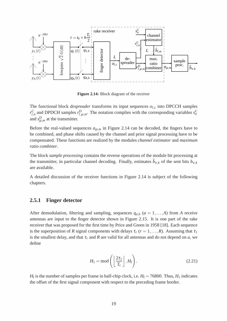
2.5 Physical layer receiver

One possible design of the receiver is illustrated in Figure2.14. It operates withA uncor-related space diversity receive antennas. The radio frequency signal received by antennaa(a = 1, . . . ,A) is denoted asya(t). After demodulation and filtering with the lowpassg(t)from (2.11) we get the baseband signal

qa(t) =√

2(

ya(t)e−jω0t)

⋆g(t) . (2.20)

The amplification factor√

2 is necessary thatqa(t) exhibits the same signal power asx(t)from Figure 2.3 if the channel is ideal.

Samplesqa,h are input to the modulefinger detector. Review, as finger we define a setof unresolvable signal components with almost the same delay. h is discrete-time in half-chip clock. Oversampling by the factor 2 is necessary to meetthe sampling theorem. Ahigher oversampling factor would refine the grid for finger detection. However, complexityincreases without significant performance gain. The finger detector provides one output se-quenceol ,c per fingerl (l = 1, . . . ,L), wherec is discrete-time in chip clock. Finger detectionand separation implies the inverse function of scrambling.

17

−1 −0.5 0 0.5 1

normalized Doppler frequencyfD/ fD,max

0

4

8

12

16×10−3

pf D

(

f D)

Figure 2.12: Probability density functionpfD

(

fD)

according to the Jakes distri-bution

0 50 100 150 200

time t [ms]

−40

−30

−20

−10

0

10

10·lo

g

h l(t

)hl(t

)∗

[dB

]

Figure 2.13: Power of the fading sequencehl (t) in dB at velocityv = 50km/h

18

- -?

y1(t)

e−jω0t···

- -?

yA (t)

e−jω0tlo

wpa

ss√

2G

(ω) -

-

q1 (t)

qA (t)

t = t0 +hTc

2

···

q1,h

qA,h

rake receiver

finge

rde

tect

or

-L

ol ,c

de-spreader

L

-rCl ,n

-rDl ,µ ,m

max.ratio

combiner-

aµ ,m

channelestimator

?hl ,m

-sCn

sampleproc.

-

bν ,k

Figure 2.14: Block diagram of the receiver

The functional blockdespreadertransforms its input sequencesol ,c into DPCCH samplesrCl ,n and DPDCH samplesrD

l ,µ,m. The notation complies with the corresponding variablessCn

andsDµ,m at the transmitter.

Before the real-valued sequencesaµ,m in Figure 2.14 can be decoded, the fingers have tobe combined, and phase shifts caused by the channel and priorsignal processing have to becompensated. These functions are realized by the moduleschannel estimatorandmaximumratio combiner.

The blocksample processingcontains the reverse operations of the module bit processing atthe transmitter, in particular channel decoding. Finally,estimatesbν,k of the sent bitsbν,k

are available.

A detailed discussion of the receiver functions in Figure 2.14 is subject of the followingchapters.

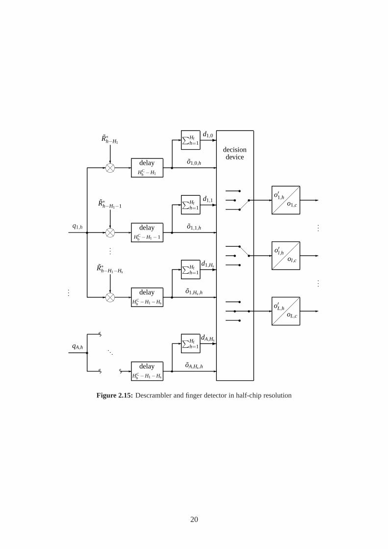
2.5.1 Finger detector

After demodulation, filtering and sampling, sequencesqa,h (a = 1, . . . ,A) from A receiveantennas are input to the finger detector shown in Figure 2.15. It is one part of the rakereceiver that was proposed for the first time by Price and Green in 1958 [18]. Each sequenceis the superposition ofR signal components with delaysτr (r = 1, . . . ,R). Assuming thatτ1

is the smallest delay, and thatτr andR are valid for all antennas and do not depend ona, wedefine

H1 = mod

(

⌊

2τ1

Tc

⌋

,Hf

)

. (2.21)

Hf is the number of samples per frame in half-chip clock, i.e.Hf = 76800. Thus,H1 indicatesthe offset of the first signal component with respect to the preceding frame border.

19

q1,h

-

-

-···

qA,h · · ·

?

R∗h−H1

-

-

?

R∗h−H1−1

-

-

···

?

R∗h−H1−Hs

-

-

-

-

delay

delay

delay

delay

∑Hfh=1

∑Hfh=1

∑Hfh=1

∑Hfh=1

-o1,0,h

-o1,1,h

-o1,Hs,h

-oA,Hs,h

-d1,0

-d1,1

-d1,Hs

-dA,Hs

decisiondevice

-

-

-

o′1,ho1,c

o′l ,hol ,c

o′L,hoL,c

-

···

-

···

-

HCb −H1

HCb −H1−1

HCb −H1−Hs

HCb −H1−Hs

Figure 2.15: Descrambler and finger detector in half-chip resolution

20

Firstly, each input signalqa,h is split up in Hs+ 1 branches.Hs determines the maximalpossible delayτmax of signal components that can be detected.

τmax = τ1+Hs ·Tc

2(2.22)

In each branchξ (ξ = 0, . . . ,Hs) the samplesqa,h are multiplied by the delayed conjugate

complex scrambling sequenceR∗h−H1−ξ , whereRh = Rc with c =

⌈

h2

⌉

. We considerRh aspseudo noise sequence with periodHf. This operation is called descrambling. The resultis delayed byHC

b −H1− ξ in order to synchronize all branches to the subsequent DPCCHbit interval border, which simplifies the following signal processing.HC

b is the number ofsamples within the smallest possible integer number of DPCCH bits, i.e.

HCb = 512·

⌈

H1+Hs

512

⌉

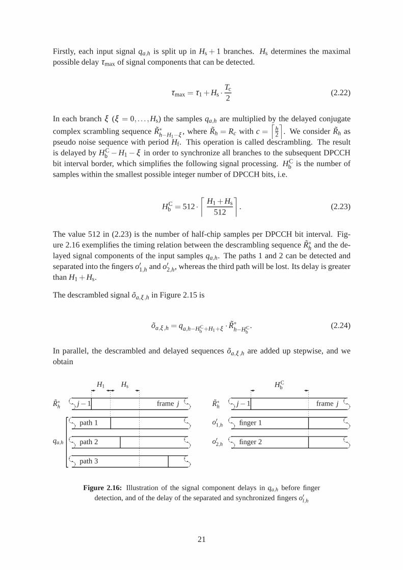
. (2.23)

The value 512 in (2.23) is the number of half-chip samples perDPCCH bit interval. Fig-ure 2.16 exemplifies the timing relation between the descrambling sequenceR∗

h and the de-layed signal components of the input samplesqa,h. The paths 1 and 2 can be detected andseparated into the fingerso′1,h ando′2,h, whereas the third path will be lost. Its delay is greaterthanH1+Hs.

The descrambled signal ˜oa,ξ ,h in Figure 2.15 is

oa,ξ ,h = qa,h−HCb +H1+ξ · R∗

h−HCb. (2.24)

In parallel, the descrambled and delayed sequences ˜oa,ξ ,h are added up stepwise, and weobtain

R∗h j −1 frame j

path 1

path 2

path 3

qa,h

- -H1 Hs

R∗h j −1 frame j

finger 1o′1,h

finger 2o′2,h

-HCb

Figure 2.16: Illustration of the signal component delays inqa,h before fingerdetection, and of the delay of the separated and synchronized fingerso′l ,h

21

da,ξ =150∑

m=1

∣

∣

∣

∣

∣

∣

∣

512m∑

h=512(m−1)+1

oa,ξ ,h

∣

∣

∣

∣

∣

∣

∣

=150∑

m=1

∣

∣

∣

∣

∣

∣

∣

512m∑

h=512(m−1)+1

qa,h−HCb +H1+ξ · R∗

h−HCb

∣

∣

∣

∣

∣

∣

∣

. (2.25)

The valuesqa,h include one component originating from the DPCCH that does not changeduring one DPCCH bit interval, i.e. 512 samples, because thechip-invariant spreading codekC

c = (1 1 1 1) was used. The finger detector takes all valuesda,ξ to decide whether a signalcomponent with delayτr ≈ τ1 + ξ · Tc

2 is present inqa,h. In this case,da,ξ will exhibit asignificant higher value due to maximal correlation betweenR∗

h−H1−ξ andqa,h compared toa non-existing path.

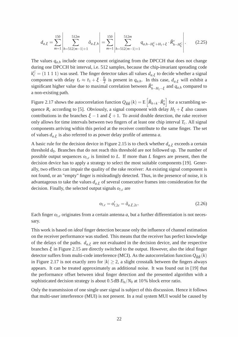
Figure 2.17 shows the autocorrelation functionQRR(k) = E[

Rh+k · R∗h

]

for a scrambling se-

quenceRc according to [5]. Obviously, a signal component with delayH1 + ξ also causescontributions in the branchesξ −1 andξ +1. To avoid double detection, the rake receiveronly allows for time intervals between two fingers of at leastone chip intervalTc. All signalcomponents arriving within this period at the receiver contribute to the same finger. The setof valuesda,ξ is also referred to as power delay profile of antennaa.

A basic rule for the decision device in Figure 2.15 is to checkwhetherda,ξ exceeds a certainthresholdd0. Branches that do not reach this threshold are not followed up. The number ofpossible output sequencesol ,c is limited to L. If more thanL fingers are present, then thedecision device has to apply a strategy to select the most suitable components [19]. Gener-ally, two effects can impair the quality of the rake receiver: An existing signal component isnot found, or an "empty" finger is misleadingly detected. Thus, in the presence of noise, it isadvantageous to take the valuesda,ξ of several consecutive frames into consideration for thedecision. Finally, the selected output signalsol ,c are

ol ,c = o′l ,2c = oa,ξ ,2c. (2.26)

Each fingerol ,c originates from a certain antennaa, but a further differentiation is not neces-sary.

This work is based onidealfinger detection because only the influence of channel estimationon the receiver performance was studied. This means that thereceiver has perfect knowledgeof the delays of the paths.da,ξ are not evaluated in the decision device, and the respectivebranchesξ in Figure 2.15 are directly switched to the output. However,also the ideal fingerdetector suffers from multi-code interference (MCI). As the autocorrelation functionQRR(k)in Figure 2.17 is not exactly zero for|k| ≥ 2, a slight crosstalk between the fingers alwaysappears. It can be treated approximately as additional noise. It was found out in [19] thatthe performance offset between ideal finger detection and the presented algorithm with asophisticated decision strategy is about 0.5dBEb/N0 at 10% block error ratio.

Only the transmission of one single user signal is subject ofthis discussion. Hence it followsthat multi-user interference (MUI) is not present. In a realsystem MUI would be caused by

22

−12 −8 −4 0 4 8 12k

0.0

0.5

1.0

1.5

2.0

auto

corr

elat

ion

func

tionℜ

QR

R(k

)

Figure 2.17: Real part of the autocorrelation functionQRR(k) of the scramblingsequenceRh

the cross correlation between two scrambling sequencesR1,h of user 1 andR2,h of user 2.MUI can lead to a severe performance degradation for a large number of users.

Several ideas how to combat MCI and MUI were discussed in the literature. One importantexample is successive interference cancellation. It can beseen as recursive finger detectionand channel estimation. The strongest paths are identified one after the other, and theircontributions to the received signal are suppressed beforegoing to the next loop iteration.The disadvantage of this algorithm is the high complexity. [20] presents a solution withreduced complexity for the 3G framework.

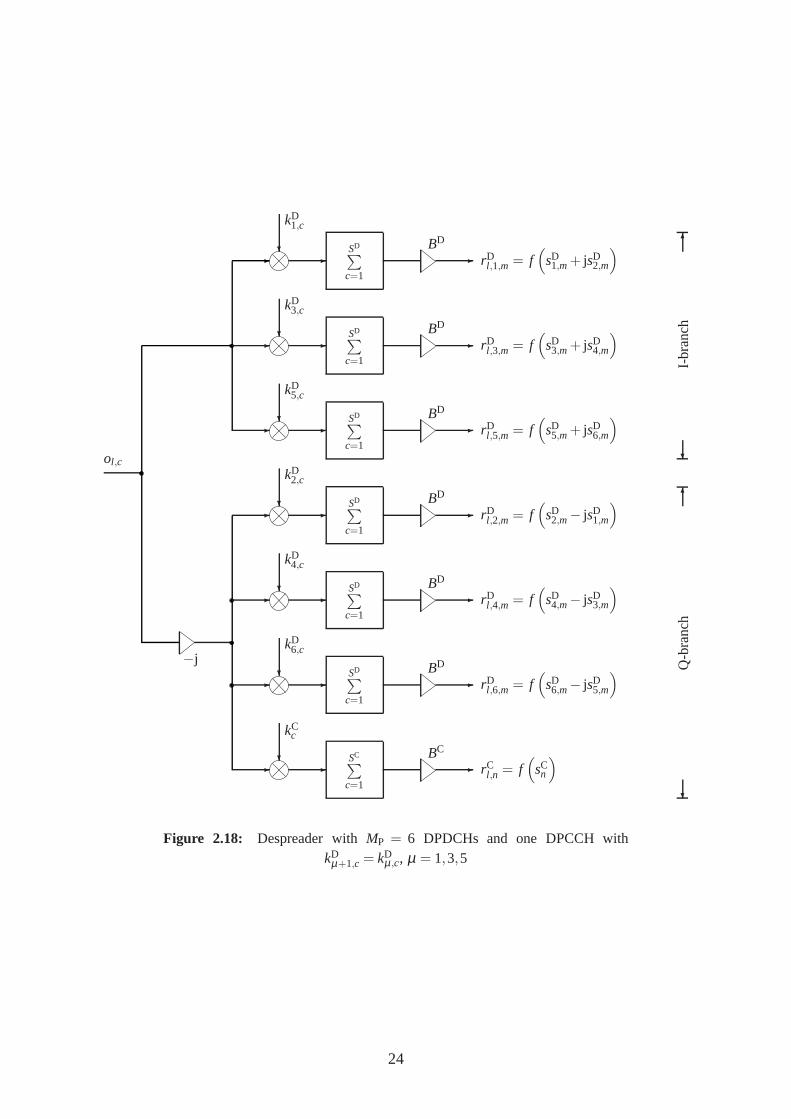
2.5.2 Despreader

After the signal components in the sequencesqa,h have been detected and separated intofingersol ,c, we now want to demultiplex the physical channels and to return to a signalrepresentation in bit clock. The despreader in Figure 2.18 executes the reverse function ofthe spreader in Figure 2.7. Each fingerol ,c is split up into an I-branch and a Q-branch. Thephase of the latter was shifted byπ/2 at the transmitter. Hence it follows that we have tomultiply firstly by−j.

Afterwards, the signals in both branches are multiplied by the associated spreading codeskD

µ,c andkCc . For the six DPDCHs in Figure 2.18 only three different codesare available, and

we assumekD1,c = kD

2,c, kD3,c = kD

4,c andkD5,c = kD

6,c. Due to this twofold assignment a uniquerecovery of the DPDCHs is not possible by despreading solely. Each sequencerD

l ,µ,m includes

23

ol ,c

−j

-?

kD1,c

-SD∑

c=1

BD

- rDl ,1,m = f

(

sD1,m+ jsD

2,m

)

-?

kD3,c

-SD∑

c=1

BD

- rDl ,3,m = f

(

sD3,m+ jsD

4,m

)

-?

kD5,c

-SD∑

c=1

BD

- rDl ,5,m = f

(

sD5,m+ jsD

6,m

)

-?

kD2,c

-SD∑

c=1

BD

- rDl ,2,m = f

(

sD2,m− jsD

1,m

)

-?

kD4,c

-SD∑

c=1

BD

- rDl ,4,m = f

(

sD4,m− jsD

3,m

)

-?

kD6,c

-SD∑

c=1

BD

- rDl ,6,m = f

(

sD6,m− jsD

5,m

)

-?

kCc

-SC∑

c=1

BC

- rCl ,n = f

(

sCn

)

6

?

I-br

anch

6

?

Q-b

ranc

h

Figure 2.18: Despreader withMP = 6 DPDCHs and one DPCCH withkD

µ+1,c = kDµ ,c, µ = 1,3,5

24

a component originating from another DPDCH whose phase is shifted by ±π/2. Lateron, we will see that this effect will not necessarily interfere with the receiver performance.However, one has to be aware of this fact.

SamplesrDl ,µ,m can be determined by summation overSD chips and scaling with a factorBD.

The summation in the DPCCH branch spansSC chips, and a different scaling factorBC isapplied to getrC

l ,n. We finally yield

rDl ,µ,m =

BDSD∑

c=1ol ,c kD

µ,c µ = 1,3,5

−j BDSD∑

c=1ol ,c kD

µ,c µ = 2,4,6

(2.27)

and

rCl ,n = −j BC

SC∑

c=1

ol ,c kCc . (2.28)

The factorsBD andBC in Figure 2.18 scale the output such thatrDl ,µ,m = ±1 andrC

l ,n = ±1under the assumption of an ideal channel and unique recoveryof the DPDCHs. We obtain

BD =1

2 ·SD ·β D (2.29)

and

BC =1

2 ·SC ·β C . (2.30)

The factor 2 in (2.29) and (2.30) comes from the amplificationdue to spreading and de-spreading.

In spread spectrum systems the ratio between the signal-to-noise ratios after and before de-spreading is called processing gain. It can be shown easily that the processing gains of theDPDCHs and of the DPCCH are equal to the spreading factorsSD andSC = 256, respec-tively [21].

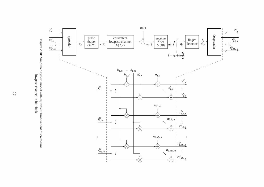
2.5.3 Simplified system model

After a detailed discussion of the transmission system up tothe despreader, the simplifiedsystem model according to Figures 2.19 and 2.20 will be considered in the following. Itallows for a direct relation between the input signalssD

µ,m andsCn to the spreader and the

25

-x(t)

?

e jω0t

- √2 ℜ -

u(t)bandpass channel

b(τ , t)-

?

n(t)

-y(t)

?

e−jω0t

-√2 r id (t) -

w(t)

-x(t)

equivalentlowpass channel

h(τ , t)-

?

n(t)

-w(t)

Figure 2.19: Time-variant equivalent lowpass channel

despreader outputsrDl ,µ,m andrC

l ,n. Hence it follows that channel estimation and maximumratio combining can be presented more intelligibly.

Firstly, we turn to the equivalent lowpass channel model in Figure 2.19. The upper branchconsists of transmitter elements described previously.b(τ, t) is the time-variant bandpassimpulse response of the mobile radio channel, and ˜n(t) represents stationary AWGN withzero mean that exhibits a certainEb/N0. The demodulator is part of the known receiver blockdiagram. The antenna indexa is left out to simplify matters. Moreover, the model requiresan ideal lowpass filterr id (t) that eliminates signal components around 2ω0, i.e.

r id (t) −• Rid(

f)

=

1∣

∣ f∣

∣≤ fB/20 else

. (2.31)

h(τ, t) in the lower branch is the already derived time-variant equivalent lowpass impulseresponse of the channel according to (2.19).n(t) is filtered baseband noise. The ideallowpassr id (t) has no impact onEb/N0. The equivalence of both branches is shown e.g. in[22]. w(t) is the response of the time-variant mobile radio channel to the baseband transmitsignalx(t). According to [23], it is

w(t) =

−∞∫

−∞

h(τ, t)x(t − τ)dτ + n(t) . (2.32)

Now, we turn to the equivalent discrete-time model in Figure2.20. We define

rDl ,µ,m = hl ,m

(

sDµ,m± jsD

q,m

)

+ nl ,µ,m (2.33)

and

26

-sCn

-sD1,m

···

-sDMP,m

spreader

-xc

pulseshaperG(ω)

-x(t)

equivalentlowpass channel

h(τ , t)-

?

n(t)

-w(t)

receivefilterG(ω) q(t)

t = t0 +hTc

2

-qh

fingerdetector

-Lol ,c

despreader

-rCl ,n

-rDl ,1,m

···

-rDl ,MP,m

L

sCn ··

· ···

- - -rC1,n

- - -rCL,n

sD1,m

··· ···

- - -rD1,1,m

- - -rDL,1,m

···

···

sDMP,m

··· ···

- - -rD1,MP,m

- - -rDL,MP,m

h1,m · · ·

?

h′1,n· · ·

?

?

hL,m

?

h′L,n

?

?

n1,1,m

?

n′1,n

?

n1,MP,m

?

n′L,n

?

nL,1,m

?

nL,MP,m

?

· · ·· · ·

· · ·

Figure

2.20:Sim

plifiedsystem

modelw

ithequivalenttim

e-variantdiscrete-tim

elow

passchannelin

bitclock

27

rCl ,n = h′l ,n sC

n +n′l ,n, (2.34)

whereµ = 1, . . . ,MP andq = µ ±1 according to the notation used in Figure 2.18. The com-ponentsD

q,m in (2.33) is only present if the same spreading codekDµ,c was applied to both

DPDCHsµ andq. It is left out in Figure 2.20 to simplify matters.hl ,m andh′l ,n are complex-valued samples of the fading sequenceshl (t), in the following referred to aschannel coef-ficients. Without loss of generality, the same coefficientshl ,m are applied to all DPDCHsµ. Moreover, we defineh′l ,n = hl ,m with m= n ·SC/SD. nl ,µ,m andn′l ,n are filtered and de-spread noise originating fromn(t). Generally, they also include the impact of multi-codeand multi-user interference as well as impairments due to finger detection errors. The latterare excluded in the work at hand because we study a receiver with ideal finger detection ina single-user transmission system. Computer simulation has shown thatnl ,µ,m andn′l ,n canbe assumed as realizations of complex random processes, where both real- and imaginarypart exhibit Gaussian distribution with zero mean. The variances are denoted asσ2

D for theDPDCHs and asσ2

C for the DPCCH, respectively.

2.5.4 Channel estimator and maximum ratio combiner

Task of the module channel estimator in Figure 2.14 is to provide estimateshl ,m of the chan-nel coefficientshl ,m. In Chapters 3 - 5, various methods will be investigated and comparedfor this purpose. Because of noise, the channel estimator will cause an estimation errorel ,m.It follows thathl ,m can be written as

hl ,m = hl ,m+el ,m. (2.35)

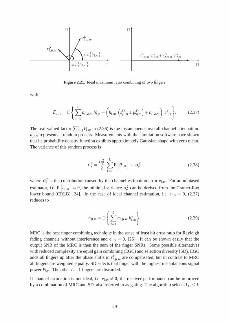
The estimateshl ,m are input to the functional block maximum ratio combiner (MRC) thathas to combine the finger signalsrD

l ,µ,m in the best possible way. From (2.33) follows that thecomplex channel coefficientshl ,m cause phase shifts. This is exemplified forL = 2 fingers inFigure 2.21. Multiplication byh∗l ,m rotates the desired component originating from DPDCHµ onto the real axis, whereas the undesired contribution fromDPDCH q is located on theimaginary axis. This operation also leads to a weighting according to the instantaneouspowerPl ,m = hl ,m h∗l ,m. The combined signalaµ,m is defined as

aµ,m = ℜ

L∑

l=1

rDl ,µ,m h∗l ,m

(2.33,2.35)= ℜ

L∑

l=1

(

hl ,m

(

sDµ,m± jsD

q,m

)

+nl ,µ,m

)

·(

h∗l ,m+e∗l ,m)

= sDµ,m

L∑

l=1

Pl ,m + nµ,m (2.36)

28

-

ℜ

6ℑ

-

ℜ

6ℑ

IY

rD1,µ ,m

arc

h1,m

rD2,µ ,m

arc

h2,m

- -rD1,µ ,m ·h∗1,m+ rD

2,µ ,m ·h∗2,m

Figure 2.21: Ideal maximum ratio combining of two fingers

with

nµ,m = ℜ

L∑

l=1

nl ,µ,m h∗l ,m+

(

hl ,m

(

sDµ,m± jsD

q,m

)

+nl ,µ,m

)

e∗l ,m

. (2.37)

The real-valued factor∑L

l=1Pl ,m in (2.36) is the instantaneous overall channel attenuation.nµ,m represents a random process. Measurements with the simulation software have shownthat its probability density function exhibits approximately Gaussian shape with zero mean.The variance of this random process is

σ2a =

σ2D

2

L∑

l=1

E[

Pl ,m

]

+ σ2e , (2.38)

whereσ2e is the contribution caused by the channel estimation errorel ,m. For an unbiased

estimator, i.e. E[

el ,m

]

= 0, the minimal varianceσ2e can be derived from the Cramer-Rao

lower bound (CRLB) [24]. In the case of ideal channel estimation, i.e. el ,m = 0, (2.37)reduces to

nµ,m = ℜ

L∑

l=1

nl ,µ,m h∗l ,m

. (2.39)

MRC is the best finger combining technique in the sense of least bit error ratio for Rayleighfading channels without interference andel ,m = 0. [25]. It can be shown easily that theoutput SNR of the MRC is then the sum of the finger SNRs. Some possible alternativeswith reduced complexity are equal gain combining (EGC) and selection diversity (SD). EGCadds all fingers up after the phase shifts inrD

l ,µ,m are compensated, but in contrast to MRCall fingers are weighted equally. SD selects that finger with the highest instantaneous signalpowerPl ,m. The otherL−1 fingers are discarded.

If channel estimation is not ideal, i.e.el ,m 6= 0, the receiver performance can be improvedby a combination of MRC and SD, also referred to as gating. Thealgorithm selectsLG ≤ L

29

available rake fingers such that the output SNR of the combiner is maximized [26]. However,the additional complexity is significant. The idea was not followed up in the work at hand.

2.5.5 Sample processing

The module sample processing in Figure 2.14 inverts all operations that were applied tothe bitsbν,k at the transmitter by the block bit processing [4]. Some functions, namelydeinterleaving and channel demapping, allow a one-to-one assignment between input andoutput. If puncturing was carried out by the transmitter rate matching algorithm, neutralzeros have to be inserted into the sequence at the receiver.

However, the major task is channel decoding. The added redundancy is thereby utilized tolower the bit error ratio. For convolutionally coded transport channels the Viterbi algorithmis applied, which determines the most probable bit sequences bν,k [27,28].

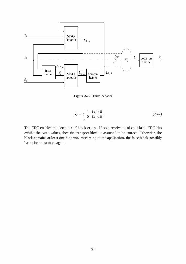
Received turbo coded transport channels are composed of systematic samples ˜xk as wellas parity samples ˜zk and z′k as shown in Figure 2.22. These samples correspond to the re-spective sent bitsxk,zk andz′k. The received termination samplesT are left out to simplifymatters. The decoder consists of two soft-in soft-out (SISO) decoders, e.g. [29], that are

connected through interleavers. They determinea posterioriprobabilities P[

xk = 1 | X]

and

P[

x′k = 1 | X′]

, respectively, whereX is a vector containing all values ˜xk. The L-valuesL12,k

andL′21,k are defined as

L12,k = lnP[

xk = 1 | X]

P[

xk = 0 | X] (2.40)

and

L′21,k = ln

P[

x′k = 1 | X′]

P[

x′k = 0 | X′] . (2.41)

Each SISO decoder updates thea priori knowledge of the other decoder by itsa posterioridecoding result, an interaction similar to a turbo engine. This iterative algorithm was firstlyproposed by Berrou et al. in 1993 [30]. It exhibits error correcting capabilities close tothe limit postulated by Shannon in 1948 [31]. One main parameter is the number of callsIT of each decoder, in this work called turbo iterations. AfterIT turbo iterations, valuesLk = Lchxk +L12,k +L21,k are determined.Lch is called channel L-value and depends on themean SNR of the decoder input samples. The decision device inFigure 2.22 finally providesestimates ˆxk of the sent bitsxk, namely

30

-zk

xk

-

-

-z′k

SISOdecoder L12,k

-inter-leaver

-L′

12,k

-x′k SISO

decoder-

L′21,k deinter-

leaver

L21,k

-

Lch

-

-

-

∑ -Lk decision

device-xk

Figure 2.22: Turbo decoder

xk =

1 Lk ≥ 00 Lk < 0

. (2.42)

The CRC enables the detection of block errors. If both received and calculated CRC bitsexhibit the same values, then the transport block is assumedto be correct. Otherwise, theblock contains at least one bit error. According to the application, the false block possiblyhas to be transmitted again.

31

Chapter 3

Channel estimation without feedback

As already mentioned previously, the channel estimator provides estimateshl ,m of the time-varying channel coefficientshl ,m for each fingerl (l = 1, . . . ,L). In this chapter, at first thefundamental mechanism of channel estimation is described.Afterwards, several pilot aidedalgorithms based on the segmentation of the DPCCH accordingto Figure 2.2 are discussedin detail.

To simplify notation, we will consider only one rake finger and omit indexl in the following.Of course, channel estimation has to be carried out for each finger individually. Moreover,we assume without loss of generality thatMP = 1 DPDCH is transmitted. Therefore, alsothe DPDCH indexµ is left out. The simplified system model (2.33, 2.34) becomes

rDm = hm sD

m+nm (3.1)

and

rCn = h′n sC

n +n′n. (3.2)

In a first step, we assume that all DPCCH bitssCn are pilot bits and known at the receiver. In

the noise-free case,h′n can be determined exactly by multiplying the received samplesrCn by

sCn . As we already know,sC

n ∈ ±1, i.e.

χn = rCn sC

n = h′n sCn sC

n = h′n. (3.3)

In the following, this operation is calledpilot compensation, and we denoteχn as com-pensated pilot samples. In the presence of noise, estimatesh′n of h′n can be determined byaveraging overNA compensated pilot samplesχn. As the noisen′n exhibits zero mean, itsimpact onh′n is reduced because

33

limNA→∞

1NA

n+N′A

∑

ν=n−N′A

n′ν = 0 (3.4)

with NA = 2N′A +1. Thus, we yield

h′n =1

NA

n+N′A

∑

ν=n−N′A

χν =1

NA

n+N′A

∑

ν=n−N′A

h′ν +1

NA

n+N′A

∑

ν=n−N′A

n′ν sCν . (3.5)

Considering (3.4), estimatesh′n become for highNA approximately

h′n =1

NA

n+N′A

∑

ν=n−N′A

χν ≈ 1NA

n+N′A

∑

ν=n−N′A

h′ν . (3.6)

In the special case of a time-invariant channel with the constant coefficienth′n = h′, (3.5)becomes

h′n = h′ +1

NA

n+N′A

∑

ν=n−N′A

n′ν sCν . (3.7)

Aim of the channel estimator is to provide estimateshm of the DPDCH channel coefficientshm. We assume both physical channel signals passing through the same fading sequenceh(t). It follows thathm = h′n with n =

⌈

m/M′⌉. The ratioM′ = SC/SD denotes the numberof DPDCH bits per DPCCH bit interval.

The parameterNA is related to the channel observation timeTobs that we define as

Tobs= NA ·TCb , (3.8)

whereTCb = SC · Tc ≈ 66.7µs is the DPCCH bit interval. Generally, the impact of noise

is reduced more for longerTobs. On the other hand, a too long channel observation timewill degrade the tracking ability of the estimator.h′n is time-variant, and its rate of changeis related to the speed of the mobile terminal. The estimatortherefore has to be adaptedaccording to the instantaneous channel conditions. As a general rule,Tobs has to be set aslong as the time variation ofh′n allows for.

After this brief introduction some sophisticated approaches to determineh′n andhm, respec-tively, are presented and compared in the following chapters.

34

3.1 Weighted multi-slot averaging (WMSA)

3.1.1 The basic principle

The idea of WMSA was firstly published by NTT DoCoMo in 1997 [32]. The derivation re-quires to indicate the current sloti in addition to the bit indicesm= 1, . . . ,M for the DPDCHandn = 1, . . . ,N for the DPCCH. We therefore replace (3.1) and (3.2) by

rDi,m = hi,m sD

i,m+ni,m (3.9)

and

rCi,n = h′i,n sC

i,n+n′i,n. (3.10)

Furthermore, we assume that the DPDCH exhibits a relative delay of four slots comparedto the DPCCH. Hence, samplesrC

i+4,n are input to the channel estimator, whereas the MRC

processes samplesrDi,m and estimateshi,m. The delay of four slots was predefined arbitrarily.

It allows to consider both past slots (i−4, . . . , i−1) and future slots (i +1, . . . , i +4) for chan-nel estimation if we define sloti as present time. It was shown by computer simulation thata smaller delay would unnecessarily limit the noise reduction for slowly changing channelconditions, whereas a processing delay of more than four slots increases complexity withoutsignificant performance gain.

The channel estimation error from (2.35) is now denoted as

ei,m = hi,m−hi,m. (3.11)

A detailed analysis of the WMSA channel estimation error is presented in [33]. Furthermore,we define the channel estimation phase errorϕi,m as

ϕi,m = arc

hi,m

−arc

hi,m

. (3.12)

The WMSA algorithm provides one estimatehWMSAi per sloti, namely

hWMSAi =

1∑i+4

κ=i−4wκ

i+4∑

κ=i−4

wκNP

NP∑

n=1

χκ,n

=1

∑i+4κ=i−4wκ

i+4∑

κ=i−4

wκ χκ . (3.13)

The mean value of the compensated pilot samplesχκ,n of the slotκ is calledinstantaneouschannel estimateχκ . The factorswκ enable to weight the contribution of each slot individ-ually. Naturally, in (3.13) contributions near to the present slotκ = i are weighted stronger

35

than others. The impact of the time-variance ofh′i,n on the estimatehWMSAi is thereby re-

duced. We define the vector

w =[

wi−4 . . .wi . . .wi+4]

(3.14)

as WMSA weighting vector andI as WMSA filter length, which is the number of adjacentelementswκ 6= 0 in the vectorw. Normally, these elements are located in the center ofw,whereas elementswκ = 0 only occur at the left and the right border. The latter are omittedto simplify matters. The reason is that contributions from slots κ near to the present slotiare weighted stronger than others. The elementwi in (3.14), representing the present slot, isstressed with bold font. As an example, the WMSA weighting vector w = [0.3 0.6 1.0 0.5]

considers the slotsκ = i −2, . . . , i +1, and the WMSA filter length isI = 4.

Figure 3.1 clarifies how the estimatehWMSAi results from (3.13). Obviously, only the instan-

taneous channel estimatesχκ have to be stored, but not the compensated pilot samplesχκ,n

themselves. The two-stage calculation reduces complexity. This is one big advantage ofWMSA, particularly with respect to its realization on a digital signal processor. On the otherhand, WMSA considers each slot either complete or not at all,i.e. I is an integer number.For fast changing channel conditions that require a small WMSA window length, this mayturn out to be a disadvantage.

The MRC requires according to (2.36) one channel estimatehi,m per DPDCH bit interval.We definehWMSA

i,m = hWMSAi for m= 1, . . . ,M. As a consequence, WMSA provides for some

samplesm only a rough estimation ofhi,m. This is a serious issue if two DPDCHsµ andqare transmitted with the same spreading codekD

µ,c. The combined signalaµ,m in (2.36) maythen include a considerable contribution from the DPDCHq.

Figure 3.2 illustrates an example for the impact of the WMSA filter lengthI and the signal-to-noise ratioEb/N0 on hWMSA

i . The speed of the mobile terminal is 120km/h. Values

ℜ

hWMSAi

achieved with WMSA weighting vectorsw = [1] andw = [1 1 1 11 1 1 1 1],

i.e. I = 1 andI = 9, are compared with the actual channelℜ

hi,m

.

The left diagram shows the noise-free case. Since only the time variation ofhi,m is degradingthe quality ofhWMSA

i , the WMSA weighting vector with the short filter lengthI = 1, show-ing optimal tracking behavior, provides the better result.In contrast, estimation withI = 9follows the channel coefficientshi,m inadequately.

On the right hand side, we can see that the very bad signal-to-noise ratioEb/N0 = 0dB hasonly little impact on the estimateshWMSA

i achieved with the WMSA filter lengthI = 9. Theshort vector withI = 1 causes a tremendous increase of the channel estimation error ei,m

because the contribution of noise is not suppressed sufficiently.

The presented results lead to the question which WMSA weighting vector will provide thesmallest channel estimation error and the lowest BLER at a given speed of the mobile termi-nal.

36

j

?

? ? ?-

CE input χi+4,1 · · ·

· · ·

χi+4,NP

∑

1NP

shift register

χi−4 · · · χi · · · χi+4

wi−4 · · · wi · · · wi+4

∑

1∑i+4

κ=i−4wκ

hWMSAi

Figure 3.1: Implementation model of the WMSA algorithm

actual channelWMSA with I = 1WMSA with I = 9

0 4 8 12 16time [ms]

−1

−0.5

0

0.5

1

ℜ

ampl

itude

(a)

actual channelWMSA with I = 1WMSA with I = 9

actual channelWMSA with I = 1WMSA with I = 9

0 4 8 12 16time [ms]

−1

−0.5

0

0.5

1

ℜ

ampl

itude

(b)

actual channelWMSA with I = 1WMSA with I = 9

Figure 3.2: WMSA channel estimateshWMSAi with filter lengths I = 1 and

I = 9 in comparison with the actual channelhi,m (a) without noise and (b) withEb/N0 = 0dB

37

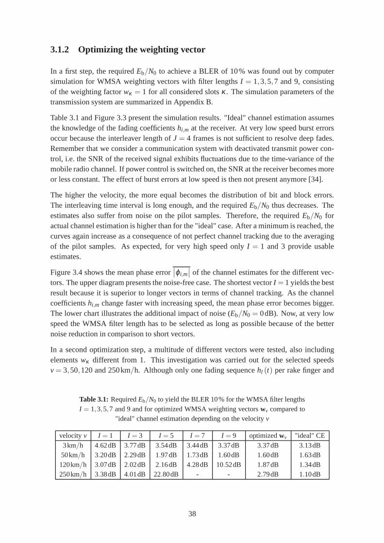
3.1.2 Optimizing the weighting vector

In a first step, the requiredEb/N0 to achieve a BLER of 10% was found out by computersimulation for WMSA weighting vectors with filter lengthsI = 1,3,5,7 and 9, consistingof the weighting factorwκ = 1 for all considered slotsκ . The simulation parameters of thetransmission system are summarized in Appendix B.

Table 3.1 and Figure 3.3 present the simulation results. "Ideal" channel estimation assumesthe knowledge of the fading coefficientshi,m at the receiver. At very low speed burst errorsoccur because the interleaver length ofJ = 4 frames is not sufficient to resolve deep fades.Remember that we consider a communication system with deactivated transmit power con-trol, i.e. the SNR of the received signal exhibits fluctuations due to the time-variance of themobile radio channel. If power control is switched on, the SNR at the receiver becomes moreor less constant. The effect of burst errors at low speed is then not present anymore [34].

The higher the velocity, the more equal becomes the distribution of bit and block errors.The interleaving time interval is long enough, and the requiredEb/N0 thus decreases. Theestimates also suffer from noise on the pilot samples. Therefore, the requiredEb/N0 foractual channel estimation is higher than for the "ideal" case. After a minimum is reached, thecurves again increase as a consequence of not perfect channel tracking due to the averagingof the pilot samples. As expected, for very high speed onlyI = 1 and 3 provide usableestimates.

Figure 3.4 shows the mean phase error∣

∣ϕi,m∣

∣ of the channel estimates for the different vec-tors. The upper diagram presents the noise-free case. The shortest vectorI = 1 yields the bestresult because it is superior to longer vectors in terms of channel tracking. As the channelcoefficientshi,m change faster with increasing speed, the mean phase error becomes bigger.The lower chart illustrates the additional impact of noise (Eb/N0 = 0dB). Now, at very lowspeed the WMSA filter length has to be selected as long as possible because of the betternoise reduction in comparison to short vectors.

In a second optimization step, a multitude of different vectors were tested, also includingelementswκ different from 1. This investigation was carried out for theselected speedsv = 3,50,120 and 250km/h. Although only one fading sequencehl (t) per rake finger and

Table 3.1: RequiredEb/N0 to yield the BLER 10% for the WMSA filter lengthsI = 1,3,5,7 and 9 and for optimized WMSA weighting vectorswv compared to

"ideal" channel estimation depending on the velocityv

velocity v I = 1 I = 3 I = 5 I = 7 I = 9 optimizedwv "ideal" CE

3km/h 4.62dB 3.77dB 3.54dB 3.44dB 3.37dB 3.37dB 3.13dB50km/h 3.20dB 2.29dB 1.97dB 1.73dB 1.60dB 1.60dB 1.63dB120km/h 3.07dB 2.02dB 2.16dB 4.28dB 10.52dB 1.87dB 1.34dB250km/h 3.38dB 4.01dB 22.80dB - - 2.79dB 1.10dB

38

I = 1I = 3I = 5I = 7I = 9optimized w

i

"ideal" CE

0 50 100 150 200 250

velocity v[

km/h]

1

2

3

4

5

Eb/

N0[d

B]

I = 1I = 3I = 5I = 7I = 9optimizedwv

"ideal" CE

Figure 3.3: RequiredEb/N0 to yield the BLER 10% for the WMSA filter lengthsI = 1,3,5,7 and 9 and for optimized WMSA weighting vectorswv compared to

"ideal" channel estimation depending on the velocityv

39

I = 1I = 3I = 5I = 7I = 9optimized w

i

0 50 100 150 200 250velocity v

[

km/h]

0

15

30

45

60

75

90m

ean

phas

eer

ror∣ ∣

ϕ i,m∣ ∣

(a)

I = 1I = 3I = 5I = 7I = 9optimizedwv

I = 1I = 3I = 5I = 7I = 9optimized w

i

0 50 100 150 200 250velocity v

[

km/h]

0

15

30

45

60

75

90

mea

nph

ase

erro

r∣ ∣

ϕ i,m∣ ∣

(b)

I = 1I = 3I = 5I = 7I = 9optimizedwv

Figure 3.4: Mean phase error∣

∣ϕi,m∣

∣ of channel estimation with WMSA filterlengthsI = 1,3,5,7 and 9 and for optimized WMSA weighting vectorswv de-

pending on the velocityv (a) in the noise-free case and (b) atEb/N0 = 0dB

40

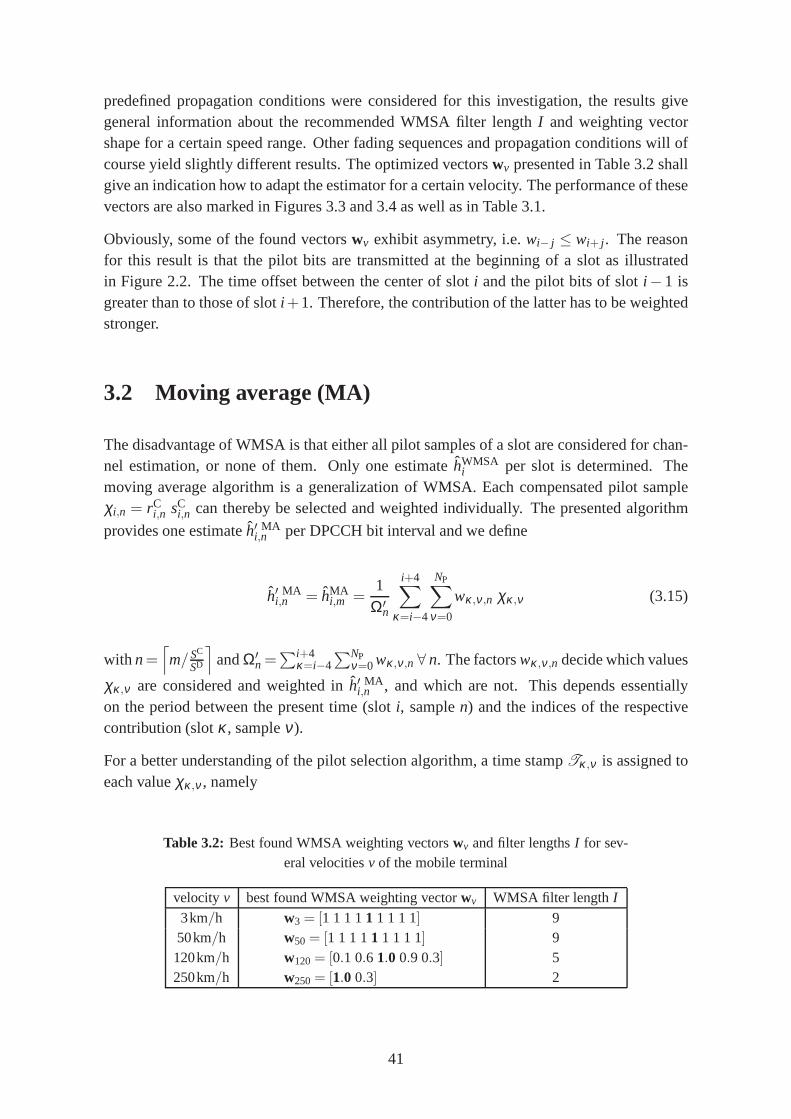
predefined propagation conditions were considered for thisinvestigation, the results givegeneral information about the recommended WMSA filter length I and weighting vectorshape for a certain speed range. Other fading sequences and propagation conditions will ofcourse yield slightly different results. The optimized vectorswv presented in Table 3.2 shallgive an indication how to adapt the estimator for a certain velocity. The performance of thesevectors are also marked in Figures 3.3 and 3.4 as well as in Table 3.1.

Obviously, some of the found vectorswv exhibit asymmetry, i.e.wi− j ≤ wi+ j . The reasonfor this result is that the pilot bits are transmitted at the beginning of a slot as illustratedin Figure 2.2. The time offset between the center of sloti and the pilot bits of sloti −1 isgreater than to those of sloti +1. Therefore, the contribution of the latter has to be weightedstronger.

3.2 Moving average (MA)

The disadvantage of WMSA is that either all pilot samples of aslot are considered for chan-nel estimation, or none of them. Only one estimatehWMSA

i per slot is determined. Themoving average algorithm is a generalization of WMSA. Each compensated pilot sampleχi,n = rC

i,n sCi,n can thereby be selected and weighted individually. The presented algorithm

provides one estimateh′ MAi,n per DPCCH bit interval and we define

h′ MAi,n = hMA

i,m =1

Ω′n

i+4∑

κ=i−4

NP∑

ν=0

wκ,ν,n χκ,ν (3.15)

with n=⌈

m/SC

SD

⌉

andΩ′n =∑i+4

κ=i−4∑NP

ν=0wκ,ν,n ∀ n. The factorswκ,ν,n decide which values

χκ,ν are considered and weighted inh′ MAi,n , and which are not. This depends essentially

on the period between the present time (sloti, samplen) and the indices of the respectivecontribution (slotκ , sampleν).

For a better understanding of the pilot selection algorithm, a time stampTκ,ν is assigned toeach valueχκ,ν , namely

Table 3.2: Best found WMSA weighting vectorswv and filter lengthsI for sev-eral velocitiesv of the mobile terminal

velocity v best found WMSA weighting vectorwv WMSA filter lengthI

3km/h w3 = [1 1 1 11 1 1 1 1] 950km/h w50 = [1 1 1 11 1 1 1 1] 9120km/h w120 = [0.1 0.6 1.0 0.9 0.3] 5250km/h w250 = [1.0 0.3] 2

41

Tκ,ν = 10· (κ − i +4)+ν, (3.16)

wherei−4≤ κ ≤ i +4 and 1≤ ν ≤NP. Thus,Tκ,ν can take the values 1,2, . . . ,NP,11,12, . . .10+NP, . . . ,81,82, . . . ,80+NP. The present timePn is defined as

Pn = 40+n 1≤ n≤ 10. (3.17)

Each valueχκ,ν is characterized by a time offset

∆κ,ν,n = Tκ,ν −Pn(3.16,3.17)

= 10(κ − i)+ν −n, (3.18)

also depending on the time indexn.∣

∣∆κ,ν,n∣

∣ is a measure for the lag between the presenttime and the reception of the respective pilot sample. As thechannel is time-variant, it isadvantageous to select thoseχκ,ν for channel estimation that exhibit the smallest

∣

∣∆κ,ν,n∣

∣.Figure 3.5 presents the moving average algorithm accordingto (3.15) and clarifies the timestampsTκ,ν .

In the following, we will restrict to the special casewκ,ν,n ∈ 0,1, i.e.Ω′n is the number of

considered valuesχκ,ν , also referred to as moving average filter length. The pilot selectionalgorithm that determineswκ,ν,n is illustrated in Figure 3.6. A target filter lengthΩ is givenas parameter. Primarily, for eachn theΩ valuesχκ,ν with the smallest time lag

∣

∣∆κ,ν,n∣

∣ areselected. For an optimal channel tracking, the mean of thesevalues∆κ,ν,n must be as smallas possible. This criterion can be checked with the helper variableG. If |G| ≤Ω/2, the pilotsreceived before and after the present time are well balanced, and a further optimization is notnecessary. Otherwise, one pilot sample either at the beginning or at the end of the selectionis possibly also considered in order to fulfill this side condition. For this purpose, the sumsGandG′ are compared. Hence it follows thatΩ′

n ∈ Ω,Ω+1. For the caseΩ > 9·NP−2, anexception handling has to be executed that is left out in Figure 3.6. An alternative solutionis the removal of one pilot sample at one border of the filter. Also both approaches can becombined.

Computer simulation has shown that this sophisticated pilot selection algorithm is superiorto the basic solution with a fixed filter length. For an effective implementation of the movingaverage on a digital signal processor, sets of weighting factors wκ,ν,n for useful valuesΩcould be stored in a look-up table. Nevertheless, the complexity of moving average is highercompared to WMSA.

Optimal valuesΩv in terms of smallest BLER after decoding were determined forthe veloci-tiesv= 50,120 and 250km/h by computer simulation with the parameters from Appendix B.With NP = 6, the maximal possible target filter length isΩ = 54. Figures 3.7 and 3.8 showthe results atEb/N0 = 2.0dB andEb/N0 = 2.6dB, respectively.

In Figure 3.7, we findΩ50 = 51 as optimal target filter length for 50km/h, whereas thehigher velocity 120km/h requires withΩ120 = 24 a shorter channel observation time. Fi-nally, at 250km/h the very fast changing channel conditions force a further reduction of the

42

? ? ? ? ? ?-

-CE inputshift register

time-stampTκ,ν

1 NP 11 70+NP 81 80+NP

χi−4,1 · · · χi−4,NP χi−3,1 · · · χi+3,NP χi+4,1 · · · χi+4,NP

wi−4,1,n · · · wi−4,NP,n wi−3,1,n · · · wi+3,NP,n wi+4,1,n · · · wi+4,NP,n

∑

1Ω′

n

h′ MAi,n

Figure 3.5: Implementation model of the moving average algorithm

for n = 1, . . . ,10

w′∆κ,ν,n

= wκ,ν ,n = 0

A =

∣

∣∆κ,ν ,n∣

∣

in ascending order

B = A (1, . . . ,Ω+2)

C =

∆κ,ν ,n

∣

∣

∣

∣

∣∆κ,ν ,n∣

∣ ∈ B

in ascending order

G =∑Ω+1

i=2 C (i)

w′C (i) = 1 i = 2, . . . ,Ω+1

G > Ω2 ?

yes no

G′ = G+C (1)∣

∣G′∣∣< |G|?

yes no

w′C (1) = 1

G < −Ω2 ?

yes no

G′ = G+C (Ω+2)∣

∣G′∣∣< |G|?

yes no

w′C (Ω+2) = 1

wκ,ν ,n = w′∆κ,ν,n

Figure 3.6: Pilot selection algorithm for moving average

43

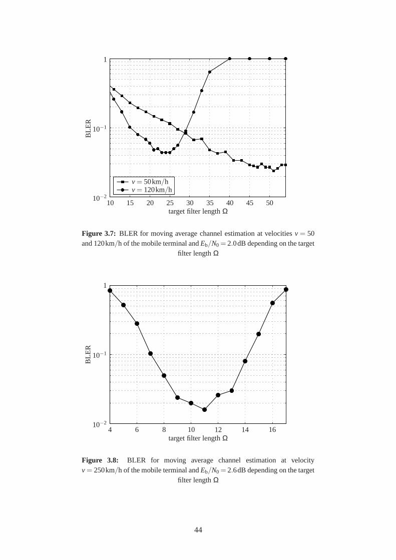
v = 50 km/hv = 120 km/h

10 15 20 25 30 35 40 45 50target filter lengthΩ

10−2

10−1

1

BL

ER

v = 50km/hv = 120km/h

Figure 3.7: BLER for moving average channel estimation at velocitiesv = 50and 120km/h of the mobile terminal andEb/N0 = 2.0dB depending on the target

filter lengthΩ

4 6 8 10 12 14 16target filter lengthΩ

10−2

10−1

1

BL

ER

Figure 3.8: BLER for moving average channel estimation at velocityv = 250km/h of the mobile terminal andEb/N0 = 2.6dB depending on the target

filter lengthΩ

44

filter length to yield appropriate results. According to Figure 3.8, the best found value isΩ250= 11. For the same reason as for WMSA, the optimal target filter lengthΩv becomessmaller with increasing velocityv.

3.3 WMSA and moving average with interpolation

The WMSA algorithm determines only one channel estimatehWMSAi . This is sufficient if

the channel is only changing slowly, i.e. at low speed of the mobile terminal. However, forsome DPDCH samplesm WMSA may cause a significant estimation errorei,m and phaseerror ϕi,m. Concerning this, the moving average algorithm is an improvement. It providesone estimateh′ MA

i,n per DPCCH bit interval. But the spreading factorSD of the DPDCH issmaller than that of the DPCCH (SC = 256). Several DPDCH samples are received duringone DPCCH bit interval. For very high speed, the channel changes noticeably during thistime. In order to reduceei,m andϕi,m, an interpolation between the estimates can be applied.Finally, each DPDCH sample will get its individual estimatehi,m.

Firstly, the interpolation algorithm for WMSA is presented. If the elementswκ of the WMSAweighting vectorw are shifted one position to the right, (3.13) determines theestimatehWMSA

i+1 of the sloti +1. As an example, the vectorw = [0.0 0.0 0.1 0.6 1.0 0.9 0.3 0.0 0.0]

becomesw = [0.0 0.0 0.0 0.1 0.6 1.0 0.9 0.3 0.0]. Moreover, we assume that the previousestimateshWMSA

i−1 andhWMSAi are still available. The mean values

θ1 =12

(

hWMSAi−1 + hWMSA

i

)

(3.19)

and

θ2 =12

(

hWMSAi + hWMSA

i+1

)

(3.20)

are the border points of the interpolation within sloti. The interpolated values are

hWMSA-Ii,m = θ1+

2m−12

·∆h m= 1, . . . ,M (3.21)

with ∆h = (θ2−θ1)/M. Figure 3.9 illustrates (3.19), (3.20) and (3.21). If the dotted linerepresents the actual channel, the estimation errorei,m is significantly decreased. Moreover,the algorithm reduces the impact of noise better than the original WMSA because the pilotsamples of an additional slot are considered due to the shiftoperation inw.

If moving average is used as basic channel estimation algorithm, each interpolation coversone DPCCH bit interval with the border points

45

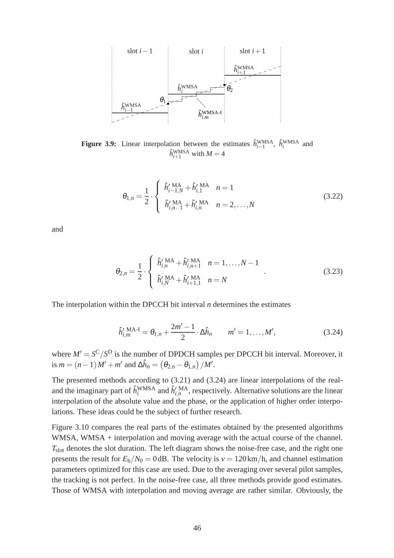
slot i −1 slot i slot i +1

hWMSAi−1

hWMSAi

hWMSAi+1

θ1

θ2

hWMSA-Ii,m

Figure 3.9: Linear interpolation between the estimateshWMSAi−1 , hWMSA

i andhWMSA

i+1 with M = 4

θ1,n =12·

h′ MAi−1,N + h′ MA

i,1 n = 1

h′ MAi,n−1+ h′ MA

i,n n = 2, . . . ,N(3.22)

and

θ2,n =12·

h′ MAi,n + h′ MA

i,n+1 n = 1, . . . ,N−1

h′ MAi,N + h′ MA

i+1,1 n = N. (3.23)

The interpolation within the DPCCH bit intervaln determines the estimates

h′ MA-Ii,m = θ1,n+

2m′−12

·∆hn m′ = 1, . . . ,M′, (3.24)

whereM′ = SC/SD is the number of DPDCH samples per DPCCH bit interval. Moreover, itis m= (n−1)M′+m′ and∆hn =

(

θ2,n−θ1,n)

/M′.

The presented methods according to (3.21) and (3.24) are linear interpolations of the real-and the imaginary part ofhWMSA

i andh′ MAi,n , respectively. Alternative solutions are the linear

interpolation of the absolute value and the phase, or the application of higher order interpo-lations. These ideas could be the subject of further research.

Figure 3.10 compares the real parts of the estimates obtained by the presented algorithmsWMSA, WMSA + interpolation and moving average with the actual course of the channel.Tslot denotes the slot duration. The left diagram shows the noise-free case, and the right onepresents the result forEb/N0 = 0dB. The velocity isv = 120km/h, and channel estimationparameters optimized for this case are used. Due to the averaging over several pilot samples,the tracking is not perfect. In the noise-free case, all three methods provide good estimates.Those of WMSA with interpolation and moving average are rather similar. Obviously, the

46

actual channelWMSAWMSA + interpolationmoving average

0 2 4 6relative timet/Tslot

−0.2

−0.1

0.0

0.1

0.2

0.3ℜ

ampl

itude

(a)

actual channelWMSAWMSA + interpolationmoving average

0 2 4 6relative timet/Tslot

−0.2

−0.1

0.0

0.1

0.2

0.3

ℜ

ampl

itude

(b)

Figure 3.10: Comparison of channel estimates obtained with WMSA, WMSA+ interpolation and moving average in comparison to the actual channel coeffi-

cients (a) in the noise-free case and (b) atEb/N0 = 0dB

interpolation is not always advantageous. As an example, atthe beginning of the third slotWMSA causes the smallest estimation error.

In the presence of noise, the estimation error of all methodsis noticeably increased. Dia-gram 3.10b shall exemplify the behavior of the algorithms. However, a rating based on thecourses is not possible. Any resemblance to a phase shift between the actual channel and theestimates is purely coincidental.

Also the mean phase error∣

∣ϕi,m∣

∣ was measured for the proposed methods. The results forselected velocities in the noise-free case and forEb/N0 = 0dB are given in Table 3.3. Untilv = 120km/h, the values are rather similar. At 250km/h moving average based channel es-timation yields a clear performance gain compared to WMSA. However, the more importantmeasurements are the bit- and block error ratios to be discussed in the next chapter.

3.4 BER and BLER performance evaluation

Finally, the performance in terms of bit error ratio (BER) and block error ratio (BLER)of the proposed algorithms was measured by computer simulation for several velocitiesvof the mobile terminal. Appendix B presents tables with all used parameters. Always theoptimized channel estimation parametersw for WMSA and Ω for moving average wereselected. The following figures also include the performance of the "ideal" channel estimatoras a benchmark for the achieved results.

47

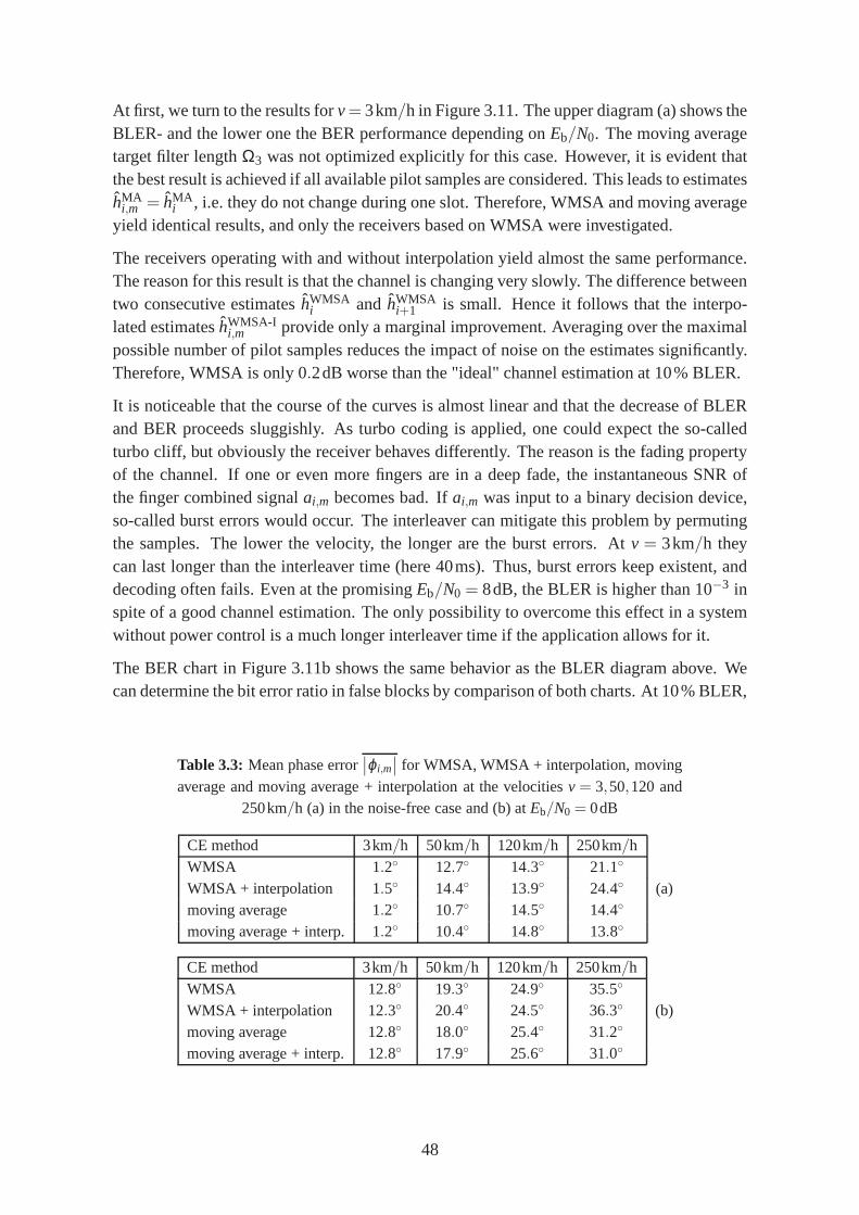
At first, we turn to the results forv= 3km/h in Figure 3.11. The upper diagram (a) shows theBLER- and the lower one the BER performance depending onEb/N0. The moving averagetarget filter lengthΩ3 was not optimized explicitly for this case. However, it is evident thatthe best result is achieved if all available pilot samples are considered. This leads to estimateshMA

i,m = hMAi , i.e. they do not change during one slot. Therefore, WMSA andmoving average

yield identical results, and only the receivers based on WMSA were investigated.

The receivers operating with and without interpolation yield almost the same performance.The reason for this result is that the channel is changing very slowly. The difference betweentwo consecutive estimateshWMSA

i and hWMSAi+1 is small. Hence it follows that the interpo-

lated estimateshWMSA-Ii,m provide only a marginal improvement. Averaging over the maximal

possible number of pilot samples reduces the impact of noiseon the estimates significantly.Therefore, WMSA is only 0.2dB worse than the "ideal" channel estimation at 10% BLER.

It is noticeable that the course of the curves is almost linear and that the decrease of BLERand BER proceeds sluggishly. As turbo coding is applied, onecould expect the so-calledturbo cliff, but obviously the receiver behaves differently. The reason is the fading propertyof the channel. If one or even more fingers are in a deep fade, the instantaneous SNR ofthe finger combined signalai,m becomes bad. Ifai,m was input to a binary decision device,so-called burst errors would occur. The interleaver can mitigate this problem by permutingthe samples. The lower the velocity, the longer are the bursterrors. Atv = 3km/h theycan last longer than the interleaver time (here 40ms). Thus,burst errors keep existent, anddecoding often fails. Even at the promisingEb/N0 = 8dB, the BLER is higher than 10−3 inspite of a good channel estimation. The only possibility to overcome this effect in a systemwithout power control is a much longer interleaver time if the application allows for it.

The BER chart in Figure 3.11b shows the same behavior as the BLER diagram above. Wecan determine the bit error ratio in false blocks by comparison of both charts. At 10% BLER,

Table 3.3: Mean phase error∣

∣ϕi,m∣

∣ for WMSA, WMSA + interpolation, movingaverage and moving average + interpolation at the velocities v = 3,50,120 and

250km/h (a) in the noise-free case and (b) atEb/N0 = 0dB

CE method 3km/h 50km/h 120km/h 250km/hWMSA 1.2 12.7 14.3 21.1

WMSA + interpolation 1.5 14.4 13.9 24.4 (a)moving average 1.2 10.7 14.5 14.4

moving average + interp. 1.2 10.4 14.8 13.8

CE method 3km/h 50km/h 120km/h 250km/hWMSA 12.8 19.3 24.9 35.5

WMSA + interpolation 12.3 20.4 24.5 36.3 (b)moving average 12.8 18.0 25.4 31.2

moving average + interp. 12.8 17.9 25.6 31.0

48

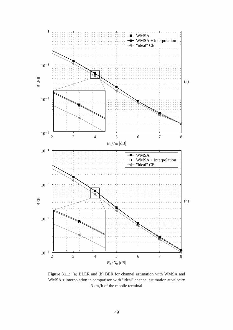
WMSAWMSA + interpolation"ideal" CE

2 3 4 5 6 7 8

Eb/N0 [dB]

10−3

10−2

10−1

1

BL

ER

(a)

WMSAWMSA + interpolation"ideal" CE

2 3 4 5 6 7 8

Eb/N0 [dB]

10−4

10−3

10−2

10−1

BE

R (b)

Figure 3.11: (a) BLER and (b) BER for channel estimation with WMSA andWMSA + interpolation in comparison with "ideal" channel estimation at velocity

3km/h of the mobile terminal

49

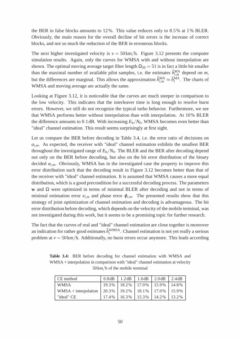
the BER in false blocks amounts to 12%. This value reduces only to 8.5% at 1% BLER.Obviously, the main reason for the overall decline of bit errors is the increase of correctblocks, and not so much the reduction of the BER in erroneous blocks.

The next higher investigated velocity isv = 50km/h. Figure 3.12 presents the computersimulation results. Again, only the curves for WMSA with andwithout interpolation areshown. The optimal moving average target filter lengthΩ50 = 51 is in fact a little bit smallerthan the maximal number of available pilot samples, i.e. theestimateshMA

i,m depend onm,

but the differences are marginal. This allows the approximation hMAi,m ≈ hMA

i . The charts ofWMSA and moving average are actually the same.

Looking at Figure 3.12, it is noticeable that the curves are much steeper in comparison tothe low velocity. This indicates that the interleaver time is long enough to resolve bursterrors. However, we still do not recognize the typical turbobehavior. Furthermore, we seethat WMSA performs better without interpolation than with interpolation. At 10% BLERthe difference amounts to 0.1dB. With increasingEb/N0, WMSA becomes even better than"ideal" channel estimation. This result seems surprisingly at first sight.

Let us compare the BER before decoding in Table 3.4, i.e. the error ratio of decisions onai,m. As expected, the receiver with "ideal" channel estimationexhibits the smallest BERthroughout the investigated range ofEb/N0. The BLER and the BER after decoding dependnot only on the BER before decoding, but also on the bit error distribution of the binarydecidedai,m. Obviously, WMSA has in the investigated case the property to improve thiserror distribution such that the decoding result in Figure 3.12 becomes better than that ofthe receiver with "ideal" channel estimation. It is assumedthat WMSA causes a more equaldistribution, which is a good precondition for a successfuldecoding process. The parametersw and Ω were optimized in terms of minimal BLER after decoding and not in terms ofminimal estimation errorei,m and phase errorϕi,m. The presented results show that thisstrategy of joint optimization of channel estimation and decoding is advantageous. The biterror distribution before decoding, which depends on the velocity of the mobile terminal, wasnot investigated during this work, but it seems to be a promising topic for further research.

The fact that the curves of real and "ideal" channel estimation are close together is moreoveran indication for rather good estimateshWMSA

i . Channel estimation is not yet really a seriousproblem atv = 50km/h. Additionally, no burst errors occur anymore. This leads according

Table 3.4: BER before decoding for channel estimation with WMSA andWMSA + interpolation in comparison with "ideal" channel estimation at velocity

50km/h of the mobile terminal

CE method 0.8dB 1.2dB 1.6dB 2.0dB 2.4dB

WMSA 19.3% 18.2% 17.0% 15.9% 14.8%WMSA + interpolation 20.3% 19.2% 18.1% 17.0% 15.9%"ideal" CE 17.4% 16.3% 15.3% 14.2% 13.2%

50

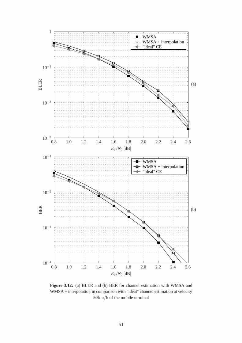
WMSAWMSA + interpolation"ideal" CE

0.8 1.0 1.2 1.4 1.6 1.8 2.0 2.2 2.4 2.6

Eb/N0 [dB]

10−3

10−2

10−1

1

BL

ER

(a)

WMSAWMSA + interpolation"ideal" CE

0.8 1.0 1.2 1.4 1.6 1.8 2.0 2.2 2.4 2.6

Eb/N0 [dB]

10−4

10−3

10−2

10−1

BE

R

(b)

Figure 3.12: (a) BLER and (b) BER for channel estimation with WMSA andWMSA + interpolation in comparison with "ideal" channel estimation at velocity

50km/h of the mobile terminal

51

to Figure 3.3 to the smallest requiredEb/N0 to achieve a BLER of 10%.

The BER chart in Figure 3.12b shows a similar behavior as the BLER diagram above. Thedifference between WMSA with and without interpolation also amounts to 0.1dB. UsingWMSA without interpolation, the BER in false blocks is about4% at 10% BLER. Thisvalue decreases slightly to 2.5% at 1% BLER. The BER in false blocks is smaller comparedto the low speed casev = 3km/h

Let us now consider Figure 3.13, presenting the results forv = 120km/h. The curves havebecome even more steep than before. Now, WMSA with interpolation is the algorithm thatyields the best performance. It is just the other way round compared to the casev = 50km/h.The gain towards WMSA without interpolation is about 0.1dB at 10% BLER. The movingaverage receivers with and without interpolation perform almost equal. Their BLER curvesrun between those of the WMSA based receivers. The offset to "ideal" channel estimationhas become bigger. It amounts to 0.4dB for WMSA with interpolation. This indicates thatchannel estimation is a serious topic forv = 120km/h. It requires a careful selection of theparameters. Otherwise, the SNR of the decoder inputai,m becomes too bad, and the BLERincreases siginificantly.

The BER chart in Figure 3.13b behaves again similar as the BLER diagram above. Consid-ering the best algorithm, WMSA with interpolation, we find 2.5% BER in false blocks at10% BLER and about 2% BER at 1% BLER. This is a further BER reduction compared topreviously presented results for lower speeds.

The highest velocity that was investigated isv = 250km/h. Figure 3.14a shows the BLERperformance of the four presented channel estimation algorithms, and Figure 3.14b belowpresents the respective BER curves. Among all discussed diagrams, we recognize here mostclearly a turbo cliff. The BLER curves decrease steeply fromEb/N0 = 2dB after a flat coursebefore. The reason is that the bit errors before decoding show most clearly an equal distri-bution compared to the cases with lower speed. Now, the moving average based algorithmsperform about 0.4dB better than WMSA at 10% BLER. The methods with interpolationprovide a small improvement in each case. In comparison tov = 120km/h, the offset to"ideal" channel estimation has increased to 1.2dB. The fast changing channel requires op-timal selected parameters. Channel estimation at high speed of the mobile terminal is a bigchallenge for the receiver.

For moving average with interpolation, the BER in false blocks amounts to 2% at 10%BLER and a bit less at 1% BLER. These values are in the same range as for the casev = 120km/h. Generally, it was found out that the BER in false blocks reduces if the ve-locity of the terminal increases. Knowledge of the BER in erroneous blocks is important forapplications not operating with re-transmission of those blocks, but applying an outer errorprotection, e.g. Reed-Solomon coding [35], to correct remaining bit errors. An importantexample for such an application is video broadcast.

52

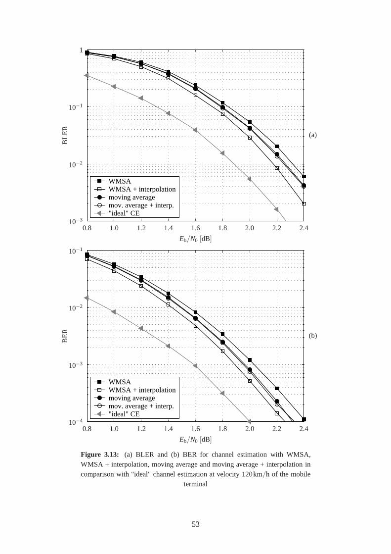
WMSAWMSA + interpolationmoving averagemov. average + interp."ideal" CE

0.8 1.0 1.2 1.4 1.6 1.8 2.0 2.2 2.4

Eb/N0 [dB]

10−3

10−2

10−1

1

BL

ER

(a)

WMSAWMSA + interpolationmoving averagemov. average + interp."ideal" CE

0.8 1.0 1.2 1.4 1.6 1.8 2.0 2.2 2.4

Eb/N0 [dB]

10−4

10−3

10−2

10−1

BE

R

(b)

Figure 3.13: (a) BLER and (b) BER for channel estimation with WMSA,WMSA + interpolation, moving average and moving average + interpolation incomparison with "ideal" channel estimation at velocity 120km/h of the mobile

terminal

53

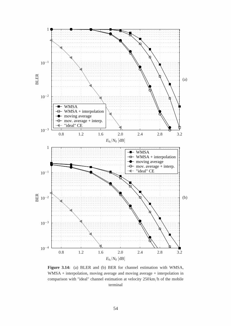
WMSAWMSA + interpolationmoving averagemov. average + interp."ideal" CE

0.8 1.2 1.6 2.0 2.4 2.8 3.2

Eb/N0 [dB]

10−3

10−2

10−1

1

BL

ER

(a)

WMSAWMSA + interpolationmoving averagemov. average + interp."ideal" CE

0.8 1.2 1.6 2.0 2.4 2.8 3.2

Eb/N0 [dB]

10−4

10−3

10−2

10−1

1

BE

R

(b)

Figure 3.14: (a) BLER and (b) BER for channel estimation with WMSA,WMSA + interpolation, moving average and moving average + interpolation incomparison with "ideal" channel estimation at velocity 250km/h of the mobile

terminal

54

Chapter 4

Channel estimation with rake feedback

Several channel estimation algorithms based on the pilot samplesrCl ,i,n (n = 1, . . . ,NP) have

been discussed.l indicates the rake fingers. Figure 2.14 shows the block diagram of therespective receiver. An extension of this conventional design is the introduction of feedbackloops that also allow to utilize the non-pilot samplesrC

l ,i,n (n= NP+1, . . . ,10) of the DPCCHandrD

l ,i,m of the DPDCH for channel estimation. Several options for feedback assisted chan-nel estimation for WCDMA are discussed in the literature, e.g. [33] and [36]. Generally, thefeedback of the DPDCH can be applied before or after decoding. In the first case, the feed-back loop is part of the rake receiver. Therefore, this approach is denoted asrake feedbackin the following. Several implementations of rake feedbackare investigated in this chapter,whereas the next chapter will deal with feedback after decoding. All presented methods useWMSA as basic channel estimation algorithm.

4.1 DPCCH rake feedback

Firstly, the receiver in Figure 4.1 is presented. It exploits the non-pilot samples of theDPCCH for channel estimation. As before, a first channel estimation based on the pilotsamplesrC

l ,i,n (n = 1, . . . ,NP) is carried out. These estimates are denoted ash1,l ,i and areinput to a DPCCH maximum ratio combiner. Hence, the switch S1is initially in the upperposition. MRC is applied to the samplesrC

l ,i,n, and we yield

aCi,n =

L∑

l=1

rCl ,i,n h∗1,l ,i, (4.1)

wheren= NP+1, . . . ,10. Note that all MRCs used for rake feedback are defined without thereal part operation from (2.36), i.e. their outputsaC

i,n andaD1,i,m are complex. In the following,

we will restrict to one rake finger and skip indexl to simplify matters.

ConsideringaCi,n, the instantaneous channel estimateχi from (3.13) shall be replaced by an

improved valueχ ′i , namely

55

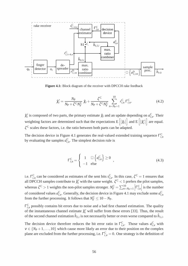
rake receiver

-qh

fingerdetector

-oc

de-spreader -

rDl ,i,m

max.ratio

combiner-

ℜ

aD1,i,m

sampleproc.

-bν ,k

rCl ,i+4,n

--

sCi+4,n

channelestimator

?h2,l ,i

-max.ratio

combiner

h1,l ,i ?aC

i,n

decisiondevice

ΓC

i,n

S1

Figure 4.1: Block diagram of the receiver with DPCCH rake feedback

χ ′i =

NP

NP+ζ CNCF

χi +ζ C

NP+ζ CNCF

10∑

n=NP+1

rCi,n ΓC

i,n. (4.2)

χ ′i is composed of two parts, the primary estimateχi and an update depending onaC

i,n. Their

weighting factors are determined such that the expectations E[

∣

∣χi∣

∣

]

and E[

∣

∣χ ′i

∣

∣

]

are equal.

ζ C scales these factors, i.e. the ratio between both parts can be adapted.

The decision device in Figure 4.1 generates the real-valuedextended training sequenceΓCi,n

by evaluating the samplesaCi,n. The simplest decision rule is

ΓCi,n =

1 ℜ

aCi,n

≥ 0

−1 else, (4.3)

i.e. ΓCi,n can be considered as estimates of the sent bitssC

i,n. In this case,ζ C = 1 ensures thatall DPCCH samples contribute toχ ′

i with the same weight.ζ C < 1 prefers the pilot samples,

whereasζ C > 1 weights the non-pilot samples stronger.NCF =

∑10n=NP+1

∣

∣

∣ΓC

i,n

∣

∣

∣is the number

of considered valuesaCi,n. Generally, the decision device in Figure 4.1 may exclude someaC

i,n

from the further processing. It follows thatNCF ≤ 10−NP.

ΓCi,n possibly contains bit errors due to noise and a bad first channel estimation. The quality

of the instantaneous channel estimateχ ′i will suffer from these errors [33]. Thus, the result

of the second channel estimationh2,i is not necessarily better or even worse compared toh1,i .

The decision device therefore reduces the bit error ratio inΓCi,n. Those valuesaC

i,ν withν ∈ NP+1, . . . ,10 which cause more likely an error due to their position on the complexplane are excluded from the further processing, i.e.ΓC

i,ν = 0. One strategy is the definition of

56

thresholds parallel to the imaginary axis, i.e.∣

∣

∣ℜ

aCi,n

∣

∣

∣has to exceed a certain value. How-

ever, computer simulation has shown that a decision upon thephase arc

aCi,n

is superior.

The two thresholds in Figure 4.2 and the real axis include theangleψC. The decision deviceexcludes all valuesaC

i,n in the gray area. This leads to the rule

ΓCi,n =

+1 −ψC ≤ arc

aCi,n

≤ ψC

−1 arc

aCi,n

≥ π −ψC or arc

aCi,n

≤−π +ψC

0 else

. (4.4)

Channel estimatesh2,i based on DPCCH rake feedback are finally determined as

h2,i =1

∑i+4κ=i−4wC

κ

i∑

κ=i−4

wCκ χ ′

κ +

i+4∑

κ=i+1

wCκ χκ

. (4.5)

wCκ are elements of a WMSA weighting vector used for the second channel estimation. (4.5)

takes into consideration that updatesχ ′κ are only available for the present and past slots

κ = i − 4, . . . , i, whereas for the future slotsκ = i + 1, . . . , i + 4 the original instantaneousestimatesχκ have to be re-used. The switch S1 leadsh2,i to the DPDCH MRC that detectsthe finger combined samplesaD

1,i,m.

According to the feedback threshold angleψC, more or less valuesaCi,n are considered for

the second channel estimation.ψC = π2 is equivalent to (4.3).ψC was optimized in terms of

minimal BLER after decoding by computer simulation. The velocity of the mobile terminalwas set tov = 250km/h because this case is most demanding for the receiver. The result ispresented in Figure 4.3. Obviously, the best found angle isψC = 80. DecreasingψC causesa significant higher BLER. ForψC ≤ 10 the result becomes even worse compared to thereceiver without rake feedback. The reason for this behavior is the used WMSA weightingvector wC

250 from Table 4.1. It was optimized forψC = 80. It was found out that thiscombination of both parameters yields the best result.

Table 4.1 also presents an optimized WMSA weighting vectorwC120 for v = 120km/h. In

contrast to the vectorswv from Table 3.2, which are used for the first channel estimation, thenew vectors exhibit symmetry. As the receiver with rake feedback also partly exploits thenon-pilot bits of the DPCCH for channel estimation, is it notnecessary to keep the unequalslot weights.

Finally, the impact of the feedback scaling factorζ C on the BLER after decoding was in-

vestigated. According to Figure 4.4, 20· log(

ζ C)

= 0dB, i.e.ζ C = 1 provides the best

57

-

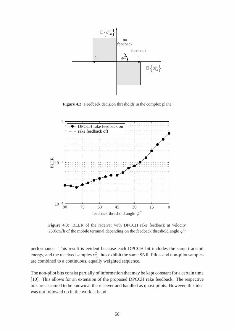
6

IψC

ℜ

aCi,n

ℑ

aCi,n

−1 1

nofeedback

feedback

Figure 4.2: Feedback decision thresholds in the complex plane

DPCCH rake feedback onrake feedback off

90 75 60 45 30 15 0

feedback threshold angleψC

10−2

10−1

1

BL

ER

Figure 4.3: BLER of the receiver with DPCCH rake feedback at velocity250km/h of the mobile terminal depending on the feedback thresholdangleψC

performance. This result is evident because each DPCCH bit includes the same transmitenergy, and the received samplesrC

i,n thus exhibit the same SNR. Pilot- and non-pilot samplesare combined to a continuous, equally weighted sequence.

The non-pilot bits consist partially of information that may be kept constant for a certain time[10]. This allows for an extension of the proposed DPCCH rakefeedback. The respectivebits are assumed to be known at the receiver and handled as quasi-pilots. However, this ideawas not followed up in the work at hand.

58

DPCCH rake feedback onrake feedback off

−16 −12 −8 −4 0 4 8 12 16

feedback scaling factor 20· log(

ζ C)

[dB]

10−2

10−1

1

BL

ER

Figure 4.4: BLER of the receiver with DPCCH rake feedback at velocity250km/h of the mobile terminal depending on the feedback scaling factor ζ C

4.2 DPDCH rake feedback

Similar to the feedback of non-pilot bits of the DPCCH, also the DPDCH samplesrDi,m can

be exploited for a second channel estimation. Figure 4.5 shows the block diagram of thisreceiver.

Firstly, the channel estimator provides estimatesh1,i based on pilot bits, which are input tothe MRC. The switch S2 is in the upper position, and the finger combined outputaD

1,i,m is fedback to a decision device. According to a decision rule, an extended training sequenceΓD

i,m isformed. The channel estimator utilizesΓD

i,m to update the instantaneous channel estimateχi .

After the WMSA algorithm was applied again, improved channel estimatesh2,i are available.Also the outputaD

2,i,m from the second MRC operation profits by the more accurate estimates.

The switch S2 is now in the lower position, andℜ

aD2,i,m

is input to the sample processingmodule. The BLER is reduced compared with the receiver without DPDCH rake feedback.

Equivalent to the DPCCH rake feedback decision rule (4.4), the extended training sequence

Table 4.1: Best found WMSA weighting vectorswCv for DPCCH rake feedback

channel estimation for the velocities 120 and 250km/h of the mobile terminal

velocity v WMSA weighting vectorwCv

120km/h wC120 = [0.4 0.8 1.0 0.8 0.4]

250km/h wC250 = [0.2 1.0 0.2]

59

rake receiver

-qh

fingerdetector

-oc

de-spreader -

rDi,m

max.ratio

combiner-

ℜ

aD2,i,m

sampleproc.

-bν ,k

rCi+4,n

--

sCi+4,n

channelestimator

?

h1,ih2,i

aD1,i,m

decisiondevice

ΓD

i,m

?S2

Figure 4.5: Block diagram of the receiver with DPDCH rake feedback

ΓDi,m is built up under consideration of the phase of the MRC outputaD

1,i,m, i.e.

ΓDi,m =

+1 −ψD ≤ arc

aD1,i,m

≤ ψD

−1 arc

aD1,i,m

≥ π −ψD or arc

aD1,i,m

≤−π +ψD

0 else

, (4.6)

whereψD is the feedback threshold angle according to Figure 4.2.ψD was optimized underthe same conditions asψC before. Figure 4.6 shows thatψD = 85 leads to the lowest BLERfor the velocityv= 250km/h. We see a quite similar impact of the threshold angleψD on theBLER as it was found out for its counterpartψC in the previous chapter. A measurement of

the ratioNDF /M in Table 4.3 exemplifies the effect ofψD. ND

F =∑M

m=1

∣

∣

∣ΓD

i,m

∣

∣

∣is the number

of elements unequal zero inΓDi,m.

Table 4.2 presents the optimized WMSA weighting vectorswD120 andwD

250. Obviously, theWMSA filter length used for the DPDCH rake feedback channel estimation is significantlyreduced compared to the first estimation and DPCCH rake feedback. We have seen in Chap-ter 3 that without noise the filter lengthI = 1 shows the best tracking of the channel. Theonly reason forI > 1 is the necessity of noise suppression by averaging over many compen-sated pilot samplesχκ,n. As the DPDCH normally is transmitted with a higher power portion

Table 4.2: Best found WMSA weighting vectorswDv for DPDCH rake feedback

channel estimation for the velocities 120 and 250km/h of the mobile terminal

velocity v WMSA weighting vectorwDv

120km/h wD120 = [0.1 1.0 0.1]

250km/h wD250 = [1.0]

60

DPDCH rake feedback onrake feedback off

90 75 60 45 30 15 0

feedback threshold angleψD

10−2

10−1

1

BL

ER

Figure 4.6: BLER of the receiver with DPDCH rake feedback at velocity250km/h of the mobile terminal depending on the feedback thresholdangleψD

(γ < 0dB), the use of the extended training sequenceΓDi,m reduces the impact of noise onh2,i

effectively. A considerable extension of the channel observation timeTobs is not requiredanymore.

The updateχ ′i of the instantaneous channel estimateχi is given as

χ ′i = ϒ

(

χi +ζ D

NDF

M∑

m=1

rDi,m ΓD

i,m

)

, (4.7)

where the factor

ϒ =SC

SC+ζ D SD 10γ/20

√MP

(4.8)

guarantees that the expectations E[

∣

∣χi∣

∣

]

and E[

∣

∣χ ′i

∣

∣

]

are equal. The scaling factorζ D con-

trols the ratio between pilot bitssCi,n and extended training sequenceΓD

i,m in the same way as

Table 4.3: PortionNDF /M of considered fed back samplesaD

1,i,m depending on thethreshold angleψD atv = 250km/h of the mobile terminal andEb/N0 = 2.2dB

ψD 90 80 70 60 50 40 30 20 10 0

NDF

M 100% 92.3% 84.3% 75.6% 66.0% 55.1% 43.0% 29.5% 15.1% 0%

61

ζ C for DPCCH rake feedback.

The channel estimatesh2,i are finally determined as

h2,i =1

∑i+4κ=i−4wD

κ

i∑

κ=i−4

wDκ χ ′

κ +

i+4∑

κ=i+1

wDκ χκ

. (4.9)

Updated instantaneous estimatesχ ′κ are only available for the present slotκ = i and the past

slotsκ = i −4, . . . , i −1. For the future slotsκ = i +1, . . . , i +4 the original valuesχκ haveto be re-used.

The impact of the scaling factorζ D on the BLER after decoding was investigated by com-puter simulation with the parameters from Appendix B. The velocity was set to 250km/h.Figure 4.7 presents the result of this optimization. In the left part of the diagram, the extendedtraining sequenceΓD

i,m has only little influence onχ ′i . The very short WMSA weighting vec-

tor wD250 is inappropriate for this case, and rake feedback degrades the performance of the

receiver. The moreζ D is increased, the lower becomes the BLER, finally reaching anasymp-tote. For a very highζ D, the extended training sequence does not supplement the pilot bits,but it replaces them. For this case, we yield

χ ′i ≈

SC √MP

SD NDF 10γ/20

M∑

m=1

rDi,m ΓD

i,m. (4.10)

4.3 Concatenation of DPCCH- and DPDCH rake feedback

DPCCH- and DPDCH rake feedback are two individual receiver algorithms exploiting non-pilot samples for channel estimation. This chapter presents the receiver in Figure 4.8 con-sisting of both feedback loops.

Firstly, the switch S1 is in the upper position, and the DPCCHrake feedback loop is passedthrough as described in Chapter 4.1. S1 is then switched, andestimatesh2,i based on updatesχ ′

i according to (4.2) and (4.5) are input to the MRC in the DPDCH branch. Now, theDPDCH rake feedback loop is executed. S2 is in the upper position, and valuesaD

1,i,m areprocessed in the decision device. Then, a third channel estimation provides

h3,i =1

∑i+4κ=i−4wD

κ

i∑

κ=i−4

wDκ χ ′′

κ +

i+4∑

κ=i+1

wDκ χκ

, (4.11)

with

62

DPDCH rake feedback onrake feedback off

−10 0 10 20 30 40 50 60 70

feedback scaling factor 20· log(

ζ D)

[dB]

10−2

10−1

1

BL

ER

Figure 4.7: BLER of the receiver with DPDCH rake feedback at velocity250km/h of the mobile terminal depending on the feedback scaling factor ζ D

rake receiver

-qh

fingerdetector

-oc

de-spreader -

rDi,m

max.ratio

combiner-

ℜ

aD2,i,m

sampleproc.

-bν ,k

rCi+4,n

--

sCi+4,n

channelestimator

?h2,i h3,i

aD1,i,m

decisiondevice

ΓD

i,m

-max.ratio

combiner

h1,i ?aC

i,n

ΓC

i,n

S1

?S2

Figure 4.8: Block diagram of the receiver with both DPCCH- and DPDCH rakefeedback

63

χ ′′i = ϒ

(

χ ′i +

ζ D

NDF

M∑

m=1

rDi,m ΓD

i,m

)

. (4.12)

Finally, the finger combined signalℜ

aD2,i,m

is given to the sample processing module afterS2 was switched.

The serial execution of both feedback loops has the advantage that the DPDCH MRC benefitsfrom the improved estimatesh2,i . It is also possible to apply both loops simultaneously. Inthis case a fixed connection replaces S1, and the initial estimatesh1,i are input to both MRCs.In the following, always the superior serial algorithm is used.

4.4 Simulation results

As only for higher speed of the mobile terminal channel estimation is a challenge for thereceiver, the investigation of rake feedback is focused onv = 120 and 250km/h. Naturally,the proposed receivers are also applicable for low speed. Furthermore, the presented feed-back modes utilize only WMSA without interpolation as channel estimation algorithm. Theextension of rake feedback with moving average and interpolation is a promising approachfor further research.

In the following, the performance of the receiver with rake feedback is compared to that with-out feedback. The implementation of ideal feedback gives information about the maximalpossible improvement rake feedback can yield. It replaces the extended training sequencesΓC

i,n andΓDi,m by the sent bitssC

i,n andsDi,m, respectively. Hence it follows that the feedback

without any bit errors can be simulated.

Appendix B presents tables with the used parameters for computer simulation. For eachvelocity case the optimized values were selected.

The mean phase errors∣

∣ϕi,m∣

∣ of channel estimates obtained with a conventional receiverwithout any feedback, and those of the proposed rake feedback modes were measured andcompared. Table 4.4 shows the results. In the noise-free case the extended training sequencesΓC

i,n and ΓDi,m do not contain any bit errors. It follows that the rake feedback algorithms

exhibit exactly the same mean phase errors as their respective ideal modes. DPCCH rakefeedback makes the estimates worse in this case, whereas DPDCH rake feedback yields aclear improvement. The latter enables a much better tracking because of its shorter channelobservation time. The mean phase errors forv= 250km/h are generally bigger than those forthe lower speed because the channel coefficientshi,m change faster. In the presence of noise,all receivers operating with rake feedback perform better than the conventional one. Noisecauses an increase of the measured values. The ideal modes show smaller mean phase errorsbecause their extended training sequences still contain nobit errors. Obviously, DPDCHrake feedback is superior compared to its counterpart.

64

We turn to the BLER results in Figure 4.9, which were obtainedwith v= 120km/h. We finda gain of 0.2dB at 10% BLER for the receiver with DPCCH rake feedback compared to thatwithout feedback. The offset to the case with ideal feedbackis quite small. As a result of thehigh DPCCH processing gain, the fed back finger combined sequenceaC

i,n exhibits a rathergood SNR, and the error ratio inΓC

i,n is therefore small. The difference between DPCCH rakefeedback and its ideal mode is almost constant throughout the investigated range ofEb/N0.

DPDCH rake feedback is superior to its counterpart. The reason for this result is the moreeffective reduction of noise due to the significantly higherDPDCH transmit power portion.Thus, the optimal channel observation time in the DPDCH feedback loop is much smallercompared to the first channel estimation and DPCCH rake feedback (Tables 3.2, 4.1 and4.2). The only reason for a longer channel observation time was the necessity to mitigatethe impact of noise by averaging over more samples. This requirement can now be fulfilledin a shorter time. This improves channel tracking and, finally, leads to a decrease of blockerrors. However, the gain of DPDCH rake feedback towards no feedback depends on theEb/N0. It amounts to almost 0.6dB at 10% BLER, and we see a difference of more than0.6dB at 1% BLER. With increasingEb/N0, the DPDCH rake feedback curve approachesits ideal correspondent because the number of fed back bit errors becomes smaller. Theoffset between the receiver without feedback and that with ideal DPDCH rake feedback isconstantly 0.8dB. The crossover of three curves atEb/N0 = 1.9dB is caused by statisticalfluctuations due to a very small number of occurred block errors.

The combination of DPCCH- and DPDCH rake feedback provides only a marginal improve-ment towards pure DPDCH feedback. The result leads to the supposition that for this velocitycase DPCCH feedback is not necessary while DPDCH feedback ispresent.

Let us now consider Figure 4.10, illustrating the simulation results for the very high speedv = 250km/h. Here, the gain of DPCCH rake feedback is about twice as big compared tothe previously discussed casev = 120km/h, namely 0.4dB at 10% BLER. RecapitulatingFigure 3.14, the high speed case exhibits the biggest offsettowards "ideal" channel estima-

Table 4.4: Mean channel estimation phase error∣

∣ϕi,m∣

∣ of several receivers: With-out rake feedback, DPCCH rake feedback, DPDCH rake feedbackand both rakefeedbacks for the velocitiesv = 120 and 250km/h in the noise-free case and at

Eb/N0 = 0dB

no noise Eb/N0 = 0dB

feedback mode 120km/h 250km/h 120km/h 250km/h

no feedback 14.3 21.1 24.9 35.5

DPCCH rake feedback 16.1 22.5 24.2 34.0

ideal DPCCH rake feedback 16.1 22.5 23.3 32.2

DPDCH rake feedback 11.7 19.7 22.7 30.8

ideal DPDCH rake feedback 11.7 19.7 18.9 24.9

both feedbacks 11.7 19.7 24.1 29.9

65

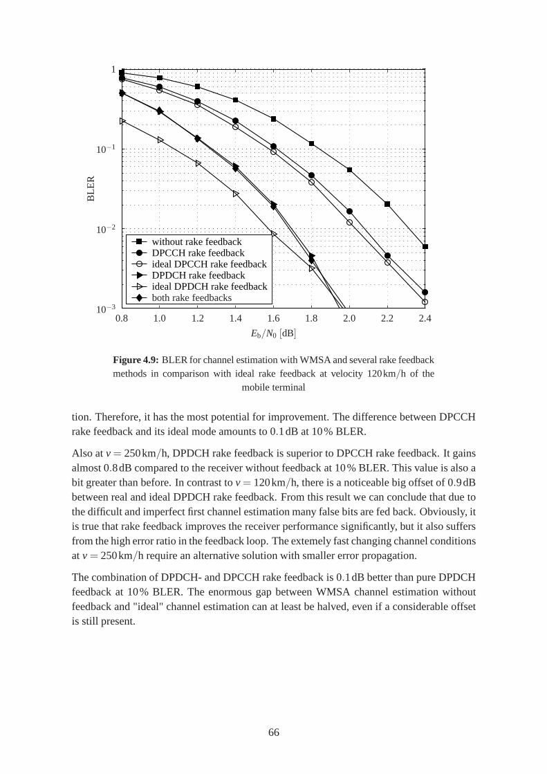
without rake feedbackDPCCH rake feedbackideal DPCCH rake feedbackDPDCH rake feedbackideal DPDCH rake feedbackboth rake feedback

0.8 1.0 1.2 1.4 1.6 1.8 2.0 2.2 2.4

Eb/N0 [dB]

10−3

10−2

10−1

1

BL

ER

both rake feedbacks

Figure 4.9: BLER for channel estimation with WMSA and several rake feedbackmethods in comparison with ideal rake feedback at velocity 120km/h of the

mobile terminal

tion. Therefore, it has the most potential for improvement.The difference between DPCCHrake feedback and its ideal mode amounts to 0.1dB at 10% BLER.

Also atv = 250km/h, DPDCH rake feedback is superior to DPCCH rake feedback. Itgainsalmost 0.8dB compared to the receiver without feedback at 10% BLER. This value is also abit greater than before. In contrast tov = 120km/h, there is a noticeable big offset of 0.9dBbetween real and ideal DPDCH rake feedback. From this resultwe can conclude that due tothe difficult and imperfect first channel estimation many false bits are fed back. Obviously, itis true that rake feedback improves the receiver performance significantly, but it also suffersfrom the high error ratio in the feedback loop. The extemely fast changing channel conditionsatv = 250km/h require an alternative solution with smaller error propagation.

The combination of DPDCH- and DPCCH rake feedback is 0.1dB better than pure DPDCHfeedback at 10% BLER. The enormous gap between WMSA channel estimation withoutfeedback and "ideal" channel estimation can at least be halved, even if a considerable offsetis still present.

66

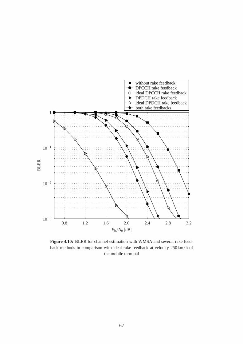
without rake feedbackDPCCH rake feedbackideal DPCCH rake feedbackDPDCH rake feedbackideal DPDCH rake feedbackboth rake feedbackboth rake feedbacks

0.8 1.2 1.6 2.0 2.4 2.8 3.2

Eb/N0 [dB]

10−3

10−2

10−1

1

BL

ER

Figure 4.10: BLER for channel estimation with WMSA and several rake feed-back methods in comparison with ideal rake feedback at velocity 250km/h of

the mobile terminal

67

Chapter 5

Channel estimation with decoderfeedback

5.1 The receiver with decoder feedback

In the previous chapter, a receiver with feedback loops after finger combining was discussedin detail. This rake feedback yields significant performance gains compared to the conven-tional receiver without feedback. However, the extended training sequence may exhibit ahigh bit error ratio due to an imperfect first channel estimation. The theoretically possibleperformance gain is not nearly achieved. This effect is mostclearly evident in Figure 4.10.Therefore, as an alternative solution, a receiver exploiting the error correcting property ofthe decoder and feeding back its output is presented in the following.

The design of the proposed receiver depends on the coding type. So far, all simulation resultswere obtained with a transmission system operating with turbo coding. Therefore, we firstlyturn to the decoder feedback design for turbo coding in Figure 5.1. Recapitulating Figure 2.6,the coded bit sequence consists of information bitsxk and parity bitszk andz′k. The parity bitsare output from a recursive shift register. Onlyxk are usable as extended training sequencebecause a wrong bit in the recursive shift register would cause error propagation, and animprovement of the channel estimates would not be possible.This comes along with thedisadvantage of a much smaller number of fed back bits compared to rake feedback. Inthe case exemplified in Appendix A, 3036 bits per TTI are available for decoder feedbackbecause only information bits of the evaluated transport channel (DTCH) are considered.Other transport channels may use a different coding scheme.In contrast, rake feedbackcan fall back on 9600 bits per TTI in total. Due to the shorter extended training sequenceΓD

κ,m, noise suppression on the channel estimates is not so effective as with rake feedback.Therefore, we have to expect a longer WMSA filter length and a worse channel trackingcompared to rake feedback.

After the channel estimator with outputh1,i and the MRC have been passed through once,finger combined samplesa1,i,m representing one TTI are input to the sample processor. The

69

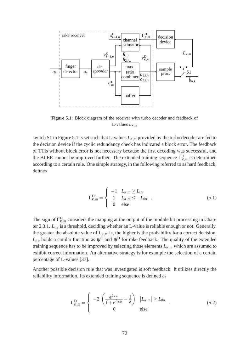
rake receiver

-qh

fingerdetector

-oc

de-spreader -

max.ratio

combiner-

a1,i,ma2,i,m

sampleproc.

?S1

-bν ,k

- buffer

rDi,m

rDκ,m

rCi+4,n

--

sCi+4,n

channelestimator

?

h1,ih2,i

Lκ,m

decisiondevice

ΓD

κ,m

Figure 5.1: Block diagram of the receiver with turbo decoder and feedback ofL-valuesLκ,m

switch S1 in Figure 5.1 is set such that L-valuesLκ,m provided by the turbo decoder are fed tothe decision device if the cyclic redundancy check has indicated a block error. The feedbackof TTIs without block error is not necessary because the firstdecoding was successful, andthe BLER cannot be improved further. The extended training sequenceΓD

κ,m is determinedaccording to a certain rule. One simple strategy, in the following referred to as hard feedback,defines

ΓDκ,m =

−1 Lκ,m ≥ Lthr

1 Lκ,m ≤−Lthr

0 else. (5.1)

The sign ofΓDκ,m considers the mapping at the output of the module bit processing in Chap-

ter 2.3.1.Lthr is a threshold, deciding whether an L-value is reliable enough or not. Generally,the greater the absolute value ofLκ,m is, the higher is the probability for a correct decision.Lthr holds a similar function asψC andψD for rake feedback. The quality of the extendedtraining sequence has to be improved by selecting those elementsLκ,m which are assumed toexhibit correct information. An alternative strategy is for example the selection of a certainpercentage of L-values [37].

Another possible decision rule that was investigated is soft feedback. It utilizes directly thereliability information. Its extended training sequence is defined as

ΓDκ,m =

−2

(

eLκ ,m

1+eLκ ,m− 1

2

)

∣

∣Lκ,m∣

∣≥ Lthr

0 else. (5.2)

70

The L-value definition from (2.40) is thereby considered. Besides the pure selection of L-values, a weighting related to the respectivea posterioriprobabilities is carried out. Hence,those elements which are more likely to exhibit correct information are weighted strongerthan others.

Now, updatesχ ′κ of the instantaneous channel estimatesχκ of all slotsκ of the fed back TTI

can be determined as

χ ′κ = ϒ

(

χκ +ζ D

NDF

Mκ∑

m=1

rDκ,m ΓD

κ,m

)

(5.3)

with the norming factorϒ from (4.8).ζ D is an arbitrary scaling factor controlling the portion

of ΓDκ,m in χ ′

κ . Mκ denotes the number of information bits of slotκ , andNDF =

∑Mκm=1

∣

∣

∣ΓD

κ,m

∣

∣

∣

is the effective length of the extended training sequence. The receiver with rake feedbackhas only updatesχ ′

κ of the present and past slotsκ = i −4, · · · , i at its disposal. In contrast,the receiver with decoder feedback can also fall back to the future slotsκ = i +1, · · · , i +4.As decoding is carried out as soon as one complete TTI was received, all L-values of thisTTI are available at the same time. This enables the calculation of all χ ′

κ in advance. Finally,the second WMSA channel estimation results in

h2,i =1

i+4∑

κ=i−4wD

κ

·

15J∑

κ=i−4wD

κ χκ +i+4∑

κ=1wD

κ χ ′κ i ≤ 4

i+4∑

κ=i−4wD

κ χ ′κ 5≤ i ≤ 15J−4

15J∑

κ=i−4wD

κ χ ′κ +

i+4∑

κ=1wD

κ χκ i ≥ 15J−3

. (5.4)

i = 1 indicates the first slot of a TTI andi = 15J the last one becauseJ is the number of framesper TTI, and one frame consists of 15 slots. The first case in (5.4) assumes the beginning ofthe channel observation time dating back to the previous TTIthat was possibly not fed back.Hence, updated valuesχ ′

κ are not available but only the buffered estimatesχκ . The thirdcase in (5.4) is also an exception handling. It is the other way round than before. The endof the channel observation time lies in the subsequent TTI. The delay between DPDCH andDPCCH ensures that the first four slots of the subsequent TTI were already processed in thechannel estimator, and theχκ are available. Generally, it is possible to establish a receiverthat avoids these exceptions. The first case is dropped if allTTIs are fed back, and not onlythose with a block error.χ ′

κ would then be available for all previous slots. An additionalartificial delay of one TTI in the feedback loop would preventthe third case because thenalso the subsequent TTI would be already decoded, and itsχ ′

κ would be available. However,decoder feedback was designed in particular for higher velocities of the mobile terminalexhibiting a short channel observation timeTobs. Therefore, the exception handling in (5.4)

71

is only of minor importance. As an example, forv= 250km/h they are decisive for only twoof sixty slots in total. The mentioned alternatives were notrealized, particularly since theycome along with some disadvantages, namely additional computation due to the feedback ofcorrect TTIs as well as an additional delay.

There is a time offset between first and second channel estimation. It cannot be found outuntil one complete TTI is decoded whether it contains a blockerror or not. The implemen-tation of decoder feedback therefore requires a buffer for received DPDCH samplesrD

i,m asshown in Figure 5.1. The instantaneous channel estimatesχi have also to be stored.

The second pass through the rake receiver is followed by a second chance to decode the fingercombined samplesa2,i,m without block errors. In principle, the feedback loop can bepassedthrough more than once in terms of an iterative information exchange between turbo decoderand channel estimator. The latter applies WMSA for each rakefinger individually, whereasthe turbo decoder processes a finger combined signal. An MRC connects both functions andprovides the input for the next decoding step. However, simulation results have shown thatthe BLER cannot be reduced considerably by that [38].

Finally, we switch S1 in Figure 5.1 such that the outputbν,k from the functional block sampleprocessing is available.

In the case that convolutional coding is applied, the sampleprocessing module contains aViterbi decoder providing the binary decided outputb1,ν,k after the first pass through therake receiver. A modification of the decoder feedback loop isrequired. Figure 5.2 shows therespective block diagram. In order to makeb1,ν,k applicable for a second channel estima-tion, the complete TTI has to be coded again. Therefore, the decision device in Figure 5.1is replaced by a bit processing module similar to that of the transmitter. Its output is theextended training sequenceΓD

κ,m. It consists of the re-encoded bits∈ ±1 of the transportchannelν under consideration (DTCH). The elements inΓD

κ,m belonging to other transportchannels are set to zero. Generally, also a receiver that exploits the complete re-encoded bitsequence is possible. As only TTIs with block errors are fed back,ΓD

κ,m includes bit errors.All bits exhibit the same error probability, and a further restriction of the extended trainingsequence in terms of a threshold decision is not possible. Asother transport channels are ex-cluded, the number of elements unequal zero inΓD

κ,m is smaller than for rake feedback withψD = 90. For the example in Appendix A it amounts to 4·2293= 9172 bits per TTI fordecoder feedback and 4·2400= 9600 for rake feedback. However, the number is increasedsignificantly compared to decoder feedback for turbo coding(3036 bits per TTI). Accordingto Figure 2.5, the mentioned disadvantage of recursive shift registers is not present for theused convolutional coding schemes.

The further processing in the feedback loop is the same as discussed before. The instanta-neous channel estimatesχκ are updated according to (5.3). (5.4) defines the second WMSAchannel estimation with the same exception handling. The TTI is decoded again after thesecond pass through the rake receiver. Finally, the binary outputb2,ν,k is available.

72

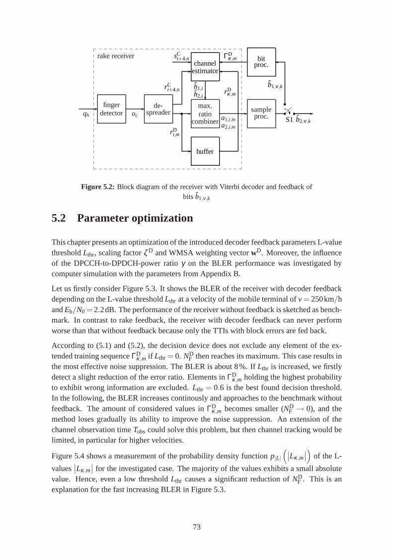
rake receiver

-qh

fingerdetector

-oc

de-spreader -

max.ratio

combiner-

a1,i,ma2,i,m

sampleproc.

-b2,ν ,k

- buffer

rDi,m

rDκ,m

rCi+4,n

--

sCi+4,n

channelestimator

?

h1,ih2,i

b1,ν ,k

bitproc.

ΓD

κ,m

?S1

Figure 5.2: Block diagram of the receiver with Viterbi decoder and feedback ofbits b1,ν ,k

5.2 Parameter optimization

This chapter presents an optimization of the introduced decoder feedback parameters L-valuethresholdLthr, scaling factorζ D and WMSA weighting vectorwD. Moreover, the influenceof the DPCCH-to-DPDCH-power ratioγ on the BLER performance was investigated bycomputer simulation with the parameters from Appendix B.

Let us firstly consider Figure 5.3. It shows the BLER of the receiver with decoder feedbackdepending on the L-value thresholdLthr at a velocity of the mobile terminal ofv= 250km/handEb/N0 = 2.2dB. The performance of the receiver without feedback is sketched as bench-mark. In contrast to rake feedback, the receiver with decoder feedback can never performworse than that without feedback because only the TTIs with block errors are fed back.

According to (5.1) and (5.2), the decision device does not exclude any element of the ex-tended training sequenceΓD

κ,m if Lthr = 0. NDF then reaches its maximum. This case results in

the most effective noise suppression. The BLER is about 8%. If Lthr is increased, we firstlydetect a slight reduction of the error ratio. Elements inΓD

κ,m holding the highest probabilityto exhibit wrong information are excluded.Lthr = 0.6 is the best found decision threshold.In the following, the BLER increases continously and approaches to the benchmark withoutfeedback. The amount of considered values inΓD

κ,m becomes smaller (NDF → 0), and the

method loses gradually its ability to improve the noise suppression. An extension of thechannel observation timeTobs could solve this problem, but then channel tracking would belimited, in particular for higher velocities.

Figure 5.4 shows a measurement of the probability density function p|L|(

∣

∣Lκ,m∣

∣

)

of the L-

values∣

∣Lκ,m∣

∣ for the investigated case. The majority of the values exhibits a small absolutevalue. Hence, even a low thresholdLthr causes a significant reduction ofND

F . This is anexplanation for the fast increasing BLER in Figure 5.3.

73

decoder feedback ondecoder feedback off

0 1 2 3 4 5 6 7L-value thresholdLthr

10−1

1

BL

ER

Figure 5.3: BLER of the receiver with decoder feedback at velocity 250km/hof the mobile terminal andEb/N0 = 2.2dB depending on the L-value threshold

Lthr

0 5 10 15 20∣

∣Lκ,m∣

∣

0.00

0.05

0.10

0.15

p |L|(

∣ ∣

Lκ,

m∣ ∣

)

Figure 5.4: Measured probability density functionp|L|(

∣

∣Lκ,m

∣

∣

)

of the L-values∣

∣Lκ,m∣

∣ at velocity 250km/h of the mobile terminal andEb/N0 = 2.2dB

74

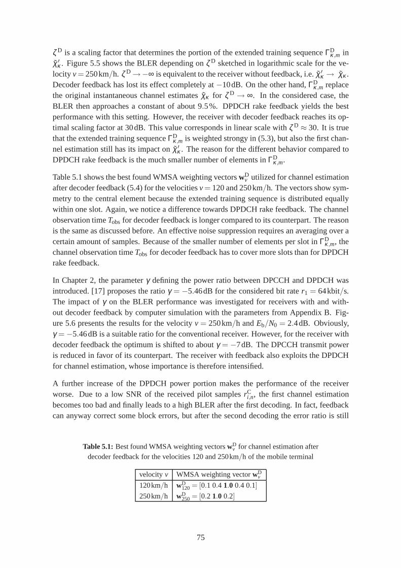
ζ D is a scaling factor that determines the portion of the extended training sequenceΓDκ,m in

χ ′κ . Figure 5.5 shows the BLER depending onζ D sketched in logarithmic scale for the ve-

locity v= 250km/h. ζ D →−∞ is equivalent to the receiver without feedback, i.e.χ ′κ → χκ .

Decoder feedback has lost its effect completely at−10dB. On the other hand,ΓDκ,m replace

the original instantaneous channel estimatesχκ for ζ D → ∞. In the considered case, theBLER then approaches a constant of about 9.5%. DPDCH rake feedback yields the bestperformance with this setting. However, the receiver with decoder feedback reaches its op-timal scaling factor at 30dB. This value corresponds in linear scale withζ D ≈ 30. It is truethat the extended training sequenceΓD

κ,m is weighted strongy in (5.3), but also the first chan-nel estimation still has its impact onχ ′

κ . The reason for the different behavior compared toDPDCH rake feedback is the much smaller number of elements inΓD

κ,m.

Table 5.1 shows the best found WMSA weighting vectorswDv utilized for channel estimation

after decoder feedback (5.4) for the velocitiesv= 120 and 250km/h. The vectors show sym-metry to the central element because the extended training sequence is distributed equallywithin one slot. Again, we notice a difference towards DPDCHrake feedback. The channelobservation timeTobs for decoder feedback is longer compared to its counterpart.The reasonis the same as discussed before. An effective noise suppression requires an averaging over acertain amount of samples. Because of the smaller number of elements per slot inΓD

κ,m, thechannel observation timeTobs for decoder feedback has to cover more slots than for DPDCHrake feedback.

In Chapter 2, the parameterγ defining the power ratio between DPCCH and DPDCH wasintroduced. [17] proposes the ratioγ = −5.46dB for the considered bit rater1 = 64kbit/s.The impact ofγ on the BLER performance was investigated for receivers withand with-out decoder feedback by computer simulation with the parameters from Appendix B. Fig-ure 5.6 presents the results for the velocityv = 250km/h andEb/N0 = 2.4dB. Obviously,γ = −5.46dB is a suitable ratio for the conventional receiver. However, for the receiver withdecoder feedback the optimum is shifted to aboutγ = −7dB. The DPCCH transmit poweris reduced in favor of its counterpart. The receiver with feedback also exploits the DPDCHfor channel estimation, whose importance is therefore intensified.

A further increase of the DPDCH power portion makes the performance of the receiverworse. Due to a low SNR of the received pilot samplesrC

i,n, the first channel estimationbecomes too bad and finally leads to a high BLER after the first decoding. In fact, feedbackcan anyway correct some block errors, but after the second decoding the error ratio is still

Table 5.1: Best found WMSA weighting vectorswDv for channel estimation after

decoder feedback for the velocities 120 and 250km/h of the mobile terminal

velocity v WMSA weighting vectorwDv

120km/h wD120 = [0.1 0.4 1.0 0.4 0.1]

250km/h wD250 = [0.2 1.0 0.2]

75

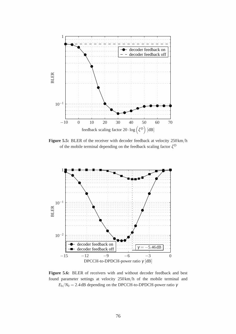
decoder feedback ondecoder feedback off

−10 0 10 20 30 40 50 60 70

feedback scaling factor 20· log(

ζ D)

[dB]

10−1

1

BL

ER

Figure 5.5: BLER of the receiver with decoder feedback at velocity 250km/hof the mobile terminal depending on the feedback scaling factor ζ D

decoder feedback ondecoder feedback off γ = −5.46dB

−15 −12 −9 −6 −3 0DPCCH-to-DPDCH-power ratioγ [dB]

10−2

10−1

1

BL

ER

Figure 5.6: BLER of receivers with and without decoder feedback and bestfound parameter settings at velocity 250km/h of the mobile terminal and

Eb/N0 = 2.4dB depending on the DPCCH-to-DPDCH-power ratioγ

76

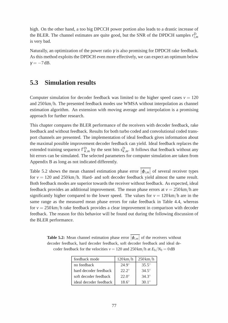
high. On the other hand, a too big DPCCH power portion also leads to a drastic increase ofthe BLER. The channel estimates are quite good, but the SNR ofthe DPDCH samplesrD

i,m

is very bad.

Naturally, an optimization of the power ratioγ is also promising for DPDCH rake feedback.As this method exploits the DPDCH even more effectively, we can expect an optimum belowγ = −7dB.

5.3 Simulation results

Computer simulation for decoder feedback was limited to thehigher speed casesv = 120and 250km/h. The presented feedback modes use WMSA without interpolation as channelestimation algorithm. An extension with moving average andinterpolation is a promisingapproach for further research.

This chapter compares the BLER performance of the receiverswith decoder feedback, rakefeedback and without feedback. Results for both turbo codedand convolutional coded trans-port channels are presented. The implementation of ideal feedback gives information aboutthe maximal possible improvement decoder feedback can yield. Ideal feedback replaces theextended training sequenceΓD

κ,m by the sent bitssDκ,m. It follows that feedback without any

bit errors can be simulated. The selected parameters for computer simulation are taken fromAppendix B as long as not indicated differently.

Table 5.2 shows the mean channel estimation phase error∣

∣ϕi,m∣

∣ of several receiver typesfor v = 120 and 250km/h. Hard- and soft decoder feedback yield almost the same result.Both feedback modes are superior towards the receiver without feedback. As expected, idealfeedback provides an additional improvement. The mean phase errors atv = 250km/h aresignificantly higher compared to the lower speed. The valuesfor v = 120km/h are in thesame range as the measured mean phase errors for rake feedback in Table 4.4, whereasfor v = 250km/h rake feedback provides a clear improvement in comparison with decoderfeedback. The reason for this behavior will be found out during the following discussion ofthe BLER performance.

Table 5.2: Mean channel estimation phase error∣

∣ϕi,m∣

∣ of the receivers withoutdecoder feedback, hard decoder feedback, soft decoder feedback and ideal de-

coder feedback for the velocitiesv = 120 and 250km/h atEb/N0 = 0dB

feedback mode 120km/h 250km/h

no feedback 24.9 35.5

hard decoder feedback 22.2 34.5

soft decoder feedback 22.0 34.3

ideal decoder feedback 18.6 30.1

77

Let us firstly discuss the speed casev = 120km/h in Figure 5.7. The presented receiversapply turbo decoding. In a first step, we only consider the curves which are labeled byγ = −5.46dB. Obviously, hard feedback and soft feedback perform almost equally. Softdecoder feedback yields only a small gain towards its counterpart at lowEb/N0. The curveswith feedback are steeper compared to that without feedback. The gain of the receivers withfeedback increases from 0.5dB at 10% BLER to 0.6dB at 1%. The offset between decoderfeedback and its ideal mode amounts to 0.35dB.

Considering the curve for hard decoder feedback with optimized power ratioγ = −7dB,we find a small additional gain of 0.1dB at 10% BLER compared to the default valueγ = −5.46dB proposed in [17]. This gain increases at higherEb/N0.

This statements are in principle also valid for the high speed casev = 250km/h. The asso-ciated BLER chart is shown in Figure 5.8. However, the gaps between the curves are largerthan before, which is due to the higher sensitivity of the receiver to variations of the parame-ters with increasing velocity. In detail, considering onlythe curves forγ =−5.46dB, we finda gain of the receiver with decoder feedback compared to thatwithout feedback of 0.6dB at10% BLER and even 0.7dB at 1%. The offset towards the ideal mode is about 0.65dB.

The optimization ofγ does not show the same impact as before. The gap between the curvesfor γ =−5.46dB andγ =−7dB is smaller than 0.1dB. Obviously, atv= 250km/h the per-formance of the receiver depends mainly on the channel estimation parameters, in particularthe channel observation timeTobs, and not so much on the DPCCH-to-DPDCH-power ratioγ. In the following, the evaluation is limited to the caseγ = −5.46dB.

A comparison of the best channel estimation method without feedback, the best rake feed-back mode and the best decoder feedback mode is also of big interest. According to Fig-ure 3.13, WMSA with interpolation is the most appropriate channel estimation method forthe velocity casev = 120km/h. In Figure 5.9, we find a gain of about 0.1dB at 10% BLERtowards WMSA channel estimation without interpolation. Obvioulsy, the feedback modesare superior to the receiver without feedback. Both rake anddecoder feedback are 0.4dBbetter than WMSA with interpolation and without feedback. The gaps between the curvesget larger with increasingEb/N0.

The advantage of decoder feedback is that its extended training sequenceΓDκ,m consists of

decoded and re-encoded values. It contains less bit errors compared to rake feedback. Onthe other hand, the length of the rake feedback extended training sequence is bigger thanits counterpart, namely 9600 compared to 3036 bits per TTI for the considered example.To achieve the same noise suppression, the channel observation timeTobs in rake feedbackmode can be reduced. This comes along with an improvement of the channel tracking.Furthermore, rake feedback enables the use of the non-pilotbits of the DPCCH for channelestimation. According to the presented results, the advantages of both designs are in balancefor the casev = 120km/h.

Applying the convolutional coder from Figure 2.5 with the same code ratec1 = 1/3, thelength ofΓD

κ,m is almost the same for rake- and for decoder feedback, namely9600 and 9172

78

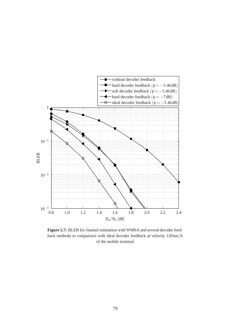
without decoder feedbackhard decoder feedback (γ = −5.46 dB)soft decoder feedback (γ = −5.46 dB)hard decoder feedback (γ = −7 dB)ideal decoder feedback (γ = −5.46 dB)

without decoder feedback

hard decoder feedback(γ = −5.46dB)

soft decoder feedback(γ = −5.46dB)

hard decoder feedback(γ = −7dB)

ideal decoder feedback(γ = −5.46dB)

0.8 1.0 1.2 1.4 1.6 1.8 2.0 2.2 2.4

Eb/N0 [dB]

10−3

10−2

10−1

1

BL

ER

Figure 5.7: BLER for channel estimation with WMSA and several decoder feed-back methods in comparison with ideal decoder feedback at velocity 120km/h

of the mobile terminal

79

without decoder feedbackhard decoder feedback (γ = −5.46 dB)soft decoder feedback (γ = −5.46 dB)hard decoder feedback (γ = −7 dB)ideal decoder feedback (γ = −5.46 dB)

without decoder feedback

hard decoder feedback(γ = −5.46dB)

soft decoder feedback(γ = −5.46dB)

hard decoder feedback(γ = −7dB)

ideal decoder feedback(γ = −5.46dB)

0.8 1.2 1.6 2.0 2.4 2.8 3.2

Eb/N0 [dB]

10−3

10−2

10−1

1

BL

ER

Figure 5.8: BLER for channel estimation with WMSA and several decoder feed-back methods in comparison with ideal decoder feedback at velocity 250km/h

of the mobile terminal

80

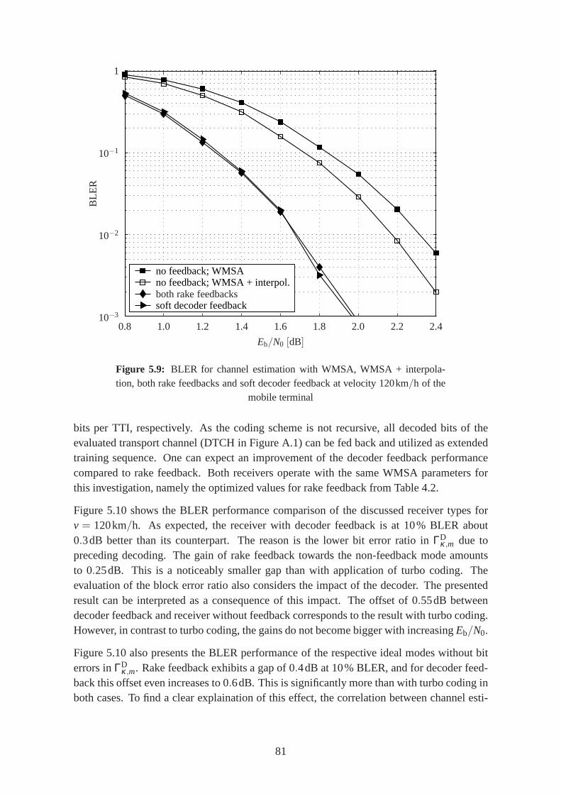
no feedback; WMSAno feedback; WMSA + interpol.both rake feedbacksoft decoder feedback

0.8 1.0 1.2 1.4 1.6 1.8 2.0 2.2 2.4

Eb/N0 [dB]

10−3

10−2

10−1

1

BL

ER

both rake feedbacks

Figure 5.9: BLER for channel estimation with WMSA, WMSA + interpola-tion, both rake feedbacks and soft decoder feedback at velocity 120km/h of the

mobile terminal

bits per TTI, respectively. As the coding scheme is not recursive, all decoded bits of theevaluated transport channel (DTCH in Figure A.1) can be fed back and utilized as extendedtraining sequence. One can expect an improvement of the decoder feedback performancecompared to rake feedback. Both receivers operate with the same WMSA parameters forthis investigation, namely the optimized values for rake feedback from Table 4.2.

Figure 5.10 shows the BLER performance comparison of the discussed receiver types forv = 120km/h. As expected, the receiver with decoder feedback is at 10% BLER about0.3dB better than its counterpart. The reason is the lower bit error ratio in ΓD

κ,m due topreceding decoding. The gain of rake feedback towards the non-feedback mode amountsto 0.25dB. This is a noticeably smaller gap than with applicationof turbo coding. Theevaluation of the block error ratio also considers the impact of the decoder. The presentedresult can be interpreted as a consequence of this impact. The offset of 0.55dB betweendecoder feedback and receiver without feedback corresponds to the result with turbo coding.However, in contrast to turbo coding, the gains do not becomebigger with increasingEb/N0.

Figure 5.10 also presents the BLER performance of the respective ideal modes without biterrors inΓD

κ,m. Rake feedback exhibits a gap of 0.4dB at 10% BLER, and for decoder feed-back this offset even increases to 0.6dB. This is significantly more than with turbo coding inboth cases. To find a clear explaination of this effect, the correlation between channel esti-

81

no feedback; WMSAboth rake feedbackideal rake feedbackdecoder feedbackideal decoder feedback

1.0 1.5 2.0 2.5 3.0 3.5 4.0

Eb/N0 [dB]

10−3

10−2

10−1

1

BL

ER

both rake feedbacks

Figure 5.10: BLER for several channel estimation methods of a transmissionsystem applying convolutional coding at velocity 120km/h of the mobile termi-

nal

mation, bit error ratio as well as error distribution beforedecoding and the respective codingscheme has to be investigated in more detail. Obviously, channel estimation with feedbackyields more improvement compared to the non-feedback mode if the receiver operates withturbo decoding. The good result of decoder feedback in connection with the Viterbi decoderis just a consequence of the increased length ofΓD

κ,m. However, in the case that optimalWMSA parameters depend on the coding scheme, one approach toimprove the performanceof a feedback receiver with Viterbi decoder is to look for better parameters for this specialcase.

Finally, a comparison of receivers with Turbo decoder for the high speedv = 250km/h ispresented in Figure 5.11. As illustrated in Figure 3.14, thebest channel estimation methodin the non-feedback mode is moving average with interpolation. Obviously, rake feedbackis superior to decoder feedback. At 10% BLER the difference amounts to about 0.2dB.The mentioned advantage of rake feedback predominates in this case. The reason is thatthe performance depends significantly on a short channel observartion time at very highspeed of the mobile terminal, and rake feedback allows for it. Furthermore, the gap betweenrake feedback and the receiver without feedback, which operates with moving average andinterpolation, is 0.4dB. A similar result was found forv = 120km/h. Finally, we find a gainof 0.9dB of rake feedback towards the receiver without feedback,which both use WMSAwithout interpolation.

82

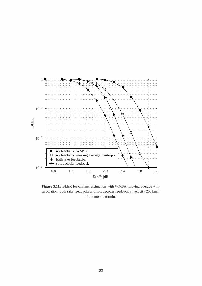
no feedback; WMSAno feedback; moving average + interpol.both rake feedbacksoft decoder feedback

0.8 1.2 1.6 2.0 2.4 2.8 3.2

Eb/N0 [dB]

10−3

10−2

10−1

1

BL

ER

both rake feedbacks

Figure 5.11: BLER for channel estimation with WMSA, moving average + in-terpolation, both rake feedbacks and soft decoder feedbackat velocity 250km/h

of the mobile terminal

83

Chapter 6

Velocity estimation

In Chapter 3, the channel estimation algorithms WMSA and moving average, both with op-tional interpolation, were presented and investigated forthe selected velocities of the mobileterminalv = 3,50,120 and 250km/h. It was found out that the performance of these fourmethods and the optimal channel observation timeTobs strongly depend onv. Thus, an ap-propriate channel estimation requires knowledge of the instantaneous velocity.

Firstly, an extended receiver is presented which estimatesthe speed of the mobile terminal byevaluating the power density spectrum of the compensated pilot samplesχn. Afterwards, theadaptation of the channel estimation parameters accordingto the estimated velocity ˆv is dis-cussed. The proposed method is compared with a conventionalreceiver without estimation.Finally, an alternative approach is sketched that operatesin the time domain.

6.1 Estimation in the frequency domain

The principle design of the proposed receiver is illustrated in Figure 6.1. Compared withthe well known receiver from Chapter 2.5, we find one additional functional blockvelocityestimatorthat provides one estimate ˆvi of the velocityv per sloti to the channel estimationmodule. As one input signal, pilot samplesrC

n are available. Of course,rCn represent only

one rake fingerl (l = 1, . . . ,L), but we drop the indexl for simplification. The followingderivation requires an assignment of the valuesrC

n to the corresponding sloti. Therefore, wewill use the notationrC

i,n. Remember that one DPCCH slot consists ofN = 10 samples. Thosewith indexn = 1, . . . ,NP are received pilots. Multiplication by the known pilot patternsC

i,n

yields the compensated pilot samplesχi,n = rCi,nsC

i,n. In order to obtain a continuous sequenceχi,n, we define the missing values with indexn = NP + 1, . . . ,10 by a linear interpolationbetweenχi,NP andχi+1,1 as

χi,NP+a = χi,NP +a · χi+1,1−χi,NP

11−NP, (6.1)

85

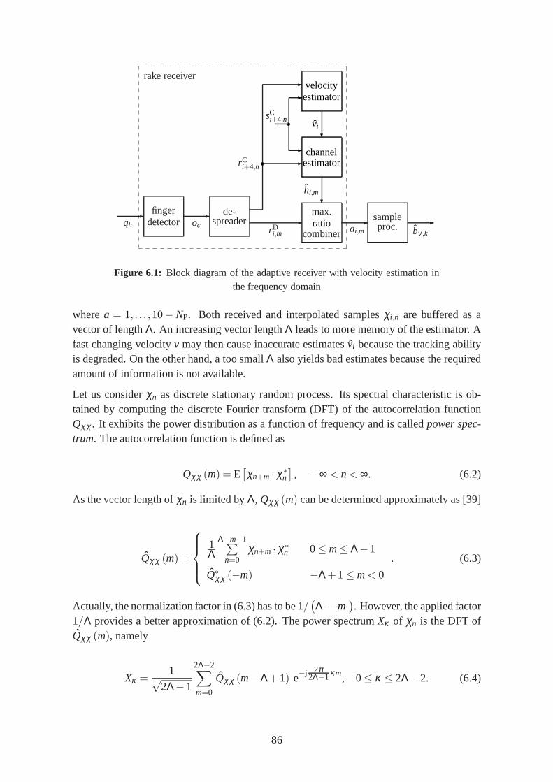
rake receiver

-qh

fingerdetector

-oc

de-spreader -

rDi,m

max.ratio

combiner-

ai,m

sampleproc.

-bν ,k

rCi+4,n

-

sCi+4,n

-

-

- velocityestimator

?vi

channelestimator

?hi,m

Figure 6.1: Block diagram of the adaptive receiver with velocity estimation inthe frequency domain

wherea = 1, . . . ,10− NP. Both received and interpolated samplesχi,n are buffered as avector of lengthΛ. An increasing vector lengthΛ leads to more memory of the estimator. Afast changing velocityv may then cause inaccurate estimates ˆvi because the tracking abilityis degraded. On the other hand, a too smallΛ also yields bad estimates because the requiredamount of information is not available.

Let us considerχn as discrete stationary random process. Its spectral characteristic is ob-tained by computing the discrete Fourier transform (DFT) ofthe autocorrelation functionQχχ . It exhibits the power distribution as a function of frequency and is calledpower spec-trum. The autocorrelation function is defined as

Qχχ (m) = E[

χn+m ·χ∗n

]

, −∞ < n < ∞. (6.2)

As the vector length ofχn is limited byΛ, Qχχ (m) can be determined approximately as [39]

Qχχ (m) =

1Λ

Λ−m−1∑

n=0χn+m ·χ∗

n 0≤ m≤ Λ−1

Q∗χχ (−m) −Λ+1≤ m< 0

. (6.3)

Actually, the normalization factor in (6.3) has to be 1/(

Λ−|m|)

. However, the applied factor1/Λ provides a better approximation of (6.2). The power spectrum Xκ of χn is the DFT ofQχχ (m), namely

Xκ =1√

2Λ−1

2Λ−2∑

m=0

Qχχ (m−Λ+1) e−j 2π2Λ−1κm, 0≤ κ ≤ 2Λ−2. (6.4)

86

As Qχχ (m) exhibits conjugate symmetry,Xκ is real.

According to (3.3), it isχn = h′n in the noise-free case. Thus,Xκ shows the spectral char-acteristic of a multipath tap. As discussed in Chapter 2.4, the power spectrum ofh′n isdistributed between− fD,max and+ fD,max. Two measurements ofXκ are presented in Fig-ure 6.2. The velocity of the mobile terminal was set tov = 120km/h, which leads to themaximal Doppler frequencyfD,max≈ 222Hz. The indexκ allows for the derivation of thecorresponding Doppler frequencyfDκ . The left diagram shows the noise-free case, and theright one illustrates an example withEb/N0 = 0dB. The used channel model assumes aJakes distribution of the Doppler power density spectrum ofthe fading sequenceh(t) [16].Its characteristic shape is clearly visible in both measurements ofXκ . The maximal DopplerfrequencyfD,max can be estimated easily as

fD,maxi =∣

∣

∣fDargmax(Xκ )

∣

∣

∣. (6.5)

This estimation is executed once per slot afterXκ was updated. Differently shaped powerspectraXκ require more sophisticated detection algorithms. Some channel models assumemultipath taps with Gaussian distributed Doppler power density spectra, e.g. [40]. Knowl-edge of fD,maxi enables the calculation of the instantaneous velocity estimatev′i = fD,maxi ·c/ f0.

The determination of the velocity estimate ˆvi also considers the previous value ˆvi−1 as aconsequence of possible detection errors offD,max due to noise and statistical variations, i.e.

vi =η · vi−1+ v′i

η +1. (6.6)

The weighting factorη controls how strong the previous value ˆvi−1 is considered comparedto the instantaneous estimate ˆv′i .

6.2 Velocity classes and parameter optimization

The aim of velocity estimation is an adaptation of the channel estimation parameters. Op-timized parameters are only known for the velocitiesv = 3,50,120 and 250km/h. Theseparameters were used for various other velocities in between in order to find out borders ofso-called velocity classes. Within one velocity class the same estimation method and thesame WMSA weighting vectorw or moving average target filter lengthΩ are used. An al-ternative solution is an individual optimization for velocities in a certain grid. This wouldrequire an extreme expenditure. Another approach is an interpolation of the elements ofw or of Ω, respectively. Both alternatives may yield a further improvement of the receiverperformance.

87

−300 0 300Doppler frequencyfDκ [Hz]

0

2

4

6 ×10−5po

wer

spec

trum

Xκ

(a)

−300 0 300Doppler frequencyfDκ [Hz]

0

2

4

6 ×10−5

pow

ersp

ectr

umX

κ

(b)

Figure 6.2: Measured power spectraXκ of χn (a) in the noise-free case and (b)atEb/N0 = 0dB

For v = 50km/h, WMSA without interpolation is the best channel estimation method, andw50 = [1 1 1 11 1 1 1 1] is the optimal WMSA weighting vector. As the same was found outfor the low speedv= 3km/h, it is assumed that these settings of the receiver are also appro-priate for the velocities in between. However, forv = 120km/h WMSA with interpolationandw120 = [0.1 0.6 1.0 0.9 0.3] define the best estimator. The four possible combinationsof these settings were tested for 50km/h≤ v≤ 120km/h. The result in terms of BLER ispresented in Figure 6.3. The parameters from Appendix B wereused for computer simula-tion. Obviously, the combination WMSA with interpolation and w50 is the best choice forvelocities aroundv = 65km/h. To simplify matters, we restrict to two velocity classes withthe borderv = 65km/h.

Figure 6.4 shows a similar investigation for the velocity range from 120 to 250km/h. For thevery high speed, moving average with interpolation is the best channel estimation method,andΩ250 = 11 is the optimal target filter length. Again, the four possible combinations ofmethod and respective optimized parameter were tested. Obviously, we have to distinguishthree velocity cases:v< 140km/h requires WMSA with interpolation and weighting vectorw120. WMSA with interpolation and weighting vectorw250 = [0.0 1.0 0.3] are the appropri-ate channel estimation settings for 140km/h≤ v < 220km/h. Finally, for velocities higherthan 220km/h moving average with interpolation and target filter lengthΩ250 = 11 yieldthe best result. Table 6.1 summarizes the four found velocity classes and their respectiveparameter settings.

The parametersΛ andη determine the accuracy of the velocity estimates. For theiropti-mization a fading sequenceh(t) was generated that implies a certain velocity profile. Toemphasize this time-variance, we will denote the actual velocity with the additional slot in-

88

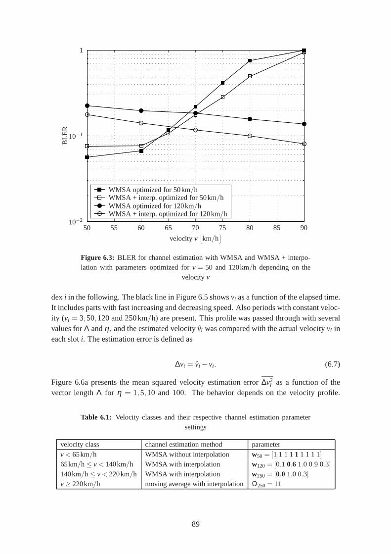
WMSA optimized for 50 km/hWMSA + interp. optimized for 50 km/hWMSA optimized for 120 km/hWMSA + interp. optimized for 120 km/h

50 55 60 65 70 75 80 85 90

velocity v[

km/h]

10−2

10−1

1

BL

ER

WMSA optimized for 50km/hWMSA + interp. optimized for 50km/hWMSA optimized for 120km/hWMSA + interp. optimized for 120km/h

Figure 6.3: BLER for channel estimation with WMSA and WMSA + interpo-lation with parameters optimized forv = 50 and 120km/h depending on the

velocity v

dexi in the following. The black line in Figure 6.5 showsvi as a function of the elapsed time.It includes parts with fast increasing and decreasing speed. Also periods with constant veloc-ity (vi = 3,50,120 and 250km/h) are present. This profile was passed through with severalvalues forΛ andη, and the estimated velocity ˆvi was compared with the actual velocityvi ineach sloti. The estimation error is defined as

∆vi = vi −vi . (6.7)

Figure 6.6a presents the mean squared velocity estimation error ∆v2i as a function of the

vector lengthΛ for η = 1,5,10 and 100. The behavior depends on the velocity profile.

Table 6.1: Velocity classes and their respective channel estimation parametersettings

velocity class channel estimation method parameter

v < 65km/h WMSA without interpolation w50 = [1 1 1 11 1 1 1 1]65km/h≤ v < 140km/h WMSA with interpolation w120 = [0.1 0.6 1.0 0.9 0.3]

140km/h≤ v < 220km/h WMSA with interpolation w250 = [0.0 1.0 0.3]

v≥ 220km/h moving average with interpolation Ω250 = 11

89

WMSA + interpolation optimized for 120 km/hmoving average + interp. optimized for 120 km/hWMSA + interpolation optimized for 250 km/hmoving average + interp. optimized for 250 km/h

120 140 160 180 200 220 240

velocity v[

km/h]

10−2

10−1

1

BL

ER

WMSA + interpolation optimized for 120km/hmoving average + interp. optimized for 120km/hWMSA + interpolation optimized for 250km/hmoving average + interp. optimized for 250km/h

Figure 6.4: BLER for channel estimation with WMSA + interpolation and mov-ing average + interpolation with parameters optimized forv= 120 and 250km/h

depending on the velocityv

Another scenario may lead to different results. Obviously,the estimates ˆvi become betterwith increasing weighting factorη. Among the investigated values,η = 100 yields the bestperformance. A largeη mitigates the influence of outliers of the instantaneous estimatesv′i on vi . This is advantageous for constant or slowly changing speed. However, trackinga fast changing velocity requires a lowerη. The curve forη = 1 reaches its minimumat Λ = 5000, whereas forη = 100 the smaller vector lengthΛ = 3000 provides the bestestimates. Generally,Λ has a similar effect on ˆvi asη. A large value buffers more pilotsamples and thus comes along with more memory. Both very small and very big vectorlengthsΛ cause a significant increase of the estimation error. In the first case, the smallamount of available information leads to rather inaccurateestimates and statistical variations.If the estimator operates with a too big vector length, it cannot adapt fast enough to thechanging speed and therefore provides bad estimates.

However, a velocity estimation error does not influence the block error ratio as long asvi

and vi belong to the same velocity class. A further evaluation has determined the velocityclass estimation error ratio. It is defined as the ratio between the number of estimates ˆvi ,which belong to a different velocity class thanvi , and the total number of estimates. Theresult is presented in Figure 6.6b. Now, estimators with smaller weighting factorsη yieldbetter results. The reason is a better tracking behavior during the periods with continuously

90

actual velocity vi

estimated velocity vi

actual velocityvi

estimated velocity ˆvi

150

125

10035 37.5 40

300

250

200

150

100

50

0

velocity[km

/h]

0 10 20 30 40 50 60time [s]

Figure

6.5:V

elocityv

iand

estimated

velocityˆ

vi

obtainedw

ithvector

lengthΛ

=3000

andw

eightingfactor η

=10

asfunctions

oftime

91

η = 1η = 10η = 50η = 100

2000 4000 6000 8000 10000

vector lengthΛ

10

14

18

22

26

30

mea

nsq

uare

dve

loci

tyes

timat

ion

erro

r∆v

2 i

(a)

η = 1η = 10η = 50η = 100

η = 1η = 10η = 50η = 100

2000 4000 6000 8000 10000

vector lengthΛ

1.5

2.0

2.5

3.0

3.5

4.0

4.5

velo

city

clas

ses

timat

ion

erro

rra

tio[%]

(b)

η = 1η = 10η = 50η = 100

Figure 6.6: (a) Mean squared velocity estimation error∆v2i and (b) velocity class

estimation error ratio depending on the vector lengthΛ and the weighting factorη

92

increasing or decreasing speed. On the other hand, bigger variations of vi during periodswith constant velocityvi have almost no influence on the velocity class estimation error ratiobecause the constant velocities have a large offset towardsthe velocity class borders in theconsidered case. If the velocityvi would be kept constant near to such a border, we wouldobtain a rather different result. Therefore, a general parameter optimization is difficult.

Λ = 3000 yields the smallest velocity class estimation error ratio for all considered weightingfactorsη. With η = 10 we obtain 1.85% as the smallest overall error ratio. Therefore, thevelocity estimator operates withΛ = 3000 andη = 10 for the following investigations.

The gray curve in Figure 6.5 shows the course of the estimatesvi as a function of time.The drops are the consequence of outliers. In this cases, a smaller frequency was wronglydetected as the maximal Doppler frequencyfD,max. In particular low and medium speedsbetween 50 and 120km/h seem susceptible to this weak point. One possible reason maybe the used fading sequenceh(t). Outliers to higher Doppler frequencies do not occur.The estimated velocity ˆvi is always equal to or smaller than the actual velocityvi . Duringthe period with constant high speedvi = 250km/h, the estimation works excellently. Asparticularly for higher velocities an accurate setting of the channel estimation parameters isabsolutely necessary, this knowledge is promising for a receiver that operates with adaptivechannel estimation.

6.3 Adaptive channel estimation

A receiver with adaptive channel estimator selects its parameters, namely algorithm andWMSA weighting vectorw or moving average target filter lengthΩ, respectively, accordingto the estimated velocity class. The velocity estimator utilizes optimized parametersΛ andη. This receiver is compared to its non-adaptive counterpartoperating with WMSA and theconstant weighting vectorw = [1 1 1], which is a fair compromise between the demands forboth low and high speed. For computer simulation, the velocity profile in Figure 6.5 waspassed through once. The other parameters are listed in Appendix B.

The result in terms of block error ratio is presented in Figure 6.7. Both receivers are addi-tionally compared to that operating with "ideal" channel estimation. The block errors are notdistributed equally over the simulated velocity profile. According to the respective speedvi ,the setEb/N0 is either high enough to avoid block errors or too bad, thus causing a lot ofwrong blocks. Figure 6.7 shows the overall result. It is the superposition of several effects.Obviously, the chart can be divided into two parts. The first one ranges fromEb/N0 = 0dBto about 4dB. The receiver with adaptive channel estimator yields a significant improvementof partially more than 1dB towards the conventional receiver. The reason is that the blockerrors occur mainly during the period with high speed. We have found out in previous chap-ters that the performance of the receiver is very sensitive to non-optimal channel estimationparameters at high speed. Therefore, the adaptive channel estimator can exploit its advantageeffectively and reduce the error ratio.

93

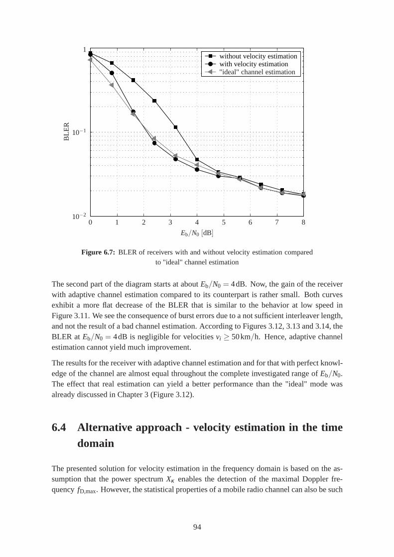
without velocity estimationwith velocity estimationideal channel estimation

0 1 2 3 4 5 6 7 8

Eb/N0 [dB]

10−2

10−1

1

BL

ER

"ideal" channel estimation

Figure 6.7: BLER of receivers with and without velocity estimation comparedto "ideal" channel estimation

The second part of the diagram starts at aboutEb/N0 = 4dB. Now, the gain of the receiverwith adaptive channel estimation compared to its counterpart is rather small. Both curvesexhibit a more flat decrease of the BLER that is similar to the behavior at low speed inFigure 3.11. We see the consequence of burst errors due to a not sufficient interleaver length,and not the result of a bad channel estimation. According to Figures 3.12, 3.13 and 3.14, theBLER at Eb/N0 = 4dB is negligible for velocitiesvi ≥ 50km/h. Hence, adaptive channelestimation cannot yield much improvement.

The results for the receiver with adaptive channel estimation and for that with perfect knowl-edge of the channel are almost equal throughout the completeinvestigated range ofEb/N0.The effect that real estimation can yield a better performance than the "ideal" mode wasalready discussed in Chapter 3 (Figure 3.12).

6.4 Alternative approach - velocity estimation in the timedomain

The presented solution for velocity estimation in the frequency domain is based on the as-sumption that the power spectrumXκ enables the detection of the maximal Doppler fre-quencyfD,max. However, the statistical properties of a mobile radio channel can also be such

94

that the detection is inaccurate or even fails. Therefore, an alternative approach is proposed,namely estimation in the time domain [41].

Figure 6.8 shows the design of this receiver. The WMSA channel estimatehi is input tothe velocity estimator. The basic idea is the observation ofhi in the complex plane over thetime. Generally, the time variation ofhi is related to the velocityvi of the mobile subscriber.

One possible solution is to measure the phase rotation∆φi =∣

∣

∣arc

hi−1

− arc

hi

∣

∣

∣. A

general approach defines the velocity estimate ˆvi as a function of the expectation of∆φi .Measurements have shown that E

[

∆φi]

depends on the actual velocityvi and the signal-to-noise ratioEb/N0. E

[

∆φi]

increases with higher velocityvi and with higher noise power [41].

The velocity estimate ˆvi controls the channel estimation parameters in the same way as be-fore. However, due to the feedback an adaptation is only possible for the subsequent sloti +1. The main disadvantage of the proposed method is the possibility of error propagation.Bad channel estimates can lead to bad velocity estimates andthe other way round. The re-ceiver can become instable. Therefore, the receiver in Figure 6.1 operating in the frequencydomain is the preferable solution.

rake receiver

-qh

fingerdetector

-oc

de-spreader -

rDi,m

max.ratio

combiner-

ai,m

sampleproc.

-bν ,k

rCi+4,n

--

sCi+4,n

channelestimator

?

hi- velocity

estimator

vi

?

Figure 6.8: Block diagram of the adaptive receiver with velocity estimation inthe time domain

95

Chapter 7

Conclusion

The work at hand presents a detailed model of an uplink transmissions system based on thephysical layer air interfaceUu of the third generation mobile radio system UMTS. One keyfunction of the receiver is channel estimation. After the finger detector has separated the re-ceived signal components originating from several propagation paths, the channel estimatorprovides estimates of the complex fading channel coefficients for each finger individually.Hence it follows that the fingers can be combined coherently,and the resulting signal isfinally input to the decoder for further processing.

In Chapter 3, several algorithms for estimating the channelcoefficients without any feedbackof a finger combined signal were presented. Firstly,weighted multi-slot averaging(WMSA)was investigated in detail. It was found out that the optimalchannel observation time stronglydepends on the velocity of the mobile terminal. Fast moving terminals do not allow a longobservation time because otherwise the channel estimator cannot track the fast changingchannel conditions. On the other hand, the estimates sufferfrom noise. Due to averaging ofreceived pilot samples, the impact of noise can be reduced. As a rule of thumb, the channelobservation time has to be as long as the variation of the channel coefficients allows for.Optimized WMSA weighting vectors were determined for selected velocities.

As WMSA provides only one channel estimate per slot, the alternative solutionmoving av-eragewas presented. This algorithm can be seen as generalizationof WMSA. It enables anindividual weighting of each single pilot sample. Therefore, one estimate per DPCCH bitinterval is available. Also for moving average, the parameter that controls the channel obser-vation time was optimized for several velocities. Both WMSAand moving average can bemodified by an additional interpolation between the available estimates. Finally, these fourcombinations were compared in terms of bit error ratio afterdecoding and block error ratio.It was found out that moving average and interpolation are only superior to WMSA at highervelocities of the mobile terminal.

A method exploiting also the non-pilot portion of the received signal was studied in Chap-ter 4. One can distinguish three possible cases: Feedback ofthe finger combined DPCCHnon-pilot samples to the channel estimator, feedback of theDPDCH samples and the con-catenation of both loops. As the feedback is applied within the rake receiver, this approach

97

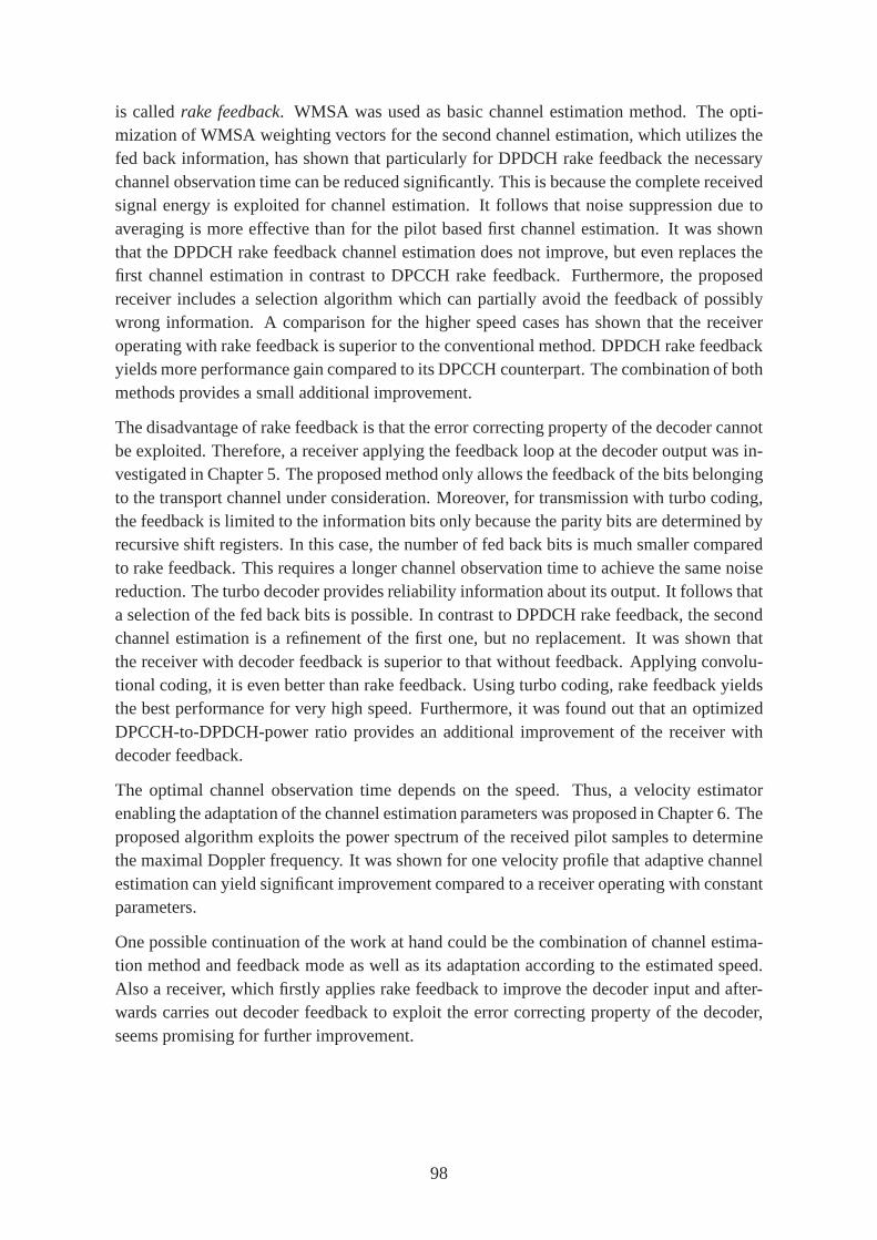
is calledrake feedback. WMSA was used as basic channel estimation method. The opti-mization of WMSA weighting vectors for the second channel estimation, which utilizes thefed back information, has shown that particularly for DPDCHrake feedback the necessarychannel observation time can be reduced significantly. Thisis because the complete receivedsignal energy is exploited for channel estimation. It follows that noise suppression due toaveraging is more effective than for the pilot based first channel estimation. It was shownthat the DPDCH rake feedback channel estimation does not improve, but even replaces thefirst channel estimation in contrast to DPCCH rake feedback.Furthermore, the proposedreceiver includes a selection algorithm which can partially avoid the feedback of possiblywrong information. A comparison for the higher speed cases has shown that the receiveroperating with rake feedback is superior to the conventional method. DPDCH rake feedbackyields more performance gain compared to its DPCCH counterpart. The combination of bothmethods provides a small additional improvement.

The disadvantage of rake feedback is that the error correcting property of the decoder cannotbe exploited. Therefore, a receiver applying the feedback loop at the decoder output was in-vestigated in Chapter 5. The proposed method only allows thefeedback of the bits belongingto the transport channel under consideration. Moreover, for transmission with turbo coding,the feedback is limited to the information bits only becausethe parity bits are determined byrecursive shift registers. In this case, the number of fed back bits is much smaller comparedto rake feedback. This requires a longer channel observation time to achieve the same noisereduction. The turbo decoder provides reliability information about its output. It follows thata selection of the fed back bits is possible. In contrast to DPDCH rake feedback, the secondchannel estimation is a refinement of the first one, but no replacement. It was shown thatthe receiver with decoder feedback is superior to that without feedback. Applying convolu-tional coding, it is even better than rake feedback. Using turbo coding, rake feedback yieldsthe best performance for very high speed. Furthermore, it was found out that an optimizedDPCCH-to-DPDCH-power ratio provides an additional improvement of the receiver withdecoder feedback.

The optimal channel observation time depends on the speed. Thus, a velocity estimatorenabling the adaptation of the channel estimation parameters was proposed in Chapter 6. Theproposed algorithm exploits the power spectrum of the received pilot samples to determinethe maximal Doppler frequency. It was shown for one velocityprofile that adaptive channelestimation can yield significant improvement compared to a receiver operating with constantparameters.

One possible continuation of the work at hand could be the combination of channel estima-tion method and feedback mode as well as its adaptation according to the estimated speed.Also a receiver, which firstly applies rake feedback to improve the decoder input and after-wards carries out decoder feedback to exploit the error correcting property of the decoder,seems promising for further improvement.

98

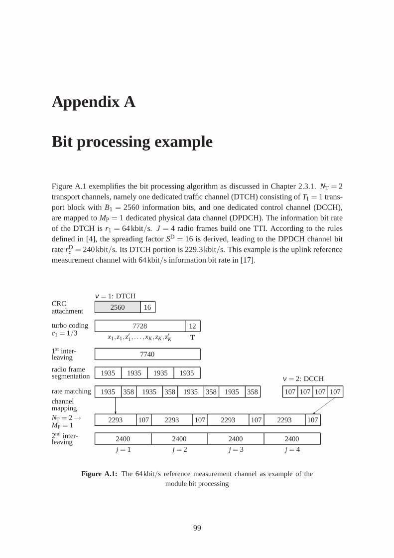
Appendix A

Bit processing example

Figure A.1 exemplifies the bit processing algorithm as discussed in Chapter 2.3.1.NT = 2transport channels, namely one dedicated traffic channel (DTCH) consisting ofT1 = 1 trans-port block withB1 = 2560 information bits, and one dedicated control channel (DCCH),are mapped toMP = 1 dedicated physical data channel (DPDCH). The informationbit rateof the DTCH isr1 = 64kbit/s. J = 4 radio frames build one TTI. According to the rulesdefined in [4], the spreading factorSD = 16 is derived, leading to the DPDCH channel bitraterD

c = 240kbit/s. Its DTCH portion is 229.3kbit/s. This example is the uplink referencemeasurement channel with 64kbit/s information bit rate in [17].

CRCattachment

turbo codingc1 = 1/3

1st inter-leaving

radio framesegmentation

rate matching

channelmappingNT = 2→MP = 1

2nd inter-leaving

ν = 1: DTCH

2560 16

7728

x1,z1,z′1, . . . ,xK ,zK ,z′K

12

T

7740

1935 1935 1935 1935

1935 358 1935 358 1935 358 1935 358

ν = 2: DCCH

107 107 107 107

? =2293 107 2293 107 2293 107 2293 107

2400 2400 2400 2400

j = 1 j = 2 j = 3 j = 4

Figure A.1: The 64kbit/s reference measurement channel as example of themodule bit processing

99

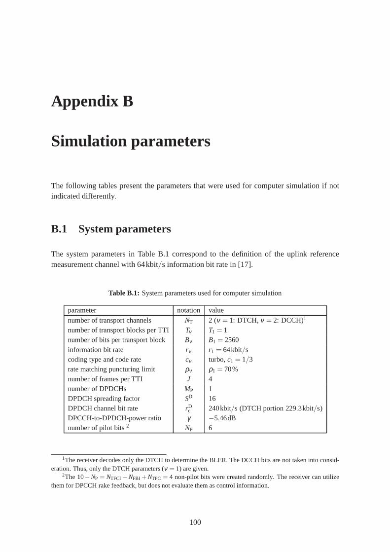
Appendix B

Simulation parameters

The following tables present the parameters that were used for computer simulation if notindicated differently.

B.1 System parameters

The system parameters in Table B.1 correspond to the definition of the uplink referencemeasurement channel with 64kbit/s information bit rate in [17].

Table B.1: System parameters used for computer simulation

parameter notation value

number of transport channels NT 2 (ν = 1: DTCH,ν = 2: DCCH)1

number of transport blocks per TTI Tν T1 = 1number of bits per transport block Bν B1 = 2560information bit rate rν r1 = 64kbit/scoding type and code rate cν turbo,c1 = 1/3rate matching puncturing limit ρν ρ1 = 70%number of frames per TTI J 4number of DPDCHs MP 1DPDCH spreading factor SD 16DPDCH channel bit rate rD

c 240kbit/s (DTCH portion 229.3kbit/s)DPCCH-to-DPDCH-power ratio γ −5.46dBnumber of pilot bits2 NP 6

1The receiver decodes only the DTCH to determine the BLER. TheDCCH bits are not taken into consid-eration. Thus, only the DTCH parameters (ν = 1) are given.

2The 10−NP = NTFCI + NFBI + NTPC = 4 non-pilot bits were created randomly. The receiver can utilizethem for DPCCH rake feedback, but does not evaluate them as control information.

100

B.2 Mobile radio channel parameters

The mobile radio channel parameters in Table B.2 correspondwith velocityv= 120km/h ofthe mobile terminal to the multipath fading propagation conditionsCase 3defined in [17],and withv = 250km/h to Case 4, respectively. All multipath taps exhibit classical Dopplerspectrum [16].

Table B.2: Mobile radio channel parameters used for computer simulation

parameter notation value

number of multipath taps Z 4mean relative attenuation1 dz d1 = 0dB,d2 = 3dB,d3 = 6dB,d4 = 9dBrelative path delay2 τz τ1 = 0ns,τ2 = 260ns,τ3 = 521ns,τ4 = 781ns

B.3 Receiver parameters

Table B.3: General receiver parameters used for computer simulation

parameter notation value

number of receive antennas A 2number of rake fingers3 L 8number of turbo decoder iterations IT 4WMSA weighting vector for the first CE wv w3 = [1 1 1 11 1 1 1 1]

w50 = [1 1 1 11 1 1 1 1]w120 = [0.1 0.6 1.0 0.9 0.3]

w250 = [1.0 0.3]

moving average target filter length Ωv Ω3 = 54,Ω50 = 51,Ω120 = 24,Ω250 = 11

1Due to an additional scaling the channel in total has no attenuation, i.e. E[

∣

∣u(t)∣

∣

]

= E[

∣

∣y(t)∣

∣

]

.2The delays are shifted onto the used oversampling grid givenby MOS = 4.3As ideal finger detection is assumed, all fingers are always present andL = A ·Z.

101

Table B.4: Receiver parameters used for computer simulation of rake feedback

parameter notation value

WMSA weighting vector for DPCCH rake feedback wCv wC

120 = [0.4 0.8 1.0 0.8 0.4]

wC250 = [0.2 1.0 0.2]

feedback threshold angle for DPCCH rake feedback ψC 80

feedback scaling factor for DPCCH rake feedback ζ C 0dB

WMSA weighting vector for DPDCH rake feedback wDv wD

120 = [0.1 1.0 0.1]

wD250 = [1.0]

feedback threshold angle for DPDCH rake feedback ψD 85

feedback scaling factor for DPDCH rake feedback ζ D 80dB

Table B.5: Receiver parameters used for computer simulation of decoder feed-back

parameter notation value

WMSA weighting vector for decoder feedback wDv wD

120 = [0.1 0.4 1.0 0.4 0.1]

wD250 = [0.2 1.0 0.2]

L-value threshold Lthr 0.6feedback scaling factor for DPCCH rake feedback ζ D 30dB

Table B.6: Receiver parameters used for computer simulation of velocity esti-mation

parameter notation value

number of collected and interpolated valuesχn Λ 3000weighting factor η 10

102

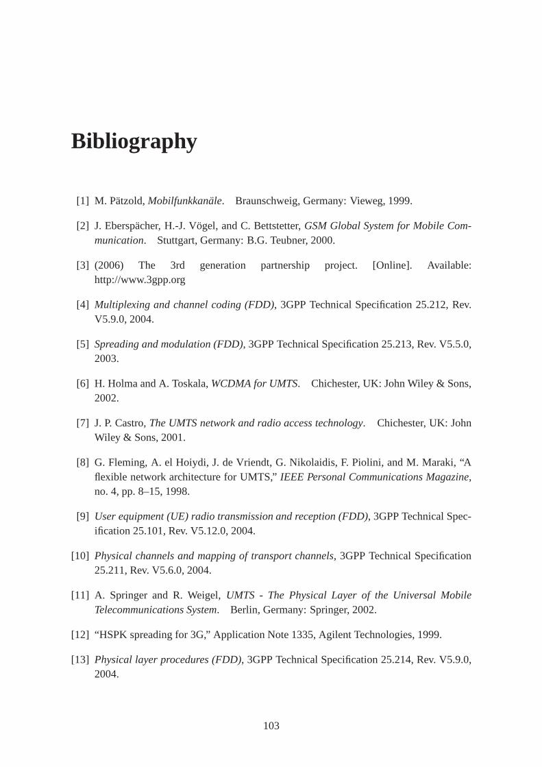
Bibliography

[1] M. Pätzold,Mobilfunkkanäle. Braunschweig, Germany: Vieweg, 1999.

[2] J. Eberspächer, H.-J. Vögel, and C. Bettstetter,GSM Global System for Mobile Com-munication. Stuttgart, Germany: B.G. Teubner, 2000.

[3] (2006) The 3rd generation partnership project. [Online]. Available:http://www.3gpp.org

[4] Multiplexing and channel coding (FDD), 3GPP Technical Specification 25.212, Rev.V5.9.0, 2004.

[5] Spreading and modulation (FDD), 3GPP Technical Specification 25.213, Rev. V5.5.0,2003.

[6] H. Holma and A. Toskala,WCDMA for UMTS. Chichester, UK: John Wiley & Sons,2002.

[7] J. P. Castro,The UMTS network and radio access technology. Chichester, UK: JohnWiley & Sons, 2001.

[8] G. Fleming, A. el Hoiydi, J. de Vriendt, G. Nikolaidis, F.Piolini, and M. Maraki, “Aflexible network architecture for UMTS,”IEEE Personal Communications Magazine,no. 4, pp. 8–15, 1998.

[9] User equipment (UE) radio transmission and reception (FDD), 3GPP Technical Spec-ification 25.101, Rev. V5.12.0, 2004.

[10] Physical channels and mapping of transport channels, 3GPP Technical Specification25.211, Rev. V5.6.0, 2004.

[11] A. Springer and R. Weigel,UMTS - The Physical Layer of the Universal MobileTelecommunications System. Berlin, Germany: Springer, 2002.

[12] “HSPK spreading for 3G,” Application Note 1335, Agilent Technologies, 1999.

[13] Physical layer procedures (FDD), 3GPP Technical Specification 25.214, Rev. V5.9.0,2004.

103

[14] B. Sklar, “Rayleigh fading channels in mobile digital communication systems Part I:Characterization,”IEEE Communications Magazine, vol. 35, no. 9, pp. 136–146, 1997.

[15] P. Hoeher, “A statistical discrete-time model for the WSSUS multipath channel model,”IEEE Transactions on Vehicular Technology, vol. 41, no. 4, pp. 461–468, 1992.

[16] W. Jakes,Microwave Mobile Communications. New York, USA: John Wiley & Sons,1974.

[17] Base station (BS) conformance testing (FDD), 3GPP Technical Specification 25.141,Rev. V5.9.0, 2004.

[18] R. Price and P. Green, “A communication technique for multipath channels,”Proceed-ings of the IRE, vol. 46, pp. 555–570, Mar. 1958.

[19] T. Pfau, “Zweistufiger RAKE-Empfänger für UMTS und Simulation mit verschiedenenzeitvarianten Mobilfunk-Kanälen,” Diplomarbeit, Institut für Nachrichtenübertragungder Universität Stuttgart, Stuttgart, Germany, Dec. 2004.

[20] E. Batut and M. Arndt, “Low complexity channel estimation for the WB-CDMA termi-nal,” in Proc. IEEE Vehicular Technology Conference (VTC), vol. 1, Rhodes, Greece,May 2001, pp. 404–408.

[21] J. G. Proakis,Digital Communications, forth ed. New York, USA: McGraw-Hill,2001.

[22] J. Speidel, “Übertragungstechnik II,” Lecture, Institut für Nachrichtenübertragung derUniversität Stuttgart, Stuttgart, Germany, 2002.

[23] P. Bello, “Characterization of randomly time-variantlinear channels,”IEEE Transac-tions on Communications, vol. 11, no. 4, pp. 360–393, 1963.

[24] S. Kay,Fundamentals of Statistical Signal Processing, Volume I: Estimation Theory.Upper Saddle River, USA: Prentice Hall PTR, 1993.

[25] A. Molisch,Wireless Communications. Chichester, UK: John Wiley & Sons, 2005.

[26] C.-M. Li and H.-J. Li, “A novel RAKE receiver finger number decision rule,”Antennasand Wireless Propagation Letters, vol. 2, pp. 277–280, 2003.

[27] A. J. Viterbi, “Error bounds for convolutional codes and an asymptotically optimumdecoding algorithm,”IEEE Transactions on Information Theory, vol. 13, no. 2, pp.260–269, 1967.

[28] G. D. Forney, “The Viterbi algorithm,”Proceedings of the IEEE, vol. 61, no. 3, pp.268–278, 1973.

104

[29] L. Bahl, J. Cocke, F. Jelinek, and J. Raviv, “Optimal decoding of linear codes for min-imizing symbol error rate,”IEEE Transactions on Information Theory, vol. 20, no. 2,pp. 284–287, 1974.

[30] C. Berrou, A. Glavieux, and P. Thitimajshima, “Near Shannon limit error-correctingcoding and decoding: Turbo-codes,” inProc. IEEE International Conference on Com-munications (ICC), vol. 2, Geneva, Switzerland, May 1993, pp. 1064–1070.

[31] C. E. Shannon, “A mathematical theory of communication,” Bell System Journal,vol. 27, pp. 379–423, 623–656, 1948.

[32] H. Andoh, M. Sawahashi, and F. Adachi, “Channel estimation using time multiplexedpilot sysmbols for coherent RAKE combining for DS-CDMA mobile radio,” in Proc.IEEE International Symposium on Personal, Indoor and Mobile Radio Communica-tions (PIMRC), vol. 3, Helsinki, Finland, Sep. 1997, pp. 954–958.

[33] T. M. Schmidl, A. G. Dabak, and S. Hosur, “The use of iterative channel estimation(ICE) to improve link margin in wideband CDMA systems,” inProc. IEEE VehicularTechnology Conference (VTC), vol. 2, Houston, USA, May 1999, pp. 1307–1311.

[34] M. C. Necker and S. Saur, “Statistical properties of fading processes in WCDMA sys-tems,” in Proc. IEEE International Symposium on Wireless Communication Systems(ISWCS), Siena, Italy, Sep. 2005.

[35] I. Reed and G. Solomon, “Polynomial codes over certain finite fields,”Journal of theSociety for Industrial and Applied Mathematics, vol. 8, pp. 300–304, 1960.

[36] H. Atarashi, S. Abeta, M. Sawahashi, and F. Adachi, “Iterative decision-directed pathsearch and channel estimation for multi-carrier/DS-CDMA broadband packet wirelessaccess,” inProc. IEEE Vehicular Technology Conference (VTC), vol. 1, Tokyo, Japan,May 2000, pp. 420–424.

[37] F. Klingler, “Turbo decoding and channel estimation ata UMTS base station,” MasterThesis, Institut für Nachrichtenübertragung der Universität Stuttgart, Stuttgart, Ger-many, May 2004.

[38] S. Saur, H. T. Hagmeyer, J. Speidel, V. Braun, and C. Hoek, “Iterative channel es-timation for UTRA/FDD uplink with power ratio adaption,” inProc. World WirelessCongress (WWC), Palo Alto, USA, May 2005.

[39] S. J. Orfanidis,Optimum signal processing: An introduction, 2nd ed. New York, USA:Macmillan, 1988.

[40] “COST 207: Digital land mobile radio communications,”Final Report, Commission ofthe European Communities, Luxembourg, 1989.

105

[41] H. Petkov, “Untersuchung von adaptiven Kanalschätzverfahren in einem UMTS-Übertragungssystem,” Studienarbeit, Institut für Nachrichtenübertragung der Univer-sität Stuttgart, Stuttgart, Germany, Dec. 2005.

106