Channel Context Detection and Signal Quality Monitoring ...
14
ION GNSS 2010, Session B4, Portland, OR, 21 – 24 September 2010 1/14 Channel Context Detection and Signal Quality Monitoring for Vector-based Tracking Loops Tao Lin, Cillian O’Driscoll and Gerard Lachapelle Position Location And Navigation Group Department of Geomatics Engineering Schulich School of Engineering University of Calgary BIOGRAPHY Tao Lin is a Ph.D. candidate in the PLAN Group of the Department of Geomatics Engineering at the University of Calgary. He received his BSc. from the same department in May 2008. His research interests include the fields of GNSS software receiver design, digital signal processing, satellite-based navigation, inertial navigation and ground-based wireless location. Dr. Cillian O’Driscoll received his Ph.D. in 2007 from the Department of Electrical and Electronic Engineering, University College Cork. His research interests are in the area of software receiver for GNSS, particularly in relation to weak signal acquisition and ultra-tight GPS/INS integration. He is currently with the Position, Location And Navigation (PLAN) group at the Department of Geomatics Engineering in the University of Calgary. Dr. Gérard Lachapelle is a Professor of Geomatics Engineering at the University of Calgary where he is responsible for teaching and research related to location, positioning, and navigation. He has been involved with GPS developments and applications since 1980. He has held a Canada Research Chair/iCORE Chair in wireless location since 2001. ABSTRACT Vector-based tracking has attracted a significant amount of attention over the past two decades due to its capability of weak signal tracking in urban canyon environments where some GNSS signals are highly attenuated or blocked. Although a large amount of research work has been published on the implementation and performance evaluation of vector-based tracking loops, little research has been conducted on the reliability analysis of vector- based tracking loops. The impetus for this paper and underlying research is to develop a suitable signal monitoring and channel context detection algorithm for vector-based tracking loops. In this paper, two new approaches, i.e. signal compression and fading parameter (e.g. the Ricean K-factor) monitoring, are applied to GNSS signal monitoring and channel context detection. Three categories of Ricean K-factor estimators are introduced: envelope-based, envelope/phase-based and phase-based. Their performance, limitations, and practical implementation challenges in a high sensitivity GNSS receiver are investigated. INTRODUCTION The optimal choice of processing strategy and parameters in a GNSS receiver is a function of many factors: the strength of the signal, the LOS dynamics, and the signal environment, e.g. open sky vs. urban canyon. There is, therefore, a desire to develop a new GNSS receiver architecture that is able to determine and classify these environmental contexts and adjust its processing strategies and parameters accordingly. Herein such a receiver is referred to as context aware. GNSS signals are usually processed satellite-by-satellite using scalar-based tracking loops. The benefits of scalar- based tracking are the relative ease of implementation and a level of robustness that is gained by not having one tracking channel corrupting another tracking channel. However, the fact that the signals are related via the receiver’s position and velocity is completely ignored (Petovello et al. 2006). In contrast to scalar-tracking, vector-based tracking combines the signal processing and the navigation solution into one step so that one tracking channel can aid other channels via the estimated receiver’s position, velocity, clock bias and clock drift, where some, but not all, of the GNSS signals in view are highly attenuated or blocked (Petovello et al. 2008). However, because of the aiding among channels, one tracking channel can corrupt other tracking channels in
Transcript of Channel Context Detection and Signal Quality Monitoring ...

ION GNSS 2010, Session B4, Portland, OR, 21 – 24 September 2010 1/14
Channel Context Detection and Signal Quality
Monitoring for Vector-based Tracking Loops
Tao Lin, Cillian O’Driscoll and Gerard Lachapelle
Position Location And Navigation Group
Department of Geomatics Engineering
Schulich School of Engineering
University of Calgary
BIOGRAPHY
Tao Lin is a Ph.D. candidate in the PLAN Group of the
Department of Geomatics Engineering at the University
of Calgary. He received his BSc. from the same
department in May 2008. His research interests include
the fields of GNSS software receiver design, digital signal
processing, satellite-based navigation, inertial navigation
and ground-based wireless location.
Dr. Cillian O’Driscoll received his Ph.D. in 2007 from
the Department of Electrical and Electronic Engineering,
University College Cork. His research interests are in the
area of software receiver for GNSS, particularly in
relation to weak signal acquisition and ultra-tight
GPS/INS integration. He is currently with the Position,
Location And Navigation (PLAN) group at the
Department of Geomatics Engineering in the University
of Calgary.
Dr. Gérard Lachapelle is a Professor of Geomatics
Engineering at the University of Calgary where he is
responsible for teaching and research related to location,
positioning, and navigation. He has been involved with
GPS developments and applications since 1980. He has
held a Canada Research Chair/iCORE Chair in wireless
location since 2001.
ABSTRACT
Vector-based tracking has attracted a significant amount
of attention over the past two decades due to its capability
of weak signal tracking in urban canyon environments
where some GNSS signals are highly attenuated or
blocked. Although a large amount of research work has
been published on the implementation and performance
evaluation of vector-based tracking loops, little research
has been conducted on the reliability analysis of vector-
based tracking loops. The impetus for this paper and
underlying research is to develop a suitable signal
monitoring and channel context detection algorithm for
vector-based tracking loops. In this paper, two new
approaches, i.e. signal compression and fading parameter
(e.g. the Ricean K-factor) monitoring, are applied to
GNSS signal monitoring and channel context detection.
Three categories of Ricean K-factor estimators are
introduced: envelope-based, envelope/phase-based and
phase-based. Their performance, limitations, and practical
implementation challenges in a high sensitivity GNSS
receiver are investigated.
INTRODUCTION
The optimal choice of processing strategy and parameters
in a GNSS receiver is a function of many factors: the
strength of the signal, the LOS dynamics, and the signal
environment, e.g. open sky vs. urban canyon. There is,
therefore, a desire to develop a new GNSS receiver
architecture that is able to determine and classify these
environmental contexts and adjust its processing
strategies and parameters accordingly. Herein such a
receiver is referred to as context aware.
GNSS signals are usually processed satellite-by-satellite
using scalar-based tracking loops. The benefits of scalar-
based tracking are the relative ease of implementation and
a level of robustness that is gained by not having one
tracking channel corrupting another tracking channel.
However, the fact that the signals are related via the
receiver’s position and velocity is completely ignored
(Petovello et al. 2006). In contrast to scalar-tracking,
vector-based tracking combines the signal processing and
the navigation solution into one step so that one tracking
channel can aid other channels via the estimated
receiver’s position, velocity, clock bias and clock drift,
where some, but not all, of the GNSS signals in view are
highly attenuated or blocked (Petovello et al. 2008).
However, because of the aiding among channels, one
tracking channel can corrupt other tracking channels in

ION GNSS 2010, Session B4, Portland, OR, 21 – 24 September 2010 2/14
vector-based tracking. Hence signal/channel monitoring is
necessary.
In this paper, the focus is on two new signal/channel
monitoring approaches in the signal domain, namely
signal compression and fading parameter (e.g. the Ricean
K-factor) monitoring. This paper begins with the
description of the signal and receiver models used in this
research followed by the theory and the implementation
details of signal and channel monitoring using
compressed signal waveform or fading parameter
estimation. Finally, some experimental results based on
GPS L1 C/A signals are presented to validate the methods
introduced.
SIGNAL AND RECEIVER MODELS
In this section, the signal and the receiver models used in
this research for GNSS signals in signal degraded
environments are introduced.
Signal Model
A Gaussian channel model is typically used to model
open-sky environments. The prompt correlator output can
be expressed as follows:
( )( ) ( )sin
kjs kk k k k k k
s k
NT fP A R d e n
NT f
φπτ
π
∆∆= ∆ +
∆ (1)
where kP is the prompt correlator value at the k th dump
epoch , kτ∆ is the code phase error, kA is the LOS signal
amplitude, kd is the navigation data, kR is the spreading
code correlation value, kf∆ is the Doppler frequency
error, kφ∆ is the carrier phase error, sT is the sample
period, N is the number of coherent integration samples,
and kn is a sample from an additive white Gaussian noise
(AWGN) process.
In a multipath environment, assuming M signal paths
exist, the first path corresponds to the Line-Of-Sight
(LOS) signal while the remaining 1M − paths correspond
to Non-Line-Of-Sight (NLOS) signals. If the coherent
integration time is shorter than the coherence time of the
propagation channel, the prompt correlator output can be
expressed as follows:
( )( ) ( )
( )( ) ( )
,0
,
,0
,0 ,0 ,0,0
1,
, , ,,1
sin
sin
k
k i
k k k k
s k j
k k k k k
s k
Ms k i j
k k k i k i k i
s k ii
k
P S M n
NT fA d a R e
NT f
NT fA d a R e
NT f
n
φ
φ
πτ
π
πτ
π
∆
−∆
=
= + +
∆= ∆
∆
∆+ ∆
∆
+
∑ (2)
where kS is the LOS signal component at the k th dump
epoch, kM is the multipath or NLOS signal component,
and ,k ia is the multipath path attenuation.
After factoring out the LOS signal component from the
NLOS signals component, and assuming the relative
delays are small relative to the chip length and the relative
Doppler differences are small relative to the correlator
dump rate, then Equation (2) above can be rewritten as
1
,
0
k k k k
M
k i k k
i
k k k
P S M n
h S n
H S n
−
=
= + +
= • +
= • +
∑ (3)
where ,k ih is a complex coefficient which represents the
channel gain on the i th path at the k th
dump epoch and
kH is the total channel gain at the k th dump epoch.
If the number of multipath signals approaches infinity and
the angle of arrival of the multipath signals are uniformly
distributed from 0 to 2π , the multipath component kM
becomes a complex Gaussian random variable (Nielsen et
al. 2009). Therefore, the complex channel gain becomes a
non-zero mean complex Gaussian process, and the
envelope of the prompt correlation follows Ricean
distribution.
Although multipath has constructive and destructive
effects, sometimes it is convenient to model the multipath
fading by a complex ‘attenuation’ term. An alternative
form of the signal model shown above is as follows
(Schmid et al. 2005):
( )( ) ( )sin
2 kjs kk k k k k
s k
k
NT fP Cd R e v
NT f
n
φπτ
π
∆∆= ∆
∆
+
(4)
where C is the total received signal power (both LOS and
NLOS signals) and kv is complex fading attenuation due
to the NLOS signals at the k th dump epoch.

ION GNSS 2010, Session B4, Portland, OR, 21 – 24 September 2010 3/14
The fading attenuation kv is a non-zero mean complex
Gaussian process. Its envelope follows the Ricean
distribution (Schmid et al. 2005). Since the received
signal power C has been factored out, the ratio between
the deterministic LOS signal power component and the
NLOS signal power component is defined as the Ricean
K-factor:
2
2
v
v
AK
σ= (5)
where { }v kA v= Ε and { }22v k vv Aσ = Ε − .
Given 2 2 1v vA σ+ = , the LOS power and the NLOS power
can be expressed as a function of the Ricean K-factor.
2
1v
KA
K=
+ (6)
2 1
1v
Kσ =
+ (7)
The Ricean fading model is the generalization of both the
Gaussian model, which is typically used in outdoor GNSS
channel modeling, and the Rayleigh fading model, which
is commonly used in mobile communication. As the
Ricean K-factor approaches infinity, the Ricean fading
model reduces to the Gaussian model. If the Ricean K-
factor is zero, the Ricean fading model is equivalent to the
Rayleigh fading model. Although the Ricean fading
model above might not be the exact propagation channel
model for GNSS signals, it has been used successfully for
weak and faded GNSS signal acquisition in HS-GNSS
receivers (Schmid et al. 2005). Therefore, in this research
the Ricean fading model is used to model the GNSS
propagation channel over short durations.
Receiver Model
Based on the closure of the local channel feedback loops
and the navigation feedback loop, all existing GNSS
signal tracking schemes can be categorized into four
groups, namely scalar-based tracking, decentralized
vector tracking, centralized vector tracking and open-loop
tracking.
Scalar-based tracking is the most standard tracking
scheme. It closes the local channel tracking loops only. In
a decentralized vector-based tracking loop, the loop is
closed through the navigation solution, with local filters
in each channel performing range and range rate
estimation. In a centralized vector-based tracking loop,
the raw discriminator outputs are directly passed into the
navigation filter and only the navigation feedback loop is
closed to track all signals. Pany & Eissfeller (2006)
reported that the centralized structure provides a better
sensitivity than the decentralized structure. The major
drawbacks of centralized vector-based tracking are: i) the
highly noisy filter input, which comes from the raw
discriminator output and ii) the asynchronous nature
between the local channel-epoch and the navigation
measurement-epoch. Open-loop tracking was firstly
introduced to GNSS by van Graas et al. (2005). Although
it requires a lot more processing power compared to the
other tracking schemes, it provides higher robustness to
track weak and faded signals than closed-loop tracking,
since the reduction of the loop filter update rate due to the
longer coherent and/or non-coherent integration will
cause a tracking loop to be unstable if the tracking loop
was not optimized or re-designed for a low update rate
(Kazemi 2009).
A generic GNSS tracking model is shown in Figure 1. In
this figure, the black solid lines represent the fixed
processing chain while the red dashed lines represent the
adjustable processing chain. Based on the closure of the
local channel feedback loops and the navigation feedback
loop (see Table 1), this generic tracking loop can
transform to any of the tracking schemes mentioned
above.
To improve the robustness, integrity and performance of
vector-based tracking, or even to switch from a
conventional vector-based tracking scheme to other
schemes, the quality of each processing channel and the
type of propagation channel need to be quantified and
detected, which indeed are the core tasks in this research.
Figure 1 A generic GNSS signal tracking model

ION GNSS 2010, Session B4, Portland, OR, 21 – 24 September 2010 4/14
Table 1 The closures of GNSS signal tracking schemes
Navigation
Feedback Loop
Channel
Tracking Loop
Scalar-based
Tracking Open Closed
Decentralized
Vector-based
Tracking
Closed Partially closed
Centralized Vector-based
Tracking
Closed Open
Open-loop
Tracking Open Open
CONVENTIONAL SIGNAL AND CHANNEL
MONITORING
Signal/channel monitoring can be performed at the
navigation ranging level and the signal level. At the
navigation ranging level, blunder detection and removal is
usually implemented based on residual analysis.
However, the difficulty of blunder detection increases
dramatically with a decrease in the number of available
measurements. In the signal domain, monitoring is
usually based on C/N0, Phase-lock-indicator (PLI) and
frequency-lock-indicator (FLI). PLI and FLI are not easy
to use for measurement weighting and propagation
channel monitoring because these two quantities are
tracking scheme dependent. C/N0 and satellite elevation
can be used to weight the measurements; however, the
multipath fading impact (especially the multipath
constructive effect) cannot be reflected directly using this
approach.
There are two new approaches on GNSS signal and
channel monitoring. The first approach is to monitor the
spreading code chip shape by signal compression
technology while the second method is to estimate the
fading channel parameters, such as the Ricean K-factor.
These two new methods are introduced in the next two
sections.
CHANNEL MONITORING WITH SPREADING
CODE CHIP SHAPE
Signal compression technology detects and observes
multipath signals at the chip level (Weill 2007). In signal
compression, a large number of baseband signal samples
(chips) are coherently summed to appear as one single
PRN code chip of the received signal. Only simple
additions are required to generate and preserve all signal
information. If the number of signal samples used for
signal compression is sufficiently large, the processing
gain of compression is great enough to make the
compressed signal visible with little noise in a way
similar to the processing gain of coherent integration so
that small subtleties in the compressed chip waveform due
to front-end filtering, multipath or other distortion can
easily be seen (Weill 2007). Fenton & Jones (2005) and
Weill (2007) have shown that multipath signals are easier
to observe and mitigate at the chip level than the
correlation level. In Figure 2, the normalized compressed
chip shape of the live GPS L1 C/A signals from a front-
end with 10 MHz bandwidth and a front-end with 5 MHz
bandwidth are plotted together with the simulated perfect
chip shape (with infinite front-end bandwidth). As shown
in Figure 2, the font-end filtering impact on the
compressed chip shape is easy to observe.
Figure 2 Front-end filtering impacts on chip shape
To further access the performance of signal compression
in signal monitoring, a data collection was conducted with
a static antenna in front of the CCIT building at the
University of Calgary (see Figure 3).
Figure 3 Experiment environment
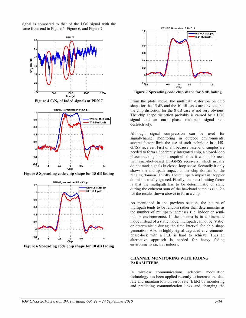
The C/N0 values of faded signals from a low elevation
satellite (PRN 07) are plotted in Figure 4. Three time
spans associated with 15 dB, 10 dB and 8 dB fading are
identified. The compressed chip shape for each case is
generated by coherently accumulating 2 s of baseband
samples after phase-lock. The chip shape of the faded
ION GNSS 2010, Session B4, Portland, OR, 21 – 24 September 2010 5/14
signal is compared to that of the LOS signal with the
same front-end in Figure 5, Figure 6, and Figure 7.
Figure 4 C/N0 of faded signals at PRN 7
Figure 5 Spreading code chip shape for 15 dB fading
Figure 6 Spreading code chip shape for 10 dB fading
Figure 7 Spreading code chip shape for 8 dB fading
From the plots above, the multipath distortion on chip
shape for the 15 dB and the 10 dB cases are obvious, but
the chip distortion for the 8 dB case is not very obvious.
The chip shape distortion probably is caused by a LOS
signal and an out-of-phase multipath signal sum
destructively.
Although signal compression can be used for
signal/channel monitoring in outdoor environments,
several factors limit the use of such technique in a HS-
GNSS receiver. First of all, because baseband samples are
needed to form a coherently integrated chip, a closed-loop
phase tracking loop is required; thus it cannot be used
with snapshot-based HS-GNSS receivers, which usually
do not track signals in closed-loop sense. Secondly it only
shows the multipath impact at the chip domain or the
ranging domain. Thirdly, the multipath impact in Doppler
domain is totally ignored. Finally, the most limiting factor
is that the multipath has to be deterministic or static
during the coherent sum of the baseband samples (i.e. 2 s
for the results shown above) to form a chip.
As mentioned in the previous section, the nature of
multipath tends to be random rather than deterministic as
the number of multipath increases (i.e. indoor or semi-
indoor environments). If the antenna is in a kinematic
mode instead of a static mode, multipath cannot be ‘static’
or deterministic during the time interval for chip shape
generation. Also in highly signal degraded environments,
phase-lock with a PLL is hard to achieve. Thus an
alternative approach is needed for heavy fading
environments such as indoors.
CHANNEL MONITORING WITH FADING
PARAMETERS
In wireless communications, adaptive modulation
technology has been applied recently to increase the data
rate and maintain low bit error rate (BER) by monitoring
and predicting communication links and changing the

ION GNSS 2010, Session B4, Portland, OR, 21 – 24 September 2010 6/14
modulation scheme adaptively. One of the key metrics
typically used in adaptive modulation technology for
evaluating communication links is the signal fading level,
which can be measured by the Ricean K-factor.
Ricean K-factor estimators generally can be categorized
into three groups: envelope-based estimators,
envelope/phase-based estimators, and phase-based
estimators. Six Ricean K-factor estimators and their
theoretical performance are briefly introduced in this
section.
Envelope-based Ricean K-factor Estimators
As shown by Tepedelenlioglu et al. (2003), at least two
different moments are required to estimate the Ricean K-
factor with envelope information only. The n th moment
can be estimated by averaging in a moving window
of N samples as:
1
0
1ˆ .
Nn
n i
i
rN
µ−
=
= ∑ (8)
Suppose n m≠ , the function ( ),n mf ⋅ and its inverse
function ( )1,n mf− ⋅ are defined as (Tepedelenlioglu et al.
2003):
( ), : .mn
n m nm
f Kµ
µ= (9)
1, ,
ˆˆ :
ˆ
mn
n m n m nm
K fµ
µ
−
=
(10)
The common choices for ( ),n m are ( )1, 2 and ( )2, 4 .
The corresponding ( ),n mf ⋅ functions are as follows
(Tepedelenlioglu et al. 2003):
( )( )
( )
( )
2
1, 2 0 1
2
14 1 2 2
1
Ke K Kf K K I KI
K
g K
K
π − = + +
+
= +
(11)
( )( )
22
2, 4 2
1
4 2
Kf K
K K
+ = + +
(12)
To estimate the Ricean K-factor, Equation (11) or (12)
need to be inverted. As shown by Azemi et al. (2003),
( )g K in Equation (18) can be approximated by a linear
or a quadratic polynomial with coefficients computed by
curve fitting:
( )1 1 0
1 01.000, and 0.7513
g K a K a
a a
= +
= = (13)
( ) 22 2 1 0
92 1 08.3285 10 , 1.000, and 0.7527
g K b K b K b
b b b−
= + +
= × = =
(14)
Therefore the Ricean K-factor can be estimated with 1st
and 2nd
moments based on a first order and a second order
approximation as follows (Azemi et al. 2003):
st
10
21, 2,1
11
2
ˆ
ˆˆ
ˆ
ˆ
a
K
a
µ
µ
µ
µ
−
=
−
(15)
nd
2
1 1 11 1 2 0
2 2 2
1, 2, 22
ˆ ˆ ˆ4
ˆ ˆ ˆˆ .
2
b b b b
Kb
µ µ µ
µ µ µ
− + − + −
=
(16)
Since 0K ≥ , from Equation (12), the Ricean K-factor
can be estimated with 2nd
and 4th
moments
(Tepedelenlioglu et al. 2003):
2 22 4 2 2 4
2, 4 22 4
ˆ ˆ ˆ ˆ ˆ2 2ˆ
ˆ ˆK
µ µ µ µ µ
µ µ
− + − −=
− (17)
Envelope/Phase-based Ricean K-factor Estimators
In some applications, coherent tracking is possible; thus
both phase and envelope information is available for
Ricean K-factor estimation. As shown by Chen &
Beaulieu (2005), the probability density function of the
fading envelope and fading phase is given by:
( )( )2 2
0, 2 2
2 cos, expr
r A rArp rθ
θ θθ
πσ σ
+ − − = −
(18)
where 0θ is the LOS phase (assuming to be constant
during averaging), r is the envelope of signals, θ is the
phase of signals, A is the LOS signal amplitude, and 2σ is the multipath power.

ION GNSS 2010, Session B4, Portland, OR, 21 – 24 September 2010 7/14
Assuming N independent and identically distributed
fading channel samples are available, the maximum
likelihood estimator (MLE) for Ricean K-factor can be
obtained by maximizing the log-likelihood function. Chen
& Beaulieu (2005) derived the MLE as follows:
{ }
{ }
1 11 10
1 1
sin
ˆ tan tan
cos
N N
k k k
k k
N N
k k k
i i
r P
r P
θ
θ
θ
− −= =
= =
ℑ
= =
ℜ
∑ ∑
∑ ∑ (19)
( ) { }0ˆ
0
1 1
1 1ˆ ˆcos
N Nj
k k k
k k
A r P eN N
θθ θ −
= =
= − = ℜ∑ ∑ (20)
2 2 2 2
1 1
1 1ˆ ˆˆN N
k k k
k k
r A P P AN N
σ ∗
= =
= − = −∑ ∑ (21)
2
2
ˆˆ
ˆMLE
AK
σ= (22)
where 0θ̂ is the estimated LOS phase (assuming to be
constant during averaging), kr is the envelope of signals,
kθ is the phase of signals, kP is the prompt correlation,
and N is the number of samples for averaging.
As shown by Baddour & Willink (2007), the MLE has a
bias of { } ( ) ( )ˆ 2 1 2MLE
K K K NΕ − = + − , but it
becomes asymptotically unbiased when a large number of
samples are used for averaging. Hence an unbiased
version of the MLE for finite samples:
( )1ˆ ˆ2 1MML MLK N KN = − −
(23)
where N is the number of samples for averaging.
Phase-based Ricean K-factor Estimators
By integrating the envelope argument, the probability
density function with only phase argument can be shown
as (Chen & Beaulieu 2005):
( )( ) ( )
( )( )
20sin0
0
cos
2 2
erfc cos
KKKe
p e
K
θ θθ
θ θθ
π π
θ θ
−− −−
= +
⋅ − −
(24)
where ( )erfc ⋅ is the complementary error function.
The approximate MLE which maximizes the log-
likelihood function for relatively large K is as follows
(Chen & Beaulieu 2005):
( )20
1
ˆ
ˆ2 sin
AML N
i
k
NK
θ θ=
=
−∑
(25)
where 0
1
1ˆN
k
kN
θ θ=
= ∑
Theoretical Performance of the Ricean K-factor
Estimators
To access the performance (the bias and the standard
deviation) of the estimators introduced above at different
C/N0 and K-factor values, a Monte-Carlo simulation was
done at the correlation level with a moving window of
100 samples (correlation values). In this simulation,
additive white Gaussian noise (AWGN) and Ricean
fading were added into the deterministic LOS signals. The
LOS signal phase was set to be a constant; the signal
Doppler and the spatial correlation between consecutive
samples were ignored.
From Figure 8 to Figure 11, the bias and the standard
deviation values for all estimators are plotted in solid
lines and dashed lines respectively with various C/N0
values, K-factor values and coherent integration times. A
negative bias appears for all estimators when the post-
correlation SNR is low due to low C/N0 and/or short
coherent integration, and the value of K-factor is
relatively large. Since the model used in the K-factor
estimation does not include the impact of AWGN, this
negative bias represents the impact of AWGN on the K-
factor estimation. If the post-correlation SNR is low while
the K value is relative large, meaning the level of AWGN
compared to Ricean fading is large; AWGN has
significant impact on the variation of the prompt
correlation’s envelope, which cannot be neglected.
Therefore the estimated K-factor is smaller compared to
the true value. It can be also observed that the standard
deviation increases as the K-factor increases. Similar to
the results from Chen & Beaulieu (2005) and Baddour &
Willink (2007), the MML and the MLE outperform
others. However, the difference is not large at all,
especially for GNSS signal/channel monitoring. One
point to bear in mind is that any phase-based K-factor
estimator assumes that the LOS signal phase is a constant
while the variation of the phase estimate is due to the
NLOS signals. Since the actual LOS phase of GNSS
signals is not a constant due to the motion and instability
of oscillators, phase tracking or highly precise frequency
tracking in a short duration is required to maintain a

ION GNSS 2010, Session B4, Portland, OR, 21 – 24 September 2010 8/14
‘stable’ phase. However the residual or the variation of
this ‘stable’ phase is not due to multipath only but the net-
effect of many other factors such as motion. Also a higher
post-correlation SNR is required for precise phase
estimation than for envelope estimation. Therefore
envelope based estimators are more robust and easier to
use than the others since they only require the envelope
information, which are available in any type of GNSS
receivers.
Figure 8 Performance of K-factor estimators with 100
ms coherent integration at 35 dB-Hz
Figure 9 Performance of K-factor estimators with
1000 ms coherent integration at 35 dB-Hz
Figure 10 Performance of K-factor estimators with
500 ms coherent integration at 45 dB-Hz
Figure 11 Performance of K-factor estimators with
500 ms coherent integration at 25 dB-Hz
SIGNAL MONITORING AND CHANNEL
CONTEXT DETECTION IN THE REAL WORLD
In the last two sections, signal compression and fading
parameters monitoring were introduced for signal/channel
monitoring. In this section, the results and analyses from
two experiments are presented. The first experiment was
conducted to assess the applicability and the consistency
of the Ricean K-factor estimation for GNSS signals. The
main purpose of the second experiment is to validate the
performance of the signal compression and fading
parameter estimation approaches for signal monitoring
and channel context detection in practice.
Experiment1: K-factor indoors and outdoors
To assess the performance of the K-factor estimators
indoor and outdoor with live GNSS signals (GPS L1 C/A
signals in this case), a static antenna was placed on the top
of a wooden house while another static antenna was in the
house. An NI front-end was used to collect data from both
channels at the same time. The software GNSS receiver

ION GNSS 2010, Session B4, Portland, OR, 21 – 24 September 2010 9/14
developed at the University of Calgary, GSNRxTM
(O’Driscoll et al. 2009), was used to process the data. In
both cases, phase-lock can be maintained.
The estimated C/N0 and K-factor outdoors and indoors are
shown from Figure 12 to Figure 15. As shown in these
plots, the K-factor can clearly reflect the signal strength
difference between indoor and outdoor. Although the
estimates from each group of estimators (i.e. envelope-
based) match well, a bias surprisingly exists between any
two groups of estimators. In other words, the fading
statistics from the envelope and the phase are not exactly
the same. As discussed in the previous section, the
residual phase, which is the tracking jitter of a PLL or the
accumulated tracking jitter of a FLL, is due to not only
multipath but also noise, signal dynamics, oscillator
instability, and tracking loop performance. In addition,
signal phase estimation is highly affected by noise.
Therefore an envelope-based K-factor estimator seems to
be a better choice for a GNSS receiver. In order to
understand this bias or validate the thought above, more
experiments and analyses are needed.
Figure 12 C/N0 from a static antenna outdoor
Figure 13 K-factor from a static antenna outdoor
Figure 14 C/N0 from a static antenna indoor
Figure 15 K-factor from a static antenna indoor
Experiment2: Channel Monitoring and Context Detection from Outdoor to Indoor
In order to validate the performance of signal
compression and fading parameter estimation approaches
for signal monitoring and channel context detection in
practice, the second experiment was conducted. In this
experiment, a static antenna named ‘reference’ was placed
on the top of a wooden house while another antenna
named ‘rover’ was held by a pedestrian outdoors. The
‘rover’ first remained stationary for about 60 seconds.
Then it was moved into the first floor of the house, down
to the basement, back outdoors for a while, and then
finally back to the first floor of the house. Both outdoor
and indoor signals were processed simultaneously by a
modified version of the GSNRxTM
software receiver
called GSNRx-rrTM
. The processing architecture of
GSNRx-rrTM
is shown below. Basically it processes
outdoor signals by a standard tracking loop to aid the
indoor channels via navigation data bits, carrier Doppler,
code phase, and carrier phase. Open-loop tracking is used
for indoor signal processing. In short, it is an AGPS type
of processing. For more details on this software, please
refer to Satyanarayana et al. (2010).

ION GNSS 2010, Session B4, Portland, OR, 21 – 24 September 2010 10/14
Figure 16 Processing architecture of GSNRx-rrTM
The data was processed with 100 ms, 500 ms, and 1 s of
coherent integration to investigate the impact of coherent
integration on signal parameter estimation and multipath
separation in frequency domain. The estimated rover
relative carrier Doppler and code phase with respect to the
reference estimates are plotted below. Clearly, the results
with 100 ms of coherent integration not only are noisy but
also fluctuate a lot in the local search domain compared to
the estimates from 500 ms and 1 s of coherent integration.
Figure 17 Rover relative carrier Doppler on PRN 22
Figure 18 Rover relative code phase on PRN 22
Figure 19 Rover relative carrier Doppler on PRN 11
Figure 20 Rover relative code phase on PRN 11
The estimated trajectories based on three different
coherent integrate times are show in Figure 21. A
standard Kalman filter was used in all three cases. The red
line, the green line, and the blue line represent the
estimated trajectory with coherent integration times 100
ms, 500 ms, and 1 s respectively. It can be observed that
some parts of the estimated trajectory (dots highline in
yellow) from 100 ms of coherent integration are totally
off from the building. Based on the time history, these
points should be within the area of the basement. After
examining the relative code phase and carrier Doppler
estimates associated with these points, it can be concluded
that the errors are due to the lack of sensitivity and
multipath errors. The estimated trajectories with 500 ms
and 1 s coherent integration times are reasonably
consistent. The epochs associated with the change of the
channel context (i.e. outdoor to indoor, indoor to outdoor)
were extracted from the trajectory with 1 s coherent
integration, since it should be the best one among all
three.

ION GNSS 2010, Session B4, Portland, OR, 21 – 24 September 2010 11/14
Figure 21 Estimated trajectories
As mentioned previously, the chip shape monitoring
approach may not be suitable in high signal degradation
environments. Chip shape was generated by 2 s of signal
compression based on standard closed-loop tracking. As
shown in Figure 22, the signal amplitude variation due to
the change of channel (i.e. outdoor to indoor) or loss of
lock of the close loop tracking can be easily observed,
however the chip shape distortion is hard to observe as
expected.
Figure 22 Chip shape from outdoor to indoor
The estimated C/N0 and K-factor values based on
envelope-based estimators with various coherent
integration times and moving window sizes are shown
below. Comparing the C/N0 and K-factor values on PRN
22, the mean value of C/N0 is approximately 40 dB-Hz
after the antenna moved indoors to the first floor, but the
C/N0 value varies from 53 dB-Hz to 28 dB-Hz in the case
of 100 ms coherent integration time. If the signal quality
or channel quality was indicated by the instantaneous
C/N0 value only, an optimistic decision might have been
made. In some literature, channel context such as indoor
or outdoor was detected or determined based on the
instantaneous C/N0 value only (Skournetou and Lohan
2007). Apparently this is too optimistic as shown in
Figure 23 and Figure 25. In order to monitor the
signal/channel and detect the channel context, the
indicator must be able to reflect the fading level over a
short duration of time. As shown in these figures, the K-
factor, which is a fading level indicator, performs very
well on signal/channel monitoring and detecting the
transition moving between outdoors and indoors.
Comparing the estimates from three envelope-based K-
factor estimators, the results from the two with 1st and 2
nd
moments are almost identical while the estimates from the
one with 2nd
and 4th
moments are much noisier and more
‘faded’ especially in the low C/N0 range. This is because
the noise is amplified more significantly in the 4th
moment estimation compared to the 1st moment
estimation. The performance difference between these
estimators can be reduced by utilizing a longer coherent
integration as shown in Figure 26.
Figure 23 C/N0 on PRN 22 with coherent integration
time 100 ms
Figure 24 K-factor on PRN 22 with coherent
integration time 100 ms

ION GNSS 2010, Session B4, Portland, OR, 21 – 24 September 2010 12/14
Figure 25 C/N0 on PRN 22 with coherent integration
time 1 s
Figure 26 K-factor on PRN 22 with coherent
integration 1 s
Figure 27 C/N0 on PRN 9 with coherent integration
time 500 ms
Figure 28 K-factor on PRN 9 with coherent
integration time 500 ms
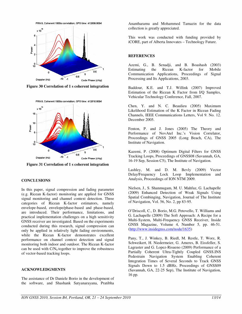
In this experiment, one interesting observation was the
multipath signal separation in frequency domain. After a
long coherent integration, the frequency resolution is very
high; therefore, the direct signal and specular multipath
components can be separated. This phenomenon is
illustrated from Figure 29 to Figure 31. Therefore, in a
vector-based tracking loop operating in a kinematic mode,
the LOS signals can be separated from NLOS signals by
comparing the Doppler values of all peaks with the
estimated Doppler value predicted from the navigation
solution after a long enough coherent integration.
Figure 29 Correlation of 1 s coherent integration
ION GNSS 2010, Session B4, Portland, OR, 21 – 24 September 2010 13/14
Figure 30 Correlation of 1 s coherent integration
Figure 31 Correlation of 1 s coherent integration
CONCLUSIONS
In this paper, signal compression and fading parameter
(e.g. Ricean K-factor) monitoring are applied for GNSS
signal monitoring and channel context detection. Three
categories of Ricean K-factor estimators, namely
envelope-based, envelope/phase-based and phase-based,
are introduced. Their performance, limitations, and
practical implementation challenges on a high sensitivity
GNSS receiver are investigated. Based on the experiments
conducted during this research, signal compression can
only be applied in relatively light fading environments,
while the Ricean K-factor demonstrates excellent
performance on channel context detection and signal
monitoring both indoor and outdoor. The Ricean K-factor
can be used with C/N0 together to improve the robustness
of vector-based tracking loops.
ACKNOWLEDGMENTS
The assistance of Dr Daniele Borio in the development of
the software, and Shashank Satyanarayana, Pratibha
Anantharamu and Mohammed Tamazin for the data
collection is greatly appreciated.
This work was conducted with funding provided by
iCORE, part of Alberta Innovates – Technology Future.
REFERENCES
Azemi, G., B. Senadji, and B. Boashash (2003)
Estimating the Ricean K-factor for Mobile
Communication Applications, Proceedings of Signal
Processing and Its Applications, 2003.
Baddour, K.E. and T.J. Willink (2007) Improved
Estimation of the Ricean K Factor from I/Q Samples,
Vehicular Technology Conference, Fall, 2007.
Chen, Y. and N. C. Beaulieu (2005) Maximum
Likelihood Estimation of the K Factor in Ricean Fading
Channels, IEEE Communications Letters, Vol 9. No. 12.
December 2005.
Fenton, P. and J. Jones (2005) The Theory and
Performance of NovAtel Inc.’s Vision Correlator,
Proceedings of GNSS 2005 (Long Beach, CA), The
Institute of Navigation.
Kazemi, P. (2008) Optimum Digital Filters for GNSS
Tracking Loops, Proceedings of GNSS08 (Savannah, GA,
16-19 Sep, Session C5), The Institute of Navigation.
Lashley, M. and D. M. Bevly (2009) Vector
Delay/Frequency Lock Loop Implementation and
Analysis, Proceedings of ION NTM 2009.
Nielsen, J., S. Shanmugam, M. U. Mahfuz, G. Lachapelle
(2009) Enhanced Detection of Weak Signals Using
Spatial Combinging, Navigation, Journal of The Institute
of Navigation, Vol. 56, No. 2, pp 83-95.
O’Driscoll, C., D. Borio, M.G. Petovello, T. Williams and
G. Lachapelle (2009) The Soft Approach: A Recipe for a
Multi-System, Multi-Frequency GNSS Receiver, Inside
GNSS Magazine, Volume 4, Number 5, pp. 46-51.
(http://www.insidegnss.com/node/1635)
Pany, T., J. Winkey, B. Riedl, M. Restle, T. Worz, R.
Schweikert, H. Niedermeier, G. Ameres, B. Eissfeller, S.
Lagraster and G. Lopez-Risueno (2009) Performance of a
Partially Coherent Ultra-Tightly Coupled GNSS.INS
Pedestrain Navigation System Enabling Coherent
Integration Times of Several Seconds to Track GNSS
Signals Down to 1.5 dBHz, Proceedings of GNSS09
(Savannah, GA, 22-25 Sep), The Institute of Navigation,
16 pp.

ION GNSS 2010, Session B4, Portland, OR, 21 – 24 September 2010 14/14
Pany, T. and B. Eissfeller (2006) Use of a Vector Delay
Lock Loop Receiver for GNSS Signal Power Analysis in
Bad Signal Conditions, in ION Annual Meeting/IEEE
PLANS, San Diego, CA.
Petovello, M.G., C. O'Driscoll and G. Lachapelle (2008)
Weak Signal Carrier Tracking Using Extended Coherent
Integration with an Ultra-Tight GNSS/IMU Receiver,
Proceedings of European Navigation Conference
(Toulouse, 23-25 April), 11 pages.
Petovello, M.G. and G. Lachapelle (2006) Comparison of
Vector-Based Software Receiver Implementations With
Application to Ultra-Tight GPS/INS Integration.
Proceedings of GNSS06 (Forth Worth, 26-29 Sep,
Session C4), The Institute of Navigation, 10 pages.
Satyanarayana, S., D. Borio and G. Lachapelle (2010)
Power Levels and Second Order Statistics for Indoor
Fading Using a Calibrated A-GPS Software Receiver.
Proceedings of GNSS10 (Portland, OR, 21-24 Sep,
Session E1), The Institute of Navigation.
Schmid, A., C. Gunther, and A. Neubauer (2005) Rice
Factor Estimation for GNSS Reception Sensitivity
Improvement in Multipath Fading Enviroments,
Proceedings of the 2nd
Workship on Positioning,
Navigation and Communication, 2005.
Skournetou, D., and E. S. Lohan, Indoor location
awareness based on the non-coherent correlation function
for GNSS signals, In Proc. Of Finnish Signal Processing
Symposium (FINSIG 07), Oulu, Finland, August 2007
Tepedelenlioglu, C., A. Abdi, and G. B. Giannkis (2003)
The Ricean K Factor: Estimation and Performance
Analysis, IEEE Transactions on Wireless
Communications, Vol. 2, No. 4, July 2003.
Weil, L. (2007) Theory and Applications of Signal
Compression in GNSS Receivers, in Proceedings of ION
GNSS ITM07.