Changing Patterns in Household Ownership of Municipal Debt: Evidence from the 1989-2013 Surveys of Consumer Finances

Daniel Bergstresser* Randolph Cohen**

(First draft May, 2015. Current draft June, 2015. Comments welcome)

Abstract

The period since 1989 has seen significant changes in the structure of household ownership of municipal debt, with ownership becoming concentrated in a smaller number of households over time. The share of households holding any municipal debt fell from 4.6 percent to 2.4 percent between 1989 and 2013. The share of total debt that is held by the wealthiest 0.5 percent of households rose from 24 percent to 42 percent over the same period. These changes have coincided with the growth of tax-deferred retirement investment accounts such as 401(k) plans as a primary location of household investing. Municipal bonds, which pay tax-exempt interest, are almost never held inside of these tax-deferred accounts. These changing patterns of ownership have implications for the political economy of the municipal bond market.

Keywords: Municipal bonds.

We are grateful for support from the Brandeis International Business School. * Corresponding author. Brandeis International Business School. dberg@brandeis.edu. ** MIT.

1

 

Municipal bonds have historically been an extremely safe investment, with defaults for

rated municipal issuers averaging 0.01 percent per year during 1970-2007 and still only 0.03

percent per year over the more turbulent 2008-2013 period (Moody’s, 2014).1 This safety has

made the debt attractive as an investment for many households, and direct investment by

households has been an important part of the ownership structure of municipal debt. Municipal

debt markets also often have a local flavor, with households disproportionately investing in debt

from issuers in their own states (Kidwell et al, 1984). There is an interplay between safety and

breadth of direct holding – repayment of municipal debt is based in part on the political will of

the issuer to repay, and a broad base of holders who are directly exposed to an issuer’s municipal

debt creates a significant constituency that can be counted upon to support repayment.2

But the structure of household ownership of municipal debt appears to be changing over

time, and in ways that are not visible in aggregate statistics. In this paper we use household data

from the 1989 through 2013 Surveys of Consumer Finances to look at disaggregated data on

municipal debt ownership. A clear picture emerges: the share of households holding municipal

bonds appears to be shrinking significantly over time. Household ownership rates have fallen

from 4.6 percent to 2.4 percent. This drop in ownership rates has occurred even though

aggregate household holdings of municipal debt have increased over time. Municipal bond

ownership is becoming concentrated in a smaller and smaller number of hands.

When we look at changing patterns of ownership of other assets, for example shares of

stock and holdings of other bonds, we find that municipals are unusual in their falling household

                                                            1 A recent study by the Federal Reserve Bank of New York (Appleson et al, 2012) found (not surprisingly) much higher default rates among the set of bonds that do not carry ratings. 2 In the end, households own all of the assets in the economy. Corporate bonds are often owned by insurance companies, which are in turn often owned in part by mutual funds, and those funds are owned by households. But the link from the issuer to the household is particularly direct in the municipal bond market.

2

 

ownership rates. The share of households owning any stock has risen from 27.3 percent to 42.7

percent since 1989, and the share of households owning any non-municipal bonds has risen from

45.3 percent to 46.8 percent. But the location of household investing has shifted since 1989

toward tax-deferred accounts such as 401(k)s, 403(b)s, and IRAs. Municipal bonds’ tax-

exemption reduces their pre-tax yields and makes them a very unusual (and even inappropriate)

asset for tax-deferred accounts. So the declining ownership rates for municipal bonds have

coincided with a shift in household portfolios towards accounts where municipals are a tax-

disadvantaged investment.

When we fit empirical models explaining the determinants of the household decision to

hold bonds, more interesting patterns emerge. In particular, the drivers of household municipal

bond holdings have changed over time. In 1989, family income was a very strong predictor of

ownership of municipal bonds, as was a household’s estimated marginal tax rate. The relative

predictive power of net worth and income has changed over time: by 2013 net worth was a much

stronger predictor of owning municipal bonds. Conditional on net worth, higher-income

households are no longer more likely than lower-income households to own municipal bonds. In

addition, the share of household financial assets held through tax-deferred accounts is a strong

predictor in each survey of whether or not a household holds municipal bonds.

A number of market commentators have made extreme predictions about the prospects of

future municipal defaults. Meredith Whitney, for example, forecasted in 2010 that there would

be ‘hundreds of billions of dollars worth of defaults.’3 As we pointed out in earlier work

(Bergstresser and Cohen, 2011), our view is that Whitney’s and other similar predictions were

                                                            3 Meredith Whitney, interviewed on CBS’ 60 Minutes in December 2010: ‘There’s not a doubt in my mind that you will see a spate of municipal bond defaults…You could see 50 sizeable defaults. 50 to 100 sizeable defaults. More. This will amount to hundreds of billions of dollars worth of defaults.

3

 

extreme and reflected a poor understanding of the municipal market. Nonetheless, the security

of municipal bonds in the end rests on the political will of issuers to make hard choices and repay

their debt. Part of the reason why issuers have repaid their debt has been the political

constituency of municipal bond owners, who form a reliable voice in favor of repaying debt. We

thus view the declining ownership of municipal debt as cause for concern from a political

economy perspective.

Given the declining share of households who own municipal debt, another area of

potential concern is the municipal tax exemption. Tracing the economic effect of the tax

exemption through the economy is a complex exercise, and economic theory shows that the net

cost of a tax (or benefit of a subsidy) is not necessarily borne by the household directly paying

the tax. Recent work (Galper et al, 2014) suggests that some households who don’t own

municipal bonds benefit from the tax exemption through the exemption’s effect of subsidizing

the provision of public sector goods and services. Even so, a declining share of households who

hold municipal bonds and perceive themselves as benefiting from the tax exemption may place

this exemption on a shakier political foundation.

This paper proceeds in eight sections. The first section describes the Surveys of

Consumer Finances. The second section describes patterns of municipal debt ownership; a third

section breaks out debt held directly versus debt held through mutual funds. A fourth section

describes the concentration of municipal bond portfolios into a small number of households. A

fifth section describes the characteristics of municipal debt owners in the different waves of the

survey. A sixth section describes our approach to calculating statistical confidence measures for

our estimates, a seventh section fits probit models predicting household municipal ownership,

and a final section concludes.

4

 

1. The Surveys of Consumer Finances

The Survey of Consumer Finances (SCF) is a survey of US households, conducted every

three years by the Federal Reserve Board, in cooperation with the Internal Revenue Service. The

modern incarnation of the survey began in 1983, and the questionnaire and sample design have

been relatively stable since 1989, allowing comparison across surveys in different years. Since

that time the survey has been constructed as a repeated cross-section rather than as a panel study

following the same household across different surveys.4 The SCF is widely used by academic

and government researchers studying household portfolio choice and related decisions. SCF data

are regarded as the most reliable and extensive data on household wealth available for the United

States (Dettling and Hsu, 2014).

A key feature of the SCF is the dual-frame sampling design (Kennickell, 2005). The

dual-frame design means that part of the sample comes from an area-probability sample and a

second part comes from what is called the ‘list sample.’ The area-probability sample represents

about 2/3 of the total sample, and is constructed through geographically stratified sampling of a

national sampling frame developed by the National Opinion Research Center (NORC) at the

University of Chicago. The list sample is used to over-sample households likely to be wealthy,

and is based on a sample of individual tax returns developed by the IRS’ Statistics of Income

(SOI) Division.

Over-sampling wealthy households is particularly important given that wealth is

concentrated in a relatively small number of households. The combination of an area-probability

sample with a list-sample which over-samples the wealthy means that the SCF can be used to

                                                            4 An exception to this was a 2009 re-survey of 2007 survey households. This re-survey was designed to assess household assets and income across the financial crisis.

5

 

investigate both behaviors that are widely distributed in the population (for example use of credit

cards) and behavior that is more concentrated in the very wealthy (for example ownership of

stock or mutual funds.) In our context, the sample design means that the same survey is useful

both for investigating the share of households that have municipal debt and also the structure of

municipal debt ownership among the relatively small number of households that own municipal

bonds.

The SCF is distinguished by its high level of detail on the disaggregated components of

wealth. This disaggregation means that the survey is particularly useful for investigating

questions around household portfolio shares in different assets (Poterba and Samwick, 2003),

and can be used as well to investigate household assets held both inside and outside of tax-

deferred accounts such as defined contribution pension plans (Bergstresser and Poterba, 2004).

For example, the SCF asks questions both about municipal bonds held directly and also about

tax-exempt municipal bond mutual funds, a feature that we exploit in this work. The SCF also

asks demographic questions, for example household composition, ages, educational status, and

occupational and employment status.

SCF observations come with analysis weights that are intended to specify the number of

households in the larger population that are similar to the survey household (see Kennickell and

Woodburn, 1999). These analysis weights can be thought of as representing the inverse of the

probability of selection of a household into the sample. The weights allow researchers using the

survey to address questions such as the distribution of wealth ownership in the population from

which the survey is drawn, which is the population of US households.

6

 

A key feature of the SCF is the use of multiple imputation for handling nonresponse in

the survey. Rubin (1987) gives details on multiple imputation in surveys, and Kennickell (1999)

describes the use of multiple imputation in the SCF. As with any survey, some households in the

SCF decline to answer certain questions about aspects of wealth or income, or are only willing to

give answers indicating a range for a given variable rather than a dollar amount. Table 1 (based

very closely on Kennickell, 1999) shows data on nonresponse and range response from the 1995

SCF. Some items have very high response rates, for example the variable capturing household

payment of rent. On an unweighted basis, 23.8 percent of households reported paying rent, and

no households reported being unsure whether or not they paid rent. Of the households that report

paying rent, 95.1 percent gave a number for the dollar amount of rent that they paid, and 4.3

percent gave a range. No households reported paying rent and not knowing how much they paid,

and 1.5 percent of the observations were coded as ‘missing.’ For many variables, the bulk of the

missing reflects refusals by the household to give a dollar figure, but in some cases it reflects an

editing decision on the part of the Federal Reserve staff (hence delivering four categories that

some to more than 100 percent.)

For municipal bonds rates of refusal by survey respondents were higher. On an

unweighted basis, 8.1 percent of households reported having municipal bonds. Because the

survey oversamples wealthy households, this share with municipal bonds in the raw sample is

higher than the rate implied for the population from which the sample was drawn. 1.2 percent of

households report not knowing whether they owned municipal bonds or not, or were otherwise

unable or unwilling to answer the question.5 Of the households that were willing and able to

reveal that they owned municipal bonds, almost eighty percent were able and willing to give at

                                                            5 For example, one household (out of 4299) had broken off the survey by that point, but had provided enough information before breaking the survey off to be included as a participant in the survey.

7

 

least a range for the value of their holdings. 1.2 percent reported not knowing the value of their

holdings, and 20.1 percent were unwilling or otherwise unable to provide a value.

The SCF handles these missing observations using an imputation approach, meaning

that missing observations are re-coded with values based on the sampling distribution of the

variable and the characteristics of the household for which the data are missing. This approach is

standard practice in use of household survey data and minimizes bias and statistical inefficiency

due to survey nonresponse. It has been recognized (see Rubin (1987) and Montalto and Sung

(1996)) that although single imputation, where missing observations are replaced in the dataset

based on household characteristics, minimizes bias, single imputation leads to systematic

underestimates of the variability in the data because the imputed values for the missing

observations are treated as if they were known with certainty. For this reason, the SCF uses a

multiple imputation approach. From each underlying household observation the survey creates

five ‘implicates,’ each based on that household. The imputed variables in the five implicate

datasets can be given both the appropriate mean and also a variance that corrects for the

uncertainty given the missing values.

This multiple imputation approach means that some care must be taken in assessing the

statistical significance of econometric results when using SCF data. For example, in the 1995

survey, the 21,495 implicate observation in the dataset are based on 4,299 underlying

households. This means that the statistical confidence of regressions (for example our probit

regressions in this paper) is lower than naïve analysis based on the 21,495 observations would

imply. We therefore follow the practice recommended by the SCF staff, based on Rubin (1987),

8

 

for calculating confidence intervals for our estimates presented in this paper.6 This approach is

described in more detail in the sections that follow.

Beyond non-response to individual questions, there is an issue in the SCF (and in any

survey) with non-response to the entire survey. According to Kennickell (1999), in 1995, 66

percent of the eligible area-probability sample participated in the survey, which is an astounding

level of participation given the high level of detail collected by the survey. One explanation for

the high participation rates is that potential participants receive a letter from the Chairman of the

Federal Reserve Board describing the importance of the survey and assuring potential

participants of the confidentiality of their responses.7 Participation rates for the wealthier list

sample are lower, with rates that varied from 44 percent in the lowest wealth stratum to 13

percent in the highest. Adjusting for non-participation involves adjustment of sampling weights,

a process that is made easier in the case of the list sample by the fact that at least some

information about nonparticipating households in the list sample is available from the Internal

Revenue Service.8

Table 2 describes the observations in the 1989-2013 surveys, cutting the data by the level

of financial assets.9 The 2013 survey data include 30,075 implicate observations; these

observations are based on 6,015 underlying households surveyed. Average financial assets in

                                                            6 See discussion of sampling error in the SCF codebook at http://www.federalreserve.gov/econresdata/scf/files/codebk2013.txt. That section of the codebook has code in the SAS programming language for calculating standard errors of estimates. Our analysis was performed using the Stata programming language, and we are grateful to Kevin Moore from the Federal Reserve Board staff for providing the Stata .ado-file used to calculate confidence intervals for the analysis in this paper. 7 The Chairman’s letter for the 2013 survey is available at http://www.federalreserve.gov/scf/bernankeletter2013.htm. 8 See Kennickell (1997) for more detail on unit nonresponse in the SCF. 9 Our measure of financial assets includes checking accounts, IRA accounts, CDs, savings accounts, money market accounts, savings bonds, publicly-traded stock, bonds, mutual funds, the cash value of whole life insurance, trusts, defined contribution pension plans, and a measure of ‘other funds,’ which according to SCF staff is mostly hedge funds. Assets excluded from our measure of financial assets include privately-held businesses, homes, and other real estate.

9

 

the entire population came to $225,136. Data in the table (as elsewhere in the paper) are

reported in 2013-equivalent dollars; data from 1989, for example, are inflated to a 2013-dollar

equivalent using the CPI-U levels in 1989 and 2013.10 Average inflation-adjusted financial

assets peaked in 2001, reflecting the peak of the internet bubble, at a level of $239,520 per

household. Financial assets grew rapidly between 1995 and 2001, but have fluctuated between

$211,000 and $226,000 between 2004 and 2013.

The total number of households in the population implied by the survey weights has

grown from 93,020,000 in 1989 to 122,530,000 in 2013. The vast majority of these households

have minimal financial assets. In 2013, 91 million households (74.3 percent of the total) had less

than $100,000 in financial assets, and the average level of financial assets among these

households was $16,128. At the same time, there has been rapid growth in the number of very

wealthy households. In 2013, survey data imply that 806,000 households had more than $5

million in financial assets, or 0.66 percent of all households, versus 0.18 percent of households

that were above this threshold in 1989. 4.2 percent of households in 2013 had financial assets

totaling to over a million dollars, up from 2.0 percent in 1989.

Table 3 presents the same data but with a different way of breaking apart observations,

cutting by the percentile of financial assets rather than by their absolute level. In this way the

share of households in each group remains constant across the survey years. This approach

demonstrates more starkly the stagnation in wealth in the bottom part of the distribution and the

growth in wealth at the top. Average financial assets in the bottom 50 percent of households was

$2,754 in 2013, down from $2,959 in 1989 (and $5,714 in 2001). The average among of

                                                            10 The CPI-U in 2013 was 233.0, and the CPI-U in 1989 was 124.0. By this measure, prices have grown by 88 percent over the 24 years between 1989 and 2013, or an average compounded growth rate of 2.6 percent.

10

 

financial assets in the top 0.5 percent of the population rose from $5.9 million in 1989 to $12.9

million in 2013. The finding that wealth has been stagnating at the bottom and rising at the top is

not new, and has been documented by other researchers, including researchers using SCF data

(Bricker et al, 2014).

2. Patterns of ownership of municipal debt, 1989-2013

An important feature of the municipal debt market is that political will plays an important

role in assuring that debt will be repaid. In a democracy, breadth of ownership of municipal debt

creates an important constituency that can be counted upon to advocate for debt repayment. In

this section we investigate the patterns of ownership of municipal debt using the 1989 through

2013 Surveys of Consumer Finances and find that ownership is becoming more concentrated,

with a small number of households holding a larger and larger share of the debt.

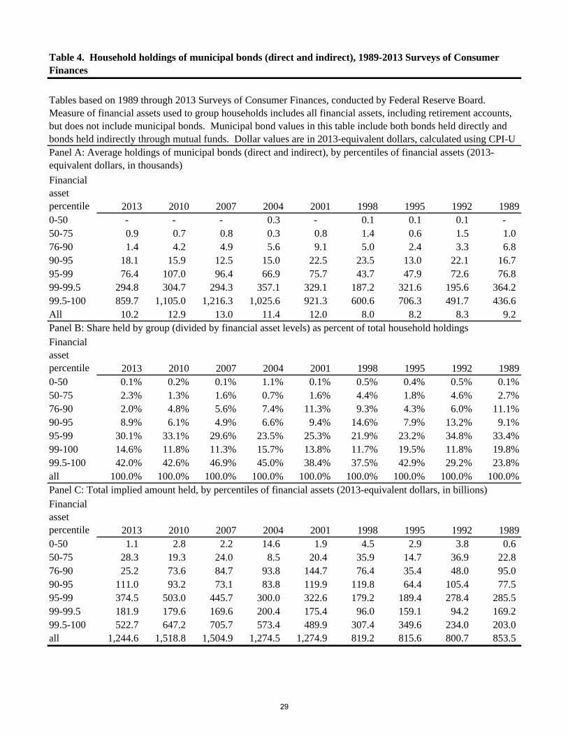
Table 4 shows patterns in household ownership of municipal debt, broken out by

percentiles of total financial assets, between 1989 and 2013.11 Panel A of the table shows the

average amount of municipal debt held, by group and by year. The measure of municipal debt

used in this table aggregates bonds held directly and bonds held indirectly, through tax-exempt

mutual funds. The average household held $10,200 in directly-held and indirectly-held

municipal bonds in 2013. Holdings per household in the survey peaked at $13,000 in 2007, and

reached a low point of $8,000 in 1998. Survey responses suggest that the average household in

the top 0.5 percent of the asset distribution held $859,700 worth of municipal debt in 2013, a

figure that was down somewhat from a peak of $1,216,300 in 2007 but up from $436,600 in

1989.

                                                            11 The measure of financial assets used to cut the sample into groups excludes municipal bonds and tax-exempt bond funds.

11

 

Panel B shows the share of municipal debt that is held by groups in different levels of

wealth between 1989 and 2013. The overall picture that emerges is that holdings of bonds have

become increasingly concentrated at the top of the distribution: the share held by the top 0.5

percent has risen from 23.8 percent in 1989 to 42.0 percent in 2013. Closer analysis of the data

shows that the change in the distribution has come in two phases. The top 0.5 percent gained

share between 1989 and 1995, but took that share in part from the households between the 95th

and 99th percentile of financial assets, as well as from households between the 75th and 90th

percentiles. In the second part of the sample, from 1995 and 2013, the share held between the

75th and 90th percentiles continued to fall. In 1989, 11.1 percent of municipal debt was held by

households between the 75th and 90th percentiles of financial assets; by 2013 that figure had

fallen to 2.0 percent.

Panel C of Table 4 shows the survey-implied total amounts of municipal bonds held in

different parts of the wealth distribution. Total holdings implied by the survey peak at $1,505

billion in 2007, and stood at $1,245 billion in 2013. These figures are somewhat lower than

figures implied by the Federal Reserve’s Flow of Funds statistics. According to the Flow of

Funds data, the household sector directly held $1,618.4 billion in municipal bonds in 2013. This

discrepancy could have a number of sources. For one thing, the ‘household sector’ in the Flow

of Funds data does not perfectly overlap with the sample frame of the Fed’s SCF. Another

consideration is that the data for the household sector in the flow of funds are calculated as a

residual, based on the total known stock of municipal bonds and the amounts known to be held

within other sectors that that the Flow of Funds data break out. The discrepancy could also

speak to some systematic underreporting of the level of municipal bond holdings by SCF survey

12

 

respondents. Antoniewicz (2000) and Henriques and Hsau (2013) describes known differences

between SCF data and Flow of Funds data.

Table 5 shows two different perspectives on the importance of municipal debt for

household portfolios. Panel A shows the share of households that report having any municipal

bonds (either held directly or held through mutual funds) in their portfolios. The share of

households reporting that they hold municipal bonds rose from 4.6 percent in 1989 to 4.8 percent

in 1998, but it has since fallen sharply and as of 2013 stands at 2.4 percent. Declines have

occurred at all levels of wealth, but the drops in the upper middle class are particularly large.

The share of households between the 75th and 90th percentiles of financial assets who report

holding municipal bonds fell has fallen from 9.6 percent in 1998 to 2.6 percent in 2013.

Between the 50th and 75th percentiles of financial assets, the share has fallen from 3.8 percent to

0.9 percent over the same time.

Panel B shows municipal debt as a share of household total financial portfolios at

different levels of financial assets. As a share of the total asset portfolio, municipal bonds have

fallen over time from 7.9 percent to 4.5 percent, although their share rose during periods of the

2000s, largely due to fluctuation in the value of household holdings of equities. Although there

is significant variation across different years of the survey, the decline in municipal bonds as a

share of financial assets in the 75th to 90th percentiles is stark: it has dropped from 5.2 percent to

0.6 percent. Speaking more generally, households between the 50th and 90th percentiles of assets

hold much less municipal debt (as a share of their assets) than they did in the past.

Table 6 compares the changing ownership rates of municipal debt to changing ownership

rates of a variety of other assets. For stock and non-municipal bonds, the table breaks out

13

 

ownership by the location of the assets – inside versus outside of tax-deferred accounts. A large

literature (including Bergstresser and Poterba, 2004) investigates household asset location

choices. A key result from this literature is that optimal asset location involves preferentially

holding highly-taxed assets inside of tax-deferred accounts. This asset location strategy

maximizes the implicit subsidy to the investor coming from the tax advantage of the tax-deferred

account. For a household to hold tax-exempt municipal bonds inside of a tax-deferred account

would contradict the most basic advice of the asset location literature, and such portfolio choices

are unlikely to be very common.12

The share of households owning any stock (either inside or outside of a tax-deferred

account) rose from 27.3 percent to 42.7 percent over the period since 1989. But the share of

households directly (as opposed to through a mutual fund) owning shares outside of a tax-

deferred account fell over the same period from 16.9 percent to 13.8 percent. The growth in

equity participation is entirely a consequence of growing equity participation inside of tax-

deferred accounts.

Ownership of non-municipal bonds (including savings bonds) has been more static, with

rates rising from 45.3 percent to 46.8 percent over the same period. A similar pattern emerges

with respect to asset location, with the share of households holding fixed income assets inside of

a tax-deferred account rising from 30.7 percent to 43.6 percent over the period, and the share of

households holding fixed income assets outside of a tax-deferred account falling from 28.3

percent to 12.5 percent over the same period. Over time, there appears to have been a shift in the

locus of household investing activity from outside to inside of tax-deferred retirement accounts, a

change that has coincided with a decline in the share of households holding municipal bonds.

                                                            12 The SCF only asks about holdings of municipal debt outside of tax-deferred accounts.

14

 

3. Municipal debt held directly and held through mutual funds

Our analysis so far has aggregated bonds held directly and bonds held through tax-

exempt mutual funds. In this section we break these components apart, and some interesting

patterns emerge. The main theme is that the decline in the share of households owning any

municipal debt is particularly pronounced when we focus on the households who hold that debt

directly, as opposed to holding in indirectly through tax-exempt bond funds.

Panel A of Table 7 shows the share of households in the various waves of the Survey of

Consumer Finances that report holding municipal bonds directly. The 1989 survey data suggest

that 3.5 percent of households directly held bonds, a share that appears to have fallen below 1

percent as of the 2013 survey. Direct ownership of municipal bonds has been falling across the

distribution of financial assets. At the top, ownership rates are large but falling: the share of

households in the top 0.5 percent holding bonds directly fell from 42.6 percent to 29.4 percent.

Ownership rates in the next 0.5 percent – households whose financial asset holdings place them

in the 99th to the 99.5th percentiles – fell from 58 percent in the 1989 survey to 16.2 percent in

2013. Rates of ownership in the upper middle class have fallen as well, and have fallen from

lower initial levels. The rate of ownership by households in the 90th to 95th percentiles has fallen

from 13.0 percent to 2.3 percent over the same period. Direct ownership of municipal bonds

used to penetrate well into the middle class: in 1989 the rate of ownership by the 50th-75th

percentile households was 1.9 percent. The same figure that was only 0.3 percent as of 2013.

Panel B of Table 7 shows direct holdings of municipal debt as a share of total financial

assets, again partitioned by household levels of financial assets. Note again that the measure of

financial assets used to partition households excludes municipal debt. Direct ownership of

15

 

municipal debt as a share of financial assets was 9.5 percent in the 99th-99.5th percentile

households in 1989, and had fallen to 3 percent by 2013. For the sample as a whole, direct

holdings of municipal debt fell from 5.8 percent to 2.7 percent across the nine waves of the

survey that we use in this paper.

Table 8 shows ownership rates and levels for tax-exempt bond mutual funds, and a

somewhat different picture emerges. Ownership rates of municipal bond funds rose between

1989 and 1998 from 1.5 percent of households to 3.5 percent of households. This expansion of

ownership reflected the larger move towards mutual funds as a focus of household investing.

But fund ownership rates have fallen since 1998, and now stand at 1.6 percent of all households.

This pattern repeats across each of the asset level categories. For example, among the

households at the 90th-95th percentiles of financial assets, ownership rates rose from 5 percent to

12.2 percent before falling back down to 5.2 percent by 2013. Municipal bond funds as a share

of total financial assets (Panel B of Table 7) have been relatively stable, ranging from 1.6 percent

to 2.5 percent of total financial assets. The overall picture that emerges from this disaggregated

analysis is that the decline in direct ownership of municipal debt has been much more rapid than

the decline of intermediated household ownership.

4. The concentration of municipal debt ownership

In this section we investigate further the degree to which municipal bond holdings are

concentrated in a very small number of households, and the extent to which that concentration

has changed over time. Table 9 returns to focusing on measures of municipal debt ownership

that aggregate direct and indirect holdings. The top row of the table, repeating information

described earlier, shows the share of all households in the sample that report owning any

16

 

municipal debt. That share has fallen to 2.4 percent as of 2013. Panel A of the table focuses just

on the households owning municipal debt and shows the distribution of ownership levels within

these households. Among households owning municipal debt, the median ownership level in

2013 was $70,000. The distribution is highly and increasingly skewed. The mean ownership

level among households owning municipal bonds was $432,000 in 2013, up from $200,000 in

1989. As figure B shows, the vast majority of the bonds are held by the small number of

households who hold municipal bonds in large amounts. The share of debt held by the top 50

percent of debt holders (among those who hold municipal bonds) rose from 95.1 percent in 1989

to 97.4 percent in 2013. Combining these numbers with the declining overall ownership rates

means that in 1989 the top 2.3 percent of all households (ranking by municipal ownership) held

95.1 percent of the debt, while in 2013 the top 1.2 percent of households held more than 97

percent of the debt. Almost 90 percent of the debt was held by the top 25 percent of municipal

owners. With the declining ownership rates of municipal debt, these top 25 percent of owners

now represent only 0.6 percent of households in the population. Ownership of municipal debt in

large quantities is becoming more and more concentrated in a very small number of households.

5. Evidence on the characteristics of municipal bond owners

In this section we present evidence on the characteristics of the municipal bond owning

community. We start by focusing on their age. One hypothesis, given our earlier results on the

declining share of households that own municipal bonds, would be that the set of municipal bond

owners is shrinking because it is aging and not being replenished with new bond owners over

time. But Table 10 suggests that other factors are at work. Between 1989 and 2013 the age

profile of municipal debt owners have been remarkably stable, with median and mean ages

around 60 years. This stability contrasts with an aging overall population: the average age of the

17

 

households that do not own municipal bonds has risen from 47 to 51 years over the same period,

and the median age has risen from 44 years to 50 years.

Municipal debt is a particularly attractive asset for households that face high marginal tax

rates on their income; this relative tax advantage to tax-exempt income is greater at higher tax

rates. Table 11 shows the distribution of marginal tax rates for households, partitioned by

municipal bond ownership status. Our marginal tax rate estimate comes from linking the SCF

data with the NBER’s TAXSIM tax simulator (Feenberg and Coutts, 1993). This calculator,

when given household characteristics and income levels, will return federal marginal tax rates.

We are unable to calculate marginal state tax rates because the public-use SCF files do not have

information on the geographical location of the households in the survey.13 Effective tax rates

can be negative in certain regions of the income distribution due to the phase-in of the Earned

Income Tax Credit (EITC), which provides a subsidy for work which is based on income.

Effective marginal tax rates become extremely high in regions of income where the EITC

benefits are being phased out.

Not surprisingly, the SCF data suggest that the community of municipal bond owners is

characterized by higher marginal tax rates than other households. The median federal marginal

tax rate of municipal bond owners was 25 percent in 2013. This compares to a median marginal

tax rate of households that do not own municipal bonds of 15 percent in the same survey. As

illustrated in earlier sections of this paper, however, ownership of municipal debt is highly

skewed. The median bond investor does not own the median dollar of municipal wealth. The

median dollar of wealth is held above the 95th percentile of the municipal bond owning group.

Table 12 takes a different approach, showing marginal tax rates at different points in the dollar-

                                                            13 This restriction helps preserve the confidentiality of the households participating in the survey.

18

 

weighted (as opposed to household-weighted) distribution of households. The median dollar of

municipal debt is held by a household with a 28 percent marginal tax rate. At least 30 percent of

the debt is held by households with federal marginal tax rates above 35 percent.

6. Evidence on statistical confidence of results

The household figures presented in the previous sections represent estimates based on

repeated surveys of a large number of households. The SCF is widely recognized as the best

available source of evidence on aggregate household wealth and its components. But even with

the large sample size of the SCF, estimates based on the survey are just that – estimates. There

remains uncertainty about what these estimates mean for ownership averages and other statistics

in the larger population (the population of American households) from which the SCF samples

are drawn. This uncertainty about population characteristics based on survey results holds true

regardless of survey or setting.

In this section we follow the approach recommended by Survey of Consumer Finances

staff and calculate confidence intervals for some of the statistics in our paper. This approach to

calculating confidence intervals, described in more detail in Montalto and Sung (1996), proceeds

in two steps: first, calculating the variance based on the imputation of five implicates, and

second, following a bootstrap procedure to estimate the sampling variance. These two estimates

are then weighted and combined to find the total imputation plus sampling variance. The SCF

data include replicate bootstrap weight files which facilitate the bootstrapping approach

described above.

Table 13 reproduces the analysis in Table 5 panel A, but includes 95-percent confidence

intervals for the point estimates in the earlier table. The table shows the share of households, by

19

 

level of financial assets, who report ownership of municipal debt. The confidence intervals can

be interpreted as showing the range of likely values that these variables take in the population of

American households, given our estimate based on a particular specific survey. The confidence

intervals shrink over time due to the increasing size of the survey, meaning that the survey is

becoming an increasingly reliable indicator of the underlying population. Focusing on the main

variable of interest – the share of household reporting ownership of any municipal debt – the

point estimate in the 1989 sample is 4.6 percent, with a 95-percent confidence interval range of

3.6 to 5.6 percent. The point estimate for the 2013 sample is 2.4 percent, with a 95-percent

confidence interval of 2.4 percent to 2.7 percent. The upshot of this is that we can be highly

confident that our main result – that the share of households owning municipal bonds is

declining over time – is not just an artifact of having a sample that is too small to be a

statistically reliable indicator.

7. Determinants of household municipal ownership

In this section we estimate models for each of our survey years that explain ownership of

municipal debt given household characteristics. The dependent variables that we include are the

estimated household marginal tax rate, dummy variables for family income level (by percentile),

dummy variables for household wealth14, dummy variables for educational status and age of the

household head, a dummy variable for married households and female-headed households, and a

dummy variable indicating the household’s risk tolerance. The risk tolerance level is based on a

survey question which asks households to self-assess their willingness to take risk in exchange

for a higher expected return.

                                                            14 The measure of wealth excludes municipal debt.

20

 

In this analysis we fit probit models, and the results are presented in Table 14. Probit

coefficient estimates for a model fit to each year’s data are in the columns. Stars indicate the

statistical confidence level of the coefficient, based on confidence intervals constructed

according to the approach described in the earlier section. Comparing the coefficient estimates

across years, a few clear patterns emerge. First, the relative weight of income versus wealth in

determining municipal ownership appears to have shifted over time. In the first year, only the

coefficient estimates on the income variables are statistically significant. The coefficient

estimates on the wealth variables increase over time. Another result is the declining influence of

the estimated marginal tax rate. Coefficient estimates are large and significant in the early

samples, but smaller and statistically insignificant since 2010. The association between age and

municipal ownership also appears to have lessened by 2013. While earlier survey years saw a

strong association, with older households holding more debt, in the 2013 survey there is no

evidence that (controlling for other variables such as wealth) the older households are more

likely to own municipal bonds.

The pattern in coefficients on the risk tolerance variable is worth noting. Households

reporting that they are in the highest risk tolerance group (those who report being willing to take

substantial risk for substantial reward) are less likely to own municipal bonds in most of the

survey years than the omitted category, which is households that are unwilling to take risk. In

general, households who rate their risk tolerance as ‘average’ are the most likely to hold

municipal bonds. Early in the sample there is some evidence that households rating their risk

tolerance as ‘above average’ (but lower than the highest ‘substantial’ category) are also more

likely to hold municipal bonds, but that relationship appears to have disappeared (or even

reversed) in the later samples.

21

 

Finally, the large coefficient on the ‘TDA share,’ or the share of household financial

assets held through tax-deferred accounts such as 401(k)s, is striking. The TDA share is a strong

predictor, in every survey, of the municipal ownership decision. The probit coefficient estimates

can be used to calculate (at the means of the observations in the sample) a marginal effect of

each variable on the probability that the household owns municipal debt. The coefficient

estimate for 2013 implies a marginal effect of -0.22 percentage points on the probability of

owning municipal bonds for a 10 percent change in the share of wealth held through a tax-

deferred account, which is a significant effect on a population average municipal ownership rate

of 2.4 percent.

Overall, households who have more assets held through tax-deferred accounts are less

likely to hold municipal bonds. The mean household share of assets held in tax-deferred

accounts has risen over time, rising from 19.4 percent in 1989 to 32.6 percent in the 2013 survey.

This rise has coincided with a decline in the share of households owning municipal debt,

particularly among the middle and upper middle classes.

8. Conclusion

The period since 1989 has seen significant changes in the structure of household

ownership of municipal debt, with ownership becoming concentrated in a smaller number of

households over time. The share of households holding any municipal debt fell from 4.6 percent

to 2.4 percent between 1989 and 2013. The share of total debt that is held by the wealthiest 0.5

percent of households rose from 24 percent to 42 percent over the same period. The drop in

direct ownership of municipal bonds has been particularly sharp, but rates of household

ownership through mutual funds have fallen as well.

22

 

Ownership of debt matters because municipal debt markets depend on democratic

processes. In the sovereign and sub-sovereign debt context, repayment depends on the political

will of the borrower to repay. A large literature, including Bulow and Rogoff (1989), considers

the mystery of sovereign debt repayment given the apparently weak tools that creditors have to

enforce their claims. Recent work by Guembel and Sussman (2009) has highlighted the

importance of the fact that sovereign debt is often held internally, and by voters. In the political

economy equilibrium, these voter/creditors create an important constituency that can be counted

on to support debt repayment. This analysis for sovereign borrowers also applies to municipal

issuers in the United States – ownership of debt by voters affects the political will of borrowers

to repay, and may also affect the prospects for a continued tax exemption for municipal interest.

From that perspective, declining household municipal bond ownership rates may be cause for

concern for this market.

23

 

References

Antoniewicz, Rochelle L., 2000, ‘A comparison of the household sector from the Flow of Funds Accounts and the Survey of Consumer Finances,’ Board of Governors of the Federal Reserve System working paper series. Appleson, Jason, Eric Parsons, and Andrew Haughwout, 2012, ‘The untold story of municipal bond defaults,’ Federal Reserve Bank of New York post to Liberty Street Economics weblog. Bergstresser, Daniel B. and Randolph B. Cohen, 2011, ‘Why fears about municipal credit are overblown,’ working paper. Bergstresser, Daniel B. and James M. Poterba, 2004, ‘Asset allocation and asset location: Household evidence from the Survey of Consumer Finances,’ Journal of Public Economics. Bricker, Jesse, Lisa J. Dettling, Alice Henriques, Joanne W. Hsu, Kevin B. Moore, John Sabelhaus, Jeffrey Thompson, and Richard A. Windle, 2014, ‘Changes in U.S. family finances from 2010 to 2013: Evidence from the Survey of Consumer Finances,’ Federal Reserve Bulletin 100:4. Bulow, Jeremy and Kenneth Rogoff, 1989, ‘Sovereign debt: Is to forgive to forget?’ American Economic Review 79:1, pp. 43-50. CBS News, 2010, ‘State budgets: The day of reckoning, 60 Minutes, December 19, 2010. Dettling, Lisa J., and Joanne W. Hsu, 2014, ‘The state of young adults’ balance sheets: Evidence from the Survey of Consumer Finances,’ Federal Reserve Bank of St. Louis Review 96:4, pp. 305-330. Feenberg, Daniel R. and Elizabeth Coutts, 1993, ‘An Introduction to the TAXSIM model,’ Journal of Policy Analysis and Management 12:1, pp. 189-194. Galper, Harvey, Joseph Rosenberg, Kim Rueben, and Eric Toder, 2014, ‘Who benefits from tax-exempt bonds? An application of the theory of tax incidence,’ Municipal Finance Journal 35:2, pp. 53-80. Guembel, Alexander and Oren Sussman, 2009, ‘Sovereign debt without default penalties,’ Review of Economic Studies 76, pp. 1297-1320. Henriques, Alice M., and Joanne W. Hsu, 2013, ‘Analysis of wealth using micro and macro data: A comparison of the Survey of Consumer Finances and the Flow of Funds Accounts,’ Board of Governors of the Federal Reserve System working paper series. Kennickell, Arthur B., 1997, ‘Analysis of nonresponse effects in the 1995 Survey of Consumer Finances,’ Proceedings of the Section on Survey Research Methods, 1997 Joint Statistical Meetings.

24

 

Kennickell, Arthur B., 1999, ‘Multiple imputation in the Survey of Consumer Finances,’ Proceedings of the Annual Meetings of the American Statistical Association, reproduced by Internal Revenue Service Statistics of Income Division in Turning Administrative Systems into Information Systems. pp. 101-119. Kennickell, Arthur B., 2005, ‘The good shepherd: Sample design and control for wealth measurement in the Survey of Consumer Finances,’ paper presented at the January 2005 meeting of the Luxembourg Wealth Study. Kennickell, Arthur B., 2007, ‘The role of oversampling of the wealthy in the survey of consumer finances,’ in Irving Fisher Committee on Central Bank Statistics Bulletin 28, Bank for International Settlements. Kennickell, Arthur B., and R. Louise Woodburn, 1999,’Consistent weight design for the 1989, 1992, and 1995 Surveys of Consumer Finances and the distribution of wealth,’ Review of Income and Wealth 45:2, pp. 193-215. Kidwell, David S., Timothy W. Koch, and Duane R. Stock, 1984, ‘The impact of state income taxes on municipal borrowing costs,’ National Tax Journal 37:4, pp. 551-561. Montalto, Catherine P. and Jaimie Sung, 1996, ‘Multiple imputation in the 1992 Survey of Consumer Finances,’ Journal of Financial Counseling and Planning 7, pp. 133-147. Moody’s, 2014, ‘US Municipal bond defaults and recoveries, 1970-2013.’ Poterba, James M. and Andrew A. Samwick, 2002 ‘Taxation and household portfolio composition: US evidence from the 1980s and 1990s,’ Journal of Public Economics 87, pp. 5-38. Rubin, D. B., 1987, Multiple imputation for nonresponse in surveys. New York: John Wiley.

25

Table based closely on Kennickell (1999)

Item YesUn-

known Number Range

response DKOther

missingCredit card balance 76.0 0.4 93.6 4.7 0.1 1.7Principal residence 67.6 0.0 88.9 9.4 0.0 1.7Borrowed on mortgage 42.9 0.3 89.6 7.6 0.3 2.6Owe on mortgage 42.9 0.3 86.1 10.2 0.2 3.5Mortgage payment 42.2 0.3 92.7 4.6 0.1 2.5Rent 23.8 0.0 95.1 4.3 0.0 1.5Ownership of other real estate 32.4 0.6 84.0 11.9 0.4 3.7Business 26.8 0.4 61.9 25.3 1.2 11.5Car loan payment 23.7 0.2 93.0 4.9 0.2 1.9Checking account 88.7 0.3 80.1 12.8 0.4 6.7Money market account 17.3 0.7 71.7 16.7 0.9 10.6Savings account 33.6 0.7 80.2 12.9 0.1 6.8Certificates of deposit 17.0 1.0 69.7 14.8 0.3 15.3IRA/Keogh 34.6 1.2 74.4 16.4 0.4 8.9Savings bonds 24.0 0.7 76.1 16.4 0.8 6.8Municipal bonds 8.1 1.2 59.8 19.0 1.2 20.1Tax-free mutual funds 8.3 1.6 59.6 19.1 0.8 20.5Stock 28.4 0.9 63.8 20.7 1.4 14.1Trusts and annuities 7.2 0.6 65.9 20.6 0.0 13.5Face value of whole life insurance 38.6 2.2 76.7 13.9 0.8 8.6Cash value of whole life insurance 38.6 2.2 55.5 23.8 2.1 18.7Wage income 73.6 1.0 72.8 18.4 0.3 8.4Business income 20.6 1.5 68.5 15.5 0.5 15.6Pension and Social Security income 26.5 1.2 73.3 13.0 0.4 13.3Total income 100.0 0.0 69.1 18.4 0.5 12.1

Have item

Value reported by respondent, for those

having the item

Table 1. Reporting rates for various item, percent. Full sample for 1995 Survey of Consumer Finances, unweighted.

26

By level of financial assets 2013 2010 2007 2004 2001 1998 1995 1992 19890-100K (Count) 18,559 20,784 11,742 12,590 12,020 11,997 12,658 11,625 9,558 Weight-implied population 91,035 88,452 83,564 81,138 74,943 74,585 78,486 76,592 74,952 Average financial assets 16,128 17,036 19,043 18,118 20,235 19,853 18,695 17,854 17,715 100-250K (Count) 3,014 3,153 2,470 2,313 2,398 2,565 2,449 2,203 1,818 Weight-implied population 13,511 12,582 15,031 13,350 13,782 14,035 11,097 10,670 9,330 Average financial assets 161,074 158,803 163,118 160,392 161,140 159,936 155,783 159,678 159,604 250-500K (Count) 2,123 2,090 1,613 1,646 1,630 1,772 1,676 1,386 1,166 Weight-implied population 7,588 6,770 8,203 8,354 7,843 7,412 5,135 4,793 4,717 Average financial assets 358,208 350,725 347,515 355,109 358,878 348,300 353,256 351,057 353,546 500K-1M (Count) 1,750 1,754 1,429 1,420 1,403 1,162 1,157 1,121 857 Weight-implied population 5,202 4,919 4,986 4,796 5,294 3,296 2,346 2,180 2,187 Average financial assets 690,849 705,118 696,172 711,519 712,580 690,535 700,724 676,591 678,215 1M-2.5M (Count) 1,600 1,506 1,463 1,531 1,617 1,436 1,351 1,210 997 Weight-implied population 3,386 3,137 2,706 3,210 3,220 2,169 1,377 1,250 1,356 Average financial assets 1,520,251 1,522,359 1,534,908 1,428,840 1,480,266 1,512,767 1,522,704 1,533,234 1,532,789 2.5M-5M (Count) 832 976 898 901 885 773 737 716 557 Weight-implied population 1,002 1,161 945 692 772 658 317 311 313 Average financial assets 3,522,445 3,509,080 3,510,907 3,566,244 3,512,539 3,529,509 3,466,087 3,385,231 3,464,701 5M+ (Count) 2,197 2,147 2,475 2,194 2,257 1,820 1,467 1,269 762 Weight-implied population 806 589 688 569 641 394 252 122 166 Average financial assets 11,103,943 11,327,471 11,919,045 11,915,543 12,010,252 12,438,965 12,620,191 11,227,248 10,383,616

All households (Count) 30,075 32,410 22,090 22,595 22,210 21,525 21,495 19,530 15,715 Underlying observation count 6,015 6,482 4,418 4,519 4,442 4,305 4,299 3,906 3,143 Weight-implied population 122,530 117,609 116,122 112,109 106,496 102,549 99,010 95,918 93,020 Average financial assets 225,136 211,431 224,221 212,486 239,520 186,157 131,549 110,148 116,624

Note. Measure of financial assets includes municipal bonds.

Observation count, implied population weight, and average level of financial assets by year and by level of financial assets. Observation count is the full count of SCF replicates. In each year's survey, 5 replicates are created from each underlying household observation; see text for details. Financial assets include assets held in retirement accounts. For the 'all households' category, the 'underlying observation count' is the count of households surveyed by the SCF to obtain the total number of household replicates; it is one-fifth of the total count of observations. Weight-implied population (reported in thousands) uses household sampling weights to calculate implied number of households in the sample population, which is the sample of US households. All dollar figures adjusted to 2013 equivalents using CPI-U price index.

Table 2. Summary of sample, 1989-2013 Surveys of Consumer Finances (by financial asset level)

27

By percentiles of fin. assets 2013 2010 2007 2004 2001 1998 1995 1992 19890-50 (Count) 12,540 14,122 8,099 8,654 8,550 8,240 7,737 7,117 5,506 Weight-implied population 61,336 58,818 58,063 56,060 53,336 51,300 49,508 47,961 46,582 Average financial assets 2,754 3,055 4,593 4,114 5,714 5,051 3,291 2,909 2,959 50-75 (Count) 6,195 6,600 4,177 4,460 4,337 4,137 4,138 3,701 3,179 Weight-implied population 30,566 29,391 29,040 28,029 26,537 25,629 24,759 23,982 23,203 Average financial assets 45,399 44,336 59,179 55,963 67,389 57,545 37,764 34,649 33,422 75-90 (Count) 4,406 4,686 3,028 3,015 2,999 2,996 3,115 2,776 2,578 Weight-implied population 18,378 17,642 17,413 16,842 15,975 15,368 14,844 14,385 13,946 Average financial assets 215,428 200,009 223,783 231,561 257,276 199,104 133,606 130,658 127,061 90-95 (Count) 1,893 1,973 1,431 1,450 1,375 1,401 1,529 1,342 1,106 Weight-implied population 6,124 5,879 5,806 5,597 5,327 5,127 4,951 4,793 4,642 Average financial assets 586,550 583,738 551,644 587,322 651,019 447,594 326,492 307,399 323,107 95-99 (Count) 2,484 2,327 2,387 2,080 2,143 2,185 2,234 1,998 1,626 Weight-implied population 4,901 4,707 4,641 4,460 4,258 4,102 3,959 3,841 3,729 Average financial assets 1,582,240 1,568,563 1,472,613 1,338,254 1,512,125 1,182,391 808,849 731,103 795,853 99-99.5 (Count) 545 557 629 761 732 597 706 567 448 Weight-implied population 612 586 582 572 533 512 495 476 454 Average financial assets 4,591,827 4,066,683 4,289,873 3,829,225 4,310,749 3,333,848 2,117,024 1,890,892 2,044,463 99.5-100 (Count) 2,012 2,145 2,339 2,175 2,074 1,969 2,036 2,029 1,272 Weight-implied population 612 587 578 549 530 511 495 479 465 Average financial assets 12,919,722 11,351,066 13,177,553 12,158,576 13,391,043 10,653,386 8,242,118 5,286,961 5,952,553

All households (Count) 30,075 32,410 22,090 22,595 22,210 21,525 21,495 19,530 15,715 Underlying observation count 6,015 6,482 4,418 4,519 4,442 4,305 4,299 3,906 3,143 Weight-implied population 122,530 117,609 116,122 112,109 106,496 102,549 99,010 95,918 93,020 Average financial assets 225,136 211,431 224,221 212,486 239,520 186,157 131,549 110,148 116,624

Note. Measure of financial assets includes municipal bonds.

Table 3. Summary of sample, 1989-2013 Surveys of Consumer Finances (by financial asset percentile)Observation count, implied population weight, and average level of financial assets by year and by level of financial assets. Observation count is the full count of SCF replicates. In each year's survey, 5 replicates are created from each underlying household observation; see text for details. Financial assets include assets held in retirement accounts. For the 'all households' category, the 'underlying observation count' is the count of households surveyed by the SCF to obtain the total number of household replicates; it is one-fifth of the total count of observations. Weight-implied population (reported in thousands) uses household sampling weights to calculate implied number of households in the sample population, which is the sample of US households. All dollar figures adjusted to 2013 equivalents using CPI-U price index.

28

Financial asset percentile 2013 2010 2007 2004 2001 1998 1995 1992 19890-50 - - - 0.3 - 0.1 0.1 0.1 - 50-75 0.9 0.7 0.8 0.3 0.8 1.4 0.6 1.5 1.0 76-90 1.4 4.2 4.9 5.6 9.1 5.0 2.4 3.3 6.8 90-95 18.1 15.9 12.5 15.0 22.5 23.5 13.0 22.1 16.7 95-99 76.4 107.0 96.4 66.9 75.7 43.7 47.9 72.6 76.8 99-99.5 294.8 304.7 294.3 357.1 329.1 187.2 321.6 195.6 364.2 99.5-100 859.7 1,105.0 1,216.3 1,025.6 921.3 600.6 706.3 491.7 436.6 All 10.2 12.9 13.0 11.4 12.0 8.0 8.2 8.3 9.2 Panel B: Share held by group (divided by financial asset levels) as percent of total household holdingsFinancial asset percentile 2013 2010 2007 2004 2001 1998 1995 1992 19890-50 0.1% 0.2% 0.1% 1.1% 0.1% 0.5% 0.4% 0.5% 0.1%50-75 2.3% 1.3% 1.6% 0.7% 1.6% 4.4% 1.8% 4.6% 2.7%76-90 2.0% 4.8% 5.6% 7.4% 11.3% 9.3% 4.3% 6.0% 11.1%90-95 8.9% 6.1% 4.9% 6.6% 9.4% 14.6% 7.9% 13.2% 9.1%95-99 30.1% 33.1% 29.6% 23.5% 25.3% 21.9% 23.2% 34.8% 33.4%99-100 14.6% 11.8% 11.3% 15.7% 13.8% 11.7% 19.5% 11.8% 19.8%99.5-100 42.0% 42.6% 46.9% 45.0% 38.4% 37.5% 42.9% 29.2% 23.8%all 100.0% 100.0% 100.0% 100.0% 100.0% 100.0% 100.0% 100.0% 100.0%Panel C: Total implied amount held, by percentiles of financial assets (2013-equivalent dollars, in billions)Financial asset percentile 2013 2010 2007 2004 2001 1998 1995 1992 19890-50 1.1 2.8 2.2 14.6 1.9 4.5 2.9 3.8 0.6 50-75 28.3 19.3 24.0 8.5 20.4 35.9 14.7 36.9 22.8 76-90 25.2 73.6 84.7 93.8 144.7 76.4 35.4 48.0 95.0 90-95 111.0 93.2 73.1 83.8 119.9 119.8 64.4 105.4 77.5 95-99 374.5 503.0 445.7 300.0 322.6 179.2 189.4 278.4 285.5 99-99.5 181.9 179.6 169.6 200.4 175.4 96.0 159.1 94.2 169.2 99.5-100 522.7 647.2 705.7 573.4 489.9 307.4 349.6 234.0 203.0 all 1,244.6 1,518.8 1,504.9 1,274.5 1,274.9 819.2 815.6 800.7 853.5

Table 4. Household holdings of municipal bonds (direct and indirect), 1989-2013 Surveys of Consumer Finances

Tables based on 1989 through 2013 Surveys of Consumer Finances, conducted by Federal Reserve Board. Measure of financial assets used to group households includes all financial assets, including retirement accounts, but does not include municipal bonds. Municipal bond values in this table include both bonds held directly and bonds held indirectly through mutual funds. Dollar values are in 2013-equivalent dollars, calculated using CPI-UPanel A: Average holdings of municipal bonds (direct and indirect), by percentiles of financial assets (2013-equivalent dollars, in thousands)

29

Panel A: Percent of households reporting positive holdings of municipal debt (direct and indirect)Financial asset percentile 2013 2010 2007 2004 2001 1998 1995 1992 19890-50 0.1% 0.2% 0.3% 0.4% 0.5% 0.6% 0.2% 0.1% 0.1%50-75 0.9% 0.7% 1.2% 2.3% 2.8% 3.8% 1.8% 2.2% 2.4%75-90 2.6% 2.6% 3.5% 5.9% 8.9% 9.6% 7.5% 6.7% 7.0%90-95 7.3% 14.6% 9.5% 12.5% 16.1% 12.9% 18.3% 19.4% 17.1%95-99 21.4% 24.1% 23.1% 24.4% 27.4% 25.8% 31.3% 32.2% 35.9%99-100 46.4% 38.4% 55.4% 47.3% 37.8% 41.1% 47.3% 47.0% 64.6%99.5-100 46.6% 56.4% 58.0% 41.3% 51.9% 51.8% 55.0% 61.7% 55.2%all 2.4% 2.8% 2.9% 3.7% 4.6% 4.8% 4.4% 4.4% 4.6%Panel B: Household holding of municipal debt (direct and indirect) as a share of total financial assetsFinancial asset percentile 2013 2010 2007 2004 2001 1998 1995 1992 19890-50 0.6% 1.5% 0.8% 5.9% 0.6% 1.7% 1.7% 2.7% 0.4%50-75 2.0% 1.5% 1.4% 0.5% 1.1% 2.4% 1.5% 4.3% 2.9%75-90 0.6% 2.1% 2.2% 2.4% 3.5% 2.5% 1.8% 2.5% 5.2%90-95 3.0% 2.7% 2.3% 2.5% 3.5% 5.1% 3.9% 7.0% 5.1%95-99 4.8% 6.7% 6.4% 5.0% 5.0% 3.7% 5.9% 9.9% 9.7%99-100 6.5% 7.5% 7.1% 9.3% 7.7% 5.7% 14.4% 10.4% 16.9%99.5-100 6.7% 10.0% 9.4% 8.7% 7.0% 5.7% 8.8% 9.5% 7.7%all 4.5% 6.1% 5.8% 5.4% 5.0% 4.3% 6.3% 7.6% 7.9%

Table 5. Household holdings of municipal bonds (direct and indirect), 1989-2013 Surveys of Consumer Finances

Tables based on 1989 through 2013 Surveys of Consumer Finances, conducted by Federal Reserve Board. Measure of financial assets used to group households includes all financial assets, including retirement accounts, but does not include municipal bonds. Municipal bond values in this table include both bonds held directly and bonds held indirectly through mutual funds. Dollar values are in 2013-equivalent dollars, calculated using CPI-U

30

2013 2010 2007 2004 2001 1998 1995 1992 1989Municipal bonds 2.4% 2.8% 2.9% 3.7% 4.6% 4.8% 4.4% 4.4% 4.6% Municipal bonds - direct ownership 0.9% 1.2% 1.0% 1.0% 1.7% 1.6% 1.8% 2.2% 3.5% Municipal bonds - through mutual funds 1.6% 1.9% 2.1% 2.9% 3.2% 3.5% 3.0% 2.8% 1.5%Any stock 42.7% 43.6% 35.3% 36.3% 49.4% 45.8% 36.6% 32.4% 27.3% Stock (inside tax-deferred accounts) 38.4% 38.8% 26.2% 27.3% 44.1% 40.3% 30.1% 24.4% 17.0% Stock - direct shares (outside tax-deferred) 13.8% 15.1% 17.9% 20.7% 21.3% 19.2% 15.2% 16.9% 16.9% Stock - equity in mutual funds (outside) 7.7% 8.1% 10.6% 14.1% 16.7% 15.2% 11.3% 8.3% 6.0% Stock - own-company shares 4.4% 5.4% 6.5% 7.7% 8.1% 7.4% 6.1% 7.0% 7.0%IRA/Keogh accounts 28.1% 28.0% 30.6% 29.0% 31.3% 28.3% 25.9% 26.0% 24.5%Checking accounts 87.1% 85.1% 83.7% 82.5% 80.8% 80.9% 80.5% 77.0% 75.2%Certificates of Deposit (CDs) 7.8% 12.2% 16.1% 12.7% 15.7% 15.3% 14.3% 16.7% 19.9%Other bonds (inside and outside tax-deferred) 46.8% 48.0% 52.0% 51.8% 40.6% 42.8% 44.6% 45.0% 45.3% Other bonds (inside tax-deferred accounts) 43.6% 44.3% 47.1% 45.4% 28.9% 29.5% 30.7% 30.3% 30.7% Other bonds (outside tax-deferred accounts) 12.5% 14.7% 17.8% 21.6% 21.0% 23.9% 26.2% 27.2% 28.3%Own home 65.1% 67.2% 68.6% 69.1% 67.7% 66.3% 64.7% 63.9% 63.9%Other real estate 17.0% 18.2% 18.7% 17.7% 16.4% 18.2% 17.2% 18.0% 19.2%Private business 9.9% 11.9% 11.6% 11.2% 11.6% 11.2% 10.9% 11.3% 11.4%

Table 6. Percentages of households holding different assets, 1989-2013 Surveys of Consumer FinancesTables based on 1989 through 2013 Surveys of Consumer Finances, conducted by Federal Reserve Board.

31

Panel A: Percent of households reporting positive holdings of municipal debt (direct holdings only)Financial asset percentile 2013 2010 2007 2004 2001 1998 1995 1992 19890-50 0.1% 0.1% 0.0% 0.1% 0.1% 0.2% 0.1% 0.1% 0.0%50-75 0.3% 0.2% 0.2% 0.2% 0.9% 1.0% 0.8% 0.8% 1.9%75-90 0.8% 1.0% 0.8% 0.6% 3.1% 2.9% 2.5% 1.7% 5.2%90-95 2.3% 6.0% 3.2% 3.6% 4.7% 3.2% 7.6% 10.4% 13.0%95-99 9.1% 10.6% 10.1% 9.4% 12.1% 9.9% 11.1% 19.9% 27.1%99-99.5 16.2% 20.7% 25.8% 27.9% 21.1% 25.5% 30.1% 34.1% 58.0%99.5-100 29.4% 24.3% 26.3% 29.2% 37.2% 31.0% 32.9% 45.7% 42.6%all 0.9% 1.2% 1.0% 1.0% 1.7% 1.6% 1.8% 2.2% 3.5%Panel B: Household holding of municipal debt (direct holdings only) as a share of total financial assetsFinancial asset percentile 2013 2010 2007 2004 2001 1998 1995 1992 19890-50 0.4% 1.4% 0.0% 0.3% 0.2% 0.3% 0.2% 0.6% 0.0%50-75 0.3% 0.4% 0.2% 0.0% 0.4% 0.8% 1.0% 2.7% 2.7%75-90 0.2% 0.9% 0.8% 1.5% 2.1% 1.1% 0.9% 1.5% 4.0%90-95 2.3% 1.8% 1.4% 1.1% 1.5% 2.9% 2.3% 4.5% 4.1%95-99 3.3% 4.1% 4.0% 3.2% 2.7% 1.7% 3.4% 7.1% 6.5%99-99.5 3.0% 5.0% 3.8% 7.4% 3.7% 3.1% 10.1% 8.5% 9.5%99.5-100 3.8% 5.6% 5.3% 6.9% 5.4% 4.2% 5.9% 7.6% 7.0%all 2.7% 3.6% 3.3% 3.8% 3.1% 2.5% 4.0% 5.6% 5.8%

Tables based on 1989 through 2013 Surveys of Consumer Finances, conducted by Federal Reserve Board. Measure of financial assets used to group households includes all financial assets, including retirement accounts, but does not include municipal bonds. Municipal bond values in this table include only bonds held directly, and do not include bonds held through mutual funds. Dollar values are in 2013-equivalent dollars, calculated using CPI-U

Table 7. Household holdings of municipal bonds (direct holdings of bonds only), 1989-2013 Surveys of Consumer Finances

32

Panel A: Percent of households reporting positive holdings of municipal debt (indirect holdings only)Financial asset percentile 2013 2010 2007 2004 2001 1998 1995 1992 19890-50 0.1% 0.1% 0.3% 0.4% 0.5% 0.4% 0.2% 0.1% 0.1%51-75 0.6% 0.5% 1.0% 2.2% 2.1% 2.8% 1.0% 1.7% 0.5%76-90 1.9% 1.9% 2.7% 5.3% 5.9% 6.7% 5.4% 5.4% 2.3%90-95 5.2% 10.3% 6.9% 9.8% 12.2% 9.9% 12.1% 11.7% 5.0%95-99 13.9% 16.9% 14.2% 16.4% 18.7% 19.3% 24.7% 18.3% 14.2%99-100 34.7% 20.3% 34.6% 28.2% 22.1% 26.0% 23.3% 23.8% 13.3%99.5-100 27.9% 37.2% 37.0% 17.9% 22.5% 28.4% 35.5% 27.4% 20.1%all 1.6% 1.9% 2.1% 2.9% 3.2% 3.5% 3.0% 2.8% 1.5%Panel B: Household holding of municipal debt (indirect holdings only) as a share of total financial assetsFinancial asset percentile 2013 2010 2007 2004 2001 1998 1995 1992 19890-50 0.2% 0.2% 0.8% 5.6% 0.4% 1.4% 1.6% 2.1% 0.4%51-75 1.7% 1.1% 1.2% 0.5% 0.7% 1.6% 0.6% 1.6% 0.2%76-90 0.4% 1.1% 1.3% 0.9% 1.4% 1.3% 0.9% 1.0% 1.2%90-95 0.7% 0.9% 0.9% 1.4% 1.9% 2.2% 1.7% 2.5% 1.1%95-99 1.5% 2.6% 2.4% 1.8% 2.3% 2.1% 2.5% 2.8% 3.2%99-100 3.5% 2.6% 3.2% 1.8% 4.0% 2.5% 4.3% 1.9% 7.4%99.5-100 2.9% 4.4% 4.1% 1.8% 1.6% 1.5% 2.9% 1.9% 0.7%all 1.9% 2.5% 2.5% 1.6% 1.9% 1.8% 2.3% 2.0% 2.1%

Table 8. Household holdings of municipal bonds (indirect holdings of bonds only), 1989-2013 Surveys of Consumer Finances

Tables based on 1989 through 2013 Surveys of Consumer Finances, conducted by Federal Reserve Board. Measure of financial assets used to group households includes all financial assets, including retirement accounts, but does not include municipal bonds. Municipal bond values in this table include only bonds held through mutual funds and do not include bonds held directly. Dollar values are in 2013-equivalent dollars, calculated using CPI-U

33

2013 2010 2007 2004 2001 1998 1995 1992 1989Share positive 2.4% 2.8% 2.9% 3.7% 4.6% 4.8% 4.4% 4.4% 4.6%Panel A: Percentiles (among households with positive holdings, dollar figures in 2013 dollars)

2013 2010 2007 2004 2001 1998 1995 1992 19895th 3,000 2,671 2,023 1,233 2,631 2,430 1,452 4,982 3,758 10th 5,000 7,478 5,058 2,467 4,736 4,431 3,058 8,304 3,758 25th 15,000 25,640 22,479 10,484 13,156 11,150 10,702 18,268 18,790 50th 70,000 106,832 89,918 37,004 49,994 28,589 29,049 49,822 46,976 75th 241,000 320,495 284,366 123,346 131,564 121,503 88,675 166,073 176,629 90th 900,000 801,238 921,659 493,383 527,572 285,890 304,245 431,789 422,782 95th 1,800,000 1,602,476 1,989,436 992,933 1,052,513 714,724 672,703 780,542 751,613 Mean 432,054 459,694 442,203 305,487 258,500 165,538 188,592 189,029 199,967 Panel B: Share of total bonds held above each percentile (percentiles calculated based on households with positive holdings)

2013 2010 2007 2004 2001 1998 1995 1992 19895th 100.0% 100.0% 100.0% 100.0% 100.0% 100.0% 100.0% 100.0% 100.0%10th 99.9% 99.9% 99.9% 100.0% 99.9% 99.8% 99.9% 99.6% 99.8%25th 99.6% 99.4% 99.5% 99.6% 99.3% 99.2% 99.4% 98.7% 98.5%50th 97.4% 95.6% 96.8% 97.6% 96.5% 96.1% 97.0% 94.4% 95.1%75th 89.4% 86.1% 87.6% 91.4% 87.7% 86.1% 90.1% 80.3% 83.1%90th 70.2% 69.4% 71.0% 78.3% 72.1% 69.1% 77.9% 61.3% 62.9%95th 55.0% 56.2% 56.0% 67.4% 57.8% 57.0% 66.2% 46.7% 49.8%

Table 9. Concentration of holdings of municipal bonds (both direct and indirect holdings), 1989-2013 Surveys of Consumer Finances

Tables based on 1989 through 2013 Surveys of Consumer Finances, conducted by Federal Reserve Board. Municipal bond values in this table include both bonds held directly and bonds held through mutual funds. Dollar values are in 2013-equivalent dollars, calculated using CPI-U.

34

2013 2010 2007 2004 2001 1998 1995 1992 19895th 35 39 33 36 32 32 31 36 3510th 42 42 38 41 36 36 36 41 3825th 52 52 47 49 47 47 46 51 5150th 62 62 59 60 58 61 57 60 6275th 71 73 70 72 71 72 70 72 6990th 79 83 82 81 79 80 77 78 7695th 85 87 87 84 82 84 81 81 79Mean 61 62 59 60 58 59 58 60 59

2013 2010 2007 2004 2001 1998 1995 1992 19895th 24 24 24 24 24 24 24 24 2410th 28 28 28 27 27 27 27 27 2625th 37 37 36 36 35 35 34 34 3350th 50 49 48 47 46 45 45 45 4475th 63 62 61 61 61 60 62 62 6190th 75 75 75 75 74 74 74 74 7395th 81 80 81 80 79 80 79 79 79Mean 51 50 50 49 49 48 48 48 47

Table 10. Age distribution of households, by municipal bond ownership status (both direct and indirect holdings), 1989-2013 Surveys of Consumer Finances

Panel A: Age distribution among households that own municipal bonds.

Panel B: Age distribution among households that do not own municipal bonds.

Tables based on 1989 through 2013 Surveys of Consumer Finances, conducted by Federal Reserve Board. Municipal bond values in this table include both bonds held directly and bonds held through mutual funds.

35

2013 2010 2007 2004 2001 1998 1995 1992 19895th 0 -6 0 -8 0 0 -8 0 010th 0 0 0 0 0 0 0 0 025th 0 0 5 0 15 15 15 15 1550th 25 25 25 19 28 23 28 28 2875th 28 33 33 28 31 28 29 29 2890th 35 35 36 35 40 37 36 32 3395th 35 35 36 36 41 40 41 35 33Mean 18 18 20 17 22 20 22 19 20

2013 2010 2007 2004 2001 1998 1995 1992 19895th -34 -40 -34 -8 -34 -40 -30 -17 -1410th -8 -14 -8 -8 -8 -8 -26 -17 025th 0 0 0 0 0 0 0 0 050th 15 15 15 15 15 15 15 15 1575th 25 25 25 25 28 28 28 23 2890th 28 28 28 28 31 28 28 28 2895th 31 31 31 31 36 32 31 28 28Mean 10 9 12 12 14 10 9 9 13

Table 11. Marginal Tax Rate (MTR) distribution of households, by municipal bond ownership status (both direct and indirect holdings), 1989-2013 Surveys of Consumer Finances

Panel A: MTR distribution among households that own municipal bonds.

Panel B: MTR distribution among households that do not own municipal bonds.

Tables based on 1989 through 2013 Surveys of Consumer Finances, conducted by Federal Reserve Board. Municipal bond values in this table include both bonds held directly and bonds held through mutual funds. Marginal Tax Rate (MTR) constructed based on households' SCF data through merge to National Bureau of Economic Research TAXSIM calculation engine.

36

2013 2010 2007 2004 2001 1998 1995 1992 1989Bottom -45.0 -51.2 -40.0 -40.0 -40.0 -40.0 -30.0 -17.0 -14.05th 0.0 -6.2 0.0 0.0 0.0 0.0 0.0 0.0 0.010th 0.0 0.0 0.0 7.5 0.0 0.0 15.0 0.0 0.015th 0.0 0.0 10.0 10.0 10.0 15.0 15.0 0.0 15.020th 0.0 15.0 20.0 15.0 15.0 15.0 15.0 15.0 15.025th 15.0 18.5 25.0 18.5 15.0 15.0 15.0 15.0 22.530th 15.0 18.8 25.9 25.0 22.5 22.5 27.8 22.5 28.035th 15.0 25.3 26.0 25.0 25.0 25.0 28.0 22.5 28.040th 25.0 27.0 28.0 25.0 28.0 28.0 28.0 28.0 28.045th 26.0 27.8 29.1 25.6 28.0 28.0 28.0 28.0 28.050th 28.0 28.8 32.5 27.8 28.0 28.0 28.0 28.0 28.055th 28.0 30.0 35.0 28.0 31.9 28.0 31.0 28.0 28.060th 30.0 33.0 35.0 28.0 32.5 31.0 31.0 31.0 28.065th 30.0 34.9 35.0 32.5 36.0 31.9 36.0 31.0 28.070th 35.0 35.0 35.0 34.0 37.6 36.0 37.1 31.0 28.075th 35.0 35.0 35.0 35.0 39.6 37.5 39.6 31.0 33.080th 35.0 35.0 35.7 35.0 39.6 39.1 39.6 31.0 33.085th 35.0 35.0 35.7 35.4 39.6 39.6 39.6 31.1 33.090th 35.0 35.4 35.7 36.4 39.6 39.6 39.6 31.9 33.095th 35.0 41.0 36.0 46.3 51.8 39.6 40.8 35.1 42.0Top 61.1 64.8 66.1 65.9 73.3 68.0 78.8 55.9 49.5

Table 12. Distribution of Marginal Tax Rates (MTR), weighted by municipal bond holdings. Holdings based on both indirect and direct holdings. 1989-2013 Surveys of Consumer Finances (with link to NBER TAXSIM for estimated marginal tax rates).

Tables based on 1989 through 2013 Surveys of Consumer Finances, conducted by Federal Reserve Board. Municipal bond values in this table include both bonds held directly and bonds held through mutual funds. Marginal Tax Rate (MTR) constructed based on households' SCF data through merge to National Bureau of Economic Research TAXSIM calculation engine.

37

2013 2010 2007 2004 2001 1998 1995 1992 19890-50 0.1% 0.2% 0.3% 0.4% 0.5% 0.6% 0.2% 0.1% 0.1% (bottom) 0.0% 0.0% 0.1% 0.0% 0.0% 0.3% 0.0% 0.0% 0.0% (top) 0.2% 0.3% 0.5% 0.9% 0.8% 0.9% 0.4% 0.3% 0.3%51-75 0.9% 0.7% 1.2% 2.3% 2.8% 3.8% 1.8% 2.2% 2.4% (bottom) 0.5% 0.2% 0.4% 1.2% 2.0% 2.7% 0.9% 1.0% 1.1% (top) 1.2% 1.1% 1.9% 3.4% 3.5% 4.8% 2.7% 3.4% 3.7%76-90 2.6% 2.6% 3.5% 5.9% 8.9% 9.6% 7.5% 6.7% 7.0% (bottom) 1.6% 1.5% 2.0% 4.2% 6.2% 7.5% 5.5% 4.2% 5.0% (top) 3.6% 3.7% 5.1% 7.6% 11.6% 11.8% 9.5% 9.1% 9.0%90-95 7.3% 14.6% 9.5% 12.5% 16.1% 12.9% 18.3% 19.4% 17.1% (bottom) 4.2% 10.7% 5.9% 8.6% 11.3% 6.1% 13.7% 12.5% 11.1% (top) 10.5% 18.6% 13.1% 16.4% 20.8% 19.8% 22.9% 26.2% 23.1%95-99 21.4% 24.1% 23.1% 24.4% 27.4% 25.8% 31.3% 32.2% 35.9% (bottom) 17.0% 18.8% 17.8% 17.8% 21.6% 18.8% 25.8% 25.6% 26.9% (top) 25.8% 29.5% 28.4% 31.0% 33.1% 32.7% 36.8% 38.9% 44.7%99-99.5 46.4% 38.4% 55.4% 47.3% 37.8% 41.1% 47.3% 47.0% 64.6% (bottom) 32.8% 21.8% 40.2% 39.1% 21.7% 24.2% 30.8% 32.0% 36.8% (top) 60.2% 54.8% 71.1% 55.9% 53.7% 58.0% 63.4% 62.2% 92.9%99.5-100 46.6% 56.4% 58.0% 41.3% 51.9% 51.8% 55.0% 61.7% 55.2% (bottom) 33.3% 43.7% 48.0% 29.6% 39.4% 39.4% 42.2% 46.4% 35.8% (top) 59.8% 69.1% 68.2% 53.0% 64.3% 63.9% 68.3% 77.2% 74.4%all 2.4% 2.8% 2.9% 3.7% 4.6% 4.8% 4.4% 4.4% 4.6% (bottom) 2.0% 2.4% 2.5% 3.2% 4.1% 4.3% 3.9% 3.8% 3.6% (top) 2.7% 3.2% 3.4% 4.2% 5.2% 5.4% 4.9% 5.0% 5.6%

Tables based on 1989 through 2013 Surveys of Consumer Finances, conducted by Federal Reserve Board. Municipal bond values in this table include both bonds held directly and bonds held through mutual funds. Households grouped by percentiles of financial assets. Measure of financial assets used to group households excludes municipal debt. For each group and survey year, the first number is the point estimate of the share of households that own municipal debt, and the second and third represent the top and bottom of the 95-percent confidence interval calculated using the bootstrapping approach described in the text.

Table 13. Probability of owning municipal bonds (direct and indirect), 1989-2013 Surveys of Consumer Finances

38

VariableMarginal Tax Rate 0.277 0.293 0.568 * 0.366 0.846 *** 0.948 *** 0.776 *** 1.093 *** 0.691 **

50-75 -0.289 ** 0.239 * -0.081 0.197 0.163 0.326 *** 0.257 * 0.390 ** 0.390 **

75-90 -0.255 ** 0.253 * 0.104 0.251 * 0.232 0.234 0.564 *** 0.517 *** 0.488 **

90-95 -0.181 0.191 0.254 0.437 ** 0.441 ** 0.509 *** 0.557 ** 0.626 *** 0.695 ***

95-99 -0.110 0.296 * 0.390 * 0.322 * 0.367 ** 0.476 *** 0.608 *** 0.881 *** 0.975 ***

99-99.5 -0.042 0.383 ** 0.669 *** 0.422 * 0.521 *** 0.848 *** 0.661 *** 1.041 *** 1.278 ***

99.5-100 0.029 0.300 * 0.821 *** 0.629 *** 0.661 *** 0.976 *** 0.844 *** 1.063 *** 1.285 ***

50-75 1.868 0.396 ** 0.767 0.408 ** 0.299 ** 0.486 *** 0.323 * 0.682 0.436 75-90 2.385 1.043 *** 1.325 0.836 *** 0.789 *** 0.929 *** 0.691 *** 1.099 *** 0.949 90-95 2.841 1.626 *** 1.520 1.102 *** 1.158 *** 1.050 *** 1.080 *** 1.339 *** 1.321 95-99 3.220 2.019 *** 2.001 ** 1.606 *** 1.301 *** 1.328 *** 1.304 *** 1.642 *** 1.411 99-99.5 3.187 2.368 *** 1.986 ** 1.712 *** 1.252 *** 1.412 *** 1.346 *** 1.640 *** 1.605 99.5-100 3.501 2.471 *** 1.960 ** 1.590 *** 1.320 *** 1.356 *** 1.386 *** 1.615 *** 1.273TDA shr -0.986 *** -1.139 *** -0.909 *** -1.000 *** -1.018 *** -0.808 *** -0.947 *** -1.089 *** -0.626 ***

Education (No HS omitted) HS 0.122 0.026 -0.212 -0.004 0.261 0.057 0.545 *** 0.216 0.322 **

Some col 0.009 0.201 0.017 0.306 0.406 * 0.193 0.674 *** 0.282 ** 0.449 ***

College 0.315 * 0.493 ** 0.183 0.326 * 0.456 ** 0.164 0.878 *** 0.356 *** 0.795 ***

Postgrad 0.500 *** 0.503 ** 0.338 * 0.417 ** 0.572 ** 0.344 ** 1.053 *** 0.505 *** 0.678 ***

Age category (<35 omitted) 35-44 -0.057 0.364 * -0.055 0.158 -0.047 -0.103 0.044 0.079 -0.037 45-64 0.145 0.400 ** -0.049 0.405 0.276 -0.098 0.132 0.307 ** 0.264 **

65+ 0.209 0.576 *** 0.211 0.534 *** 0.413 ** 0.386 *** 0.599 *** 0.710 *** 0.639 ***

Married 0.191 * -0.102 0.119 0.092 -0.048 -0.130 0.035 -0.237 ** -0.211 *

Female 0.223 -0.002 0.316 0.145 0.083 0.245 ** 0.333 ** -0.069 0.138Risk tolerance group (Low tolerance omitted) Highest -0.402 *** -0.328 ** -0.386 ** -0.085 -0.133 -0.029 -0.107 -0.296 ** -0.430 **

High 0.160 0.079 -0.129 0.085 0.112 0.129 0.483 *** 0.206 * 0.237 **

Average 0.278 *** 0.190 ** -0.015 0.191 ** 0.219 ** 0.288 *** 0.378 *** 0.432 *** 0.317 ***

Constant -4.444 *** -3.457 *** -3.066 *** -3.180 *** -3.011 *** -2.807 *** -3.724 *** -3.560 *** -3.570 ***

PseudoR2 0.409 0.462 0.392 0.362 0.331 0.334 0.381 0.391 0.374Mean TDA shr 32.6% 33.9% 34.0% 31.8% 28.8% 27.4% 25.6% 21.7% 19.4%

Table 14. Determinants of municipal bond holding status. 1989-2013 Surveys of Consumer Finances.

Figure shows results of probit regressions. Dependent variable is set to one for households that have municipal bonds, either held directly or held indirectly through a mutual fund. Independent variable 'TDA share' is share of financial assets held in tax-deferred accounts. Statistical significance indicated with stars: *** for signficant at 1% confidence level, ** for 5%, * for 10%. Statistical confidence calculated using bootstrapping approach described in text.

1989

Family income percentile (0-50th omitted)

Net worth percentile (0-50th omitted)

19921995199820012004200720102013

39