
Change-Point Tests For Long-Range Dependent Data - Ruhr
278
Change-Point Tests For Long-Range Dependent Data Strukturbruchtests f¨ ur stark abh¨ angige Daten Aeneas Rooch DISSERTATION 2012
Transcript of Change-Point Tests For Long-Range Dependent Data - Ruhr

Change-Point TestsFor Long-Range Dependent Data
Strukturbruchtests fur stark abhangige Daten
Aeneas Rooch
DISSERTATION
2012


Change-Point TestsFor Long-Range Dependent Data
Strukturbruchtests fur stark abhangige Daten
Aeneas Rooch
DISSERTATION
zur Erlangung des Doktorgrades der Naturwissenschaften
an der Fakultat fur Mathematik der Ruhr-Universitat Bochum
2012

Preface
This thesis is is entitled “Change-Point Tests For Long-Range Dependent Data” and
deals with mathematical methods to analyse data.
An important issue in data analysis (such as the analysis of stock exchange prices
or temperature measurements) is the question whether the observed process changes
fundamentally at a certain time, for example whether after a certain point in time, the
prices or the temperatures tend to be higher than before. But even if one observes
an apparent change-point in the data – since all measurements are subject to random
fluctuations, it is difficult to say if there really is a change in the structure or if it is just
a random effect. Change-Point tests are mathematical methods which are designed to
discriminate between structural changes and random effects and thus to detect change-
points in random observations. In this work, I propose and analyse a class of such test
methods for a specific and relevant case of data.
In many applications, observations cannot assumed to be independent (like the
numbers when throwing a dice); for a realistic model one has to assume instead that each
event influences the following ones (like the weather at one and at the following days).
Although this dependence naturally declines by and by, in some fields (for example in
econometrics, climate research, hydrology and information technology) processes occur
where this decay is extremely slow: Even events from the distant past influence the
present behaviour of the process. This is hard to imagine and to illustrate, but is has
turned out that many processes like internet traffic and temperature measurements can
be modelled by random time series with this long-range dependence or long memory.
On the titelpage, a sample of 500 long-range dependent data is shown (fractional
Gaussian noise with Hurst parameter H = 0.8) which displays a typical characteristic
of long-range dependent processes: with its periods of mostly large and its periods of
mostly small observations, it appears to exhibit a periodic pattern, but there is none.
Unfortunately, usual methods for data analysis fail when the data is long-range
dependent, and new techniques are needed. In this work, I propose and analyse some
new mathematical methods to detect changes in observations with long memory.
I would like to express my gratitude to my supervisor Herold Dehling, who intro-
duced me to these fascinating problems and whose expertise and understanding added
considerably to my graduate experience.

iv
Over the years, I have enjoyed the support of several collegues who discussed prob-
lems and shared insights with me, particularly I like to thank Matthias Kalus and
Annett Puttmann (who provided useful tips and checked the results from my excursion
through the jungle of complex analysis), Peter Otte (who made comments and sugges-
tions on some challenging issues in functional analysis), Daniel Vogel (who helped me
with his statistical experience to interpret some simulation results) and Martin Wendler
(who had a fine idea for the proof of the ‘sort and replace’ method and for the direct
approach to two-sample-U-statistics).
Certainly, a vast number of my extensive simulations would still be running without
the kind support of Philipp Junker who easily and reliably provided computing capacity.
Finally, I owe deep gratitude to Jan Nagel for philosophical and entertaining debates
and exchanges of knowledge, which helped enrich my PhD time, and after all for his
careful proofreading of this thesis.
Contents
List of Symbols ix
1 What it is about 1
1.1 Detecting change-points . . . . . . . . . . . . . . . . . . . . . . . . . . . 4
1.2 Long-range dependence . . . . . . . . . . . . . . . . . . . . . . . . . . . 5
1.3 Fractional Brownian motion and fractional Gaussian noise . . . . . . . . 9
1.4 Hermite polynomials . . . . . . . . . . . . . . . . . . . . . . . . . . . . . 15
1.4.1 Definition and basic properties . . . . . . . . . . . . . . . . . . . 15
1.4.2 Relation to LRD . . . . . . . . . . . . . . . . . . . . . . . . . . . 16
2 The asymptotic behaviour of X − Y 23
2.1 Asymptotic equivalence and slowly varying functions . . . . . . . . . . . 24
2.2 One divided sample . . . . . . . . . . . . . . . . . . . . . . . . . . . . . 28
2.2.1 Asymptotic theory . . . . . . . . . . . . . . . . . . . . . . . . . . 28
2.2.2 Simulations . . . . . . . . . . . . . . . . . . . . . . . . . . . . . . 29
2.3 Two independent samples . . . . . . . . . . . . . . . . . . . . . . . . . . 30
2.3.1 Asymptotic theory . . . . . . . . . . . . . . . . . . . . . . . . . . 30
2.3.2 Simulations . . . . . . . . . . . . . . . . . . . . . . . . . . . . . . 32
2.4 Estimating the variance of X . . . . . . . . . . . . . . . . . . . . . . . . 33
2.4.1 Asymptotic behaviour of the variance-of-mean estimator . . . . . 33
2.4.2 Simulations . . . . . . . . . . . . . . . . . . . . . . . . . . . . . . 36
2.5 Estimating the auto-covariance . . . . . . . . . . . . . . . . . . . . . . . 39
2.5.1 Asymptotic behaviour of the auto-covariance estimator . . . . . 41
2.5.2 Simulations . . . . . . . . . . . . . . . . . . . . . . . . . . . . . . 42
2.6 Estimating the variance of X − Y . . . . . . . . . . . . . . . . . . . . . . 43
2.6.1 Asymptotic behaviour of the variance estimator for X − Y . . . 43
2.6.2 Simulations . . . . . . . . . . . . . . . . . . . . . . . . . . . . . . 44
3 A “Wilcoxon-type” change-point test 49
3.1 Setting the scene . . . . . . . . . . . . . . . . . . . . . . . . . . . . . . . 50
3.2 Limit distribution under null hypothesis . . . . . . . . . . . . . . . . . . 51
3.3 Limit distribution in special situations . . . . . . . . . . . . . . . . . . . 57
vi Contents
3.3.1 The Wilcoxon two-sample test . . . . . . . . . . . . . . . . . . . 57
3.3.2 Two independent samples . . . . . . . . . . . . . . . . . . . . . . 57
3.4 Application . . . . . . . . . . . . . . . . . . . . . . . . . . . . . . . . . . 59
3.4.1 “Wilcoxon-type” test . . . . . . . . . . . . . . . . . . . . . . . . . 59
3.4.2 “Difference-of-means” test . . . . . . . . . . . . . . . . . . . . . . 61
3.5 “Difference-of-means“ test under fGn . . . . . . . . . . . . . . . . . . . . 63
3.6 Simulations . . . . . . . . . . . . . . . . . . . . . . . . . . . . . . . . . . 66
3.6.1 Normally distributed data . . . . . . . . . . . . . . . . . . . . . . 66
3.6.2 Symmetric, normal-tailed data . . . . . . . . . . . . . . . . . . . 71
3.6.3 Heavy-tailed data . . . . . . . . . . . . . . . . . . . . . . . . . . 73
4 Power of some change-point tests 79
4.1 “Differences-of-means” test . . . . . . . . . . . . . . . . . . . . . . . . . 80
4.2 “Wilcoxon-type” test . . . . . . . . . . . . . . . . . . . . . . . . . . . . . 82
4.3 Asymptotic Relative Efficiency . . . . . . . . . . . . . . . . . . . . . . . 88
4.4 ARE for i.i.d. data . . . . . . . . . . . . . . . . . . . . . . . . . . . . . . 92
4.5 ARE of Wilcoxon and Gauß test for the two-sample problem . . . . . . 99
4.6 Simulations . . . . . . . . . . . . . . . . . . . . . . . . . . . . . . . . . . 101
4.6.1 Power of change-point tests . . . . . . . . . . . . . . . . . . . . . 101
4.6.2 Power of two-sample tests, setting . . . . . . . . . . . . . . . . . 102
4.6.3 Power of two-sample tests, Gaussian observations . . . . . . . . . 105
4.6.4 Power of two-sample tests, Pareto(3,1) observations . . . . . . . 105
5 Change-point processes based on U-statistics 109
5.1 Special kernels . . . . . . . . . . . . . . . . . . . . . . . . . . . . . . . . 110
5.2 General kernels . . . . . . . . . . . . . . . . . . . . . . . . . . . . . . . . 115
5.3 Examples . . . . . . . . . . . . . . . . . . . . . . . . . . . . . . . . . . . 120
5.4 Simulations . . . . . . . . . . . . . . . . . . . . . . . . . . . . . . . . . . 123
6 Change-point processes based on U-statistics, a direct approach 125
6.1 The limit distribution under the null hypothesis . . . . . . . . . . . . . . 126
6.2 The limit distribution in special situations . . . . . . . . . . . . . . . . . 133
6.2.1 Hermite rank m = 1 . . . . . . . . . . . . . . . . . . . . . . . . . 133
6.2.2 Two independent samples . . . . . . . . . . . . . . . . . . . . . . 134
6.3 Examples . . . . . . . . . . . . . . . . . . . . . . . . . . . . . . . . . . . 136
6.3.1 “Differences-of-means” test . . . . . . . . . . . . . . . . . . . . . 136
6.3.2 “Wilcoxon-type” test . . . . . . . . . . . . . . . . . . . . . . . . . 138
6.4 In search of handy criteria . . . . . . . . . . . . . . . . . . . . . . . . . . 142
7 Solutions for estimation problems 157
7.1 The influence of an estimated Hurst parameter . . . . . . . . . . . . . . 158
7.1.1 Methods of estimating in comparison . . . . . . . . . . . . . . . . 158

Contents vii
7.1.2 Change-point tests with estimated Hurst parameter . . . . . . . 160
7.1.3 Summary . . . . . . . . . . . . . . . . . . . . . . . . . . . . . . . 162
7.2 Estimating the LRD parameter under a change in the mean . . . . . . . 167
7.2.1 Adaption techniques . . . . . . . . . . . . . . . . . . . . . . . . . 168
7.2.2 Simulations . . . . . . . . . . . . . . . . . . . . . . . . . . . . . . 171
7.2.3 Conclusion and outlook . . . . . . . . . . . . . . . . . . . . . . . 177
7.3 Estimating the first Hermite coefficient . . . . . . . . . . . . . . . . . . . 178
7.3.1 The sort and replace method . . . . . . . . . . . . . . . . . . . . 179
7.3.2 Simulations . . . . . . . . . . . . . . . . . . . . . . . . . . . . . . 182
A A short introduction into stochastic integration 185
A.1 Wiener integral . . . . . . . . . . . . . . . . . . . . . . . . . . . . . . . . 185
A.2 Ito integral . . . . . . . . . . . . . . . . . . . . . . . . . . . . . . . . . . 186
A.3 Ito process and Ito formula . . . . . . . . . . . . . . . . . . . . . . . . . 190
A.4 Multiple Wiener-Ito integrals . . . . . . . . . . . . . . . . . . . . . . . . 192
A.4.1 Hermite polynomials and multiple Wiener-Ito integrals . . . . . . 195
B Additions 197
B.1 Proof of Theorem 2.3 . . . . . . . . . . . . . . . . . . . . . . . . . . . . . 197
B.2 An example illustrating Theorem 2.3 . . . . . . . . . . . . . . . . . . . . 202
B.3 Bounded variation in higher dimensions . . . . . . . . . . . . . . . . . . 203
B.3.1 Definition, properties and examples . . . . . . . . . . . . . . . . 204
B.3.2 The case h(x, y) = Ix≤y . . . . . . . . . . . . . . . . . . . . . . 210
C Source code of the simulations 213
C.1 Estimating the variance of X (section 2.4) . . . . . . . . . . . . . . . . . 213
C.2 Estimating the auto-covariance (section 2.5) . . . . . . . . . . . . . . . . 214
C.3 Estimating the variance of X − Y (section 2.6) . . . . . . . . . . . . . . 214
C.4 “Differences-of-means” test (section 3.6) . . . . . . . . . . . . . . . . . . 215
C.5 X − Y for one divided sample (section 2.2.2) . . . . . . . . . . . . . . . 221
C.6 X − Y for two independent samples (section 2.3.2) . . . . . . . . . . . . 221
C.7 Quantiles of sup |Z(λ)− λZ(1)| (section 3.4) . . . . . . . . . . . . . . . . 223
C.8 “Wilcoxon-type” test (section 3.6) . . . . . . . . . . . . . . . . . . . . . 224
C.9 Estimating the LRD parameter under a jump (section 7.2) . . . . . . . . 227
C.10 Estimating the first Hermite coefficient (section 7.3) . . . . . . . . . . . 232
D Exact simulation results 235
D.1 X − Y test (section 2.2 and 2.3) . . . . . . . . . . . . . . . . . . . . . . 235
D.1.1 One divided sample . . . . . . . . . . . . . . . . . . . . . . . . . 235
D.1.2 Two independent samples . . . . . . . . . . . . . . . . . . . . . . 235
D.2 Estimation of the variance of X (section 2.4) . . . . . . . . . . . . . . . 239
D.3 Change-point test comparison in (section 3.6) . . . . . . . . . . . . . . . 242

viii Contents
D.3.1 Normally distributed data . . . . . . . . . . . . . . . . . . . . . . 242
D.3.2 Symmetric, normal-tailed data . . . . . . . . . . . . . . . . . . . 242
D.3.3 Heavy-tailed data . . . . . . . . . . . . . . . . . . . . . . . . . . 244
D.4 Change-point tests with estimated Hurst parameter (section 7.1) . . . . 248
D.4.1 Normally distributed data . . . . . . . . . . . . . . . . . . . . . . 248
D.4.2 Heavy-tailed data . . . . . . . . . . . . . . . . . . . . . . . . . . 248
D.5 Estimating Hermite coefficients (section 7.3) . . . . . . . . . . . . . . . . 249
D.6 Wilcoxon’s two-sample statistic (section 5.4) . . . . . . . . . . . . . . . . 251
List of Figures 253
List of Tables 255
Bibliography 257

List of Symbols
α level of a test (mostly, also: scalar, multi-index)
X mean of all observations X1, . . . , Xn
X lk mean of observations Xk, . . . , Xl
BB(λ) Brownian bridge
β power of a test (mostly, also: scalar, multi-index)
δτ (λ) function, characterises interplay between true change-point position τ and
assumed position λ, page 80
∆Rf d-increment of function f over rectangle R, page 205
η, ηi Gaussian random variable
γk auto-covariance, page 5
h Fourier transform of function h, also denoted as F(h)
f(t1, . . . , td) symmetrization of f , page 194
F(h) Fourier transform of function h, also denoted as h
B Borel σ-algebra
F sigma field
F2(Cd) Bargmann-Fock space, page 145
FB sigma field, page 195
Gp(R,N ) subset of Lp(R,N ), page 50
Gp(R2,N ) subset of Lp(R2,N ), page 128
N (µ, σ2) normal distribution with mean µ and variance σ2
µi mean of random variable Xi, page 50
⊗ tensor product, page 195
ψ(t) probability, needed when calculating ARE, page 91
ψ−(β) generalized inverse of ψ, page 91
∼ asymptotically equivalent, page 24∑′sum with special domain of summation, used in diagram formula, page 39
h(x) auxiliary function, page 115
hk(x) k-th Hermite function, page 16
‖f‖HK,[a,b] Hardy-Krause variation of function f on (hyper-)rectangle [a, b], page 208
‖f‖V,[a,b] total/Vitali variation of function f on (hyper-)rectangle [a, b], page 206
γh standard estimator for auto-covariances, page 41
Var[X(r)
]estimator for variance of X, page 33

x List of Symbols
ξ, ξi Gaussian random variable
A alternative (in a change-point test, ‘change-point’), page 50
a(x), b(x) functions, components of special kernels h(x, y), page 110
Ak alternative (in a change-point test, ‘change-point after k-th observation’),
page 50
ak k-th Hermite coefficient (of a one-dimensional function), page 18
Aτ,hn(n) local alternative (in a change-point test, ‘change-point of height hn after
proportion of τ ’), page 79
akl (k, l)-th Hermite coefficient (of a two-dimensional function), page 127
BH(t) fractional Brownian motion, page 11
Bt standard Brownian motion, page 11
Bf(z) Bargman transform of function f , page 145
BVHK class of functions with bounded Hardy-Krause variation, page 208
BVV class of functions with bounded Vitali variation, page 208
c constant
Ck(S) space of k times countinously differentiable functions on space S
cm usual constant in limit theorems for LRD partial sums, page 19
d′n usual scaling for LRD partial sums, without constant cm, page 128
Dn “difference-of-means” test statistic, page 62
dn usual scaling for LRD partial sums, page 19
Dk,n “difference-of-means” two-sample test statistic, page 62
f(λ) spectral density, page 5
F (x) c.d.f. of random variables Xi
f(x) p.d.f. of random variables Xi
Fk+1,l(x) e.d.f., based on observations Xk+1, . . . , Xl, page 53
Fk(x) e.d.f., based on observations X1, . . . , Xk, page 53
G transformation, mostly a function in G1 or G2, page 50
H null hypothesis (in a change-point test, ‘no change-point’), page 50
h kernel function
h, hn height of change-point, page 80
hD, hW jump heights in the context of ARE, page 89
hk(x) k-th normalized Hermite function, page 16
H(phy)k (x) k-th Hermite polynomial, “physicists’ definition”, page 16
Hk(x) k-th Hermite polynomial, page 15
IA indicator function of set A
J(x) short for Jm(x)
Jq(x) q-th Hermite coefficient of class of functions IG(ξi)≤x − F (x), page 52
L slowly varying function, page 24
L2ad class of functions, needed for Ito integrals, page 187
m Hermite rank (of a two-dimensional function), page 127
m Hermite rank, page 52

List of Symbols xi
nD, nW sample sizes in the context of ARE, page 89
O Landau/big O notation
o Landau/little-o notation
qα upper α-quantile (often: of sup0≤λ≤1 |Z1(λ)− λZ1(1)|), page 61
Udiff,λ,n “difference-of-means” statistic, in the context of U -statistics, page 136
Uk,n two-sample U -statistic, page 109
UW,λ,n Wilcoxon two-sample test statistic, in the context of U -statistics, page 138
Wn(λ) “Wilcoxon-type” process, page 51
W ′n “Wilcoxon-type” process for two independent LRD processes, page 57
Wk,n Wilcoxon two-sample test statistic, page 51
X(r)k mean of k-th block of length r, page 33
Xi random variable, mostly Xi = µi +G(ξi), page 50
Z(λ) short for Zm(λ)/m!
Zm(t) m-th order Hermite process, page 19
ARE asymptotic relative efficiency, page 89
c.d.f. cumulative distribution function
D long-range dependence parameter, page 5
e.d.f. empirical distribution function
fBm fractional Brownian motion, page 11
fGn fractional Gaussian noise, page 12
H Hurst exponent, page 5
LRD long-range dependent, page 5
p.d.f. probability density function
SRD short-range/weak dependence, page 5

xii List of Symbols
Chapter 1
What it is about
The goal in inferential statistics is to draw inferences about underlying regularities
in an observed sample of measured data and to model the process which generated
the data, accounting for randomness, in other words to filter out the main character-
istics, the valuable information, in a vast amount of random observations – in order
to characterize, to analyze or to forcast the process. An important issue of interest
in all fields of inferential statistics is the detection of change-points, of unknown time
instants at which the underlying regularities change, because any statistical inference
naturally relies on large and homogenoeus samples of observations; a sudden change in
the characteristics of the data may disturb and adulterate the inference and may lead
to wrong conlusions. Moreover, often the change itself is of statistical interest, e.g. at
monitoring patients in intensive care and production processes in industrial plants, in
climate research and in gerenal in many kinds of data analysis, if in medicine, biology,
geoscience, quality control, signal processing, financials or other fields.
The question of interest in change-point analysis is: Is there a point at which the
general behaviour of the observed data changes significantly? Such changings can be
modelled as a variation of certain parameters of the model which describes the process
or as a gerenal change in the model.
If the process in which a change-point shall be detected is known and can be mod-
elled, parametric change-point tests are applied which strongly rely on this knowledge
of the framework. If little or none information about the measured data is available,
non-parametric methods are used which on the one hand do not require that much a
priori information about the data, but which may feature less accuracy on the other
hand, because they give more scope to the data. There is one further big classification
of change-point problems: Suppose we have observed some data and we suspect that
there could have been a change in the location:
X1, X2, . . . , Xk ∼ F (·)
Xk+1, Xk+2, . . . , Xn ∼ F (·+ ∆)
2 What it is about
Now we want to find out if there has really been a change or not, in other words we
want to know if there is such a point k and ∆ 6= 0 or if we have ∆ = 0 throughout the
whole sample. This is an offline problem: We have collected data and wish to test if
there has been a change or not. On the contrary, an online problem is a situation in
which the data are sequentially coming in, and we want to detect a change as soon as
possible after it has occurred. If the point k is already known (for example by external
reasons or indications), we only have to test if there has been a change at index k or
not, and the problem reduces to a two-sample problem.
In this work I deal with non-parametric change-point problems for long-range de-
pendent data, data which exhibit strong dependence even over long periods of time
which causes unusual behaviour and makes statistical inferences difficult (Kramer, Sib-
bertsen and Kleiber, 2002, e.g.).
• In this chapter, I will introduce the main objects and problems that I treat in
my work and qualify the research context. Mainly I present some fundamen-
tal concepts and notions from the field of long-range dependent statistics –
what long-range depence actually is, where it occurs and what the essential limit
theorems are.
• As a start and a careful approach to two-sample change-point tests, I consider
in Chapter 2 the classical two-sample Gauß test under longe-range dependent
data. By manual calculations, I derive its limit distribution√mn
(m+ n)2−DL(m+ n)
Xm − Ynσdiff
D−→ N (0, 1)
as N →∞ with m = λN and n = (1− λ)N for a certain λ ∈ [0, 1]. Moreover, I
develop an estimator for the variance of Xm− Yn. To this end, I analyse the
classical estimator for the auto-covariance and an estimator for the variance of
the sample mean, Var[X], which is based on aggregation over blocks. I assess the
quality of the estimators in finite sample settings via a broad set of simulations.
• In Chapter 3, I develop a “Wilcoxon-type” change-point test, a non-parametric
test which is based on the Wilcoxon two-sample test statistic. Using limit theo-
rems of the empirical process, I derive its limit behaviour under the null hypothesis
of no change, i.e. that
1
ndn
[nλ]∑i=1
n∑j=[nλ]+1
(IXi≤Xj −
∫RF (x)dF (x)
), 0 ≤ λ ≤ 1,
converges in distribution towards the process
1
m!(Zm(λ)− λZm(1))
∫RJm(x)dF (x), 0 ≤ λ ≤ 1.
3
In an extensive simulation study, I compare the performance of the test with the
classical “difference-of-means” change-point test which is based on the Gauß test
(which is also known as CUSUM test). This part of my work is based on the
article of Dehling, Rooch and Taqqu (2012).
• In Chapter 4, I go an important step further and determine the power of the
change-point tests from Chapter 3 analytically: I derive the limit behaviour of
the “Wilcoxon-type” test and of the “difference-of-means” test under
local alternatives, i.e. under the sequence of alternatives
Aτ,hn(n) : µi =
µ for i = 1, . . . , [nτ ]
µ+ hn for i = [nτ ] + 1, . . . , n,
where 0 ≤ τ ≤ 1, in other words in a model where there is a jump of height hn
after a proportion of τ in the data, which decreases with increasing sample size
n. Moreover, I compare both tests in this model by calculating their asymptotic
relative efficiency and illustrate the findings by a further set of simulations. These
results will be published in the article of Dehling, Rooch and Taqqu (2013).
• The methods used in Chapter 3 to handle the Wilcoxon statistic can be extended
to treat the general process
Uλ,n =
[λn]∑i=1
n∑j=[λn]+1
(h(Xi, Xj)−
∫∫h(x1, x2) dF (x1)dF (x2)
), 0 ≤ λ ≤ 1,
with general kernels h(x, y) which satisfy some technical conditions (for the “Wilcoxon-
type” change-point test statistic, choose h(x, y) = Ix≤y). So in Chapter 5,
I present a general approach to two-sample U-statistics of long-range
dependent data.
• In Chapter 6, I will follow a different approach to handle the above defined process
Uλ,n by a direct Hermite expansion of the kernel
h(x, y) =∞∑
k,l=0
aklk! l!
Hkl(x, y) =∞∑
k,l=0
aklk! l!
Hk(x)Hl(y).
This is an alternative approach. Following this route, severe technical problems
will arise. I will propose several techniques to handle them.
• In order to enhance the practicability of the two test produres of Chapter 3, I
first analyse in Chapter 7 the influence of an estimated long-range depen-
dence parameter on the test decisions in a simulation study, then I develop
an estimator for the first Hermite coefficient a1 := E[ξ G(ξ)] in a broad
4 What it is about
class of situations where only the Xi := G(ξi) are observed, and not the ξi. I will
demonstrate that
a1 :=1
n
n∑i=1
ξ′(i)X(i)P−→ a1,
where ξ′i are i.i.d. standard normal random variables and check the suitability of
this estimator via several simulations. Finally I deal with an inherent problem
from statistical application: A change-point may easily lead to tampered long-
range dependence estimation and spurious detection of long memory. I propose
different methods to estimate the long-range dependence parameter un-
der a change in the mean and analyse their quality by a large simulation
study.
1.1 Detecting change-points
For a general survey about change-point analysis, see the books of Basseville and Niki-
forov (1993), Brodsky and Darkhovsky (1993) and Csorgo and Horvath (1997). For the
case of i.i.d. observations, Antoch et al. (2008) study for example rank tests in order
to detect a change in the distribution of the data, which are a natural approach if the
distribution of the data is unknown. There are also many results for weakly depen-
dent observations (Ling, 2007; Aue et al., 2009; Wied, Kramer, Dehling, 2011), but for
long-range dependent data, much less is known.
Giraitis, Leipus and Surgailis (1996) treat general change-point problems in which
the marginal distribution of the observations changes after a certain time. They base
their change-point tests on the difference of the empirical distribution function of the
first and the remaining observations and estimate the location of the change-point
considering the uniform distance and the L2-distance between the two distribution
functions. Horvath and Kokoszka (1997) analyse an estimator for the time of change in
the mean of univariate Gaussian long-range dependent observations. Their estimator
compares the mean of the observations up to a certain time with the overall mean of
all observations; in the case of independent standard normal random variables, this
estimator is just the MLE for the time of change. Wang (2008a) extends the results
of Horvath and Kokoszka (1997) to linear models which are not necessarily Gaussian.
Wang (2003) studies certain tests for a change in the mean of multivariate long-range
dependent processes which have a representation as an instantaneous functional of a
Gaussian long-range dependent process. He analyses the asymptotic properties of some
tests which are based on the differences of means. Kokoszka and Leipus (1998) analyse
CUSUM-type estimators for the time of change in the mean under weak assumptions
on the dependence structure which also cover long-range dependence. Wang (2008b)
studies Wilcoxon-type rank statistics for testing linear moving-average stationary se-
quences that exhibit long-range dependence and which have a common distribution

1.2 Long-range dependence 5
against the alternatives that there is a change in the distribution. There are also tests
for a change in the model from short to long memory (Hassler and Scheithauer, 2011).
1.2 Long-range dependence
So called long-range dependent (LRD) processes are a special class of time series which
exhibit an unusual behaviour: Although they look stationary overall, there often are
periods with very large and periods with very small observations, but one cannot recog-
nize a periodic pattern. In communication networks, one often observes bursty traffic
which, astonishingly, cannot be smoothed by aggregation – this is an effect of LRD as
well.
Moreover, the usual limit theorems do not hold: In the case of i.i.d. observations, the
variance of the sample mean grows like the number of observations n, and this holds
even for weakly correlated data, but for LRD processes the variance of the sample
mean grows like nD with a D ∈ (0, 1). And while sums of i.i.d. and weakly dependent
observations, scaled with n−1/2, are asymptotically normally distributed, sums of LRD
observations may need a stronger scaling to converge, and the limit may be non-normal
(see Theorem 1.1).
It has turned out that this strange behaviour can be explained by very slowly
decaying correlations: If a time series has correlations that decay so slowly that they
are not summable (and this is what we want to call LRD), then it shows these strange
effects. More specifically, one often calls a process long-range dependent if its auto-
correlation function obeys a power law, while a short-range dependent process possesses
an auto-correlation function that decays exponentially fast. A rigorous definition is the
following:
Definition 1.1 (Long-range dependence). A second order stationary process (Xi)i≥1
is called long-range dependent if its auto-covariances have the form
γk = Cov[Xi, Xi+k] ∼ k−DL(k), (1.1)
where D ∈ (0, 1), a(x) ∼ b(x) means a(x)/b(x)→ 1 as x tends to infinity and where L
is some slowly varying function (i.e. a function that satisfies limx→∞ L(ax)/L(x) = 1
for all a > 0). The spectral density of such an LRD process is, under some technical
conditions1, given by
f(λ) ∼ |λ|D−1L(1/λ), as λ→ 0+.
The spectral density is unbounded at zero and obeys a power-law near the origin (while
it is bounded in the case of short-range dependent processes). The exponent D is the
LRD parameter. Equivalenty, the Hurst exponent H = 1 − D/2 is often used. As
mentioned, we concentrate on the case D ∈ (0, 1), i.e. H ∈ (1/2, 1); in this case, (Xi)i≥1
1See for example the overview of Beran (2010, p. 26) and the references given there.
6 What it is about
exhibits LRD. For H = 1/2, the variables are independent, and for H ∈ (0, 1/2) they
exhibit short-range dependence (SRD).
In LRD time series, correlations between two observations may be small, but even
observations in the past affect present behaviour. This is why LRD is also called long
memory.
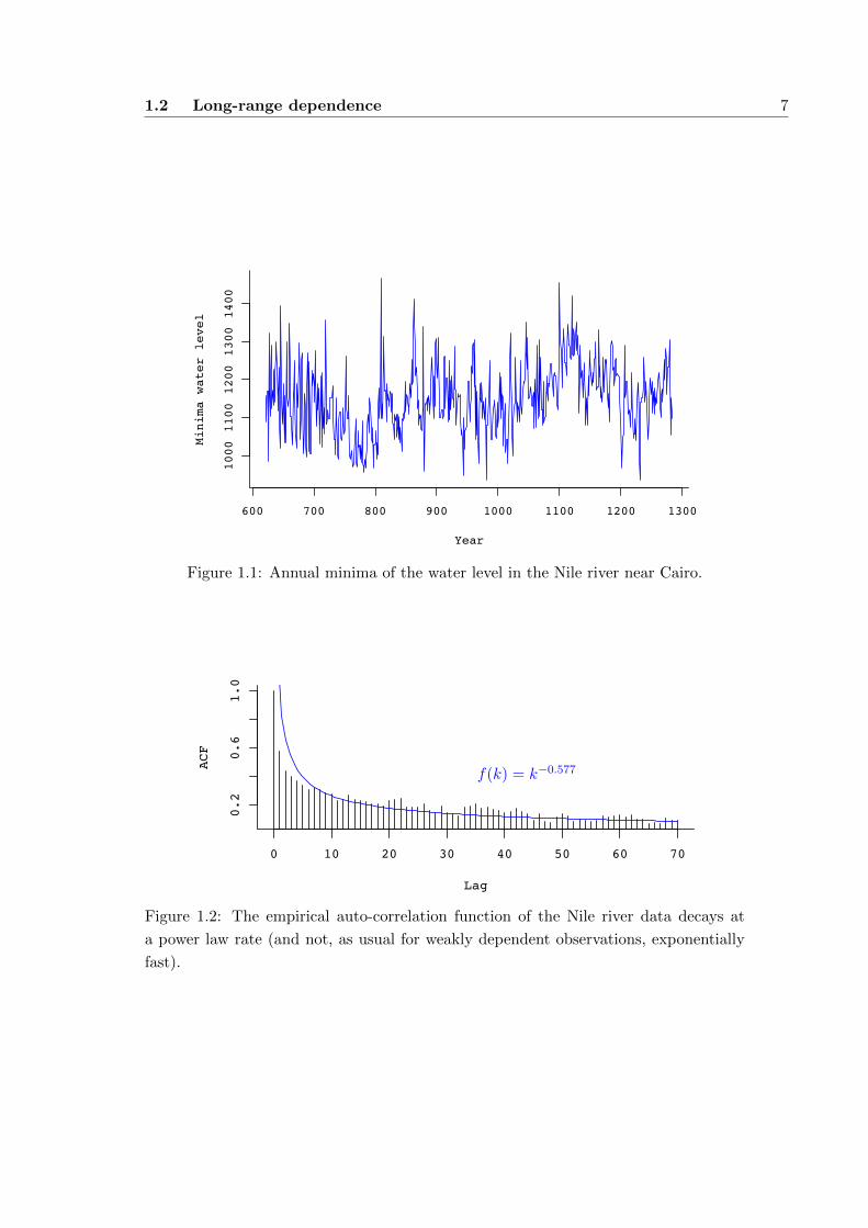
We consider a classical historic example. In the 1950s, the British hydrologist Harold
Hurst was interested in dam design and therefore in the long-term storage capacity of
reservoirs. He studied the water flow in the Nile river (Hurst, 1951, 1955) and analysed
a remarkable ancient data set, the annual minima of the water level in the Nile river at
a gauge near Cairo between 622 and 1281, which is displayed in Figure 1.1. These data
behave strange, and in fact, this can be explained by LRD: The auto-covariance func-
tion of the data, shown in Figure 1.2, decays at a power law rate. This long memory
causes the wave-like shape of the time series: Extreme large observations entail other
large observations, and extreme small observations entail other small ones. For more
statistical evidence for this type of LRD in the Nile river data, see Beran (1994, p. 21).
As indicated by the phrase “this type of LRD”, it is not mandatory to define LRD
by the decay of correlations. It has the advantage to be a handy concept, but various
other points of view are also reasonable when talking about LRD, since it is linked with
non-stationary processes, ergodic theory, self-similar processes and fractionally differ-
enced processes. Samorodnitsky (2007) discusses these concepts (and by the way notes
that in literature there can be found eleven different definitions of what exactly LRD is).
Even though it causes strange and unusual behaviour, LRD has found a very large
number of applications. Some, collected at random, are:
• Finance. Volatilities, roughly defined as the diffusion of price fluctuations, are
LRD processes (Breidt, Crato and de Lima, 1998), and there is some evidence of
a low LRD in stock market prices (Willinger, Taqqu and Teverovsky, 1999).
There is little or no evidence for the presence of LRD in the big capital markets
of the G-7 countries and in international stock market returns (Cheung and Lai,
1995), but long memory has been detected for example in the smaller Greek stock
market (Barkoulas, Baum and Travlos, 1996).
Baillie (1996) provides a survey of the major econometric work on LRD, fractional
integration and their application in economics, including an extensive list of ref-
erences. He finds substatial evidence that LRD processes describe well inflation
rates.
Cheung (1993) finds evidence for LRD in some exchange rates.
In financial time series, observations are often uncorrelated, but the auto-correlation
of their squares may be not summable; Beran (2010, p. 28) lists some references.
1.2 Long-range dependence 7
Year
Mini
ma w
ater
lev
el
600 700 800 900 1000 1100 1200 1300
1000
1100
1200
1300
1400
Figure 1.1: Annual minima of the water level in the Nile river near Cairo.
f(k) = k−0.577
0 10 20 30 40 50 60 70
0.2
0.6
1.0
Lag
ACF
Figure 1.2: The empirical auto-correlation function of the Nile river data decays at
a power law rate (and not, as usual for weakly dependent observations, exponentially
fast).

8 What it is about
When large orders are split up and executed incrementally and the size of such
large orders follows a power law, then the signs of executed orders (to buy or
to sell) have auto-correlations that exhibit a power-law decay (Lillo, Mike and
Farmer, 2005).
• Network engineering. As the internet, an enormously complicated connection
of networks, expands fastly and as the amount of memory-intensive content like
videos increases, it is crucial to maintain a high networking performance. Here,
LRD has a considerable impact on queueing performance and is a characteristic
for some problems in data traffic engineering (Erramilli, Narayan and Willinger,
1996).
Many papers focus on long memory in network data and on its impact on the
networking performance, and indeed, LRD is an omnipresent property of data
traffic both in local area networks and in wide area networks. Evidence for LRD
can be found in many measurements of internet traffic like traffic load and packet
arrival times; for examples and references see Li and Mills (1998) or Karagiannis,
Faloutsos and Riedi (2002).
LRD in network traffic can be explained by renewal processes that exhibit heavy-
tailed interarrival distributions (Levy and Taqqu, 2000).
A short overview about detection of LRD in internet traffic beside complex scaling
and multifractal behaviour, periodicity, noise and trends is provided by Karagian-
nis, Molle and Faloutsos (2004), and Cappe et al. (2002) give a tutorial about
statistical models for analyzing long-range dependence in network traffic data.
Taqqu, Willinger and Sherman (1997) and Willinger et al. (1997) demonstrated
that the superposition of many ON/OFF sources with strictly alternating ON-
and OFF-periods and whose ON-periods or OFF-periods exhibit high variabil-
ity or infinite variance can produce aggregate network traffic that exhibits self-
similarity or LRD. This provides a physical explanation for the observed self-
similar traffic patterns in high-speed network traffic.
• Physics. Particle diffusion in an electric current across two coupled supercon-
ductors shows LRD (Geisel, Nierwetberg and Zacherl, 1985), and the dynamics
of aggregates of amphiphilic (both water-loving and fat-loving) molecules as well
(Ott et al., 1990).
• Biology. Long-range power law correlation has been found in some DNA se-
quences and it is an issue in computational molecular biology (Peng et al., 1992,
1994; Buldyrev et al., 1995).
LRD can be found in human coordination: If people are asked to sychronizing
a movement (a fingertapping e.g.) to a periodic signal, the errors exhibit long
memory, as Chen, Ding and Kelso (1997) have observed. They conjecture that
this origins in random noise and sensory delay in the nervous system.

1.3 Fractional Brownian motion and fractional Gaussian noise 9
• Climate. LRD appears in surface air temperature: It can be detected in global
data from the Intergovernmental Panel on Climate Change (Smith, 1993), and
Caballero, Jewson and Brix (2002) show that the auto-covariance structure of
observed temperature data can be reproduced by fractionally integrated time
series; they explain the observed long memory by aggregation of several short-
memory effects.
Moreover, ground based observations and satellite measurements reveal that ozone
and temperature fluctuations in short time intervals are correlated to those in
large time intervals in a power law style (Varotsos and Kirk-Davidoff, 2006).
• And else. Many time series in political analysis (concerning variables like pres-
idential approval or the monthly index of consumer sentiment) show LRD char-
acteristics, as Lebo, Walker and Clarke (2000) write. They point out that many
time series in political science are aggregated measures of single responses and
that this aggregating of heterogenous individual-level information produces frac-
tional dynamics.
Long-range correlations appear also in human written language, beyond the short-
range correlations which result from syntactic rules and apparently regardless of
languages: They have been detected in Shakespeare’s plays (Montemurro and
Pury, 2002) and in novels in Korean langugage whose syntax differns strongly
from the English one (Bhan et al., 2006).
A short overview about probabilistic foundations and statistical models for LRD
data including extensive references is given by Beran (2010), while, even though older,
Beran (1994) provides a more detailed survey. Taqqu, Teverovsky and Willinger (1995)
and Taqqu and Teverovsky (1998) analyse a handful estimators that quantify the in-
tensity of LRD in time series. Details on the models used for simulations in this work
are presented in Section 1.3.
1.3 Two important LRD processes: fractional Brownian
motion and fractional Gaussian noise
Now I will introduce two prominent and important examples of LRD time series, the
fractional Brownian motion (fBm) and its incremental process, the fractional Gaussian
noise (fGn). To this end, we need some definitions. LRD processes are closely connected
with self-similar processes, where a change of the time scale is equivalent to a change
in the state space.

10 What it is about
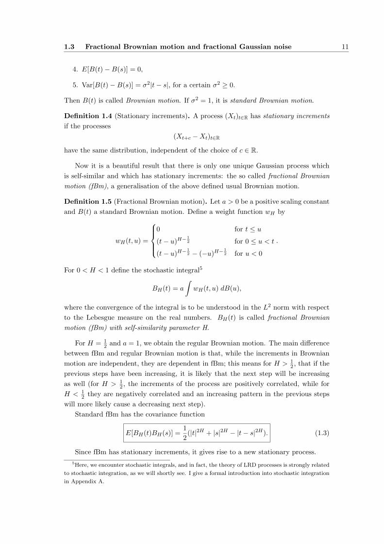
Definition 1.2 (Self-similar). A continuous time process (Xt)t∈R is called self-similar2
with index H, if for all a > 0 and any integer k ≥ 1
(Xat1 , Xat2 , . . . , Xatk)D= (aHXt1 , a
HXt2 , . . . , aHXtk), (1.2)
in other words if the finite-dimensional distributions of (Xat)t∈R are identical to the
finite-dimensional distributions of (aHXt)t∈R.
As a consequence, typical sample paths of self-similar processes look qualitatively
the same, irrespective of the time interval of observation, that is the picture stays
structually the same, irrespective of if we look from distance or if we get closer.
The notion of self-similarity was introduced into statistics by Mandelbrot and van
Ness (1968) and Mandelbrot and Wallis (1969a,b); Lamperti (1962) and Taqqu (1975)
showed that self-similar processes occur naturally as limits of partial sums of stationary
random variables, see also Pipiras and Taqqu (2011, Chap. 1.7). In nature, a fascinat-
ing richness of deterministic self-similarities can be observed, for example at leaves,
montains and waves. In 1827, the scottish botanist Robert Brown (1773–1858) exam-
ined pollen particles suspended in water under a microscope and observed an erratic
motion3. To his honour4, the most simple and important self-similar process is called
Brownian motion. Its definition is the following, see e.g. Beran (1994).
Definition 1.3 (Brownian motion). Let B(t) be a stochastic process with continuous
sample paths and such that
1. B(t) is a Gaussian process,
2. B(0) = 0 almost surely,
3. B(t) has independent increments, i.e. for all t, s > 0 and 0 ≤ u ≤ min(t, s),
B(t)−B(s) is independent of B(u),
2Because this definition refers to equality in distribution and the property can not be spotted at a
single path of Xt, one should say “statistical self-similar”, and to be entirely correct, one should say
“statistical self-affine”, because H does not need to be 1, so that the scaling in time and space to obtain
equality in distribution may be different.3Some scientists have doubted that Brown’s microscopes were sufficient to observe these movements
(D. H. Deutsch: Did Robert Brown Observe Brownian Motion: Probably Not, Scientific American,
1991, 265, p. 20), but already in the same year, a British microscopist has repeated Brown’s experiment
(B. J. Ford: Robert Brown, Brownian Movement, and Teethmarks on the Hatbrim, The Microscope,
1991, 39, p. 161–171) and finally a recent study which analysed Brown’s original observations under
historical, botanical, microscopical and physical aspects could resolve all doubt (P. Pearle, B. Collett,
K. Bart, D. Bilderback, D. Newman, S. Samuels: What Brown saw and you can too. Am. J. Phys.,
2010, 78, p. 1278–1289).4By the way, neither did Brown provide an explanation for the observed random motion, nor was he
the first to discover it: The Dutch biologist and chemist Jan Ingenhousz (1730–1799) described in 1785
an irregular movement of coal dust on the surface of alcohol, thus he, not Brown, is the true discoverer
of what came to be known as Brownian motion (P. W. van der Pas: The discovery of the Brownian
motion, Scientiarum Historia, 1971, 13, p. 27–35).
1.3 Fractional Brownian motion and fractional Gaussian noise 11
4. E[B(t)−B(s)] = 0,
5. Var[B(t)−B(s)] = σ2|t− s|, for a certain σ2 ≥ 0.
Then B(t) is called Brownian motion. If σ2 = 1, it is standard Brownian motion.
Definition 1.4 (Stationary increments). A process (Xt)t∈R has stationary increments
if the processes
(Xt+c −Xt)t∈R
have the same distribution, independent of the choice of c ∈ R.
Now it is a beautiful result that there is only one unique Gaussian process which
is self-similar and which has stationary increments: the so called fractional Brownian
motion (fBm), a generalisation of the above defined usual Brownian motion.
Definition 1.5 (Fractional Brownian motion). Let a > 0 be a positive scaling constant
and B(t) a standard Brownian motion. Define a weight function wH by
wH(t, u) =
0 for t ≤ u
(t− u)H−12 for 0 ≤ u < t
(t− u)H−12 − (−u)H−
12 for u < 0
.
For 0 < H < 1 define the stochastic integral5
BH(t) = a
∫wH(t, u) dB(u),
where the convergence of the integral is to be understood in the L2 norm with respect
to the Lebesgue measure on the real numbers. BH(t) is called fractional Brownian
motion (fBm) with self-similarity parameter H.
For H = 12 and a = 1, we obtain the regular Brownian motion. The main difference
between fBm and regular Brownian motion is that, while the increments in Brownian
motion are independent, they are dependent in fBm; this means for H > 12 , that if the
previous steps have been increasing, it is likely that the next step will be increasing
as well (for H > 12 , the increments of the process are positively correlated, while for
H < 12 they are negatively correlated and an increasing pattern in the previous steps
will more likely cause a decreasing next step).
Standard fBm has the covariance function
E[BH(t)BH(s)] =1
2(|t|2H + |s|2H − |t− s|2H). (1.3)
Since fBm has stationary increments, it gives rise to a new stationary process.
5Here, we encounter stochastic integrals, and in fact, the theory of LRD processes is strongly related
to stochastic integration, as we will shortly see. I give a formal introduction into stochastic integration
in Appendix A.

12 What it is about
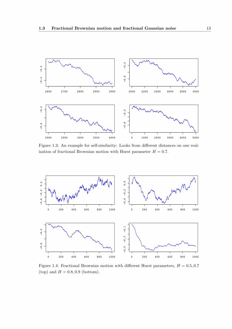
Definition 1.6 (Fractional Gaussian noise). Let BH(t) be a fBm, as in Definition 1.5.
Its incremental process
ξk = BH(k + 1)−BH(k), k ∈ Z,
is called fractional Gaussian noise (fGn).
Standard fGn has the auto-covariance function
γk =1
2
(|k + 1|2H − 2|k|2H + |k − 1|2H
), k ∈ Z, (1.4)
and for H 6= 12 it holds
γk ∼ H(2H − 1)k−(2−2H) =(1−D)(2−D)
2k−D, (1.5)
see, e.g., Samorodnitsky and Taqqu (1994). (1.5) shows the above mentioned link
between self-similarity and LRD: Fractional Gaussian noise, the incremet process of
the only self-similar Gaussian process, is an LRD process, compare to (1.1). If H = 12 ,
fGn is regular white noise, and since it is Gaussian, it is i.i.d..
1.3 Fractional Brownian motion and fractional Gaussian noise 13
2600 2700 2800 2900 3000
-0.3
-0.2
2000 2200 2400 2600 2800 3000
-0.4
-0.2
2000 2500 3000 3500 4000
-0.6
-0.2
0 1000 2000 3000 4000 5000
-0.8
-0.2
Figure 1.3: An example for self-similarity: Looks from different distances on one real-
ization of fractional Brownian motion with Hurst parameter H = 0.7.
0 200 400 600 800 1000
-0.6
-0.2
0.2
0 200 400 600 800 1000
-0.4
-0.2
0.0
0 200 400 600 800 1000
-0.6
-0.2
0 200 400 600 800 1000
-0.5
-0.3
-0.1
Figure 1.4: Fractional Brownian motion with different Hurst parameters, H = 0.5, 0.7
(top) and H = 0.8, 0.9 (bottom).
14 What it is about
f(k) = (1−D)(2−D)2 k−D = 0.28k−0.6
0 200 400 600 800 1000
-3
-1
01
23
0 200 400 600 800 1000
-3
-1
12
3
0 200 400 600 800 1000
-3
-2
-1
01
2
0 5 10 15 20 25 30
0.1
0.2
0.3
0.4
Lag
ACF
Figure 1.5: Fractional Gaussian noise with Hurst parameters H = 0.5 (top left, i.e.
white noise), H = 0.7 (top right) and H = 0.9 (bottom left). At the bottom right, the
empirical auto-correlation function of fGn with Hurst parameter H = 0.7 (i.e. D = 0.6)
is shown.
0.0 0.2 0.4 0.6 0.8 1.0
0.0
0.4
0.8
D
D_G
0.5 0.6 0.7 0.8 0.9 1.0
0.5
0.7
0.9
H
H_G
m=1m=2m=3m=4
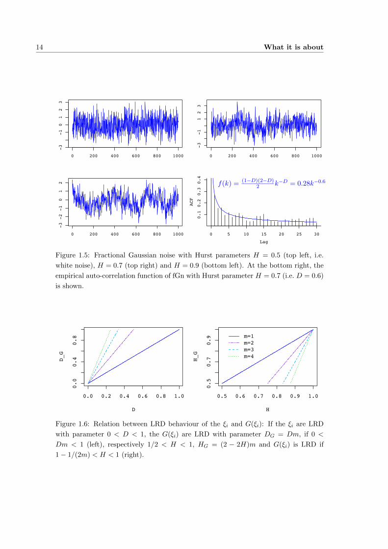
Figure 1.6: Relation between LRD behaviour of the ξi and G(ξi): If the ξi are LRD
with parameter 0 < D < 1, the G(ξi) are LRD with parameter DG = Dm, if 0 <
Dm < 1 (left), respectively 1/2 < H < 1, HG = (2 − 2H)m and G(ξi) is LRD if
1− 1/(2m) < H < 1 (right).
1.4 Hermite polynomials 15
1.4 Hermite polynomials
When tackling statistics of LRD observations, it has turned out to be useful to expand
the statistic whose asymptotic behaviour one is interested in in so called Hermite poly-
nomials. Since different definitions are used in different books and articles, it is not
amiss to give a review here.
1.4.1 Definition and basic properties
Definition 1.7 (Hermite polynomials). The functions
Hk(x) = (−1)kex2/2 d
k
dxke−x
2/2, k = 0, 1, 2, . . .
are called Hermite polynomials.
The first few are given by
H0(x) = 1
H1(x) = x
H2(x) = x2 − 1
H3(x) = x3 − 3x
H4(x) = x4 − 6x2 + 3.
Hermite polynomials have many interesting and important properties:
• Hk(x) is a polynom (what else when it is called polynom?) of degree k with
leading coefficient 1.
• Hk(x), k = 0, 1, 2, . . . form an orthogonal basis of the Hilbert space L2(R,N ), the
space of real functions which are square-integrable with respect to the N (0, 1)
density function:
〈Hi, Hj〉N = (2π)−1/2
∫ ∞−∞
Hi(x)Hj(x)e−x2/2 dx =
0 i 6= j
i! i = j
For a simple proof, see e.g. Pipiras and Taqqu (2011, Chap. 3.1).
• The Hermite polynomials in L2(Rd,N ), the Hilbert space of square-integrable
functions on Rd with respect to the independent d-dimensional standard normal
measure, can simply be defined as the product of d one-dimensional Hermite
polynomials: Hk1,...,kd(x1, . . . , xd) = Hk1(x1) · . . . ·Hkd(xd).
• Hk+1(x) = xHk(x)− kHk−1(x)
• ddxHk(x) = kHk−1(x)

16 What it is about
• One may admit an additional parameter ρ and define the Hermite polynomials
by
Hk(x, ρ) = (−ρ)kex2/2ρ d
k
dxke−x
2/2ρ, k = 0, 1, 2, . . . ,
the first few are
H0(x, ρ) = 1
H1(x, ρ) = x
H2(x, ρ) = x2 − ρ
H3(x, ρ) = x3 − 3ρx
H4(x, ρ) = x4 − 6ρx2 + 3ρ2.
• There are many further identities involving Hermite polynomials; for an impres-
sive overview and some references, see Weisstein (2010).
The definition above is sometimes called the “probabilists’ definition” because of
the normal weight. Widely spread is as well the “physicists’ definition”
H(phy)k (x) = (−1)kex
2 dk
dxke−x
2,
which defines an orthogonal basis of L2(R) with respect to the weight e−x2. Both
definitions are related by H(phy)k (x) = 2k/2Hk(
√2x).
Often Hermite functions
hk(x) = H(phy)k (x)e−x
2/2
or normalized Hermite functions
hk(x) =1√
2kk!√πH
(phy)k (x)e−x
2/2
are considered. The hk, k = 0, 1, . . . form an orthonormal basis for L2(R, λ).
1.4.2 Relation to LRD
We will now outline the important role of Hermite polynomials in the context of LRD.
Let ξ1, . . . , ξN be Gaussian random variables with mean 0, variance 1 and covariances
(1.1); such variables exhibit long memory. Now consider the partial sum
SN =
N∑i=1
h(ξi),
where h is a centralized function in L2(R,N ): h is measurable with Eh(ξi) = 0 and
Eh2(ξi) <∞. We will see that the asymptotic behaviour of this sum is closely associ-
ated with the asymptotic behaviour of the Hermite polynomials Hk(ξi).
1.4 Hermite polynomials 17
For a start we assume that h itself is already a Hermite polynomial Hk. Now the
growth of the partial sum is essentially governed by the fundamental property6
Cov [Hm(ξi), Hn(ξj)] =
m! (Cov [ξi, ξj ])m m = n
0 otherwise, (1.6)
and we have
Var
[N∑i=1
Hk(ξi)
]=
N∑i=1
Var[Hk(ξi)] + 2N−1∑j=1
(N − j) Cov [Hk(ξ1), Hk(ξ1+j)]
= Nk! + 2k!N−1∑j=1
(N − j)γkj
= Nk! + 2k!N−1∑j=1
(N − j)j−DkL(j)k. (1.7)
Now it is obvious that the limiting behaviour depends on the size of Dk. If Dk > 1,
the sum is O(N) and the variance of the partial sum grows asymptotically like N , just
like in the weak dependent or in the independent case. But if Dk < 1, the situation is
quite different: Like in (B.6) we find the asymptotic equivalence
Var
[N∑i=1
Hk(ξi)
]∼ Nk! +
2k!
(1−Dk)(2−Dk)N2−DkL(N)k
= N2−DkL(N)kk!
(1
N1−DkL(N)k+
2
(1−Dk)(2−Dk)
)∼ N2−DkL(N)kk!
2
(1−Dk)(2−Dk).
So we see the extraordinary property of long memory statistics: The size of the
LRD parameter D and the degree of the Hermite polynomial k determine the growth
of the variance of the partial sum – for Dk > 1 we observe usual SRD behaviour, while
for Dk < 1 we observe a faster rate of growth (wich also can be taken as a definition
of LRD7):
Var
[N∑i=1
Hk(ξi)
]∼
Nk!CSRD, if Dk > 1,
N2−DkL(N)k 2k!(1−Dk)(2−Dk) , if Dk < 1,
(1.8)
6This follows from the diagram formula. With this formula one can compute expectations and
cumulants of finite families of random variables, for example expectations of Hermite polynomials of
Gaussian variables, but it is not a walk in the park. I will introduce a special version of the formula
and give some examples in Section 2.5. Without going too much into theoretical details, one can see
for example Beran (1994, eq. (3.18)) or Simon (1974, Th. 1.3), where the statement is proved for Wick
powers, random variables with special properties; Hermite polynomials – in the probabilists’ definition
with respect to the normal density measure – are a special case of Wick powers. Results on Wick
powers can also be found in Major (1981a, p. 9). A general introduction to the diagram formula is
given by Surgailis (2003).7This is the so called LRD in the sense of Allen (Pipiras and Taqqu, 2011, Chap. 1.1).

18 What it is about
where CSRD is a constant. (Moreover, Dk influences the limit distribution in a broader
sense, as we will shortly see.) We will focus on the second case, because here the
variance of the partial sum grows faster than with the usual rate N , and this is the
case where also the limit distribution of the partial sum can be non-normal. The case
Dk = 1 is special; here the usual central limit theorem holds, but the norming factor
may be different than the usual√N , see e.g. the discussion of Theorem 8.3 in Major
(1981a), the remark in Dobrushin and Major (1979, p. 30) or Breuer and Major (1983,
p. 428).
Now we turn to a more generel kernel h(x). We represent it by its Hermite expansion
h(x) =∑∞
k=1 ak/k! Hk(x) (the equality is to be understood as convergence in L2) with
coefficients
ak := 〈h,Hk〉N = (2π)−1/2
∫ ∞−∞
h(x)Hk(x)e−x2/2 dx.
Now the partial sum is
Var
[N∑i=1
h(ξi)
]= Var
[ ∞∑k=1
akk!
N∑i=1
Hk(ξi)
]
=
∞∑k=1
a2k
k!2Var
[N∑i=1
Hk(ξi)
]+
∞∑k 6=l
N∑i=1
N∑j=1
akalk! l!
Cov [Hk(ξi), Hl(ξj)]
=∞∑k=1
a2k
k!2Var
[N∑i=1
Hk(ξi)
]
because of the orthogonality of the Hl, Hk. Now let m be the Hermite rank of h(x), the
smallest index among those k ∈ N with ak 6= 0. The term with the belonging coefficient
am dominates all others, because for an arbitrary k > m we have by (1.8)
a2k Var
[∑Nj=1Hk(ξj)
]a2m Var
[∑Nj=1Hm(ξj)
] ∼ a2kl!(1−Dm)(2−Dm)
a2mm!(1−Dl)(2−Dl)
N−D(k−m)L(N)k−m → 0
as N →∞. Thus
Var
N∑j=1
h(ξj)
∼ a2m
m!2
Nm!CSRD, if Dm > 1,
N2−DmLm(N)cm, if Dm < 1(1.9)
with CSRD, cm ∈ R (to be more precise cm = 2m!(1−Dm)(2−Dm)).
Finding the limit distribution of SN is challenging. What makes functionals of
LRD observations tricky is that they may have a non-normal limit. Although the most
interesting cases, thankfully, follow a normal distribution, almost all functionals of long-
range dependent observations have a limit which is neither normal nor easy (or possible)
to write down in a closed form. Dobrushin and Major (1979) and, independently, Taqqu
(1979) have derived a general representation for the limit: It can be expressed in terms
of so called multiple Wiener-Ito integrals. In Appendix A, I explain the idea behind

1.4 Hermite polynomials 19
these objects. We now quote a result from Dobrushin and Major (1979), which holds
in greater generality, namely for processes, see also Major (1981b).
Theorem 1.1 (Non-central limit theorem for LRD processes). Let Dm < 1. Then as
N →∞ d−1N
btNc∑i=1
h(ξi)
t∈[0,1]
D−→amm!
Zm(t)t∈[0,1]
(1.10)
with
Zm(t) = K−m/2c−1/2m
∫ ′Rm
eit∑mj=1 xj − 1
i∑m
j=1 xj
m∏j=1
|xj |(D−1)/2
dW (x1) . . . dW (xm)
(1.11)
d2N = d2
N (m) = cmN2−DmLm(N), (1.12)
where i is the imaginary unit and
K =
∫Reix|x|D−1 dx = 2Γ(D) cos(Dπ/2),
cm =2m!
(1−Dm)(2−Dm).
Formula (1.11) denotes the multiple Wiener-Ito integral with respect to the random
spectral measure W of the white-noise process, where∫ ′
means that the domain of
integration excludes the hyperdiagonals xi = ±xj , i 6= j, see also Dehling and Taqqu
(1989, p. 1769). The constant of proportionality cm ensures that E[Zm(1)]2 = 1. Taqqu
(1979) or Pipiras and Taqqu (2011, Chap. 3.2) give another representation.
Technical remark. The limit is – as here – often denoted as Zm(t). However, one has to pay atten-
tion, because whether a special Zm(t) is normalized (so that E[Zm(1)]2 = 1) or not, differs from article
to article (even when they are written by the same author).
For instance in the case of Hermite rank m = 1, the limit is
a1Z1(t) = a1
(1
2Γ(D) cos(Dπ/2)
)1/2((1−D)(2−D)
2
)1/2 ∫ eitx − 1
ix|x|(D−1)/2 dW (x)
= a1
(Γ(3−D) sin(Dπ/2)
2π
)1/2 ∫ eitx − 1
ix|x|(D−1)/2 dW (x)
and with D = 2− 2H
= a1
(HΓ(2H) sin(πH)
π
)1/2 ∫ eitx − 1
ix|x|−(H−1/2) dW (x)
= a1BH(t)
20 What it is about
which is a fractional Brownian motion at time t. The first equality can be shown by
Euler’s reflection formula for the Gamma function, Γ(z)Γ(1 − z) = π/ sin(πz), and a
trigonometric double-angle identitiy; the last equality is proved by Taqqu (2003, Prop.
9.2). So we receive
N−1+D2 L(N)−1/2
btNc∑i=1
h(ξi)D−→ a1
(2
2H(2H − 1)
)1/2
BH(t) (1.13)
= a1
(2
(1−D)(2−D)
)1/2
B1−D/2(t),
which has been proven directly by Taqqu (1975, Cor. 5.1).
We have just seen how the Hermite rank of a function h influences the variance of the
partial sum SN =∑N
i=1 h(ξi). If the underlying Gaussian process (ξ)i≥1 is LRD with
parameter D ∈ (0, 1), the partial sum SN inherits LRD-type behaviour if Dm ∈ (0, 1),
where m is the Hermite rank of h. This rate of growth, N2−Dm instead of N , is closely
related with the definition of LRD as given in Definition 1.1, see the discussion by
Pipiras and Taqqu (2011, Chap. 1.1), and in fact it can be taken as a definition for
LRD. But here, we work with Definition 1.1, so to conclude this chapter, we will now
show under which conditions a stationary Gaussian process (ξi)i≥1 passes its LRD, in
the sense of Definition 1.1, on to the transformed process (Xi)i≥1, Xi = G(ξi).
Let ξ, η be two standard normal random variables and G1, G2 ∈ L2(R,N ) two
functions. We expand G1 and G2 in Hermite polynomials
G1(x) =∞∑k=0
a1,k
k!Hk(x) G2(x) =
∞∑l=0
a2,l
l!Hl(x)
where ai,k = E[Gi(ξ)Hk(ξ)] is the associated k-th Hermite coefficient. With these
expansions, (1.6) yields
Cov [G1(ξ), G2(η)] = E [G1(ξ)G2(η)]− E [G1(ξ)]E [G2(η)]
=
∞∑k=0
∞∑l=0
a1,k
k!
a2,l
l!E [Hk(ξ)Hl(η)]− E [G1(ξ)]E [G2(η)]
=∞∑k=0
a1,k
k!
a2,k
k!k! (E[ξη])k − E [G1(ξ)H0(ξ)]E [G2(η)H0(η)]
=∞∑k=0
a1,k
k!
a2,k
k!k! (E[ξη])k − a1,0a2,0
=∞∑k=1
a1,k
k!
a2,k
k!k! (E[ξη])k .
We have just proved the following
1.4 Hermite polynomials 21
Proposition 1.2. Consider a stationary Gaussian process (ξi)i≥1 with mean 0 and
variance 1 and auto-covariance as in (1.1). Let G ∈ L2(R,N ) have Hermite rank m.
Then the process (Xi)i≥1 = (G(ξi))i≥1 has auto-covariances
γG(k) = Cov[Xi, Xi+k] = Cov[G(ξi), G(ξi+k)]
=∞∑p=1
a2p
p!(E[ξiξi+k])
p ,
and the first term in this expansion dominates the others, such that
γG(k) ∼ a2m
m!
(L(k)k−D
)m,
thus if 0 < Dm < 1, (G(ξi))i≥1 is LRD in the sense of Definition 1.1 with LRD
parameter DG = Dm and slowly varying function LG(k) = a2m/m!Lm(k).
As a consequence, (ξi)i≥1 may be LRD, but (G(ξi))i≥1, e.g. (ξ2i )i≥1 may be not.
Figure 1.6 shows the relation between the LRD parameter D of the underlying ξi’s and
the LRD parameter DG of the transformed G(ξi)’s.

22 What it is about
Chapter 2
The asymptotic behaviour of
X − Y
Before we investigate change-point tests, we consider the two-sample Gauß test which
is traditionally used to detect a difference in the location of two samples of normal dis-
tributed observations. This test follows as a special case from the ”difference-of-means“
change-point test which we will discuss later (see section 3.4.2) – it is nothing else than
the change-point test applied in a situation with a known change-point and with only
Gaussian data –, but this example illustrates the impact of LRD on statistical proce-
dures, the impact of persistent correlations, and as a basic and direct approach, it may
lead to an intuitive understanding of the subject.
So suppose we have observed some data and we suspect that after the m-th obser-
vation there has been a change in the mean:
X1, X2, . . . , Xm ∼ N (µ1, σ2) (2.1)
Xm+1, Xm+2, . . . , Xm+n ∼ N (µ2, σ2)
We want to find out if there really has been a change or not: We wish to test the
nullhypothesis H : µ1 = µ2 against the alternative A : µ1 6= µ2. A natural idea to do
this is to compare the means of both samples. To be in line with standard notation,
we call the second sample the Y -sample (Yk := Xm+k) and consider the data
X1, X2, . . . , Xm ∼ N (µ1, σ2)
Y1, Y2, . . . , Yn ∼ N (µ2, σ2).
In the i.i.d. case and with unknown variance σ2, a common test for the problem
(H,A) is the t-test which is based on the difference of the means
T =
√mn
m+ n
X − YsX,Y

24 The asymptotic behaviour of X − Y
with the weighted variance
s2X,Y =
(m− 1)s2x + (n− 1)s2
y
m+ n− 2,
where s2x and s2
y are the empirical variances of the X- and the Y -sample. From intro-
ductory mathematical statistics we know that under H, T ∼ tm+n−2, so we reject H
on a significance level of α, if |T | > tα/2, n+m−2, where tα,q is the upper α-quantile of
Student’s t-distribution with q degrees of freedom.
We will examine the LRD case with observations from a stationary Gaussian pro-
cess (Xi)i≥1 with mean 0, variance 1 and auto-covariance (1.1). One should expect
that X − Y shows a different behaviour in this case, since long memory requires a
stronger normalization factor and often leads to non-normal limit distributions. We
shall see that this intuition is right. But first, we need some preliminaries to handle
the covariance structure for it is given as an asymptotic equivalence and it contains a
slowly varying function.
Finally, we will estimate the variance of X − Y in this chapter. To this end, we will
propose an estimator for the variance of the mean XN =∑N
i=1Xi and an estimator for
the auto-covariances γk = Cov[Xi, Xi+k] in a sample of N observations X1, . . . , XN , as
N tends to ∞. We base our estimator for the variance of X − Y on these two methods
and demonstrate that all these estimators are asymptotically unbiased.
2.1 Asymptotic equivalence and slowly varying functions
Definition 2.1 (Asymptotic equivalence). Two real functions f and g are called asymp-
totically equivalent as x→∞, written as f ∼ g, if
limx→∞
f(x)
g(x)= 1.
Asymptotically equivalent functions have the same limit, if it exists, and the same
growth behaviour as x increases.
Definition 2.2 (Slowly varying function). A real function L : (0,∞)→ (0,∞) is called
slowly varying (at infinity) if for all a > 0
limx→∞
L(ax)
L(x)= 1.
Any function with limx→∞ L(x) = b ∈ (0,∞) and any power of the logarithm
L(x) = logc x, c ∈ R is slowly varying. Usual powers f(x) = xc are not slowly varying.

2.1 Asymptotic equivalence and slowly varying functions 25
Technical remark. In this work, we always consider Gaussian processes (Xi)i≥1 with mean 0, vari-
ance 1 and covariances as in (1.1), i.e. γk = Cov[Xi, Xi+k] ∼ k−DL(k), where D ∈ (0, 1) is the
parameter for the long memory and L is a slowly varying function. It makes no difference if we write
γk = k−DL(k) or γk ∼ k−DL(k), because L is not exactly specified. The asymptotic equivalence
notation makes clearer that we admit covariances whose behaviour we know only asymptotically.
L does not only model disturbance or uncertaincy, it is rather there to ensure that the covariance
matrix of the process is positive-semidefinite – what a covariance matrix has to be. γk = k−D alone
does not provide a covariance matrix because it may lead to a non-positive-semidefinite matrix, as the
following example shows:
For three observations X1, X2, X3, γk = k−D and D = 0.6 we obtain as ’covariance matrix’
Σ =(γ|k−l|
)3k,l=1
=
1 2−3/5
1 1
2−3/5 1
which has the (rounded) eigenvalues 2.782, 0.340, −0.122. But for γk = log k · k−D we obtain a true
covariance matrix
Σ =(γ|k−l|
)3k,l=1
=
1 0 log 2
23/5
0 0log 2
23/5 0 1
which now has the nice (rounded) eigenvalues 1.457, 1, 0.543.
Lemma 2.1 (Asymptotic equivalence in sums). Let (an), (bn), (αn), (βn) be sequences
of real numbers, g 6= 1 a constant and αn/βn > 0 for large n.
(i) If αn/βn → g for n→∞, then
an ∼ αn, bn ∼ βn ⇒ (an ± bn) ∼ (αn ± βn), as n→∞. (2.2)
(ii) If∑n
k=1 αk is unbounded and strictly monotonic increasing from a certain index
n0, then
an ∼ αn ⇒n∑k=1
ak ∼n∑k=1
αk, as n→∞. (2.3)
(iii) If (ak,n), (αk,n) are two sequences which depend on the indices n and k ≤ n and
satisfy
n−1∑k=1
(ak,n − ak,n−1) + an,n ∼n−1∑k=1
(αk,n − αk,n−1) + αn,n, as n→∞,
and if∑n
k=1 αk,n is unbounded and strictly monotonic increasing from a certain index
n0, thenn∑k=1
ak,n ∼n∑k=1
αk,n, as n→∞. (2.4)
Proof. (i) Let ε > 0 be given, but small enough that |g − 1| > 2ε. Choose n0 ∈ Nso big that |(an − αn)/αn| and |(bn − βn)/βn| are both smaller than ε2/(2 + g), that
|αn/βn − 1| > ε and |αn/βn − g| < 1 and that αn/βn is positive for all n ≥ n0 (we
26 The asymptotic behaviour of X − Y
can find such an index n0 because from a certain point forward, an/αn and bn/βn stay
close to 1 and αn/βn stays close to g 6= 1). Then we have for all n ≥ n0∣∣∣∣(an − bn)− (αn − βn)
αn − βn
∣∣∣∣ ≤ ||an − αn|+ |bn − βn|||αn − βn|
≤ ε2
2 + g
||αn|+ |βn|||αn − βn|
=ε2
2 + g
∣∣∣αnβn + 1− g + g∣∣∣∣∣∣αnβn − 1
∣∣∣≤ ε2
2 + g
|1 + g|+ 1
ε= ε,
and this means that an−bnαn−βn → 1, in other words (an − bn) ∼ (αn − βn). In the exact
same manner we can verify (an + bn) ∼ (αn + βn).
(ii) This is a special case of (iii), when (ak,n), (αk,n) depend only on k.
(iii) When we have two sequences of real numbers (rn) and (sn), (sn) is strictly
increasing and unbounded, and we know the convergence of the difference quotient
(rn − rn−1)/(sn − sn−1) → c, then the Stolz-Cesaro theorem (Heuser, 2003, Th. 27.3)
ensures that rn/sn → c as well. Take rn =∑n
k=1 ak,n and sn =∑n
k=1 αk,n, then
limn→∞
rn − rn−1
sn − sn−1= lim
n→∞
∑n−1k=1 (ak,n − ak,n−1) + an,n∑n−1k=1 (αk,n − αk,n−1) + αn,n
= 1,
and we receive the desired result with c = 1. A review of the proof reveals that the
Stolz-Cesaro theorem even holds if sn is not strictly monotone right from the start, but
only from a certain point on.
Example. As a counterexample where the conditions of Lemma 2.1 are not fulfilled,
consider for (i)
an = n+ 1 αn = n
bn = n βn = n+1
n;
clearly an ∼ αn and bn ∼ βn, but an − bn = 1 is not equivalent to αn − βn = − 1n . For
(ii), consider any sequence an with∑∞
k=1 ak <∞ and choose a sequence a′n < an with
a′n = o(an). Define αn := an + a′n.
Lemma 2.2 (Some properties of slowly varying functions). Consider a slowly varying
function L(x).
(i)
L(x+ a) ∼ L(x) as x→∞, for all fixed a ∈ R+ (2.5)
2.1 Asymptotic equivalence and slowly varying functions 27
(ii) If L is locally bounded (that means bounded on every compact set) and we have
γk ∼ cΓ(1−D)k
−DL(k) =: gk with D ∈ (0, 1) and a constant c, then
n∑k=1
γk ∼c
Γ(2−D)n1−DL(n). (2.6)
Proof. (i) By Karamata’s Representation Theorem (Bingham et al., 1989, Th. 1.3.1),
we can write L(x) = c(x) exp∫ x
dε(u)u du
with an arbitrary d > 0 (for instance d = 1),
c(·) mesurable and c(x)→ c ∈ (0,∞), ε(x)→ 0 as x→∞. We therefore have for large
n and an arbitrarily small ε > 0
L(x+ a)
L(x)=c(x+ a)
c(x)exp
∫ x+a
x
ε(u)
udu
≤ c(x+ a)
c(x)exp
ε
∫ x+a
x
1
udu
=c(x+ a)
c(x)
(x+ a
x
)ε→ 1
and
L(x+ a)
L(x)≥ c(x+ a)
c(x)exp
−ε∫ x+a
x
1
udu
=c(x+ a)
c(x)
(x+ a
x
)−ε→ 1,
so all in all L(x+ a)/L(x)→ 1.
(ii) Define the step function u(x) := γn for n ≤ x < n + 1. We obtain from the
Uniform Convergence Theorem (Bingham et al., 1989, Th. 1.2.1), which provides that
L(λx)/L(x) → 1 (as x → ∞) uniformly on each compact set of λ in (0,∞), that
L(x) ∼ L(n) for n ≤ x < n+ 1 and thus
u(x) ∼ cx−D
Γ(1−D)L(x).
Now we know by Karamata’s Theorem that asymptotic relations are integrable (Bing-
ham et al., 1989, Prop. 1.5.8):∫ x
at−βL(t) dt ∼ L(x)
∫ x
at−β dt ∼ x1−β
1− βL(x) as x→∞
if L(x) is locally bounded in [a,∞) and β < 1. So we can figure out the asymptotic
behaviour of∑n
k=1 γk as follows:
n∑k=1
γk =
∫ n
1u(t) dt ∼ cn1−D
(1−D)Γ(1−D)L(n)
Technical remarks. (a) As L is defined on the positive real line (0,∞), L(x − a) may formally
not be defined, but we are interested in asymptotic behaviour for x → ∞, so we can admit (fixed)
negative a in the lemma as well. If this is desired, change the variables y = x− a, and the proof covers
L(x− a) ∼ L(x) as well.
(b) As long as it is a fixed point, it is irrelevant for the asymptotic behaviour where the sum∑nk=1 γk starts. Technically we must take care that L is locally bounded on the whole domain of
summation. To ensure this, we want L to be locally bounded everywhere. For practical use this is not
a serious restriction.

28 The asymptotic behaviour of X − Y
2.2 One divided sample
At first we consider the asymptotic behaviour of the Gauß test for two samples like in
(2.1), roughly speaking one LRD time series that is cut into two samples. (Subsequent,
we will consider two independent samples which both exhibit the same LRD.)
2.2.1 Asymptotic theory
Theorem 2.3. Let (Xi)i≥1 be a stationary Gaussian process with mean 01, variance 1
and covariances
γk = Cov[Xi, Xi+k] ∼c
Γ(1−D)k−DL(k) =: gk
with c a constant, D ∈ (0, 1) and L a slowly varying function. Assume that we have a
series of N observations which is cut into two pieces:
X1, X2, . . . , Xm and Xm+1, Xm+2, . . . , Xm+n
with N = m + n. It is m = [λN ] and n = [(1 − λ)N ] for a λ ∈ (0, 1). We call the
second sample the Y -sample (Yk := Xm+k). Then for the difference of both sample
means holds √mn
(m+ n)2−DL(m+ n)
X − Yσdiff
D−→ N (0, 1) (2.7)
with
σ2diff =
2c
Γ(3−D)
(λ1−D(1− λ) + λ(1− λ)1−D − 1 + λ2−D + (1− λ)2−D)
=2c
Γ(3−D)
(λ1−D + (1− λ)1−D − 1
).
Technical remark. a) It is natural to write the limit theorem in terms of the single sample sizes
m and n, but this can be misleading, because m and n change with λ, while the above expression
erroneously suggests that only the variance σ2diff is a function of λ. Theorem 2.3 can also be written as:
ND/2L(N)−1/2 X − Yσ′diff
D−→ N (0, 1)
with
σ′2diff =
σ2diff
λ(1− λ)
=2c
Γ(3−D)
λ1−D(1− λ) + λ(1− λ)1−D − 1 + λ2−D + (1− λ)2−D
λ(1− λ)
=2c
Γ(3−D)
(λ1−D + (1− λ)1−D − 1
)λ(1− λ)
.
1In a test problem for a change-point, this corresponds to the null hypothesis that there is no change
in the mean of the data: All observations have the same mean, and we can assume that this common
mean is 0. Here, we derive the (non-degenerate) asymptotic distribution of the test statistic under this
null hypothesis. In contrast, if there is a change in the mean, i.e. if E[Xi] is the same for all i, E[Yj ] is
the same for all j, but E[Xi] 6= E[Yj ] for all i, j, then the variance blows up the mean of the statistic
as well, so the expression blows up to infinity – which gives notice of the change-point.
2.2 One divided sample 29
This variance σ′2diff has, in contrast to σ2
diff, the expected property that it has a minimum in λ = 0.5.
b) It may be advantageous to write σ2diff and σ
′2diff in the not summarized, longer form: The dif-
ference between the case of two independent samples and the case of one divided sample can easily be
seen. In the case of two independent samples, three summands of the longer representation of σ2diff and
σ′2diff are lacking.
The limit behaviour of the Gauß test statistic is a special case of the ”difference-
of-means“ change-point test which we will treat in section 3.4.2 and which has been
analyzed by Csorgo and Horvath (1997, Chap. 4.3), so we source the direct proof out to
Appendix B (the proof is substantially only calculating the variance of the test statistic,
but one has to take into account asymptotic equivalences and slowly varing functions;
even though this is laborious, it is down-to-earth analysis, so it gives a feel for LRD).
2.2.2 Simulations
We will now investigate the finite sample performance of the statistic from Theorem 2.3
in a simulation study. To this end, I have simulated 10, 000 time series of fGn2 with
Hurst parameterH (respectivelyD = 2−2H) and lengthN = 10, 50, 100, 500, 1000, 2000.
In this model, the auto-covariances are
γk ∼(
1− D
2
)(1−D)k−D
=c
Γ(1−D)k−DL(k) with L(k) ≡ 1 and c =
1
2Γ(3−D),
so Theorem 2.3 states in this situation that
T :=
√mn
(m+ n)2−DX − Yσdiff
D−→ N (0, 1)
with
σ2diff =
(λ1−D(1− λ) + λ(1− λ)1−D − 1 + λ2−D + (1− λ)2−D) .
Since T is a linear statistic of X and Y , the convergence is more than a general con-
vergence in distribution: In some sense, only the variance needs to converge to 1, the
distribution is always normal. For each of the 10, 000 time series, I have calculated
T , and based on these values, I have computed the sample variance of T . All sample
variances are pretty close to 1, no matter for which split-up or for which length of
the series. The exact results are given in Appendix D.1; the R-source code is given in
Appendix C.5. In Figure 2.1, the estimated density of T is shown, compared to the
standard normal density.
To get a feel for how the variance of X − Y behaves for different choices of λ and
H, we write
T :=
√mn
(m+ n)2−DX − Yσdiff
=
√λ(1− λ)
N−DX − Yσdiff
2See Section 1.3. I have simulated fGn via a routine in the fArma package in R which uses a fast
Fourier Transform, based on the SPLUS code presented by Beran (1994).
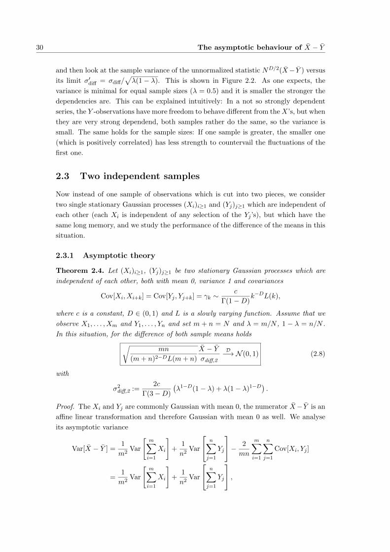
30 The asymptotic behaviour of X − Y
and then look at the sample variance of the unnormalized statistic ND/2(X− Y ) versus
its limit σ′diff = σdiff/√λ(1− λ). This is shown in Figure 2.2. As one expects, the
variance is minimal for equal sample sizes (λ = 0.5) and it is smaller the stronger the
dependencies are. This can be explained intuitively: In a not so strongly dependent
series, the Y -observations have more freedom to behave different from theX’s, but when
they are very strong dependend, both samples rather do the same, so the variance is
small. The same holds for the sample sizes: If one sample is greater, the smaller one
(which is positively correlated) has less strength to countervail the fluctuations of the
first one.
2.3 Two independent samples
Now instead of one sample of observations which is cut into two pieces, we consider
two single stationary Gaussian processes (Xi)i≥1 and (Yj)j≥1 which are independent of
each other (each Xi is independent of any selection of the Yj ’s), but which have the
same long memory, and we study the performance of the difference of the means in this
situation.
2.3.1 Asymptotic theory
Theorem 2.4. Let (Xi)i≥1, (Yj)j≥1 be two stationary Gaussian processes which are
independent of each other, both with mean 0, variance 1 and covariances
Cov[Xi, Xi+k] = Cov[Yj , Yj+k] = γk ∼c
Γ(1−D)k−DL(k),
where c is a constant, D ∈ (0, 1) and L is a slowly varying function. Assume that we
observe X1, . . . , Xm and Y1, . . . , Yn and set m + n = N and λ = m/N , 1 − λ = n/N .
In this situation, for the difference of both sample means holds√mn
(m+ n)2−DL(m+ n)
X − Yσdiff,2
D−→ N (0, 1) (2.8)
with
σ2diff,2 :=
2c
Γ(3−D)
(λ1−D(1− λ) + λ(1− λ)1−D) .
Proof. The Xi and Yj are commonly Gaussian with mean 0, the numerator X− Y is an
affine linear transformation and therefore Gaussian with mean 0 as well. We analyse
its asymptotic variance
Var[X − Y ] =1
m2Var
[m∑i=1
Xi
]+
1
n2Var
n∑j=1
Yj
− 2
mn
m∑i=1
n∑j=1
Cov[Xi, Yj ]
=1
m2Var
[m∑i=1
Xi
]+
1
n2Var
n∑j=1
Yj
,
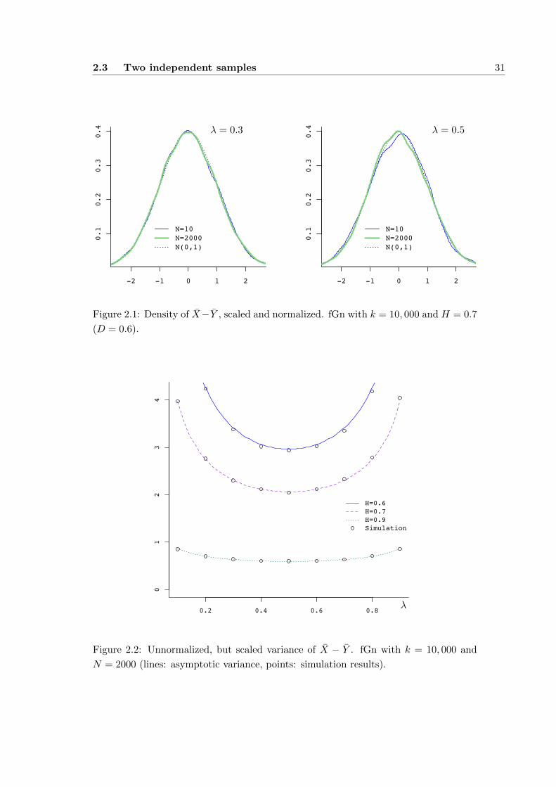
2.3 Two independent samples 31
-2 -1 0 1 2
0.1
0.2
0.3
0.4
N=10N=2000N(0,1)
-2 -1 0 1 2
0.1
0.2
0.3
0.4
N=10N=2000N(0,1)
λ = 0.3 λ = 0.5
Figure 2.1: Density of X−Y , scaled and normalized. fGn with k = 10, 000 and H = 0.7
(D = 0.6).
0.2 0.4 0.6 0.8
01
23
4
H=0.6H=0.7H=0.9Simulation
λ
Figure 2.2: Unnormalized, but scaled variance of X − Y . fGn with k = 10, 000 and
N = 2000 (lines: asymptotic variance, points: simulation results).
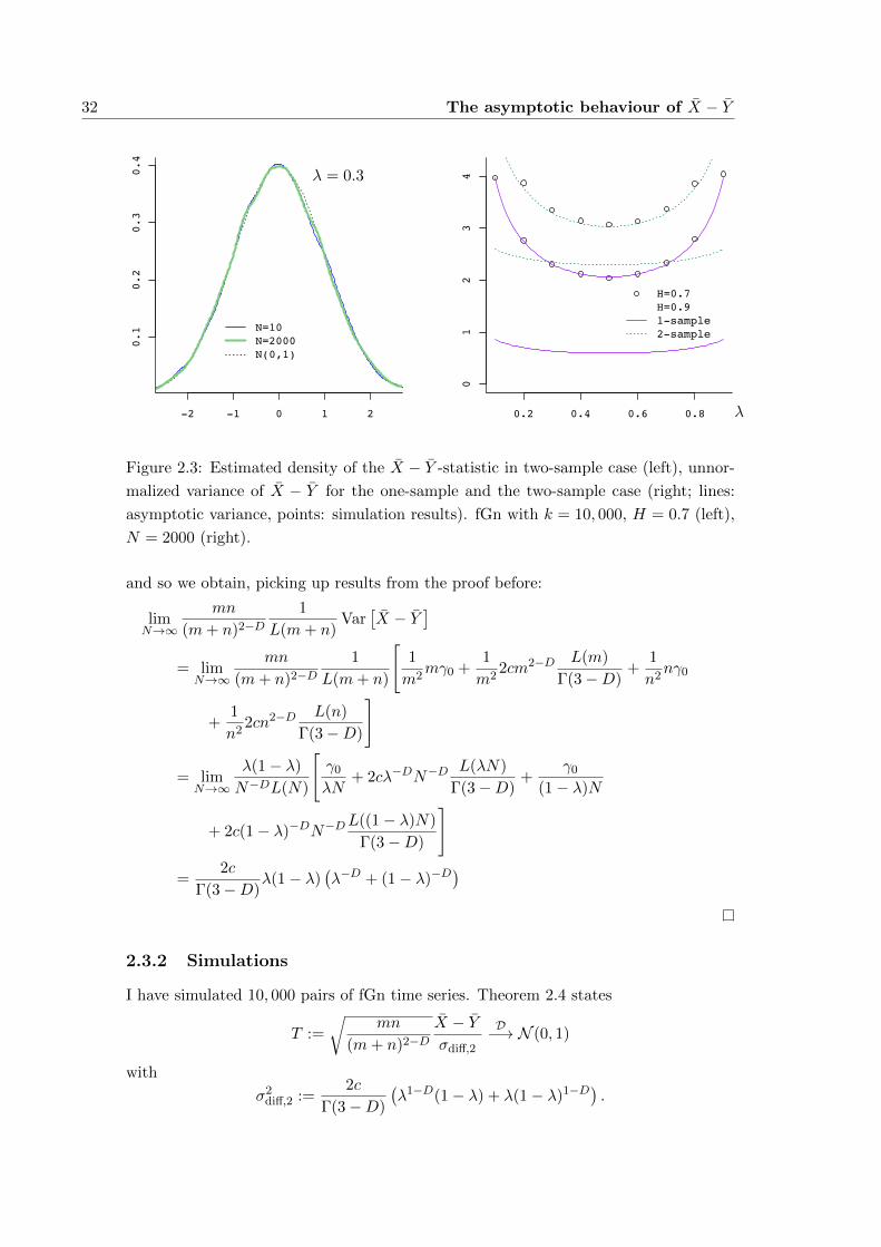
32 The asymptotic behaviour of X − Y
-2 -1 0 1 2
0.1
0.2
0.3
0.4
N=10N=2000N(0,1)
0.2 0.4 0.6 0.8
01
23
4
H=0.7H=0.91-sample2-sample
λ = 0.3
λ
Figure 2.3: Estimated density of the X − Y -statistic in two-sample case (left), unnor-
malized variance of X − Y for the one-sample and the two-sample case (right; lines:
asymptotic variance, points: simulation results). fGn with k = 10, 000, H = 0.7 (left),
N = 2000 (right).
and so we obtain, picking up results from the proof before:
limN→∞
mn
(m+ n)2−D1
L(m+ n)Var
[X − Y
]= lim
N→∞
mn
(m+ n)2−D1
L(m+ n)
[1
m2mγ0 +
1
m22cm2−D L(m)
Γ(3−D)+
1
n2nγ0
+1
n22cn2−D L(n)
Γ(3−D)
]
= limN→∞
λ(1− λ)
N−DL(N)
[γ0
λN+ 2cλ−DN−D
L(λN)
Γ(3−D)+
γ0
(1− λ)N
+ 2c(1− λ)−DN−DL((1− λ)N)
Γ(3−D)
]=
2c
Γ(3−D)λ(1− λ)
(λ−D + (1− λ)−D
)
2.3.2 Simulations
I have simulated 10, 000 pairs of fGn time series. Theorem 2.4 states
T :=
√mn
(m+ n)2−DX − Yσdiff,2
D−→ N (0, 1)
with
σ2diff,2 :=
2c
Γ(3−D)
(λ1−D(1− λ) + λ(1− λ)1−D) .

2.4 Estimating the variance of X 33
As before, all sample variances are pretty close to their asymptotic value of 1, even
for small und unequal sample sizes. The exact results are given in Appendix D.1,
while Figure 2.3 provides an overview. The R-source code of the simulation is given in
Appendix C.6.
When we plot the unnormalized variance of X − Y as in the simulations before,
we see that the variance is smaller in the one-sample case. Intuitively, this is not a
surprise: Both samples are mutually positively correlated, so they behave similar and
their difference does not fluctuate that much as in the case of two independent fGn
samples.
2.4 Estimating the variance of X
In a next step we want to estimate Var[X − Y ] in Theorem 2.3. For a start we concen-
trate on the case when N observations X1, . . . , XN are given and we want to estimate
Var[X]. (We still we consider a stationary Gaussian process (Xi)i≥1 with E[Xi] = 0,
E[X2i ] = 1 and auto-covariance function (1.1).) The problem here is that we want to
estimate the variance of a variable that we observe only one single time. So we enforce
several observations by an artifical segmenting of the observed data: We divide the
original time series X1, . . . , XN into N/r blocks of length r (for simplicity of notation
we assume that N/r is an integer) and take the sample mean over each block, i.e.
X(r)k :=
1
r
kr∑i=(k−1)r+1
Xi, 1 ≤ k ≤ N/r.
These sample means X(r)k define new variables, and we can estimate their variance by
the standard sample variance
Var[X(r)
]:= Var
[X
(r)k
]:=
1
N/r
N/r∑k=1
(X
(r)k
)2−
1
N/r
N/r∑k=1
X(r)k
2
. (2.9)
This sample variance is an estimator of Var[X(r)k ] and it is widely used as an estimate
of the Hurst exponent H = 1 −D/2, respectively as an estimate to detect long range
dependence in a time series, known as the aggregated variance method, see for example
Teverovsky and Taqqu (1997).
2.4.1 Asymptotic behaviour of the variance-of-mean estimator
The covariances γi,j = E [XiXj ] depend only on the lag |i− j|, thus
kr∑i,j=(k−1)r+1
i6=j
γi,j = 2kr∑
i,j=(k−1)r+1i<j
γi,j = 2r∑i=1
(r − i)γi,
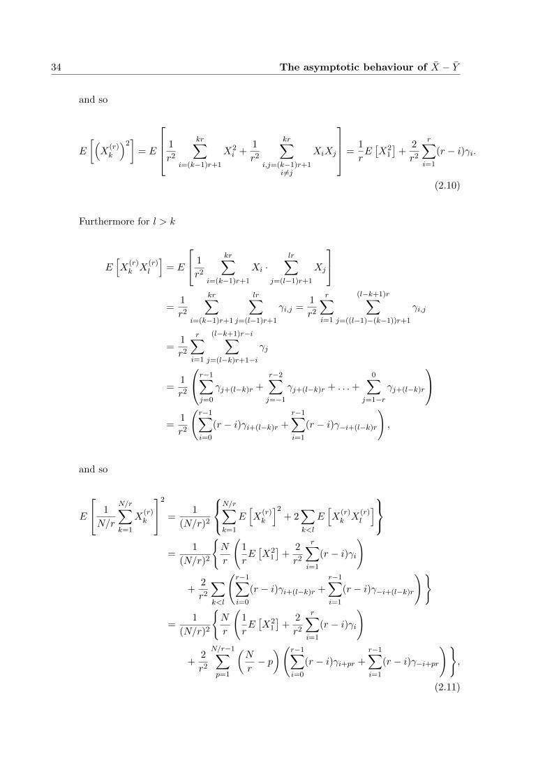
34 The asymptotic behaviour of X − Y
and so
E
[(X
(r)k
)2]
= E
1
r2
kr∑i=(k−1)r+1
X2i +
1
r2
kr∑i,j=(k−1)r+1
i6=j
XiXj
=1
rE[X2
1
]+
2
r2
r∑i=1
(r − i)γi.
(2.10)
Furthermore for l > k
E[X
(r)k X
(r)l
]= E
1
r2
kr∑i=(k−1)r+1
Xi ·lr∑
j=(l−1)r+1
Xj
=
1
r2
kr∑i=(k−1)r+1
lr∑j=(l−1)r+1
γi,j =1
r2
r∑i=1
(l−k+1)r∑j=((l−1)−(k−1))r+1
γi,j
=1
r2
r∑i=1
(l−k+1)r−i∑j=(l−k)r+1−i
γj
=1
r2
r−1∑j=0
γj+(l−k)r +r−2∑j=−1
γj+(l−k)r + . . .+0∑
j=1−rγj+(l−k)r
=
1
r2
(r−1∑i=0
(r − i)γi+(l−k)r +r−1∑i=1
(r − i)γ−i+(l−k)r
),
and so
E
1
N/r
N/r∑k=1
X(r)k
2
=1
(N/r)2
N/r∑k=1
E[X
(r)k
]2+ 2
∑k<l
E[X
(r)k X
(r)l
]=
1
(N/r)2
N
r
(1
rE[X2
1
]+
2
r2
r∑i=1
(r − i)γi
)
+2
r2
∑k<l
(r−1∑i=0
(r − i)γi+(l−k)r +r−1∑i=1
(r − i)γ−i+(l−k)r
)
=1
(N/r)2
N
r
(1
rE[X2
1
]+
2
r2
r∑i=1
(r − i)γi
)
+2
r2
N/r−1∑p=1
(N
r− p)(r−1∑
i=0
(r − i)γi+pr +
r−1∑i=1
(r − i)γ−i+pr
),
(2.11)
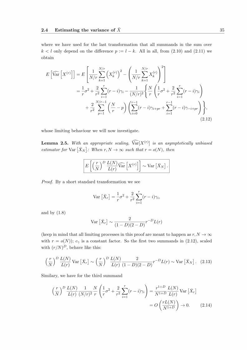
2.4 Estimating the variance of X 35
where we have used for the last transformation that all summands in the sum over
k < l only depend on the difference p := l − k. All in all, from (2.10) and (2.11) we
obtain
E[Var
[X(r)
]]= E
1
N/r
N/r∑k=1
(X
(r)k
)2−
1
N/r
N/r∑k=1
X(r)k
2=
1
rσ2 +
2
r2
r∑i=1
(r − i)γi −1
(N/r)2
N
r
(1
rσ2 +
2
r2
r∑i=1
(r − i)γi
)
+2
r2
N/r−1∑p=1
(N
r− p)(r−1∑
i=0
(r − i)γi+pr +r−1∑i=1
(r − i)γ−i+pr
),
(2.12)
whose limiting behaviour we will now investigate.
Lemma 2.5. With an appropriate scaling, Var[X(r)] is an asymptotically unbiased
estimator for Var[XN
]: When r,N →∞ such that r = o(N), then
E
[( rN
)D L(N)
L(r)Var
[X(r)
]]∼ Var
[XN
].
Proof. By a short standard transformation we see
Var[Xr
]=
1
rσ2 +
2
r2
r∑i=1
(r − i)γi,
and by (1.8)
Var[Xr
]∼ 2
(1−D)(2−D)r−DL(r)
(keep in mind that all limiting processes in this proof are meant to happen as r,N →∞with r = o(N)); cγ is a constant factor. So the first two summands in (2.12), scaled
with (r/N)D, behave like this:
( rN
)D L(N)
L(r)Var
[Xr
]∼( rN
)D L(N)
L(r)
2
(1−D)(2−D)r−DL(r) ∼ Var
[XN
]. (2.13)
Similary, we have for the third summand
( rN
)D L(N)
L(r)
1
(N/r)2
N
r
(1
rσ2 +
2
r2
r∑i=1
(r − i)γi
)=
r1+D
N1+D
L(N)
L(r)Var
[Xr
]= O
(rL(N)
N1+D
)→ 0. (2.14)
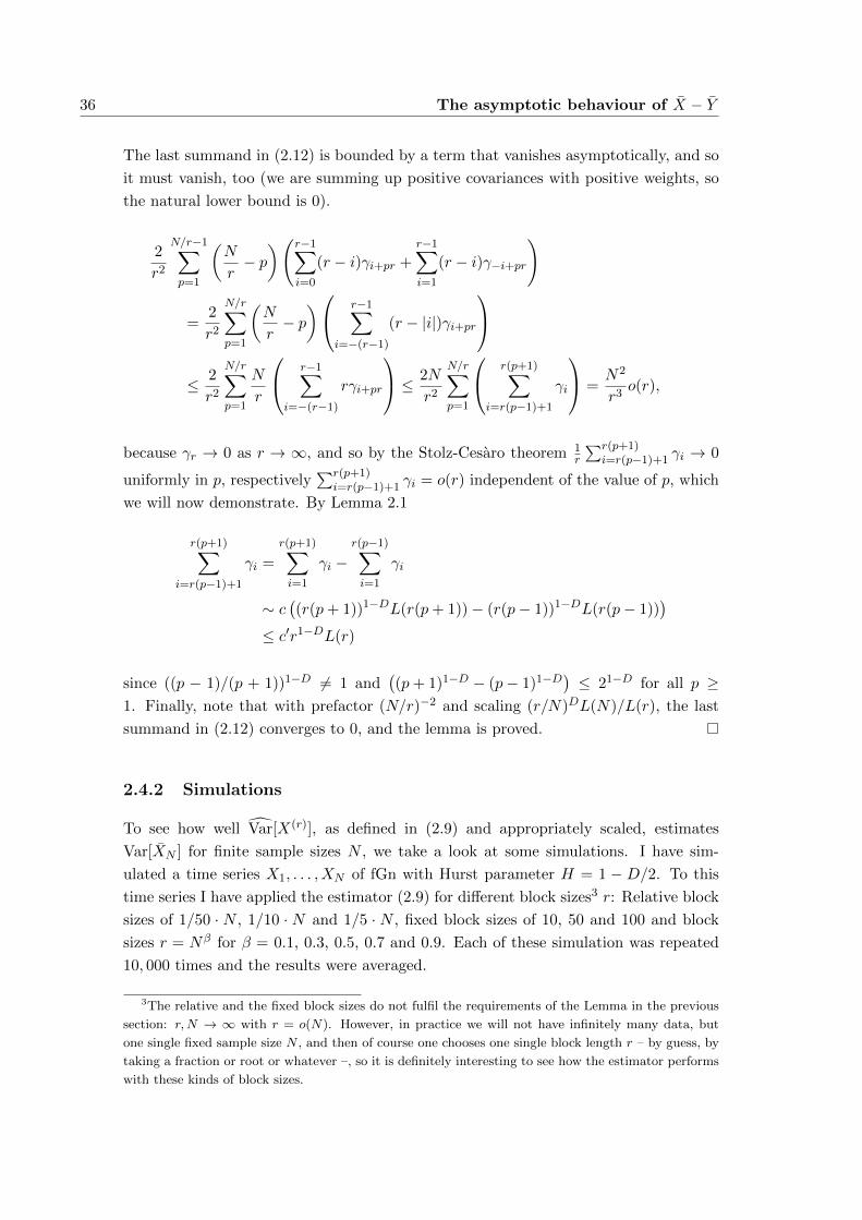
36 The asymptotic behaviour of X − Y
The last summand in (2.12) is bounded by a term that vanishes asymptotically, and so
it must vanish, too (we are summing up positive covariances with positive weights, so
the natural lower bound is 0).
2
r2
N/r−1∑p=1
(N
r− p)(r−1∑
i=0
(r − i)γi+pr +
r−1∑i=1
(r − i)γ−i+pr
)
=2
r2
N/r∑p=1
(N
r− p) r−1∑
i=−(r−1)
(r − |i|)γi+pr
≤ 2
r2
N/r∑p=1
N
r
r−1∑i=−(r−1)
rγi+pr
≤ 2N
r2
N/r∑p=1
r(p+1)∑i=r(p−1)+1
γi
=N2
r3o(r),
because γr → 0 as r → ∞, and so by the Stolz-Cesaro theorem 1r
∑r(p+1)i=r(p−1)+1 γi → 0
uniformly in p, respectively∑r(p+1)
i=r(p−1)+1 γi = o(r) independent of the value of p, which
we will now demonstrate. By Lemma 2.1
r(p+1)∑i=r(p−1)+1
γi =
r(p+1)∑i=1
γi −r(p−1)∑i=1
γi
∼ c((r(p+ 1))1−DL(r(p+ 1))− (r(p− 1))1−DL(r(p− 1))
)≤ c′r1−DL(r)
since ((p − 1)/(p + 1))1−D 6= 1 and((p+ 1)1−D − (p− 1)1−D) ≤ 21−D for all p ≥
1. Finally, note that with prefactor (N/r)−2 and scaling (r/N)DL(N)/L(r), the last
summand in (2.12) converges to 0, and the lemma is proved.
2.4.2 Simulations
To see how well Var[X(r)], as defined in (2.9) and appropriately scaled, estimates
Var[XN ] for finite sample sizes N , we take a look at some simulations. I have sim-
ulated a time series X1, . . . , XN of fGn with Hurst parameter H = 1 − D/2. To this
time series I have applied the estimator (2.9) for different block sizes3 r: Relative block
sizes of 1/50 · N , 1/10 · N and 1/5 · N , fixed block sizes of 10, 50 and 100 and block
sizes r = Nβ for β = 0.1, 0.3, 0.5, 0.7 and 0.9. Each of these simulation was repeated
10, 000 times and the results were averaged.
3The relative and the fixed block sizes do not fulfil the requirements of the Lemma in the previous
section: r,N → ∞ with r = o(N). However, in practice we will not have infinitely many data, but
one single fixed sample size N , and then of course one chooses one single block length r – by guess, by
taking a fraction or root or whatever –, so it is definitely interesting to see how the estimator performs
with these kinds of block sizes.
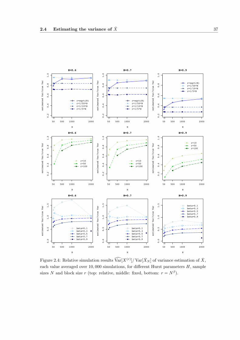
2.4 Estimating the variance of X 37
0.2
0.4
0.6
0.8
1.0
H=0.6
N
estimated Var/true Var
50 500 1000 2000
r=sqrt(N)r=1/50*Nr=1/10*Nr=1/5*N
0.2
0.4
0.6
0.8
1.0
H=0.7
N
estimated Var/true Var
50 500 1000 2000
r=sqrt(N)r=1/50*Nr=1/10*Nr=1/5*N
0.2
0.4
0.6
0.8
1.0
H=0.9
N
estimated Var/true Var
50 500 1000 2000
r=sqrt(N)r=1/50*Nr=1/10*Nr=1/5*N
0.2
0.4
0.6
0.8
1.0
H=0.6
N
estimated Var/true Var
50 500 1000 2000
r=10r=50r=100
0.2
0.4
0.6
0.8
1.0
H=0.7
N
estimated Var/true Var
50 500 1000 2000
r=10r=50r=100
0.2
0.4
0.6
0.8
1.0
H=0.9
N
estimated Var/true Var
50 500 1000 2000
r=10r=50r=100
0.0
0.5
1.0
1.5
H=0.6
N
estimated Var/true Var
50 500 1000 2000
beta=0.1beta=0.3beta=0.5beta=0.7beta=0.9
0.0
0.5
1.0
1.5
H=0.7
N
estimated Var/true Var
50 500 1000 2000
beta=0.1beta=0.3beta=0.5beta=0.7beta=0.9
0.0
0.5
1.0
1.5
H=0.9
N
estimated Var/true Var
50 500 1000 2000
beta=0.1beta=0.3beta=0.5beta=0.7beta=0.9
Figure 2.4: Relative simulation results Var[X(r)]/Var[XN ] of variance estimation of X,
each value averaged over 10, 000 simulations, for different Hurst parameters H, sample
sizes N and block size r (top: relative, middle: fixed, bottom: r = Nβ).
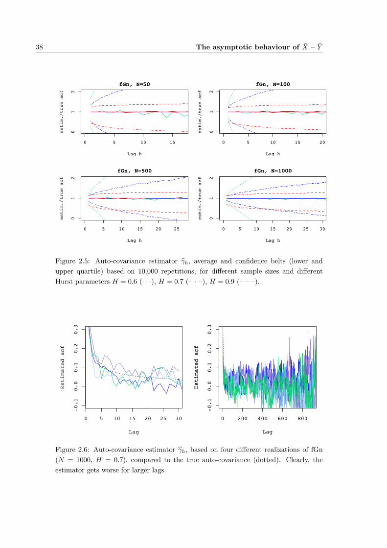
38 The asymptotic behaviour of X − Y
0 5 10 15
fGn, N=50
Lag h
estim./true acf
01
2
0 5 10 15 20
fGn, N=100
Lag h
estim./true acf
01
2
0 5 10 15 20 25
fGn, N=500
Lag h
estim./true acf
01
2
0 5 10 15 20 25 30
fGn, N=1000
Lag h
estim./true acf
01
2
Figure 2.5: Auto-covariance estimator γh, average and confidence belts (lower and
upper quartile) based on 10,000 repetitions, for different sample sizes and different
Hurst parameters H = 0.6 (· · ·), H = 0.7 (– · –), H = 0.9 (– – –).
0 5 10 15 20 25 30
-0.1
0.0
0.1
0.2
0.3
Lag
Estimated acf
0 200 400 600 800
-0.1
0.0
0.1
0.2
0.3
Lag
Estimated acf
Figure 2.6: Auto-covariance estimator γh, based on four different realizations of fGn
(N = 1000, H = 0.7), compared to the true auto-covariance (dotted). Clearly, the
estimator gets worse for larger lags.
2.5 Estimating the auto-covariance 39
The simulation results, i.e. the estimated variance of X relative to the true variance4,
Var[X(r)]/Var[XN ], are shown in Figure 2.4. The exact simulation results are given in
Appendix D.2.
Some values have not been computed because the number of blocks was smaller than
2 or equal or greater than N , which does not make sense. Apparently, relative block
sizes do not perform better with increasing sample size N . As one expects, dividing
the sample in only 5 blocks yields a very poor result. It gets better when the number
of blocks is 50.
If the blocks are of size√N , the estimator becomes better with increasing sample
sizes (from N = 50 to N = 2000 it gains about 20 percentage points).
Fixed block sizes (the second table of each trio) get better with increasing sample
size N as well. In ordinary dimension (a few hundred observations), a block size of
r = 10 is quite respectable.
Polynomial growing block sizes also gain accuracy when N grows. While block sizes
r = N0.1 are unpractical (they tend to overestimate the true variances, in parts with
some ten percent), r = N0.3 seems to be reliable: For all sample sizes it gives a good
approximation to the true variance.
Let us finally look how the estimators handle different levels of long memory. All
types of block sizes yield poorer results when H increases. For H = 0.9, the estimated
variance is alarmingly often less than 50% of the true variance. So estimating the
variance of the mean by block techniques is obviously the more difficult, the stronger
the dependencies are.
2.5 Estimating the auto-covariance
In the following, we will need some higher and mixed moments. They can be calculated
via the diagram formula, see e.g. Major (1981a, Cor. 5.5) or Surgailis (2003).
Lemma 2.6 (Diagram formula). For zero mean Gaussian random variables X1, . . . , Xp,
p ≥ 2, with E[X2j ] = 1 and γi,j := E [XiXj ], i, j = 1, . . . , p it holds
E[Hk1(X1) · · ·Hkp(Xp)
]=
k1!···kp!
2qq!
∑′γi1,j1 · · · γiq ,jq k1 + . . .+ kp = 2q and
0 ≤ k1, . . . , kq ≤ q
0 otherwise
,
where∑′
denotes a sum over all indices i1, j1, · · · iq, jq with
• i1, j1, . . . , iq, jq ∈ 1, 2, . . . , p
• i1 6= j1, . . . , iq 6= jq
4Since the auto-covariances γk of fGn are known, see (1.4), Var[XN ] = nγ0 + 2∑N−1k=1 (N − k)γk can
be calculated.
40 The asymptotic behaviour of X − Y
• k1 indices are 1, k2 indices are 2, . . . , kp indices are p.
Example. We will consider some examples in order to illustrate the use of the diagram
formula and to prepare the upcoming calculations.
1. Let i, j, k, l be pairwise different indices.
E[XiXjXkXl] =1
8(8γi,jγk,l + 8γi,kγj,l + 8γi,lγj,k) , (2.15)
respectively in the special case when i 6= j, k = i + h 6= j and l = j + h 6= i for
h > 0
E[XiXjXi+hXj+h] =1
2
(γ2i,j + γ2
h + γi,j+hγj,i+h).
E[X2iX
2j ] = E[(X2
i − 1)(X2j − 1)] + E
[X2i
]+ E
[X2j
]− 1
= E [H2(Xi)H2(Xj)] + 1 =1
24γ2
i,j + 1 (2.16)
E[XiXjX2k ] = E [H1(Xi)H1(Xj)H2(Xk)] + E [XiXj ]
=1
228γi,kγj,k + γi,j = 2γi,kγj,k + γi,j (2.17)
2. Consider Hermite polynomials Hk, k ∈ N.
E[Hki(Xi)Hkj (Xj)
]=
ki!kj !2qq!
∑′γi1,j1 · · · γiq ,jq ki + kj = 2q and
0 ≤ ki, kj ≤ q
0 otherwise.
If ki 6= kj , E[Hki(Xi)Hkj (Xj)] = 0, since if ki + kj are even, i.e. ki + kj = 2q for
a number q ∈ N, then either ki, kj are both even or both are odd. Let w.l.o.g.
ki > kj , then ki = kj + 2k, k ∈ N. It follows ki + kj = 2kj + 2k = 2q, thus
kj + k = q, and that means ki = kj + 2k = q + k > q.
If ki = kj =: k, we have q = k and
E[Hki(Xi)Hkj (Xj)
]= E [Hk(Xi)Hk(Xj)] =
k!
2k
∑′
γi1,j1 · · · γiq ,jq ,
where∑′
denotes a sum over all indices i1, j1, · · · iq, jq such that k1 indices are 1,
k2 indices are 2, . . . , kp indices are p, in other words k indices are i and k indices
are j. Since the indices must be pairwise different, i1 6= j1, . . . , iq 6= jq, the sum is∑′γi,j · · · γi,j and each summand consists of k factors. How many such summands
are possible? Each factor is γi,j or γj,i, so each factor has two possibilities, thus
there are 2k possible summands in∑′
. So we obtain
E[Hki(Xi)Hkj (Xj)
]= k!γki,j .
We have just established (1.6).
2.5 Estimating the auto-covariance 41
3. We will now verify (1.7) as well, applying the just proved formula (1.6):
E
[N∑i=1
Hk(Xi)
]2
= E
[N∑i=1
Hk(Xi)Hk(Xi)
]+ E
N∑i6=j
Hk(Xi)Hk(Xj)
= Nk! +
N∑i6=j
k!γki,j ,
which yields (1.7) with γk = γi,i+k = Cov[Xi, Xi+k] = k−DL(k).
2.5.1 Asymptotic behaviour of the auto-covariance estimator
We will use the diagram formula to prove
Theorem 2.7. The standard estimator for the auto-covariances γh = Cov [Xi, Xi+h]
γh =1
N − h
N−h∑i=1
XiXi+h (2.18)
is asymptotically consistent for all fixed h ∈ N as N →∞:
E [γh] = γh, Var [γh]→ 0
This is comforting to know.
Proof. Unbiasedness is immediate. The asymptotic zero variance requires some more
effort. First consider the case h = 0. Then
Var[γ0] =1
N2Var
[N∑i=1
X2i
]=
1
N2Var
[N∑i=1
H2(Xi)
]
and this converges to 0 due to (1.8). If h > 0, we set M := N − h. We will show that
Var [γh] ≤ O(M−1) +O(M−DL(M)), (2.19)
so that Var [γh] → 0 not uniformly in h as N → ∞, but in some sense uniformly over
certain sets of values for N,h. We will make use of this in a later proof. Now write
Var [γh] =1
M2
E [ M∑i=1
XiXi+h
]2
− (Mγh)2
=
1
M2
M∑i=1
E[X2iX
2i+h
]+ 2
M∑i<j
E [XiXi+hXjXj+h]
− γ2h. (2.20)
42 The asymptotic behaviour of X − Y
The first sum is bounded by O(M). We will now show that the second sum, scaled with
M−2, converges to γ2h. In order to apply the diagram formula, we have to distinguish
two cases: i+ h = j and i+ h 6= j.
2
M∑i<j
E [XiXi+hXjXj+h] = 2
M−h∑i=1
E[XiX
2jXj+h
]+ 2
M∑i<j,j 6=i+h
E [XiXi+hXjXj+h]
= O(M) + 2M−1∑
k=1,k 6=h(M − k)(γ2
k + γ2h + γk+hγ|k−h|),
where in the last step we have used that the covariances in the sum over i < j depend
only on the lag k = j− i, and below the diagonal i = j there are (M−k) indices (i, j)
with lag k. Now γk = E[XiXi+k] ≤ (E[X2i ]E[X2
i+k])1/2 = 1, and so we can roughly
estimate
M−1∑k=1,k 6=h
(M − k)γ2k ≤
M∑k=1
(M − k)γk ∼ c ·M2−DL(M)
where c is a constant, due to (B.6) which follows from Karamata’s Theorem, similar to
(2.6). The same upper bound holds for∑M−1
k=1,k 6=h(M − k)γk+hγ|k−h|, and so both sums
are o(M2). Finally note that
2M−1∑
k=1,k 6=h(M − k) ≤ 2
M∑k=1
(M − k) = 2
(M2 − M(M + 1)
2
),
thus
Var [γh] ≤ O(M−1) +O(M−DL(M)) +
∣∣∣∣2(1− M(M + 1)
2M2
)− 1
∣∣∣∣ ,which proves (2.19).
2.5.2 Simulations
By Theorem 2.7, the standard auto-covariance estimator
γh =1
N − h
N−h∑i=1
XiXi+h,
as defined in (2.18), is asymptotically unbiased. We will now investigate its performance
in finite sample situations by a simulation study. To this end, we have simulated
samples of fGn of length N (with N = 50, 100, 500, 1000). fGn has the exact auto-
covariances (1.4). For each sample we have calculated the estimated auto-covariances
γh, h = 1, . . . , N − 1. Each simulation was repeated 10,000 times; so based on these
10,000 repetitions, for each lag h, we have calculated an average value of γh and the
lower and upper quartile. The results are presented in Figure 2.5, where the simulation
results are shown, relative to the true auto-covariance (1.4).
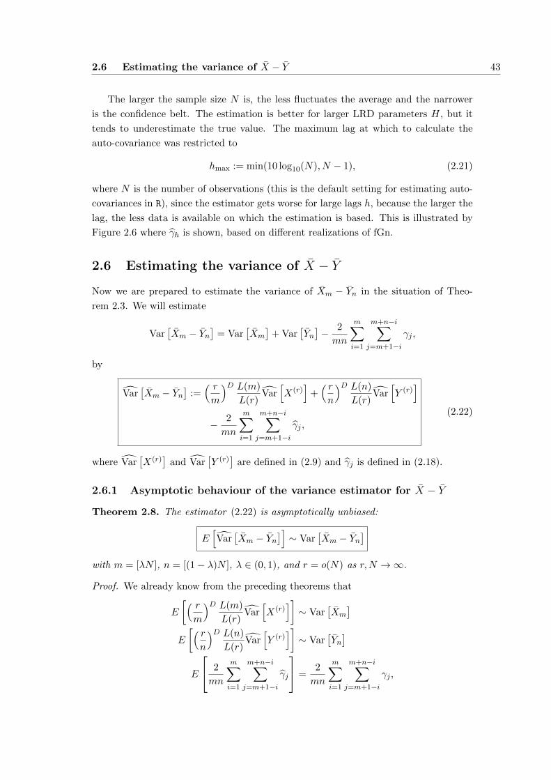
2.6 Estimating the variance of X − Y 43
The larger the sample size N is, the less fluctuates the average and the narrower
is the confidence belt. The estimation is better for larger LRD parameters H, but it
tends to underestimate the true value. The maximum lag at which to calculate the
auto-covariance was restricted to
hmax := min(10 log10(N), N − 1), (2.21)
where N is the number of observations (this is the default setting for estimating auto-
covariances in R), since the estimator gets worse for large lags h, because the larger the
lag, the less data is available on which the estimation is based. This is illustrated by
Figure 2.6 where γh is shown, based on different realizations of fGn.
2.6 Estimating the variance of X − Y
Now we are prepared to estimate the variance of Xm − Yn in the situation of Theo-
rem 2.3. We will estimate
Var[Xm − Yn
]= Var
[Xm
]+ Var
[Yn]− 2
mn
m∑i=1
m+n−i∑j=m+1−i
γj ,
by
Var[Xm − Yn
]:=( rm
)D L(m)
L(r)Var
[X(r)
]+( rn
)D L(n)
L(r)Var
[Y (r)
]− 2
mn
m∑i=1
m+n−i∑j=m+1−i
γj ,
(2.22)
where Var[X(r)
]and Var
[Y (r)
]are defined in (2.9) and γj is defined in (2.18).
2.6.1 Asymptotic behaviour of the variance estimator for X − Y
Theorem 2.8. The estimator (2.22) is asymptotically unbiased:
E[Var
[Xm − Yn
]]∼ Var
[Xm − Yn
]with m = [λN ], n = [(1− λ)N ], λ ∈ (0, 1), and r = o(N) as r,N →∞.
Proof. We already know from the preceding theorems that
E
[( rm
)D L(m)
L(r)Var
[X(r)
]]∼ Var
[Xm
]E
[( rn
)D L(n)
L(r)Var
[Y (r)
]]∼ Var
[Yn]
E
2
mn
m∑i=1
m+n−i∑j=m+1−i
γj
=2
mn
m∑i=1
m+n−i∑j=m+1−i
γj ,
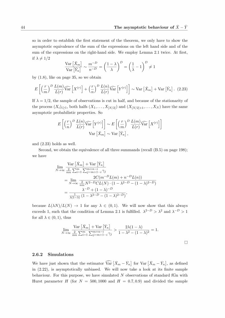
44 The asymptotic behaviour of X − Y
so in order to establish the first statement of the theorem, we only have to show the
asymptotic equivalence of the sum of the expressions on the left hand side and of the
sum of the expressions on the right-hand side. We employ Lemma 2.1 twice. At first,
if λ 6= 1/2
Var[Xm
]Var
[Yn] ∼ m−D
n−D=
(1− λλ
)D=
(1
λ− 1
)D6= 1
by (1.8), like on page 35, so we obtain
E
[( rm
)D L(m)
L(r)Var
[X(r)
]+( rn
)D L(n)
L(r)Var
[Y (r)
]]∼ Var
[Xm
]+ Var
[Yn]. (2.23)
If λ = 1/2, the sample of observations is cut in half, and because of the stationarity of
the process (Xi)i≥1, both halfs (X1, . . . , X[N/2]) and (X[N/2]+1, . . . , XN ) have the same
asymptotic probabilistic properties. So
E
[( rn
)D L(n)
L(r)Var
[Y (r)
]]∼ E
[( rm
)D L(m)
L(r)Var
[X(r)
]]Var
[Xm
]∼ Var
[Yn],
and (2.23) holds as well.
Second, we obtain the equivalence of all three summands (recall (B.5) on page 198);
we have
limN→∞
Var[Xm
]+ Var
[Yn]
2mn
∑mi=1
∑m+n−ij=m+1−i γj
= limN→∞
2C(m−DL(m) + n−DL(n))2nmN
2−DCL(N) · (1− λ2−D − (1− λ)2−D)
=λ−D + (1− λ)−D
1λ(1−λ) (1− λ2−D − (1− λ)2−D)
,
because L(λN)/L(N) → 1 for any λ ∈ (0, 1). We will now show that this always
exceeds 1, such that the condition of Lemma 2.1 is fulfilled. λ2−D > λ2 and λ−D > 1
for all λ ∈ (0, 1), thus
limN→∞
Var[Xm
]+ Var
[Yn]
2mn
∑mi=1
∑m+n−ij=m+1−i γj
>2λ(1− λ)
1− λ2 − (1− λ)2= 1.
2.6.2 Simulations
We have just shown that the estimator Var[Xm − Yn
]for Var
[Xm − Yn
], as defined
in (2.22), is asymptotically unbiased. We will now take a look at its finite sample
behaviour. For this purpose, we have simulated N observations of standard fGn with
Hurst parameter H (for N = 500, 1000 and H = 0.7, 0.9) and divided the sample
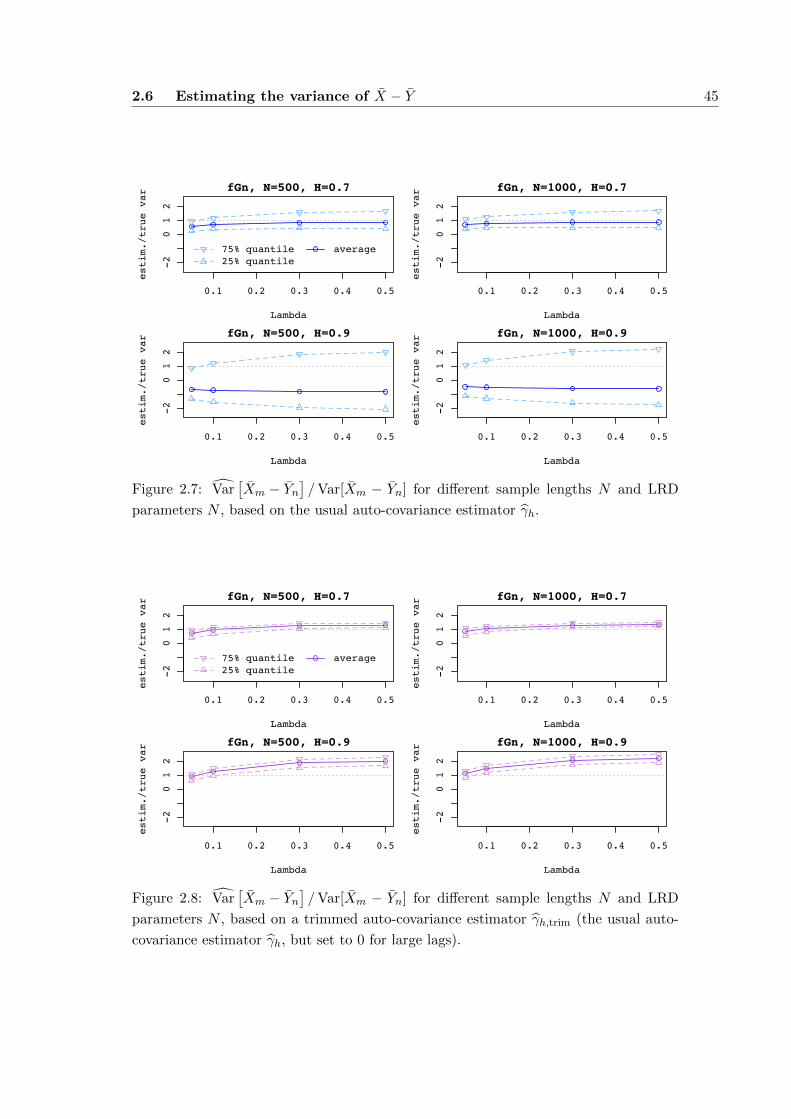
2.6 Estimating the variance of X − Y 45
0.1 0.2 0.3 0.4 0.5
-2
01
2
fGn, N=500, H=0.7
Lambda
estim./true var
75% quantile25% quantile
average
0.1 0.2 0.3 0.4 0.5
-2
01
2
fGn, N=1000, H=0.7
Lambda
estim./true var
0.1 0.2 0.3 0.4 0.5
-2
01
2
fGn, N=500, H=0.9
Lambda
estim./true var
0.1 0.2 0.3 0.4 0.5-2
01
2
fGn, N=1000, H=0.9
Lambda
estim./true var
Figure 2.7: Var[Xm − Yn
]/Var[Xm − Yn] for different sample lengths N and LRD
parameters N , based on the usual auto-covariance estimator γh.
0.1 0.2 0.3 0.4 0.5
-2
01
2
fGn, N=500, H=0.7
Lambda
estim./true var
75% quantile25% quantile
average
0.1 0.2 0.3 0.4 0.5
-2
01
2
fGn, N=1000, H=0.7
Lambda
estim./true var
0.1 0.2 0.3 0.4 0.5
-2
01
2
fGn, N=500, H=0.9
Lambda
estim./true var
0.1 0.2 0.3 0.4 0.5
-2
01
2
fGn, N=1000, H=0.9
Lambda
estim./true var
Figure 2.8: Var[Xm − Yn
]/Var[Xm − Yn] for different sample lengths N and LRD
parameters N , based on a trimmed auto-covariance estimator γh,trim (the usual auto-
covariance estimator γh, but set to 0 for large lags).
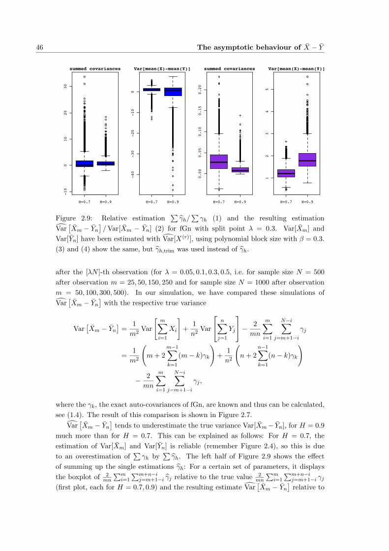
46 The asymptotic behaviour of X − Y
-10
010
2030
summed covariances
H=0.7 H=0.9
-40
-30
-20
-10
0
Var[mean(X)-mean(Y)]
H=0.7 H=0.90.00
0.05
0.10
0.15
0.20
summed covariances
H=0.7 H=0.9
12
34
5
Var[mean(X)-mean(Y)]
H=0.7 H=0.9
Figure 2.9: Relative estimation∑γh/
∑γh (1) and the resulting estimation
Var[Xm − Yn
]/Var[Xm − Yn] (2) for fGn with split point λ = 0.3. Var[Xm] and
Var[Yn] have been estimated with Var[X(r)], using polynomial block size with β = 0.3.
(3) and (4) show the same, but γh,trim was used instead of γh.
after the [λN ]-th observation (for λ = 0.05, 0.1, 0.3, 0.5, i.e. for sample size N = 500
after observation m = 25, 50, 150, 250 and for sample size N = 1000 after observation
m = 50, 100, 300, 500). In our simulation, we have compared these simulations of
Var[Xm − Yn
]with the respective true variance
Var[Xm − Yn
]=
1
m2Var
[m∑i=1
Xi
]+
1
n2Var
n∑j=1
Yj
− 2
mn
m∑i=1
N−i∑j=m+1−i
γj
=1
m2
(m+ 2
m−1∑k=1
(m− k)γk
)+
1
n2
(n+ 2
n−1∑k=1
(n− k)γk
)
− 2
mn
m∑i=1
N−i∑j=m+1−i
γj ,
where the γk, the exact auto-covariances of fGn, are known and thus can be calculated,
see (1.4). The result of this comparison is shown in Figure 2.7.
Var[Xm − Yn
]tends to underestimate the true variance Var[Xm− Yn], for H = 0.9
much more than for H = 0.7. This can be explained as follows: For H = 0.7, the
estimation of Var[Xm] and Var[Yn] is reliable (remember Figure 2.4), so this is due
to an overestimation of∑γh by
∑γh. The left half of Figure 2.9 shows the effect
of summing up the single estimations γh: For a certain set of parameters, it displays
the boxplot of 2mn
∑mi=1
∑m+n−ij=m+1−i γj relative to the true value 2
mn
∑mi=1
∑m+n−ij=m+1−i γj
(first plot, each for H = 0.7, 0.9) and the resulting estimate Var[Xm − Yn
]relative to
2.6 Estimating the variance of X − Y 47
the true value Var[Xm − Yn
](second plot, each for H = 0.7, 0.9). Indeed, we observe
a huge variance for∑γh with more upper outliers than lower ones. When H = 0.9,
then Var[Xm] and Var[Yn] are underestimated (as shown in Figure 2.4), and moreover,
as Figure 2.9 demonstrates,∑γh heavily overestimates
∑γh, and we have only upper
outliers. In consequence, recall the definition (2.22), Var[Xm − Yn
]gets much too
small.
An improvement can simply be obtained by adjusting the auto-covariance estimator
γh which is involved in Var[Xm − Yn
]and which is bad for large lags, as we have
just illustrated in Figure 2.6; a natural idea is to trimm it. If we estimate the auto-
covariances γh by
γh,trim =
γh if h ≤ hmax
0 else,
with hmax as in (2.21), and use this as auto-covariance estimator in Var[Xm − Yn
], the
estimation gets better: As shown in Figure 2.8, the confidence belts become narrower,
and especially for H = 0.9, the average gets closer to the true variance (even though
it now exceeds it). The right half of Figure 2.9 confirms that trimming improves the
estimation of∑γh by
∑γh: Now, we do not obtain this broad range of outliers, and
as a consequence Var[Xm − Yn
]yields better results.

48 The asymptotic behaviour of X − Y

Chapter 3
A “Wilcoxon-type” change-point
test
In this chapter we develop a non-parametric change-point test for changes in the mean of
LRD processes that have a representation as an instantaneous functional of a stationary
Gaussian process. We aim at a test which is based on the Wilcoxon two-sample test
statistic, roughly speaking a “Wilcoxon-type” test.
Wilcoxon’s rank statistic can be represented as a U -statistic, so a natural approach
is to rely on the work of Dehling and Taqqu (1989) who derived a limit theorem for
one-sample U -statistics of LRD data. Unfortunately, the technical requirements forbid
to extend the method as a whole to the Wilcoxon two-sample test statistic; the crucial
point is that the kernel of the U -statistic has to have bounded variation, but h(x, y) =
Ix≤y, which is the kernel that leads to Wilcoxon’s two-sample test statistic, does not
have this property.
In this chapter, we will thus make a different approach: We represent the Wilcoxon
two-sample test statistic as a functional of the one-dimensional empirical process and
apply to this the limit theorem of Dehling and Taqqu (1989). This part of this work is
based on the article of Dehling, Rooch and Taqqu (2012).
In what follows, we define our test and derive its asymptotic distribution under
the null hypothesis that no change occured. In a subsequent simulation study, we also
compare its power with the power of a test which is based on differences of means in a
simulation study. We will see that for Gaussian data, the non-parametric change-point
test has only a slightly smaller power, while for heavy-tailed data it outperforms the
“difference-of-means” test. Motivated by these observations, we will compare the power
of both tests analytically; this is carried out in the next chapter.
50 A “Wilcoxon-type” change-point test
3.1 Setting the scene
We consider observations (Xi)i≥1 of the type
Xi = µi + εi,
where (µi)i≥1 are unknown means and (εi)i≥1 is an instantaneous functional of a
stationary Gaussian process with non-summable covariances, i.e.
εi = G(ξi), i ≥ 1,
where (ξi)i≥1 is a mean-zero Gaussian process with E(ξ2i ) = 1 and long-range depen-
dence, that is, with auto-covariance function (1.1). G is a measurable transformation
which fulfills some technical requirements.
Definition 3.1 (Centralized/normalized Lp(R)-functions). Let ξ ∼ N (0, 1) be a stan-
dard normal random variable. We define
G1 = G1(R,N ) := G : R→ R measurable | E[G(ξ)] = 0 ⊂ L1(R,N ),
the class of (with respect to the standard normal measure) centralized and integrable
functions, and
G2 = G2(R,N ) := G : R→ R measurable | E[G(ξ)] = 0, E[G2(ξ)] = 1 ⊂ L2(R,N ),
the class of (with respect to the standard normal measure) normalized and square-
integrable functions.
Any transformation G : R → R which is measurable with mean zero and finite
variance under standard normal measure can be normalized by dividing the standard
deviation, so it can be considered as a function in G2. In the following, G is either in
G1 or in G2. So after all, the observations (Xi)i≥1 are always assumed to be an LRD
stationary process with mean zero.
Based on the observations X1, . . . , Xn, we wish to test the hypothesis
H : µ1 = . . . = µn (3.1)
that there is no change in the means of the data against the alternative
A : µ1 = . . . = µk 6= µk+1 = . . . = µn for some k ∈ 1, . . . , n− 1 (3.2)
that there is an index after which the level shifts. We shall refer to this test problem
as (H,A).
A usual approach to change-point tests is to start with a two-sample problem where
the change-point is known; in this case, for a given k ∈ 1, . . . , n− 1, the alternative
is
Ak : µ1 = . . . = µk 6= µk+1 = . . . = µn.

3.2 Limit distribution under null hypothesis 51
For such a test problem (H,Ak), a commonly used non-parametric test is the Wilcoxon
two-sample rank test. It rejects for large and small values of the test statistic
Wk,n =k∑i=1
n∑j=k+1
IXi≤Xj
which counts the number of times the second part of the sample exceeds the first
part of the sample. This is the Mann-Whitney representation of Wilcoxon’s rank test
statistic as a U -statistic (Lehmann, 1975). From this two-sample problem (H,Ak)
with a known change-point, one passes over to the change-point problem (H,A),
where one does not know k, by considering a functional of the vector of test statis-
tics W1,n, . . . ,Wn−1,n. A common procedure is to reject the null hypothesis for large
values of Wn = maxk=1,...,n−1 |Wk,n|. This is what we will do (but of course, other
functions of W1,n, . . . ,Wn−1,n are also possible).
In order to set the critical values of the test, we need to know the asymptotic
distribution of Wn under the null hypothesis of no change (the exact distribution is
hard to obtain, so we have to settle for an asymptotic test), so we want to obtain the
asymptotic distribution for a large sample size and consider the process
W[nλ],n =
[nλ]∑i=1
n∑j=[nλ]+1
IXi≤Xj, 0 ≤ λ ≤ 1,
parametrized by λ. After centering and scaling, where F denotes the c.d.f. of the
Xi = G(ξi) and dn is defined in (1.12), we obtain the process
Wn(λ) =1
ndn
[nλ]∑i=1
n∑j=[nλ]+1
(IXi≤Xj −
∫RF (x)dF (x)
), 0 ≤ λ ≤ 1. (3.3)
Technical remark. The centering constant∫R F (x)dF (x) equals E[IX1≤X′1], where X ′1 is an inde-
pendent copy of X1. It is the proper normalization as the dependence between Xi and Xj vanishes
asymptotically when |j − i| → ∞. Of course, this is only an heuristic argument, but in the course
of the proof we will see that it is just the right centering constant. If the distribution function F is
continuous,∫R F (x)dF (x) = 1
2.
Under the null hypothesis of no change in the mean, the distribution of Wn(λ) does
not depend on the common mean µ := µ1 = . . . = µn, so we may assume without loss
of generality that µ = 0 and hence that Xi = G(ξi).
3.2 The limit distribution under the null hypothesis
Our aim is to analyse the asymptotic distribution of the process (Wn(λ))0≤λ≤1. Since
it has the representation of a U -statistic, a natural idea to handle it is to extend the
52 A “Wilcoxon-type” change-point test
method of Dehling and Taqqu (1989) who treat one-sample U -statistics of LRD data,
but as mentioned in the introduction of the chapter, this approach fails due to the
technical requirements: The kernel h(x, y) = Ix<y does not have bounded variation
(we prove this in few words on page 210; an overview about the concept of bounded
variation in higher dimensions, which may be needed for this, is given in Appendix B.3).
Nevertheless, to analyse the asymptotic distribution of the process (Wn(λ))0≤λ≤1, we
can apply the empirical process invariance principle of Dehling and Taqqu (1989) to
the sequence (G(ξi))i≥1, and this approach succeeds.
We consider the Hermite expansion
IG(ξi)≤x − F (x) =∞∑q=1
Jq(x)
q!Hq(ξi),
where Hq is the q-th order Hermite polynomial and where Jq(x) = E[Hq(ξi)IG(ξi)≤x]
is the belonging Hermite coefficient (depending on x).
Definition 3.2 (Hermite rank of class of functions). We define the Hermite rank of
the class of functions IG(ξi)≤x − F (x), x ∈ R by
m := minq ≥ 1 : Jq(x) 6= 0 for some x ∈ R. (3.4)
Theorem 3.1. Suppose that (ξi)i≥1 is a stationary Gaussian process with mean zero,
variance 1 and auto-covariance function (1.1) with 0 < D < 1m . For G ∈ G1, we define
Xk = G(ξk).
Assume that Xk has a continuous distribution function F . Let m denote the Hermite
rank of the class of functions IG(ξi)≤x − F (x), x ∈ R, as defined in (3.4), and let
dn > 0 satisfy (1.12). Then
1
ndn
[nλ]∑i=1
n∑j=[nλ]+1
(IXi≤Xj −
∫RF (x)dF (x)
), 0 ≤ λ ≤ 1, (3.5)
converges in distribution towards the process
1
m!(Zm(λ)− λZm(1))
∫RJm(x)dF (x), 0 ≤ λ ≤ 1.
Details to the process (Zm(λ))λ≥0 are given in Section 1.4.2 and in the paper of
Dehling and Taqqu (1989). The process is a so called Hermite process, and it is self-
similar with parameter1
H = 1− mD
2∈(
1
2, 1
).
Zm(λ) is not Gaussian when m ≥ 2. When m = 1, Z1(λ) is the standard Gaussian
fBm BH(λ).
1Do not confuse the index H, which is called Hurst parameter, with the other H’s used in this work
to denote for example hypothesis and Hermite polynomial.

3.2 Limit distribution under null hypothesis 53
Proof. We introduce the empirical distribution functions of the first k and the last
(n− k) observations, respectively:
Fk(x) =1
k
k∑i=1
IXi≤x
Fk+1,n(x) =1
n− k
n∑i=k+1
IXi≤x
Thus we have [nλ]F[nλ](x) =∑[nλ]
i=1 IXi≤x and (n−[nλ])F[nλ]+1,n(x) =∑n
i=[nλ]+1 IXi≤x,
and we obtain the following representation:
[nλ]∑i=1
n∑j=[nλ]+1
(IXi≤Xj −
∫RF (x)dF (x)
)(3.6)
= [nλ]n∑
j=[nλ]+1
(F[nλ](Xj)−
∫RF (x)dF (x)
)
= [nλ](n− [nλ])
(∫RF[nλ](x)dF[nλ]+1,n(x)−
∫RF (x)dF (x)
)= [nλ](n− [nλ])
∫R
(F[nλ](x)− F (x))dF[nλ]+1,n(x)
+ [nλ](n− [nλ])
∫RF (x)d(F[nλ]+1,n − F )(x)
= [nλ](n− [nλ])
∫R
(F[nλ](x)− F (x))dF[nλ]+1,n(x)
− [nλ](n− [nλ])
∫R
(F[nλ]+1,n(x)− F (x))dF (x).
In the final step, we have used integration by parts, namely∫RGdF = 1−
∫R F dG, if F
and G are two distribution functions. We now apply the empirical process non-central
limit theorem of Dehling and Taqqu (1989) which states that
(d−1n [nλ](F[nλ](x)− F (x))
)x∈[−∞,∞], λ∈[0,1]
D−→ (J(x)Z(λ))x∈[−∞,∞], λ∈[0,1], (3.7)
where
J(x) = Jm(x) and Z(λ) = Zm(λ)/m!.
By the Dudley-Wichura version of Skorohod’s representation theorem (Shorack and
Wellner, 1986, Th. 2.3.4) we may assume without loss of generality that convergence
holds almost surely with respect to the supremum norm on the function space D([0, 1]×[−∞,∞]), i.e.
supλ,x
∣∣d−1n [nλ](Fnλ(x)− F (x))− J(x)Z(λ)
∣∣ −→ 0 a.s.. (3.8)

54 A “Wilcoxon-type” change-point test
Technical remark. The theorem states: If we have weak convergence, we can find an equivalent
process which converges almost surely. In detail, let (M,d) denote a metric space and let MBd be the
σ-field generated by the collection of all open balls B = y | d(x, y) < r ⊂ M for some x ∈ M and
some r > 0. Now if we have weak convergence of a random process Xn →w X0 on (M,MBd , d), then we
can find equivalent variables Xn =D X′n (which may live on another probability space) which converge
almost surely, as long as the limit variable is concentrated on a separable subset of M : d(X ′n, X′0)→a.s. 0
as n → ∞, as long as P0(Ms) = 1 for a MBd -measurable subset Ms ⊂ M that is d-seperable, i.e. that
has a countable subset d-dense in M .
First, notice that the equivalent process may have another common distribution. But we are only
interested in weak convergence of the process, so we do not need to care about it.
Second, the convergence in (3.7) happens in D((−∞,∞) × [0, 1]) which is not separable, but the
limit J(x)Z(λ) can be regarded as an element of C((−∞,∞)× [0, 1]) which is. To see this, note that
Z(λ) can be assumed to be a version with continuous sample paths, and that J(x) does not have jumps
as long as Xk has a continuous c.d.f. F (t) = P (G(Y ) ≤ t):
J(t) =
∫IG(y)≤tHq(y) dΦ(y) =
∫y|G(y)≤t
Hq(y) dPY (y) =
∫ω|G(Y (ω))≤t
Hq(Y (ω)) dP (ω),
so the domain of integration (more precisely: its measure under P ) changes continuously with t, and
Hq is smooth.
(3.8) is a result on the e.d.f. of the first [λn] observations. We can deduce a similar
result on the e.d.f. of the remaining n− [λn] observations X[nλ]+1, . . . , Xn:
supλ,x
∣∣d−1n (n− [nλ])(F[nλ]+1,n(x)− F (x))− J(x)(Z(1)− Z(λ))
∣∣ −→ 0 a.s.. (3.9)
To see this, consider the empirical processes of all n and of the initial [λn] observations,
n (Fn(x)− F (x)) =
n∑i=1
(IXi≤x − F (x)
)[nλ]
(F[nλ](x)− F (x)
)=
[nλ]∑i=1
(IXi≤x − F (x)
).
By definition, we have
(n− [nλ])(F[nλ]+1,n(x)− F (x)
)=
n∑i=[nλ]+1
(IXi≤x − F (x)
),
and this equals (take the difference on both sides between the two lines above)
n (Fn(x)− F (x))− [nλ](F[nλ](x)− F (x)
),
so we can deduce (3.9) in this way:
supλ,x
d−1n (n− [λn])
∣∣(F[nλ+1,n](x)− F (x))− J(x) (Z(1)− Z(λ))
∣∣≤ sup
λ,xd−1n
(n |(Fn(x)− F (x))− J(x)Z(1)|+ [nλ]
∣∣(F[nλ](x)− F (x))− J(x)Z(λ)
∣∣) ,and both terms vanish by (3.8).

3.2 Limit distribution under null hypothesis 55
Thus we get, for the first term in the right-hand side of (3.6),
1
ndn[nλ](n− [nλ])
∫R
(F[nλ](x)− F (x))dF[nλ]+1,n(x)− (1− λ)
∫RJ(x)Z(λ)dF (x)
(3.10)
=n− [nλ]
n
∫Rd−1n [nλ](F[nλ](x)− F (x))dF[nλ]+1,n(x)− n− [nλ]
n
∫RJ(x)Z(λ)dF (x)
+
n− [nλ]
n− (1− λ)
∫RJ(x)Z(λ)dF (x)
=n− [nλ]
n
∫R
d−1n [nλ](F[nλ](x)− F (x))− J(x)Z(λ)
dF[nλ]+1,n(x)
+n− [nλ]
n
∫RJ(x)Z(λ)d(F[nλ]+1,n − F )(x)
+
n− [nλ]
n− (1− λ)
∫RJ(x)Z(λ)dF (x).
The first term on the right-hand side converges to 0 almost surely by (3.8). The third
term converges to zero as
sup0≤λ≤1
∣∣∣∣n− [nλ]
n− (1− λ)
∣∣∣∣→ 0,
because with nλ− 1 ≤ [nλ] ≤ nλ+ 1, we obtain
∣∣∣∣n− [nλ]
n− (1− λ)
∣∣∣∣ =
∣∣∣∣λ− [nλ]
n
∣∣∣∣ ≤ ∣∣∣∣λ− nλ+ 1
n
∣∣∣∣ =1
n.
Regarding the second term, note that∫R J(x)dF (x) = E(J(Xi)) and hence
n− [nλ]
n
∫RJ(x)Z(λ)d(F[nλ]+1,n − F )(x)
= Z(λ)1
n
n∑i=[nλ]+1
(J(Xi)− EJ(Xi))
= Z(λ)
1
n
n∑i=1
(J(Xi)− E(J(Xi)))−1
n
[nλ]∑i=1
(J(Xi)− E(J(Xi)))
.
56 A “Wilcoxon-type” change-point test
By the ergodic theorem2 , 1n
∑ni=1(J(Xi) − E(J(Xi))) → 0, almost surely. Hence∑n
i=1(J(Xi)− E(J(Xi))) = o(n) and thus
max1≤k≤n
∣∣∣∣∣k∑i=1
(J(Xi)− E(J(Xi)))
∣∣∣∣∣ = o(n), as n→∞, a.s.,
otherwise 1n
∑ni=1(J(Xi)−E(J(Xi))) would possess a subsequence which does not con-
vergece to 0. Hence (3.10) converges to zero almost surely, uniformly in λ ∈ [0, 1].
Regarding the second term on the right-hand side of (3.6) we obtain
1
ndn[nλ](n− [nλ])
∫R
(F[nλ]+1,n − F (x))dF (x)− λ∫RJ(x)(Z(1)− Z(λ))dF (x) (3.11)
=[nλ]
n
∫R
d−1n (n− [nλ])(F[λn]+1,n(x)− F (x))− J(x)(Z(1)− Z(λ))
dF (x)
−(λ− [nλ]
n
)∫RJ(x)(Z(1)− Z(λ))dF (x).
Both terms on the right-hand side converge to zero a.s., uniformly in λ ∈ [0, 1].
For the first term, this follows from (3.9). For the second term, this holds since
sup0≤λ≤1
∣∣∣ [nλ]n − λ
∣∣∣ → 0, as n → ∞, as shown above. Using (3.6) and the fact that
the right-hand sides of (3.10) and (3.11) converge to zero uniformly in 0 ≤ λ ≤ 1, we
have proved that the normalized Wilcoxon two-sample test statistic (3.5) converges in
distribution towards∫R
(1− λ)Z(λ)J(x)dF (x)−∫Rλ(Z(1)− Z(λ))J(x)dF (x), 0 ≤ λ ≤ 1,
which equals
(Z(λ)− λZ(1))
∫RJ(x)dF (x),
and thus we have established Theorem 3.1.
In this proof we have used an integration by parts in order to express our test
statistic as a functional of the empirical process. Recall that a similar integration
by parts technique was used by Dehling and Taqqu (1989, 1991); but here, we use a
one-dimensional integration by parts formula, whereas Dehling and Taqqu use a two-
dimensional integration by parts, because the latter would not work here, since the
kernel Ix≤y does not have locally bounded variation, see section B.3.2, page 210.
2A stationary, mean zero Gaussian process (ξi)i≥1 is ergodic if and only if its spectral measure
F (dλ) is continous, i.e. that the spectral measure of each point λ is zero (Rozanov, 1967, Ex. 6.2).
Moreover, if (ξi)i≥1 is a stationary, ergodic process and f : RN → R a measurable function, the process
(Xi)i≥1 defined as Xi = f(ξi, ξi+1, ξi+2, . . .) is ergodic, too, especially if f(t1, t2, . . .) = f(t1) is only
a function of the first variable. To see this, let A be shift-invariant with respect to the measure PX .
Then PX(A) = Pξ((ξi) | (Xi) = (f(ξi)) ∈ A) and (ξi) | (Xi) = (f(ξi)) ∈ A is shift-invariant:
(ξi) | (Xi) = (f(ξi)) ∈ A = (ξi) | (f(ξi−1)) ∈ A = (ξi+1) | (f(ξi)) ∈ A,
Thus PX(A) is 0 or 1, and thus, (Xi)i≥1 is ergodic.
3.3 Limit distribution in special situations 57
3.3 The limit distribution in special situations
3.3.1 The Wilcoxon two-sample test
As a corollary to Theorem 3.1, we obtain for fixed λ ∈ [0, 1] the asymptotic distribution
of the Wilcoxon two-sample test, where the two samples are
X1, . . . , X[nλ]
X[nλ]+1, . . . , Xn.
After centering and scaling, the corresponding test statistic is
Un =1
ndn
[nλ]∑i=1
n∑j=[nλ]+1
(IXi≤Xj −
∫RF (x)dF (x)
).
Corollary (to Theorem 3.1). Un converges in distribution to
1
m!
(Zm(λ)− λZm(1)
)∫RJm(x)dF (x)
which equals
1
m!
((1− λ)Zm(λ)− λ(Zm(1)− Zm(λ))
)∫RJm(x)dF (x).
3.3.2 Two independent samples
Now we assume that we observe samples from two independent LRD processes (Xi)i≥1
and (X ′i)i≥1 with identical joint distributions. In this case, the samples are
X1, . . . , X[nλ]
X ′1, . . . , X′n−[nλ].
The two-sample Wilcoxon test statistic for the problem (H,A), see (3.1) and (3.2) and
compare to (3.3), for this case is
W ′n =1
ndn
[nλ]∑i=1
n−[nλ]∑j=1
(IXi≤X′j −
∫RF (x)dF (x)
).
By going through the proof above and making appropriate changes where needed, we
can derive a result on the normalized two-sample Wilcoxon test statistic for independent
LRD samples:
Theorem 3.2. W ′n converges in distribution towards the process
1
m!
((1− λ)Zm(λ)− λZ ′m(1− λ)
) ∫RJm(x)dF (x),
where (Z ′m(λ))0≤λ≤1 is an independent copy of (Zm(λ))0≤λ≤1.

58 A “Wilcoxon-type” change-point test
Note that the limit distributions in the two models (Theorem 3.1 and Theorem 3.2)
are different, as the joint distribution of (Zm(λ), Zm(1)−Zm(λ)) is different from that
of (Zm(λ), Z ′m(1 − λ)). This is a result of the fact that the Hermite process does not
have independent increments. This is in contrast to the short-range dependent case,
where the Wilcoxon two-sample test statistic has the same distribution in both models
(Dehling and Fried, 2010). Roughly speaking, the dependence washes away in the limit
for short-range dependence, but not for long-range dependence.
Proof. Instead of the e.d.f. F[λn]+1,n of the last n − [λn] observations we now have to
consider the e.d.f. of the n− [λn] observations of the second sample,
Fn−[λn](x) =1
n− [λn]
n−[λn]∑i=1
IX′i≤x,
which has the same probabilistic properties as the e.d.f. of the first sample because of
the identical joint distribution (and thus, we can denote it by the same symbol, if we
bear in mind, that it does not rely on the same random variables Xk, but on copies of
them). We obtain
1
ndn
[λn]∑i=1
n−[λn]∑j=1
(IXi≤X′j −
∫F (x) dF (x)
)=
[λn](n− [λn])
ndn
∫ (F[λn] − F
)(x) dFn−[λn](x)
− [λn](n− [λn])
ndn
∫ (Fn−[λn] − F
)(x) dF (x).
Exactly as in the proof for one divided sample, one can show that the first term on the
right-hand side converges to (1− λ)Z(λ)∫J(x) dF (x). For the second term, note that
d−1n (n− [λn])
(Fn−[λn] − F
)(x)
= d−1n [(1− λ)n]
(F[(1−λ)n](x)− F (x)
)+ d−1
n ([(1− λ)n]− (n− [λn]))F (x)
− d−1n
([(1− λ)n]F[(1−λ)n](x)− (n− [λn])Fn−[λn](x)
).
The first term converges uniformly in x and λ to J(x)Z ′(1 − λ), due to (3.8), where
Z ′ is an independent copy of (Z(λ))0≤λ≤1. The second term vanishes uniformly, since
([(1− λ)n]− (n− [λn]))F (x) is elementarily bounded between −2 and 2. And in the
third term we have by definition
[(1− λ)n]F[(1−λ)n](x)− (n− [λn])Fn−[λn](x) =
[(1−λ)n]∑i=n−[λn]+1
IX′i≤x,
a sum that has not more than two summands (in fact, it is exactly one for all n and
λ).
3.4 Application 59
3.4 Application
We still consider the model Xi = µi +G(ξi), i = 1, . . . , n, where (ξi)i≥1 is a mean-zero
Gaussian process with Var[ξi] = 1 and auto-covariance function (1.1) and a transfor-
mation G : R→ R, G ∈ G1 or G ∈ G2. We assume that the Xi have a continuous c.d.f.
F . We wish to test the hypothesis
H : µ1 = . . . = µn
against the alternative
A : µ1 = . . . = µk 6= µk+1 = . . . = µn for some k ∈ 1, . . . , n− 1.
In what follows, we will develop two tests for the test problem (H,A): a “Wilcoxon-
type” test, based on the well-known Wilcoxon’s rank test and Theorem 3.1, and a
“difference-of-means” test.
3.4.1 “Wilcoxon-type” test
The change-point test based on Wilcoxon’s rank test will reject the null hypothesis for
large values of
Wn =1
ndnmax
1≤k≤n−1
∣∣∣∣∣∣k∑i=1
n∑j=k+1
(IXi≤Xj −
1
2
)∣∣∣∣∣∣ . (3.12)
It is intuitively clear that a strictly monotonely increasing transformation G does
not disturb the order of the underlying data (ξi)i≥1. As a consequence, Wn stays the
same – no matter if we apply it to the Xi’s or the original fGn ξi’s. This stays true
for strictly monotonely decreasing transformations which just invert the order of the
underlying data (ξi)i≥1. We state this fact as
Lemma 3.3. The test statistic Wn is invariant under strictly monotone transforma-
tions of the data, i.e.
max1≤k≤n−1
∣∣∣∣∣∣k∑i=1
n∑j=k+1
(IG(Xi)≤G(Xj) −
1
2
)∣∣∣∣∣∣ = max1≤k≤n−1
∣∣∣∣∣∣k∑i=1
n∑j=k+1
(IXi≤Xj −
1
2
)∣∣∣∣∣∣for all strictly monotone functions G : R→ R.
Proof. If G is strictly increasing, this is obvious, as G(Xi) ≤ G(Xj) if and only if
Xi ≤ Xj . If G is strictly decreasing, G(Xi) ≤ G(Xj) if and only if Xj ≤ Xi, and thus
IG(Xi)≤G(Xj) = 1− IXi≤Xj.
Hence we get
k∑i=1
n∑j=k+1
(IG(Xi)≤G(Xj) −
1
2
)= −
k∑i=1
n∑j=k+1
(IXi≤Xj −
1
2
),
and the lemma is proved.
60 A “Wilcoxon-type” change-point test
Since Xi = µi +G(ξi), under the null hypothesis that all µi are the same, the test
statistic is
Wn =1
ndnmax
1≤k≤n−1
∣∣∣∣∣∣k∑i=1
n∑j=k+1
(IG(ξi)≤G(ξj) −
1
2
)∣∣∣∣∣∣ . (3.13)
Theorem 3.1 and the continuous mapping theorem yield that, under the null hypothesis,
Wn converges in distribution, as n→∞, to
sup0≤λ≤1
∣∣∣∣Zm(λ)
m!− λZm(1)
m!
∣∣∣∣ ∣∣∣∣∫RJm(x)dF (x)
∣∣∣∣ .In order to set critical values for the asymptotic test based on Wn, we need to calculate
the distribution of this expression.
In what follows, we will assume that G is a strictly monotone function. In this case,
combining (3.13) and Lemma 3.3 we get that
Wn =1
ndnmax
1≤k≤n−1
∣∣∣∣∣∣k∑i=1
n∑j=k+1
(Iξi≤ξj −
1
2
)∣∣∣∣∣∣ .Note that in this case,
J1(x) = E(ξIξ≤x) =
∫ x
−∞tϕ(t)dt = −ϕ(x),
where ϕ(t) = 1√2πe−t
2/2 denotes the standard normal density function. In the last step,
we have used the fact that ϕ′(t) = −t ϕ(t). Thus J1(x) 6= 0 for all x and hence the class
of functions Iξ≤x, x ∈ R has Hermite rank m = 1. Moreover, as F is the normal
distribution function we obtain∫RJ1(x)dF (x) = −
∫Rϕ(x)ϕ(x)dx =
∫R−(ϕ(s))2ds = − 1
2√π. (3.14)
We have thus proved the following theorem.
Theorem 3.4. Let (ξi)i≥1 be a stationary Gaussian process with mean zero, variance 1
and auto-covariance function (1.1) with 0 < D < 1. Moreover, let G ∈ G1 be a strictly
monotone function and define Xi = µi + G(ξi). Then, under the null hypothesis H:
µ1 = . . . = µn, the test statistic Wn, as defined in (3.12), converges in distribution
towards1
2√π
sup0≤λ≤1
|Z1(λ)− λZ1(1)|,
where (Z1(λ))λ≥0 denotes the standard fBm process with Hurst parameter H = 1 −D/2 ∈ (1/2, 1).
We have evaluated the distribution of sup0≤λ≤1 |Z(λ)−λZ(1)| in the following way:
1. Create one vector of a fBm Z(t) at times t = 0, 0.001, 0.002, . . . , 0.999, 1. (We
have done this using a routine in the fArma package in R which simulates fBm
from a numerical approximation of the stochastic integral.)

3.4 Application 61
x
estimated pdf
0.0 0.5 1.0 1.5
0
0.5
1
1.5
2
0.0 0.5 1.0 1.5
x
estimated cdf
0
0.5
1
Figure 3.1: Probability density (left) and distribution function (right) of
sup0≤λ≤1 |Z(λ)− λZ(1)|; calculations based on 10, 000 simulation runs.
2. For each of these times t = 0, 0.001, 0.002, . . . , 0.999, 1, calculate |Z(t)− tZ(1)|.
3. Store the maximum of these 1001 values; interpret this as one observation of
sup0≤λ≤1 |Z(λ)− λZ(1)|.
By repeating these steps 10.000 times, one obtains a sample of observations. Their
empirical upper α-quantile estimates the α-quantile of sup0≤λ≤1 |Z(λ) − λZ(1)|. For-
mally, we have simulated 10, 000 realizations of a standard fBm (Z(j)(t))0≤t≤1, 1 ≤j ≤ 10, 000, t = i
1000 , 0 ≤ i ≤ 1000, and for each realization, we have calcu-
lated Mj := max1≤i≤1000 |Z(j)( i1000) − i
1000Z(j)(1)| as a numerical approximation to
sup0≤λ≤1 |Z(j)(λ)− λZ(j)(1)|. The empirical distribution
FM (x) :=1
10, 000#1 ≤ j ≤ 10, 000 : Mj ≤ x
of these 10, 000 maxima was used as approximation to the distribution of sup0≤λ≤1 |Z(λ)−λZ(1)|; see Figure 3.1 for the estimated probability density and the empirical distribu-
tion function, for the Hurst parameter H = 0.7, and see Appendix C.7 for the source
code. We have calculated the corresponding upper α-quantiles
qα := infx : FM (x) ≥ 1− α (3.15)
for H = 0.6, 0.7, 0.9 (that is, D = 2− 2H = 0.8, 0.6, 0.2); see Table 3.1.
3.4.2 “Difference-of-means” test
As an alternative, we also consider a test based on differences of means of the observa-
tions. We consider the test statistic
Dn := max1≤k≤n−1
|Dk,n| , (3.16)
62 A “Wilcoxon-type” change-point test
H / α 0.10 0.05 0.01
0.6 0.98 1.10 1.34
0.7 0.77 0.87 1.06
0.9 0.38 0.44 0.54
Table 3.1: Upper α-quantiles of sup0≤λ≤1 |Z(λ)− λZ(1)|, where Z is a standard fBm,
for different LRD parameters H, based on 10, 000 repetitions.
where
Dk,n :=1
ndn
k∑i=1
n∑j=k+1
(Xi −Xj) .
One would reject the null hypothesis (3.1) if Dn is large. To obtain the asymptotic
distribution of the test statistic, we apply the functional non-central limit theorem of
Taqqu (1979) and obtain that
1
ndn
[nλ]∑i=1
n∑j=[nλ]+1
(Xi −Xj) =1
ndn
(n− [λn])
[nλ]∑i=1
G(ξi)− [λn]
n∑j=[nλ]+1
G(ξj)
w−→ am
((1− λ)
Zm(λ)
m!− λ
(Zm(1)
m!− Zm(λ)
m!
))= am
1
m!(Zm(λ)− λZm(1)),
where m denotes the Hermite rank of G(ξ) and where am = E[G(ξ)Hm(ξ)] is the
Hermite coefficient. Applying the continuous mapping theorem, we obtain the following
theorem concerning the asymptotic distribution of the Dn.
Theorem 3.5. Let (ξi)i≥1 be a stationary Gaussian process with mean zero, variance
1 and auto-covariance function (1.1) with 0 < D < 1/m. Moreover, let G ∈ G2 and
define Xi = µi + G(ξi). Then, under the null hypothesis H : µ1 = . . . = µn, the test
statistic Dn, as defined in (3.16), converges in distribution towards
|am|m!
sup0≤λ≤1
|Zm(λ)− λZm(1)|,
where (Zm(λ)) denotes the m-th order Hermite process with Hurst parameter H =
1−Dm/2 ∈ (1/2, 1).
Note that Horvath and Kokoszka (1997) analyse an estimator for the time of change
in the mean of Gaussian LRD observations. Their estimator compares the mean of the
observations up to a certain time with the overall mean of all observations which in the
case of independent standard normal random variables is just the MLE for the time of

3.5 “Difference-of-means“ test under fGn 63
change. The test of Horvath and Kokoszka (1997) is the same as our “difference-of-
means” test because
[λn]∑i=1
n∑j=[λn]+1
(Xi −Xj) = n
[λn]∑i=1
(Xi − Xn).
Note that they admit a further scaling parameter, but they only deal with Gaussian
observations.
Corollary. For a strictly monotone function G, the Hermite rank is 1 and the test
statistic Dn converges under the null hypothesis towards
|a1| sup0≤λ≤1
|Z1(λ)− λZ1(1)|,
where Z1 is the standard fBm BH(λ) with index H = 1−D/2.
Proof. If G is strictly increasing, we obtain
E[G(ξ)H1(ξ)] =
∫RG(s)H1(s)ϕ(s)ds =
∫ ∞0
sϕ(s)(G(s)−G(−s))ds > 0.
Similarly, for a stricly decreasing function G we obtain E[G(ξ)H1(ξ)] < 0. So in both
cases the Hermite rank is 1.
Note that in this case of a strictly monotone transformation G, up to a norming
constant, the limit distribution of the “difference-of-means” test is the same as for the
test based on Wilxocon’s rank statistic.
3.5 “Difference-of-means“ test under fGn
In the next section, we will analyse the level and the power of both tests, the “Wilcoxon-
type” test and the “difference-of-means” test, in a finite sample situation by a simulation
study. But before, we will concentrate on a special case in which we can analytically
calculate a lower bound for the power of the “difference-of-means” test: We assume
that we observe fGn, i.e. we consider the model
Xi = µi + ξi, i = 1, . . . , n.
In this situation, the distribution of the “difference-of-means” test statistic Dn, as
defined in (3.16), is not explicitly known, but one can calculate the exact distribution
of
Dk,n =1
ndn
k∑i=1
n∑j=k+1
(Xi −Xj).
64 A “Wilcoxon-type” change-point test
To this end, recall that fGn can be obtained by differencing fBm, that is ξk = BH(k)−BH(k − 1), where (BH(t))t≥0 is the standard fBm with Hurst parameter H, which we
denoted Z1. Its covariance, see (1.3), is given by
E [Z1(λ1)Z1(λ2)] =1
2
(λ2H
1 + λ2H2 − |λ1 − λ2|2H
).
Consider the alternative that there is a jump of height h after the [λn]-th observa-
tion:
Hλ,h : E[Xi] = 0 for i = 1, . . . , [nλ] and E[Xi] = h for i = [nλ] + 1, . . . , n (3.17)
We shall compute the exact distribution of Dk,n under Hλ,h and thus obtain a lower
bound for the power of Dn, since
P (Dn ≥ qα) ≥ P (D[nλ],n ≥ qα),
where Dn ≥ qα is the rejection region and qα is given in (3.15).
First note that dn = nH , because of (1.5) and (1.12), and thus ndn = n1+H , where
H is again the Hurst coefficient. Dk,n has a normal distribution with mean
E[Dk,n] =1
n1+H
k∑i=1
n∑j=k+1
(E[Xi]− E[Xj ]).
Thus a small calculation shows that
E[Dk,n] =
− 1n1+H k (n− [nλ])h if k ≤ [nλ]
− 1n1+H (n− k) [nλ]h if k ≥ [nλ].
Note that max1≤k≤n−1 |E[Dk,n]| = |E[D[nλ],n]| = 1n1+H (n − [nλ]) [nλ]h ∼ n1−Hλ (1 −
λ)h. Since the variance of Dk,n is not changed by the level shift, we get
Var[Dk,n] = Var
1
n1+H
k∑i=1
n∑j=k+1
(ξi − ξj)
= Var
1
n1+H
(n− k)k∑i=1
ξi − kn∑
j=k+1
ξj
= Var
[1
n1+H((n− k)BH(k)− k(BH(n)−BH(k)))
]= Var
[1
n1+H(nBH(k)− kBH(n))
].
3.5 “Difference-of-means“ test under fGn 65
By the self-similarity of fractional Brownian motion, we finally get
Var[Dk,n] = Var
[BH
(k
n
)− k
nBH(1)
]= Var
[BH
(k
n
)]+k2
n2Var[BH(1)]− 2
k
nCov
[BH
(k
n
), BH(1)
]=
(k
n
)2H
+k2
n2− k
n
((k
n
)2H
+ 1−(
1− k
n
)2H)
=
(k
n
)2H
+
(k
n
)2
−(k
n
)2H+1
− k
n+k
n
(1− k
n
)2H
=
(k
n
)2H (1− k
n
)− k
n
(1− k
n
)+k
n
(1− k
n
)2H
.
Defining
σ2(λ) = λ2H(1− λ)− λ(1− λ) + λ(1− λ)2H ,
we thus obtain
Var[Dk,n] = σ2(k/n).
The variance is maximal for k = n/2, in which case we obtain for H = 0.7 e.g.
Var[Dn/2,n] =1
22H− 1
4≈ 0.13.
The distribution of Dk,n gives a lower bound for the power of the “difference-of-means”
test at the alternative Hλ,h considered above. We have
P (Dn ≥ qα) ≥ P (|D[nλ],n| ≥ qα)
= P (D[nλ],n ≤ −qα) + P (D[nλ],n ≥ qα)
= P
(D[nλ],n + n1−Hλ(1− λ)h√
σ2(λ)≤ −qα + n1−Hλ(1− λ)h√
σ2(λ)
)
+ P
(D[nλ],n + n1−Hλ(1− λ)h√
σ2(λ)≥ qα + n1−Hλ(1− λ)h√
σ2(λ)
)
≈ Φ
(−qα + n1−Hλ(1− λ)h√
σ2(λ)
)+ 1− Φ
(qα + n1−Hλ(1− λ)h√
σ2(λ)
),
where Φ is the c.d.f. of a standard normal random variable. E.g., for H = 0.7, λ = 12 ,
we get q0.05 = 0.87 using Table 3.1 and thus
P (Dn ≥ q0.05) ≥ Φ
(−0.87 + n0.3h/4√
σ2(1/2)
)≈ Φ(−2.42 + 0.70hn0.3).
In this way, for sample size n = 500 and level shift h = 1 we get Φ(2.07) ≈ 0.98 as
lower bound on the power of the “difference-of-means” test. For the same sample size,
but h = 0.5, we get the lower bound Φ(−0.18) ≈ 0.43. Compare this to the simulation
results in Table D.11.
66 A “Wilcoxon-type” change-point test
3.6 Simulations
In this section, we will present the results of a simulation study which compares the
“Wilcoxon-type” rank test (3.12) with the “difference-of-means” test (3.16). We first
analyse whether the tests reach their asymptotic level when applied in a finite sample
setting, for sample sizes ranging from n = 10 to n = 1, 000. Secondly, we compare the
power of the two tests for sample size n = 500 at various different alternatives
Ak : µ1 = . . . = µk 6= µk+1 = . . . = µn.
We let both the break point k and the level shift h := µk+1 − µk vary. Specifically, we
choose k = 25, 50, 150, 250 and h = 0.5, 1, 2.
As data, we have taken simulated realizations ξ1, . . . , ξn of a fGn process with Hurst
parameter H, respectively D = 2− 2H, see (1.5) and (1.4); to these fGn data, we have
applied several transformations G, ranging from mild ones which produce symmetric
data to boisterous ones which generate heavy tails. We have repeated each simulation
10, 000 times.
3.6.1 Normally distributed data
In our first simulations, we took
G(t) = t,
so that (Xi)i≥1 is fGn. F is then the c.d.f. Φ of a standard normal random variable.
Since G is strictly increasing, Theorem 3.4 yields that, under the null hypothesis, Wn
has approximately the same distribution as
1
2√π
sup0≤λ≤1
|Z1(λ)− λZ1(1)|.
Since G is the first Hermite polynomial, its Hermite rank is m = 1 and the associated
Hermite coefficient is a1 = 1. Hence, Theorem 3.5 yields that, under the null hypothesis,
the test statistic Dn has approximately the same distribution as
supλ∈[0,1]
|Z1(λ)− λZ1(1)| .
We have calculated asymptotic critical values for both tests by using the upper 5%-
quantiles of supλ∈[0,1] |Z1(λ)− λZ1(1)|, as given in Table 3.1. Thus the “Wilcoxon-type”
test rejected the null hypothesis when Wn ≥ 12√πqα, while the “difference-of-means”
test rejected when Dn ≥ qα, where qα is given in (3.15).
We have checked whether the tests reach their asymptotic level of 5% and counted
the number of (false) rejections of the null hypothesis in 10, 000 simulations, where the
null hypothesis was true. We see in Figure 3.3 that both tests perform well already
for moderate sample sizes of n = 50, with the notable exception of the “Wilcoxon-
type” test when H = 0.9, i.e. when we have very strong dependence. In that case, the
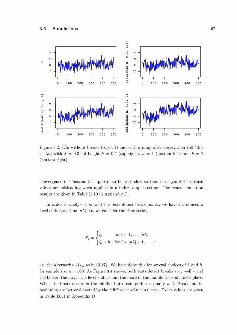
3.6 Simulations 67
x
0 100 200 300 400 500
-2
02
4
add.break(x, 0.3, 0.5)
0 100 200 300 400 500
-2
02
4
add.break(x, 0.3, 1)
0 100 200 300 400 500
-2
02
4
add.break(x, 0.3, 2)
0 100 200 300 400 500-2
02
4
Figure 3.2: fGn without breaks (top left) and with a jump after observation 150 (this
is [λn] with λ = 0.3) of height h = 0.5 (top right), h = 1 (bottom left) and h = 2
(bottom right).
convergence in Theorem 3.4 appears to be very slow so that the asymptotic critical
values are misleading when applied in a finite sample setting. The exact simulation
results are given in Table D.10 in Appendix D.
In order to analyze how well the tests detect break points, we have introduced a
level shift h at time [nλ], i.e. we consider the time series
Xi =
ξi for i = 1, . . . , [nλ]
ξi + h for i = [nλ] + 1, . . . , n,
i.e. the alternative Hλ,h as in (3.17). We have done this for several choices of λ and h,
for sample size n = 500. As Figure 3.4 shows, both tests detect breaks very well – and
the better, the larger the level shift is and the more in the middle the shift takes place.
When the break occurs in the middle, both tests perform equally well. Breaks at the
beginning are better detected by the “difference-of-means” test. Exact values are given
in Table D.11 in Appendix D.
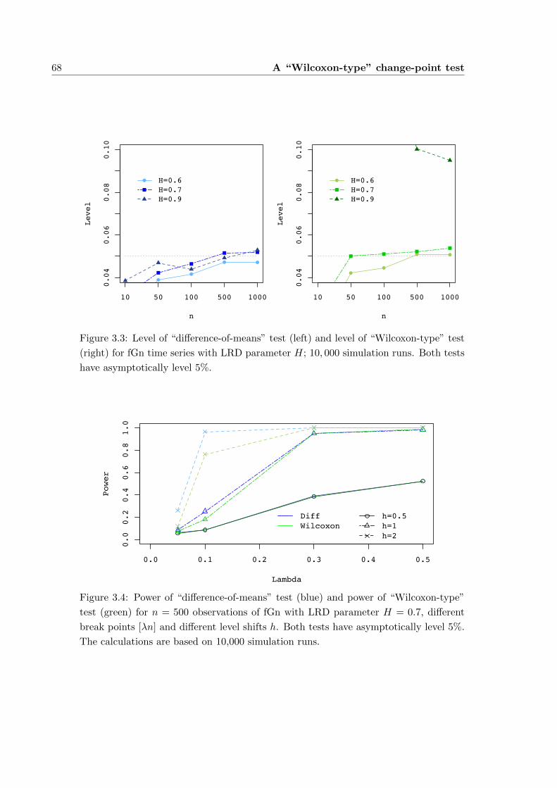
68 A “Wilcoxon-type” change-point test
0.04
0.06
0.08
0.10
n
Level
10 50 100 500 1000
H=0.6H=0.7H=0.9
0.04
0.06
0.08
0.10
n
Level
10 50 100 500 1000
H=0.6H=0.7H=0.9
Figure 3.3: Level of “difference-of-means” test (left) and level of “Wilcoxon-type” test
(right) for fGn time series with LRD parameter H; 10, 000 simulation runs. Both tests
have asymptotically level 5%.
0.0 0.1 0.2 0.3 0.4 0.5
0.0
0.2
0.4
0.6
0.8
1.0
Lambda
Power
h=0.5h=1h=2
DiffWilcoxon
Figure 3.4: Power of “difference-of-means” test (blue) and power of “Wilcoxon-type”
test (green) for n = 500 observations of fGn with LRD parameter H = 0.7, different
break points [λn] and different level shifts h. Both tests have asymptotically level 5%.
The calculations are based on 10,000 simulation runs.
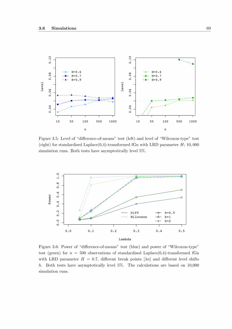
3.6 Simulations 69
0.04
0.06
0.08
0.10
n
Level
10 50 100 500 1000
H=0.6H=0.7H=0.9
0.04
0.06
0.08
0.10
n
Level
10 50 100 500 1000
H=0.6H=0.7H=0.9
Figure 3.5: Level of “difference-of-means” test (left) and level of “Wilcoxon-type” test
(right) for standardised Laplace(0,4)-transformed fGn with LRD parameter H; 10, 000
simulation runs. Both tests have asymptotically level 5%.
0.0 0.1 0.2 0.3 0.4 0.5
0.0
0.2
0.4
0.6
0.8
1.0
Lambda
Power
h=0.5h=1h=2
DiffWilcoxon
Figure 3.6: Power of “difference-of-means” test (blue) and power of “Wilcoxon-type”
test (green) for n = 500 observations of standardised Laplace(0,4)-transformed fGn
with LRD parameter H = 0.7, different break points [λn] and different level shifts
h. Both tests have asymptotically level 5%. The calculations are based on 10,000
simulation runs.

70 A “Wilcoxon-type” change-point test
0.06
0.08
0.10
0.12
0.14
n
Level
10 50 100 500 1000 2k 10k
H=0.6H=0.7H=0.9
0.06
0.08
0.10
0.12
0.14
n
Level
10 50 100 500 1000
H=0.6H=0.7H=0.9
Figure 3.7: Level of “difference-of-means” test (left) and level of “Wilcoxon-type” test
(right) for standardised Pareto(3,1)-transformed fGn with LRD parameter H; 10, 000
simulation runs. Both tests have asymptotically level 5%.
0.0 0.1 0.2 0.3 0.4 0.5
0.0
0.2
0.4
0.6
0.8
1.0
Lambda
Power
h=0.5h=1h=2
DiffWilcoxon
Figure 3.8: Power of “difference-of-means” test (blue) and power of “Wilcoxon-type”
test (green) for n = 500 observations of standardised Pareto(3,1)-transformed fGn with
LRD parameter H = 0.7, different break points [λn] and different level shifts h. Both
tests have asymptotically level 5%. The calculations are based on 10,000 simulation
runs.
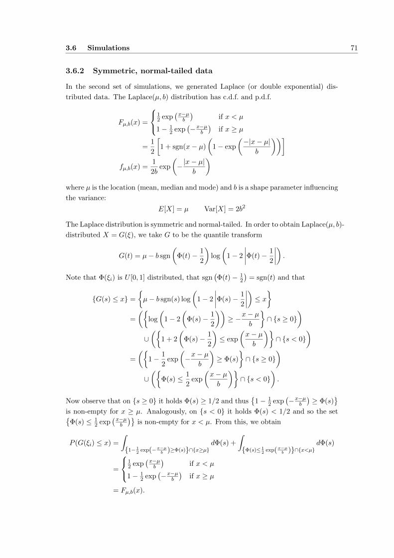
3.6 Simulations 71
3.6.2 Symmetric, normal-tailed data
In the second set of simulations, we generated Laplace (or double exponential) dis-
tributed data. The Laplace(µ, b) distribution has c.d.f. and p.d.f.
Fµ,b(x) =
12 exp
(x−µb
)if x < µ
1− 12 exp
(−x−µ
b
)if x ≥ µ
=1
2
[1 + sgn(x− µ)
(1− exp
(−|x− µ|
b
))]fµ,b(x) =
1
2bexp
(−|x− µ|
b
)where µ is the location (mean, median and mode) and b is a shape parameter influencing
the variance:
E[X] = µ Var[X] = 2b2
The Laplace distribution is symmetric and normal-tailed. In order to obtain Laplace(µ, b)-
distributed X = G(ξ), we take G to be the quantile transform
G(t) = µ− b sgn
(Φ(t)− 1
2
)log
(1− 2
∣∣∣∣Φ(t)− 1
2
∣∣∣∣) .Note that Φ(ξi) is U [0, 1] distributed, that sgn
(Φ(t)− 1
2
)= sgn(t) and that
G(s) ≤ x =
µ− b sgn(s) log
(1− 2
∣∣∣∣Φ(s)− 1
2
∣∣∣∣) ≤ x=
(log
(1− 2
(Φ(s)− 1
2
))≥ −x− µ
b
∩ s ≥ 0
)∪(
1 + 2
(Φ(s)− 1
2
)≤ exp
(x− µb
)∩ s < 0
)=
(1− 1
2exp
(−x− µ
b
)≥ Φ(s)
∩ s ≥ 0
)∪(
Φ(s) ≤ 1
2exp
(x− µb
)∩ s < 0
).
Now observe that on s ≥ 0 it holds Φ(s) ≥ 1/2 and thus
1− 12 exp
(−x−µ
b
)≥ Φ(s)
is non-empty for x ≥ µ. Analogously, on s < 0 it holds Φ(s) < 1/2 and so the set
Φ(s) ≤ 12 exp
(x−µb
)is non-empty for x < µ. From this, we obtain
P (G(ξi) ≤ x) =
∫1− 1
2exp(−x−µb )≥Φ(s)∩x≥µ
dΦ(s) +
∫Φ(s)≤ 1
2exp(x−µb )∩x<µ
dΦ(s)
=
12 exp
(x−µb
)if x < µ
1− 12 exp
(−x−µ
b
)if x ≥ µ
= Fµ,b(x).
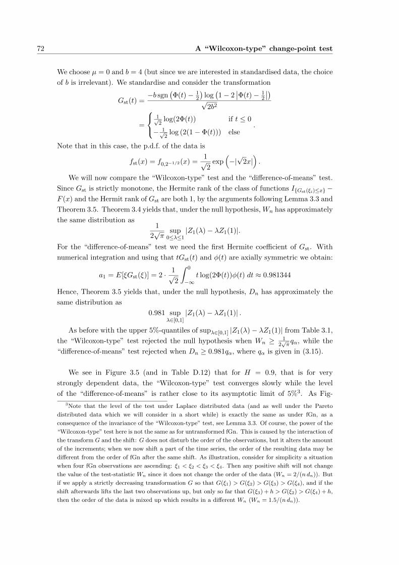
72 A “Wilcoxon-type” change-point test
We choose µ = 0 and b = 4 (but since we are interested in standardised data, the choice
of b is irrelevant). We standardise and consider the transformation
Gst(t) =−b sgn
(Φ(t)− 1
2
)log(1− 2
∣∣Φ(t)− 12
∣∣)√
2b2
=
1√2
log(2Φ(t)) if t ≤ 0
− 1√2
log (2(1− Φ(t))) else.
Note that in this case, the p.d.f. of the data is
fst(x) = f0,2−1/2(x) =1√2
exp(−|√
2x|).
We will now compare the “Wilcoxon-type” test and the “difference-of-means” test.
Since Gst is strictly monotone, the Hermite rank of the class of functions IGst(ξi)≤x−F (x) and the Hermit rank of Gst are both 1, by the arguments following Lemma 3.3 and
Theorem 3.5. Theorem 3.4 yields that, under the null hypothesis, Wn has approximately
the same distribution as1
2√π
sup0≤λ≤1
|Z1(λ)− λZ1(1)|.
For the “difference-of-means” test we need the first Hermite coefficient of Gst. With
numerical integration and using that tGst(t) and φ(t) are axially symmetric we obtain:
a1 = E[ξGst(ξ)] = 2 · 1√2
∫ 0
−∞t log(2Φ(t))φ(t) dt ≈ 0.981344
Hence, Theorem 3.5 yields that, under the null hypothesis, Dn has approximately the
same distribution as
0.981 supλ∈[0,1]
|Z1(λ)− λZ1(1)| .
As before with the upper 5%-quantiles of supλ∈[0,1] |Z1(λ)− λZ1(1)| from Table 3.1,
the “Wilcoxon-type” test rejected the null hypothesis when Wn ≥ 12√πqα, while the
“difference-of-means” test rejected when Dn ≥ 0.981qα, where qα is given in (3.15).
We see in Figure 3.5 (and in Table D.12) that for H = 0.9, that is for very
strongly dependent data, the “Wilcoxon-type” test converges slowly while the level
of the “difference-of-means” is rather close to its asymptotic limit of 5%3. As Fig-
3Note that the level of the test under Laplace distributed data (and as well under the Pareto
distributed data which we will consider in a short while) is exactly the same as under fGn, as a
consequence of the invariance of the “Wilcoxon-type” test, see Lemma 3.3. Of course, the power of the
“Wilcoxon-type” test here is not the same as for untransformed fGn. This is caused by the interaction of
the transform G and the shift: G does not disturb the order of the observations, but it alters the amount
of the increments; when we now shift a part of the time series, the order of the resulting data may be
different from the order of fGn after the same shift. As illustration, consider for simplicity a situation
when four fGn observations are ascending: ξ1 < ξ2 < ξ3 < ξ4. Then any positive shift will not change
the value of the test-statistic Wn since it does not change the order of the data (Wn = 2/(ndn)). But
if we apply a strictly decreasing transformation G so that G(ξ1) > G(ξ2) > G(ξ3) > G(ξ4), and if the
shift afterwards lifts the last two observations up, but only so far that G(ξ3) + h > G(ξ2) > G(ξ4) + h,
then the order of the data is mixed up which results in a different Wn (Wn = 1.5/(ndn)).
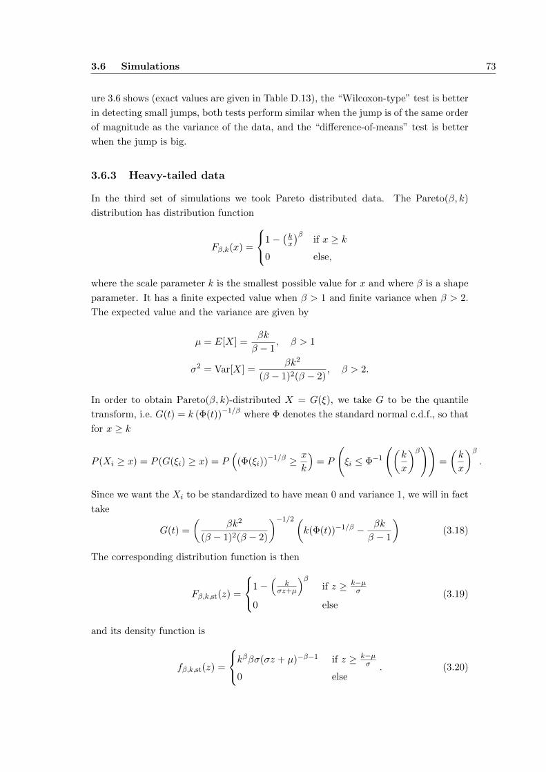
3.6 Simulations 73
ure 3.6 shows (exact values are given in Table D.13), the “Wilcoxon-type” test is better
in detecting small jumps, both tests perform similar when the jump is of the same order
of magnitude as the variance of the data, and the “difference-of-means” test is better
when the jump is big.
3.6.3 Heavy-tailed data
In the third set of simulations we took Pareto distributed data. The Pareto(β, k)
distribution has distribution function
Fβ,k(x) =
1−(kx
)βif x ≥ k
0 else,
where the scale parameter k is the smallest possible value for x and where β is a shape
parameter. It has a finite expected value when β > 1 and finite variance when β > 2.
The expected value and the variance are given by
µ = E[X] =βk
β − 1, β > 1
σ2 = Var[X] =βk2
(β − 1)2(β − 2), β > 2.
In order to obtain Pareto(β, k)-distributed X = G(ξ), we take G to be the quantile
transform, i.e. G(t) = k (Φ(t))−1/β where Φ denotes the standard normal c.d.f., so that
for x ≥ k
P (Xi ≥ x) = P (G(ξi) ≥ x) = P(
(Φ(ξi))−1/β ≥ x
k
)= P
(ξi ≤ Φ−1
((k
x
)β))=
(k
x
)β.
Since we want the Xi to be standardized to have mean 0 and variance 1, we will in fact
take
G(t) =
(βk2
(β − 1)2(β − 2)
)−1/2(k(Φ(t))−1/β − βk
β − 1
)(3.18)
The corresponding distribution function is then
Fβ,k,st(z) =
1−(
kσz+µ
)βif z ≥ k−µ
σ
0 else(3.19)
and its density function is
fβ,k,st(z) =
kββσ(σz + µ)−β−1 if z ≥ k−µσ
0 else. (3.20)
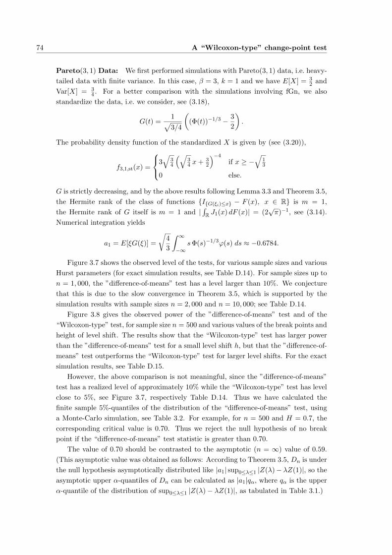
74 A “Wilcoxon-type” change-point test
Pareto(3, 1) Data: We first performed simulations with Pareto(3, 1) data, i.e. heavy-
tailed data with finite variance. In this case, β = 3, k = 1 and we have E[X] = 32 and
Var[X] = 34 . For a better comparison with the simulations involving fGn, we also
standardize the data, i.e. we consider, see (3.18),
G(t) =1√3/4
((Φ(t))−1/3 − 3
2
).
The probability density function of the standardized X is given by (see (3.20)),
f3,1,st(x) =
3√
34
(√34 x+ 3
2
)−4
if x ≥ −√
13
0 else.
G is strictly decreasing, and by the above results following Lemma 3.3 and Theorem 3.5,
the Hermite rank of the class of functions IG(ξi)≤x − F (x), x ∈ R is m = 1,
the Hermite rank of G itself is m = 1 and |∫R J1(x) dF (x)| = (2
√π)−1, see (3.14).
Numerical integration yields
a1 = E[ξG(ξ)] =
√4
3
∫ ∞−∞
sΦ(s)−1/3ϕ(s) ds ≈ −0.6784.
Figure 3.7 shows the observed level of the tests, for various sample sizes and various
Hurst parameters (for exact simulation results, see Table D.14). For sample sizes up to
n = 1, 000, the ”difference-of-means” test has a level larger than 10%. We conjecture
that this is due to the slow convergence in Theorem 3.5, which is supported by the
simulation results with sample sizes n = 2, 000 and n = 10, 000; see Table D.14.
Figure 3.8 gives the observed power of the ”difference-of-means” test and of the
“Wilcoxon-type” test, for sample size n = 500 and various values of the break points and
height of level shift. The results show that the “Wilcoxon-type” test has larger power
than the ”difference-of-means” test for a small level shift h, but that the ”difference-of-
means” test outperforms the “Wilcoxon-type” test for larger level shifts. For the exact
simulation results, see Table D.15.
However, the above comparison is not meaningful, since the ”difference-of-means”
test has a realized level of approximately 10% while the “Wilcoxon-type” test has level
close to 5%, see Figure 3.7, respectively Table D.14. Thus we have calculated the
finite sample 5%-quantiles of the distribution of the “difference-of-means” test, using
a Monte-Carlo simulation, see Table 3.2. For example, for n = 500 and H = 0.7, the
corresponding critical value is 0.70. Thus we reject the null hypothesis of no break
point if the “difference-of-means” test statistic is greater than 0.70.
The value of 0.70 should be contrasted to the asymptotic (n = ∞) value of 0.59.
(This asymptotic value was obtained as follows: According to Theorem 3.5, Dn is under
the null hypothesis asymptotically distributed like |a1| sup0≤λ≤1 |Z(λ)− λZ(1)|, so the
asymptotic upper α-quantiles of Dn can be calculated as |a1|qα, where qα is the upper
α-quantile of the distribution of sup0≤λ≤1 |Z(λ)− λZ(1)|, as tabulated in Table 3.1.)
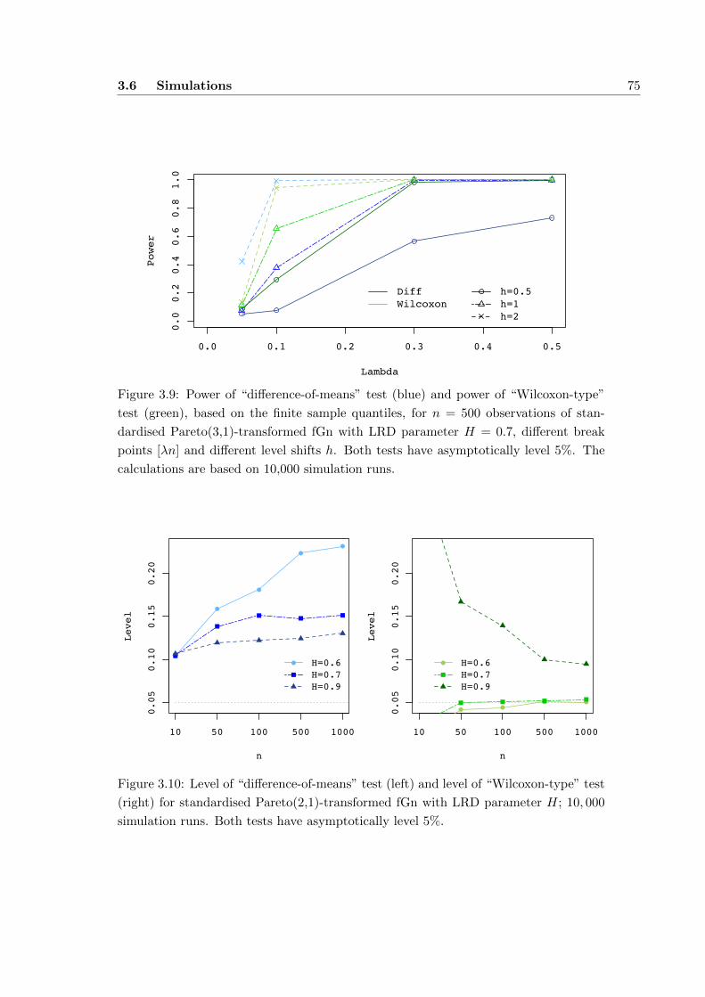
3.6 Simulations 75
0.0 0.1 0.2 0.3 0.4 0.5
0.0
0.2
0.4
0.6
0.8
1.0
Lambda
Power
h=0.5h=1h=2
DiffWilcoxon
Figure 3.9: Power of “difference-of-means” test (blue) and power of “Wilcoxon-type”
test (green), based on the finite sample quantiles, for n = 500 observations of stan-
dardised Pareto(3,1)-transformed fGn with LRD parameter H = 0.7, different break
points [λn] and different level shifts h. Both tests have asymptotically level 5%. The
calculations are based on 10,000 simulation runs.
0.05
0.10
0.15
0.20
n
Level
10 50 100 500 1000
H=0.6H=0.7H=0.9
0.05
0.10
0.15
0.20
n
Level
10 50 100 500 1000
H=0.6H=0.7H=0.9
Figure 3.10: Level of “difference-of-means” test (left) and level of “Wilcoxon-type” test
(right) for standardised Pareto(2,1)-transformed fGn with LRD parameter H; 10, 000
simulation runs. Both tests have asymptotically level 5%.
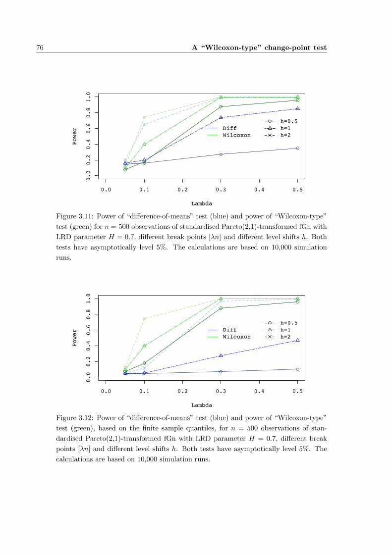
76 A “Wilcoxon-type” change-point test
0.0 0.1 0.2 0.3 0.4 0.5
0.0
0.2
0.4
0.6
0.8
1.0
Lambda
Power
h=0.5h=1h=2
DiffWilcoxon
Figure 3.11: Power of “difference-of-means” test (blue) and power of “Wilcoxon-type”
test (green) for n = 500 observations of standardised Pareto(2,1)-transformed fGn with
LRD parameter H = 0.7, different break points [λn] and different level shifts h. Both
tests have asymptotically level 5%. The calculations are based on 10,000 simulation
runs.
0.0 0.1 0.2 0.3 0.4 0.5
0.0
0.2
0.4
0.6
0.8
1.0
Lambda
Power
h=0.5h=1h=2
DiffWilcoxon
Figure 3.12: Power of “difference-of-means” test (blue) and power of “Wilcoxon-type”
test (green), based on the finite sample quantiles, for n = 500 observations of stan-
dardised Pareto(2,1)-transformed fGn with LRD parameter H = 0.7, different break
points [λn] and different level shifts h. Both tests have asymptotically level 5%. The
calculations are based on 10,000 simulation runs.
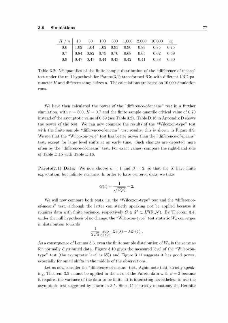
3.6 Simulations 77
H / n 10 50 100 500 1,000 2,000 10,000 ∞0.6 1.02 1.04 1.02 0.93 0.90 0.88 0.85 0.75
0.7 0.84 0.82 0.79 0.70 0.68 0.65 0.62 0.59
0.9 0.47 0.47 0.44 0.43 0.42 0.41 0.38 0.30
Table 3.2: 5%-quantiles of the finite sample distribution of the “difference-of-means”
test under the null hypothesis for Pareto(3,1)-transformed fGn with different LRD pa-
rameter H and different sample sizes n. The calculations are based on 10,000 simulation
runs.
We have then calculated the power of the ”difference-of-means” test in a further
simulation, with n = 500, H = 0.7 and the finite sample quantile critical value of 0.70
instead of the asymptotic value of 0.59 (see Table 3.2). Table D.16 in Appendix D shows
the power of the test. We can now compare the results of the “Wilcoxon-type” test
with the finite sample “difference-of-means” test results; this is shown in Figure 3.9.
We see that the “Wilcoxon-type” test has better power than the ”difference-of-means”
test, except for large level shifts at an early time. Such changes are detected more
often by the ”difference-of-means” test. For exact values, compare the right-hand side
of Table D.15 with Table D.16.
Pareto(2, 1) Data: We now choose k = 1 and β = 2, so that the X have finite
expectation, but infinite variance. In order to have centered data, we take
G(t) =1√Φ(t)
− 2.
We will now compare both tests, i.e. the “Wilcoxon-type” test and the “difference-
of-means” test, although the latter can strictly speaking not be applied because it
requires data with finite variance, respectively G ∈ G2 ⊂ L2(R,N ). By Theorem 3.4,
under the null hypothesis of no change, the “Wilcoxon-type” test statistic Wn converges
in distribution towards1
2√π
sup0≤λ≤1
|Z1(λ)− λZ1(1)|.
As a consequence of Lemma 3.3, even the finite sample distribution of Wn is the same as
for normally distributed data. Figure 3.10 gives the measured level of the “Wilcoxon-
type” test (the asymptotic level is 5%) and Figure 3.11 suggests it has good power,
especially for small shifts in the middle of the observations.
Let us now consider the “difference-of-means” test. Again note that, strictly speak-
ing, Theorem 3.5 cannot be applied in the case of the Pareto data with β = 2 because
it requires the variance of the data to be finite. It is interesting nevertheless to use the
asymptotic test suggested by Theorem 3.5. Since G is strictly monotone, the Hermite
78 A “Wilcoxon-type” change-point test
rank of G is m = 1 as well, by the Corollary following Theorem 3.5. Using numerical
integration, we have calculated
a1 = E [ξG(ξ)] =
∫ ∞−∞
s(Φ(s)−1/2 − 2)ϕ(s) ds =
∫ ∞−∞
sΦ(s)−1/2ϕ(s) ds ≈ −1.40861.
We clearly see in Figure 3.10 that the “difference-of-means” test very often falsely rejects
the null hypothesis, that is detects breaks where there are none, while the “Wilcoxon-
type” test is robust. Figure 3.11 shows that both tests have good power, but again, the
“Wilcoxon-type” test is clearly better, especially for small shifts in the middle of the
observations. For an exact comparison, see Table D.17 and Table D.15 in Appendix D.
As in the situation with Pareto(3,1) distributed data, the “difference-of-means”
test rejects the null hypothesis much too often (see Figure 3.10, it does not reach its
asymptotic level of 5%, it does not even seem to converge), so the power comparison is
again not meaningful.
So we have calculated the finite sample 5%-quantiles of the distribution of the
“difference-of-means” test here as well; the results are shown in Table D.16. Based
on these critical values, the test can be compared to the “Wilcoxon-type” test. In
this comparison, the “difference-of-means” test shows an even poorer performance, see
Figure 3.12.
Chapter 4
Power of some change-point tests
In Chapter 3, we have studied two tests for the change-point problem (H,A) as defined
in (3.1) and (3.2): The first test, the “Wilcoxon-type” test, rejects the null hypothesis
H for large values of the statistic
Wn =1
ndnmax
1≤k≤n−1
∣∣∣∣∣∣k∑i=1
n∑j=k+1
(IXi≤Xj −
1
2
)∣∣∣∣∣∣ , (4.1)
the second test, the “difference-of-means” test rejects H for large values of
Dn :=1
ndnmax
1≤k≤n−1
∣∣∣∣∣∣k∑i=1
n∑j=k+1
(Xj −Xi)
∣∣∣∣∣∣ . (4.2)
Note that for reasons of comparability, we like to define the kernel of Dn with a negative
sign here, in contrast to definition (3.16). In Chapter 3, we have derived the limit
distribution of both tests under the null hypothesis that no change occured and we
have simulated the behaviour of both tests under several alternatives (for data with a
jump in the mean of different heights and at various positions). Now we compute the
power of the above tests analytically under a local alternative. This chapter is based
on the article of Dehling, Rooch and Taqqu (2013).
We consider the following sequence of alternatives
Aτ,hn(n) : µi =
µ for i = 1, . . . , [nτ ]
µ+ hn for i = [nτ ] + 1, . . . , n,(4.3)
where 0 ≤ τ ≤ 1, in other words we consider a model where there is a jump of height hn
after a proportion of τ in the data. Note that the height hn of the level shift depends on
the sample size n; we will have to choose hn in a certain way to obtain a non-degenerate
limit distribution.

80 Power of some change-point tests
4.1 Power of the “difference-of-means” test under local
alternatives
We first investigate the asymptotic distribution of the process
Dn(λ) :=1
ndn
[nλ]∑i=1
n∑j=[nλ]+1
(Xj −Xi), 0 ≤ λ ≤ 1, (4.4)
under Aτ,hn(n), as defined in (4.3). Since the statistic Dn(λ) splits up the data into two
blocks at time [nλ] + 1, while the local alternative Aτ,hn(n) involves a jump at [nτ ] + 1,
we expect to obtain an interplay between λ and τ in the limit.
Under the general alternative A, as defined in (3.2), we obtain
Dn(λ) =1
ndn
[nλ]∑i=1
n∑j=[nλ]+1
(G(ξj)−G(ξi)) +1
ndn
[nλ]∑i=1
n∑j=[nλ]+1
(µj − µi), (4.5)
and under the local alternative Aτ,hn(n) (which is included in A), the second term is
1
ndn
[nλ]∑i=1
n∑j=[nλ]+1
(µj − µi) =
hnndn
[λn](n− [τn]) for λ ≤ τhnndn
(n− [λn])[τn] for λ ≥ τ.. (4.6)
We can write this in a shorter form, using the function δτ : [0, 1]→ R which we define
as
δτ (λ) =
λ(1− τ) for λ ≤ τ
(1− λ)τ for λ ≥ τ; (4.7)
note that δτ (λ) takes its maximum value τ(1− τ) at λ = τ . Now we obtain for large n
1
ndn
[nλ]∑i=1
n∑j=[nλ]+1
(µj − µi) ∼nhndn
δτ (λ).
Thus, in order for the second term in (4.5) to converge as n → ∞, we have to choose
the level shift hn ∼ c dn/n, where c is a constant. When n is large, this is exactly the
order of the level shift that can be detected with a non-trivial power (i.e. a power which
is neither 0 nor 1).
Theorem 4.1. Let G ∈ G2 be a transformation with Hermite rank m, as defined in
Section 1.4.2, and let (ξi)i≥1 be a stationary Gaussian process with mean zero, variance
1 and auto-covariance function as in (1.1) with 0 < D < 1m . For observations Xi =
µi +G(ξi), under the local alternative Aτ,hn(n) with
hn =dnnc (4.8)
4.1 “Differences-of-means” test 81
for an arbitrary constant c, the process (Dn(λ))0≤λ≤1 converges in distribution to the
processamm!
(λZm(1)− Zm(λ)) + c δτ (λ), (4.9)
where (Zm(λ))λ≥0 denotes the m-th order Hermite process with Hurst parameter H =
1 − Dm2 ∈ (1
2 , 1), and where am is the m-th Hermite coefficient of G, as defined in
Section 1.4.2.
Proof. We use decomposition (4.5). The first term on the right-hand side has the same
distribution as Dn(λ) under the null hypothesis, and thus it converges in distribution
to amm! (λZm(1) − Zm(λ)), see Theorem 3.5. Regarding the second term, we obtain by
(4.8) and (4.6)
1
ndn
[nλ]∑i=1
n∑j=[nλ]+1
(µj − µi) =
cn2 [λn](n− [τn]) for λ ≤ τcn2 (n− [λn])[τn] for λ ≥ τ.
→ c δτ (λ),
uniformly in λ ∈ [0, 1], as n→∞.
Remark. (i) For c = 0, which means hn = 0, the local alternative Aτ,hn(n) is identical
to the null hypothesis H, and in fact, Theorem 4.1 reproduces the limit distribution of
Dn under the null hypothesis. Thus, Theorem 4.1 is a generalization of Theorem 3.5.
(ii) Under the local alternative, i.e. when c 6= 0, the limit process is the sum of a
fractional bridge process (like in Theorem 3.1 and Theorem 3.5) and the deterministic
function c δτ .
(iii) As a corollary to Theorem 4.1, we can determine the asymptotic distribution of
test statistics based on the process (Dn(λ))0≤λ≤1 by applying the continuous mapping
theorem. For example, we get that Dn, as defined in (4.2) converges in distribution to
sup0≤λ≤1
|λZm(1)− Zm(λ) + c δτ (λ)|.
This limit distribution depends on the constant c. For c = 0, we obtain the limit
distribution under the null hypthesis, see Theorem 3.5. Increasing the value of |c| leads
to a shift of the distribution to the right.
(iv) For a given break position τ ∈ [0, 1], the function δτ (λ) takes its maximum value
in λ = τ , and this maximum value equals τ(1− τ). Thus, for values of τ close to 0 and
close to 1, τ(1− τ) is close to 0, and thus the effect of adding the term cδτ (λ) is rather
small. As a result, the power of the test is small at level shifts that occur very early or
very late in the process.
(v) The higher the level shift and the closer λ is to τ , the easier it is to detect the level
shift.
Theorem 4.1 can be applied in order to make power calculations for the change-
point test that rejects for large values of Dn. If we denote by qα the upper α-quantile
82 Power of some change-point tests
of the distribution of sup0≤λ≤1 |λZ(1) − Z(λ)|, where Z(λ) = Zm(λ)/m!, our test will
reject the null hypothesis H when Dn ≥ amqα, where am is the m-th Hermite coefficient
of G, see Theorem 3.5. By construction, this test has asymptotic level α, i.e. the test
rejects H with probability α if the null hypothesis H holds. If n is large and
h = hn =dnnc,
the power of the test at the alternative Aτ,h(n) is by (4.9) approximately given by
P
(sup
0≤λ≤1|λZm(1)− Zm(λ) + c δτ (λ)| ≥ qα
).
We may apply Theorem 4.1 as well in order to determine the size of a level shift at
time [τn] that can be detected with a given probability β. To this end, we calculate c
such that
P
(sup
0≤λ≤1|λZm(1)− Zm(λ) + c δτ (λ)| ≥ qα
)= β.
Choosing then h = dnn c, we get that the asymptotic power of the test at the alternative
Aτ,h(n) is equal to β. Thus, a level shift of this size can be detected with probability
β with a test that has level α.
4.2 Power of the “Wilcoxon-type” test under local alter-
natives
Theorem 4.2. Suppose that (ξi)i≥1 is a stationary Gaussian process with mean zero,
variance 1 and auto-covariance function (1.1) with 0 ≤ D < 1m . Moreover, let G ∈ G1,
and assume that G(ξi) has continuous distribution function F (x). Let m denote the
Hermite rank of the class of functions IG(ξi)≤x−F (x), x ∈ R. Then, under Aτ,hn, as
defined in (4.3), if hn → 0 as n→∞
1
ndn
[nλ]∑i=1
n∑j=[nλ]+1
(IXi≤Xj −
1
2
)− n
dnδτ (λ)
∫R
(F (x+ hn)− F (x)) dF (x), (4.10)
indexed by 0 ≤ λ ≤ 1, converges in distribution towards the process
1
m!(Zm(λ)− λZm(1))
∫RJm(x) dF (x), 0 ≤ λ ≤ 1,
where (Zm(λ))λ≥0 denotes the m-th order Hermite process with Hurst parameter H =
1− Dm2 ∈ (1
2 , 1) and where Jm(x) = E[Hm(ξi)IG(ξi)≤x
].
Remark. (i) Note that we make no assumption about the exact order of the sequence
(hn)n≥1. Theorem 4.2 holds under the very general assumption that hn → 0 as n→∞.
4.2 “Wilcoxon-type” test 83
(ii) If we choose (hn)n≥1 as in (4.8), the centering constants in (4.10) converge, provided
some technical assumptions are satisfied. To see this, observe that
n
dnδτ (λ)
∫R
(F (x+ hn)− F (x)) dF (x) =nhndn
δτ (λ)
∫R
F (x+ hn)− F (x)
hndF (x)
→ c δτ (λ)
∫Rf(x) dF (x)
= c δτ (λ)
∫Rf2(x) dx.
The convergence in the next to last step requires some justification; it holds for example
if F is differentiable with bounded derivative f(x).
Corollary. Suppose that (ξi)i≥1 is a stationary Gaussian process with mean zero, vari-
ance 1 and auto-covariance function as in (1.1) with 0 ≤ D < 1m . Moreover, let G ∈ G1,
and assume that G(ξk) has a distribution function F (x) with bounded density f(x). Let
m denote the Hermite rank of the class of functions IG(ξi)≤x − F (x), x ∈ R. Then,
under the sequence of alternatives Aτ,hn, as defined in (4.3), with hn = cdnn we obtain
that
1
ndn
[nλ]∑i=1
n∑j=[nλ]+1
(IXi≤Xj −
1
2
)(4.11)
converges in distribution to the process
1
m!(Zm(λ)− λZm(1))
∫RJm(x) dF (x) + cδτ (λ)
∫Rf2(x) dx, 0 ≤ λ ≤ 1.
Proof of Theorem 4.2. We use the same techniques as in the proof of Theorem 3.1,
where we derived the limit distribution of the “Wilcoxon-type” test statistic under the
null hypothesis; more precisely we will decompose the test statistic (4.10) into a term
whose distribution is the same both under the null hypothesis as well as under the
alternative, and a second term which, after proper centering, converges to zero.
We express our test statistic as a functional of the e.d.f. Fk(x) of the first k ob-
servations G(ξ1), . . . , G(ξk) and of the e.d.f. Fk,l(x) which is based on the observations
G(ξk), . . . , G(ξl). Recall that under the local alternative, we have
Xi =
G(ξi) + µ for i = 1, . . . , [nτ ]
G(ξi) + µ+ hn for i = [nτ ] + 1, . . . , n.
84 Power of some change-point tests
Thus we obtain for λ ≤ τ[nλ]∑i=1
n∑j=[nλ]+1
IXi≤Xj
=
[nλ]∑i=1
[nτ ]∑j=[nλ]+1
IG(ξi)+µ≤G(ξj)+µ +
[nλ]∑i=1
n∑j=[nτ ]+1
IG(ξi)+µ≤G(ξj)+µ+hn
=
[nλ]∑i=1
[nτ ]∑j=[nλ]+1
IG(ξi)≤G(ξj) +
[nλ]∑i=1
n∑j=[nτ ]+1
IG(ξi)≤G(ξj)+hn
=
[nλ]∑i=1
n∑j=[nλ]+1
IG(ξi)≤G(ξj) +
[nλ]∑i=1
n∑j=[nτ ]+1
(IG(ξi)≤G(ξj)+hn − IG(ξi)≤G(ξj)
)
=
[nλ]∑i=1
n∑j=[nλ]+1
IG(ξi)≤G(ξj) +
[nλ]∑i=1
n∑j=[nτ ]+1
IG(ξj)<G(ξi)≤G(ξj)+hn. (4.12)
In the same way, we obtain for λ ≥ τ[nλ]∑i=1
n∑j=[nλ]+1
IXi≤Xj
=
[nτ ]∑i=1
n∑j=[nλ]+1
IG(ξi)+µ≤G(ξj)+µ+hn +
[nλ]∑i=[nτ ]+1
n∑j=[nλ]+1
IG(ξi)+µ+hn≤G(ξj)+µ+hn
=
[nτ ]∑i=1
n∑j=[nλ]+1
IG(ξi)≤G(ξj)+hn +
[nλ]∑i=[nτ ]+1
n∑j=[nλ]+1
IG(ξi)≤G(ξj)
=
[nλ]∑i=1
n∑j=[nλ]+1
IG(ξi)≤G(ξj) +
[nτ ]∑i=1
n∑j=[nλ]+1
(IG(ξi)≤G(ξj)+hn − IG(ξi)≤G(ξj)
)
=
[nλ]∑i=1
n∑j=[nλ]+1
IG(ξi)≤G(ξj) +
[nτ ]∑i=1
n∑j=[nλ]+1
IG(ξj)<G(ξi)≤G(ξj)+hn. (4.13)
We recognize that for the first term on the right-hand side of (4.12) and (4.13), we each
get the asymptotic distribution via Theorem 3.1. Thus, in order to prove Theorem 4.2,
it suffices to show that the following two terms,
1
ndnsup
0≤λ≤τ
∣∣∣∣∣∣[nλ]∑i=1
n∑j=[nτ ]+1
IG(ξj)<G(ξi)≤G(ξj)+hn − n2λ(1−τ)
∫R
(F (x+ hn)−F (x)) dF (x)
∣∣∣∣∣∣(4.14)
and
1
ndnsupτ≤λ≤1
∣∣∣∣∣∣[nτ ]∑i=1
n∑j=[nλ]+1
IG(ξj)<G(ξi)≤G(ξj)+hn − n2τ(1−λ)
∫R
(F (x+ hn)−F (x)) dF (x)
∣∣∣∣∣∣(4.15)

4.2 “Wilcoxon-type” test 85
both converge to zero in probability. We first show this for (4.14). Observe that
[nλ]∑i=1
n∑j=[nτ ]+1
IG(ξj)<G(ξi)≤G(ξj)+hn − n2λ(1− τ)
∫R
(F (x+ hn)− F (x)) dF (x)
= [nλ]n∑
j=[nτ ]+1
(F[nλ](G(ξj) + hn)− F[nλ](G(ξj))
)− n2λ(1− τ)
∫R
(F (x+ hn)− F (x)) dF (x)
= [nλ](n−[nτ ])
∫R
(F[nλ](x+ hn)− F[nλ](x)
)dF[nτ ]+1,n(x)
− n2λ(1− τ)
∫R
(F (x+ hn)− F (x)) dF (x)
= [nλ](n−[nτ ])(∫
R(F[nλ](x+ hn)− F[nλ](x)) dF[nτ ]+1,n(x)
−∫R
(F (x+ hn)− F (x)) dF (x))
+([nλ](n− [nτ ])− n2λ(1− τ)
) ∫R
(F (x+ hn)− F (x)) dF (x).
Note that by the basic estimate nλ− 1 ≤ [nλ] ≤ nλ+ 1 we obtain
[nλ](n− [nτ ])− n2λ(1− τ)
= [nλ]n(1− τ) + [nλ](n− [nτ ]− n(1− τ))− n2λ(1− τ)
= nλn(1− τ) + n(1− τ) ([nλ]− nλ) + [nλ] (n− [nτ ]− n(1− τ))− n2λ(1− τ)
= [nλ] (nτ − [nτ ]) + (1− τ)n ([nλ]− nλ)
≤ [nλ] + (1− τ)n = O(n).
Together with |∫R(F (x+ hn)− F (x))dF (x)| ≤ 1, this yields
1
ndn
([nλ](n− [nτ ])− n2λ(1− τ)
) ∫R
(F (x+ hn)− F (x)) dF (x) = O
(1
dn
)→ 0,
as n → ∞. Hence, in order to show that (4.14) converges to zero in probability, it
suffices to show that
[nλ](n− [nτ ])
ndn
(∫R
(F[nλ](x+ hn)− F[nλ](x))dF[nτ ]+1,n(x)−∫R
(F (x+ hn)− F (x))dF (x)
)(4.16)

86 Power of some change-point tests
converges to zero in probability. In order to prove this, we rewrite the difference of the
integrals in (4.16) as
∫R
(F[nλ](x+ hn)− F[nλ](x)
)dF[nτ ]+1,n(x)−
∫R
(F (x+ hn)− F (x)) dF (x) (4.17)
=
∫R
(F[nλ](x+ hn)− F[nλ](x)
)− (F (x+ hn)− F (x)) dF[nτ ]+1,n(x)
+
∫R
(F (x+ hn)− F (x)) d(F[nτ ]+1,n − F )(x)
=
∫R
(F[nλ](x+ hn)− F[nλ](x)
)− (F (x+ hn)− F (x)) dF[nτ ]+1,n(x)
−∫R
(F[nτ ]+1,n(x)− F (x)
)d(F (x+ hn)− F (x)),
where we have used integration by parts in the final step. Thus, in order to prove that
(4.16) converges to zero, it suffices to show that the following two terms converge in
probability, as n→ 0,
1
dn[nλ]
∫R
((F[nλ](x+ hn)− F[nλ](x))− (F (x+ hn)− F (x))
)dF[nτ ]+1,n(x)→ 0 (4.18)
1
dn(n− [nτ ])
∫R
(F[nτ ]+1,n(x)− F (x)
)d(F (x+ hn)− F (x))→ 0.
(4.19)
In order to prove (4.18) and (4.19), we now employ the empirical process non-central
limit theorem (3.8), just like in the proof for the limit under the null hypothesis. Note
that by definition of the e.d.f., for any λ ≤ τ
([nτ ]− [nλ])(F[nλ]+1,[nτ ](x)− F (x)) = [nτ ](F[nτ ](x)− F (x))− [nλ](F[nλ](x)− F (x)).
Hence, we may deduce from (3.8) the following limit theorem for the e.d.f. of the
observations X[nλ]+1, . . . , X[nτ ],
sup0≤λ≤τ, x∈R
∣∣d−1n ([nτ ]− [nλ])(F[nλ]+1,[nτ ](x)− F (x))− J(x)(Z(τ)− Z(λ))
∣∣→ 0, (4.20)
almost surely. For τ = 1, this is
sup0≤λ≤1, x∈R
∣∣d−1n (n− [nλ])(F[nλ]+1,n − F (x))− J(x)(Z(1)− Z(λ))
∣∣→ 0, (4.21)
4.2 “Wilcoxon-type” test 87
almost surely. Now we return to (4.18), which is to show, and write∣∣∣∣∫R
1
dn[nλ]
((F[nλ](x+ hn)− F[nλ](x))− (F (x+ hn)− F (x))
)dF[nτ ]+1,n(x)
∣∣∣∣ (4.22)
≤∣∣∣∣∫
R(J(x+ hn)− J(x))Z(λ) dF[nτ ]+1,n(x)
∣∣∣∣+ supx∈R,0≤λ≤1
∣∣∣∣ 1
dn[nλ]
((F[nλ](x+ hn)− F[nλ](x))− (F (x+ hn)− F (x))
)− (J(x+ hn)− J(x))Z(λ)
∣∣∣∣≤∣∣∣∣∫
R(J(x+ hn)− J(x)) dF[nτ ]+1,n(x)
∣∣∣∣ sup0≤λ≤1
|Z(λ)|
+ supx∈R,0≤λ≤1
∣∣∣∣ 1
dn[nλ]
((F[nλ](x+ hn)− F[nλ](x))− (F (x+ hn)− F (x))
)− (J(x+ hn)− J(x))Z(λ)
∣∣∣∣.The second term on the right-hand side converges to zero by (3.8). Concerning the first
term, note that
J(x) =
∫RIG(y)≤xHm(y)ϕ(y) dy = −
∫RIx≤G(y)Hm(y)ϕ(y) dy, (4.23)
where ϕ(y) = 1√2πe−y
2/2 denotes the standard normal density function. For the second
identity, we have used the fact that G(ξ), by assumption, has a continuous distribution
and that∫RHm(y)ϕ(y) dy = 0 for m ≥ 1. Using (4.23), we thus obtain∫
RJ(x) dF[nτ ]+1,n(x) = −
∫R
∫RIx≤G(y)Hm(y)ϕ(y) dy dF[nτ ]+1,n(x) (4.24)
= −∫R
(∫RIx≤G(y) dF[nτ ]+1,n(x)
)Hm(y)ϕ(y) dy
= −∫RF[nτ ]+1,n(G(y))Hm(y)ϕ(y) dy,
and, using analogous arguments,∫RJ(x+ hn) dF[nτ ]+1,n(x) = −
∫RF[nτ ]+1,n(G(y)− hn)Hm(y)ϕ(y) dy. (4.25)
By the Glivenko-Cantelli theorem, applied to the stationary, ergodic process (G(ξi))i≥1,
we get supx∈R |Fn(x)− F (x)| → 0, almost surely. Since
F[nτ ]+1,n(x) =n
n− [nτ ]Fn(x)− [nτ ]
n− [nτ ]F[nτ ](x),
and thus∣∣F[nτ ]+1,n(x)− F (x)∣∣ ≤ ∣∣∣∣ n
n− [nτ ](Fn(x)− F (x))
∣∣∣∣+
∣∣∣∣ [nτ ]
n− [nτ ](F[nτ ](x)− F (x))
∣∣∣∣+
∣∣∣∣( [nτ ]
n− [nτ ]− n
n− [nτ ]
)F (x) + F (x)
∣∣∣∣ ,

88 Power of some change-point tests
we get that, almost surely,
supx∈R
∣∣F[nτ ]+1,n(x)− F (x)∣∣→ 0. (4.26)
Returning to the first term on the right-hand side of (4.22), we obtain, using (4.24)
and (4.25), ∣∣∣∣∫R
(J(x+ hn)− J(x)) dF[nτ ]+1,n(x)
∣∣∣∣=
∣∣∣∣∫R
(F[nτ ]+1,n(G(y)− hn)− F[nτ ]+1,n(G(y))
)Hm(y)ϕ(y) dy
∣∣∣∣≤∫R|F (G(y)− hn)− F (G(y))| |Hm(y)|ϕ(y) dy
+ 2 supx
∣∣F[nτ ]+1,n(x)− F (x)∣∣ ∫
R|Hm(y)|ϕ(y) dy.
Both terms on the right-hand side converge to zero; the second one by (4.26), the
first one by continuity of F and Lebesgue’s dominated convergence theorem, since F is
bounded by 1. In both cases, we have made use of the fact that∫|Hm(y)|ϕ(y) dy <∞.
Thus we have finally established (4.18). In order to prove (4.19), we observe that
1
dn(n− [nτ ])
∫R
(F[nτ ]+1,n(x)− F (x)
)d(F (x+ hn)− F (x))
≤∣∣∣∣∫
RJ(x)(Z(1)− Z(τ))d(F (x+ hn)− F (x))
∣∣∣∣+ supx∈R
∣∣∣∣ 1
dn(n− [nτ ])(F[nτ ]+1,n(x)− F (x))− J(x)(Z(1)− Z(τ))
∣∣∣∣≤∣∣∣∣∫
RJ(x) d(F (x+ hn)− F (x))
∣∣∣∣ |Z(1)− Z(τ)|
+ supx∈R
∣∣∣∣ 1
dn(n− [nτ ])(F[nτ ]+1,n(x)− F (x))− J(x)(Z(1)− Z(τ))
∣∣∣∣ .The second term on the right-hand side converges to zero by (4.21). Concerning the
first term, note that∫RJ(x) d(F (x+ hn)− F (x)) = E [J(G(ξi)− hn)− J(G(ξi))] .
Applying Lebesgue’s dominated convergence theorem and making use of the fact that,
by assumption, J is continuous, we obtain that∫R J(x) d(F (x + hn) − F (x)) → 0. In
this way, we have finally proved that (4.14) converges to zero, in probability. By similar
arguments, we can prove this for (4.15), which finally ends the proof of Theorem 4.2.
4.3 Asymptotic Relative Efficiency
In this section, we calculate the asymptotic relative efficiency (ARE) of the “Wilcoxon-
type” test, based on (4.1), over the “difference-of-means” test, based on (4.2). To do
4.3 Asymptotic Relative Efficiency 89
so, we calculate the number of observations needed to detect a small level shift h at
time [τn] with a test of given (asymptotic) level α and given (asymptotic) power β,
both for the “Wilcoxon-type” test and the “difference-of-means” test, and denote these
numbers by nW and nD, respectively. We then define the asymptotic relative efficiency
of the “Wilcoxon-type” test over the “difference-of-means” test by
ARE(W,D) = limh→0
nDnW
. (4.27)
It will turn out that this limit exists and that the ARE does not depend on the choice
of τ, α, β. An ARE less than 1 means that the “Wilcoxon-type” test needs on large
scale more observations than the “difference-of-means” test in order to detect a given
jump on the same level with the same power; this is what we call less efficient.
As preparation, we first calculate a quantity that is related to the ARE, namely the
ratio of the sizes of level shifts that can be detected by the two tests, based on the same
number of observations n, again for given values of τ, α, β. We denote the corresponding
level shifts by hW (n) and hD(n), respectively, assuming that these numbers depend on
n in the following way
hW (n) = cWdnn
hD(n) = cDdnn,
as specified in Theorem 4.1 and Theorem 4.2. In order to simplify the following con-
siderations, we take a one-sided change-point test, thus rejecting the hypothesis of no
change-point for large values of
max1≤k≤n−1
k∑i=1
n∑j=k+1
(Xj −Xi)
and
max1≤k≤n−1
k∑i=1
n∑j=k+1
IXi≤Xj,
respectively. These are the appropriate tests when testing against the alternative of
a non-negative level shift. In order to obtain tests that have asymptotically level α,
the “difference-of-means” test and the “Wilcoxon-type” test reject the null hypothesis
when the test statistics
m!
ndn ammax
1≤k≤n−1
k∑i=1
n∑j=k+1
(Xj −Xi) (4.28)
and
m!
ndn∫R Jm(x)dF (x)
max1≤k≤n−1
k∑i=1
n∑j=k+1
(IXi≤Xj −
1
2
)(4.29)
90 Power of some change-point tests
exceed the upper α quantile qα of the distribution of sup0≤λ≤1(Zm(λ) − λZm(1)), see
Theorem 3.5 and Theorem 3.1 and keep in mind that we changed the sign of the kernel of
the “difference-of-means” test statistic here. Under the sequence of alternatives Aτ,hD(n)
and Aτ,hW (n), respectively, the asymptotic distribution of the above test statistics is
given by
sup0≤λ≤1
(Zm(λ)− λZm(1) +
cDm!
amδτ (λ)
)and
sup0≤λ≤1
(Zm(λ)− λZm(1) +
cW m!∫f2(x)dx∫
R Jm(x)dF (x)δτ (λ)
),
respectively, see Theorem 4.1 and Theorem 4.2 (or Corollary 4.2). Thus, the asymptotic
power of these tests, based on (4.28) and (4.29), is given by the following formulae,
P
(sup
0≤λ≤1
(Zm(λ)− λZm(1) +
cDm!
amδτ (λ)
)≥ qα
)(4.30)
and
P
(sup
0≤λ≤1
(Zm(λ)− λZm(1) +
cW m!∫f2(x)dx∫
R Jm(x)dF (x)δτ (λ)
)≥ qα
). (4.31)
Thus, if we want the two tests to have identical power, we have to choose cD and cW
in such a way thatcDm!
amδτ (λ) =
cW m!∫f2(x)dx∫
R Jm(x)dF (x)δτ (λ),
which yields
hD(n)
hW (n)=cDcW
=am∫R f
2(x)dx∫R Jm(x)dF (x)
.
This quantity gives the ratio of the height of a level shift that can be detected by a
“difference-of-means” test over the height that can be detected by a “Wilcoxon-type”
test, when both tests are assumed to have the same level α, the same power β and the
shifts are taking place at the same time [nτ ]. In addition, we assume that the tests are
based on the same number of observations n, which is supposed to be large.
Example. For the case of Gaussian data, i.e. when G(t) = t, we have m = 1, a1 = −1
(the minus sign arises because we consider for the “difference-of-means” test statistic
the kernel y− x, instead of x− y like in Section 3.4.2) and∫R J1(x)dF (x) = − 1
2√π
, see
(3.14). Thus we obtain
hD(n)
hW (n)=cDcW
= 2√π
∫R
1
2πe−x
2dx =
∫R
1√πe−x
2dx = 1. (4.32)
Hence, both tests can asymptotically, as n→∞, detect level shifts of the same height.
This is surprising, because according to conventional statistical wisdom, a Gauß-type
test such as the “difference-of-means” test should outperform a rank test when the
underlying data have a normal distribution; this is at least the case for independent
observations.

4.3 Asymptotic Relative Efficiency 91
In order to calculate the ARE now, we need to consider the ratio of the sample sizes
nW and nD corresponding to a given level shift hn. We will thus study the probability
ψ(t) := P
(sup
0≤λ≤1(Zm(λ)− λZm(1) + t δτ (λ)) ≥ qα
)as a function of t, for fixed values of τ and α. The function ψ is monotonically increasing.
We define the generalized inverse
ψ−(β) := inft ≥ 0 : ψ(t) ≥ β.
Thus, we get
P
(sup
0≤λ≤1
(Zm(λ)− λZm(1) + ψ−(β) δτ (λ)
)≥ qα
)≥ β, (4.33)
and, in fact, for given τ , α and β, ψ−(β) is the smallest number having this property.
With the help of the function ψ−(β), we can apply Theorem 4.1 and Theorem 4.2
in order to calculate the number of observations needed to detect a level shift of a given
height. By comparing (4.30) and (4.33), we can detect a level shift of size h at time
[nτ ] with the “difference-of-means” test of (asymptotic) level α and power β based on
n observations, if hD(n) = dnn cD, where cD satisfies cDm!
am= ψ−(β). Hence we obtain
that hD(n) has to satisfy
hD(n) =dnn
amm!
ψ−(β).
Similarly, by comparing (4.31) and (4.33), we get for the “Wilcoxon-type” test that n
has to satisfy
hW (n) =dnn
∫R Jm(x) dF (x)
m!∫R f
2(x) dxψ−(β).
Solving these two equations for n and denoting the resulting numbers of observations
by nD and nW , respectively, we obtain
nD =
(hDm!
ψ−(β)Lm/2(n)am
)−2/Dm
nW =
(hW m!
∫R f
2(x) dx
ψ−(β)Lm/2(n)∫R Jm(x) dF (x)
)−2/Dm
,
and thus we have established the following theorem.
Theorem 4.3. Suppose that (ξi)i≥1 is a stationary Gaussian process with mean zero,
variance 1 and auto-covariance function (1.1) with 0 ≤ D < 1m . Moreover, let G ∈ G2,
and assume that G(ξi) has continuous distribution function F (x). Let m denote the
Hermite rank of the class of functions IG(ξi)≤x −F (x), x ∈ R. Then, the ARE of the
“Wilcoxon-type” test over the “difference-of-means” test, as defined in (4.27), is given
by
ARE(W,D) =
(am
∫R f
2(x)dx∫R Jm(x)dF (x)
)2/Dm
. (4.34)

92 Power of some change-point tests
Here, am is the m-th Hermite coefficient of G(·), as defined in Section 1.4.2, and Jm(x)
is the m-th Hermite coefficient of the class IG(·)≤x − F (x), x ∈ R. The “Wilcoxon-
type” test and the “difference-of-means” test are based on (4.28) and (4.29), respec-
tively.
Example. (i) In the case of Gaussian observations, i.e. G(t) = t, we have m = 1,
a1 = −1, f(x) = ϕ(x) = (2π)−1/2e−x2/2 and
∫R J(x) dF (x) = −(2
√π)−1, like in (3.14),
so after all we obtain
ARE(W,D) = 1.
(ii) When we consider the transformation
G(t) =1√3/4
((Φ(t))−1/3 − 3
2
),
we obtain, according to Section 3.6.3, standardized Pareto(3,1) data with p.d.f. and
c.d.f.
f3,1,st(x) =
3√
34
(√34 x+ 3
2
)−4
if x ≥ −√
13
0 else
and
F3,1,st(x) =
1−(
1√3/4t+3/2
)3
t ≥ 1−3/2√3/4
0 else
,
and the Hermite rank m equals 1. With numerical integration we obtain
ARE(W,D) ≈ (−2.678)2/D .
We will illustrate these findings by a set of computer simulations in Section 4.6.
4.4 ARE for i.i.d. data
We have shown that in the case of LRD data, the ARE of the “Wilcoxon-type” test and
the “difference-of-means” test is 1 for Gaussian data. In this section, we will compare
this surprising result with the case of i.i.d. Gaussian data. We will find that in this
case, the ARE is 3π , i.e. the “Wilcoxon-type” test is less efficient than the “difference-
of-means” test.
We consider i.i.d. observations X1, . . . , Xn with Xi ∼ N (0, 1) and the U -statistic
Uk =
k∑i=1
n∑j=k+1
h(Xi, Xj).
4.4 ARE for i.i.d. data 93
As kernel we will choose hD(x, y) = y − x and hW (x, y) = Ix≤y − 12 , in other words
we consider
U(D)k =
k∑i=1
n∑j=k+1
hD(Xi, Xj) =k∑i=1
n∑j=k+1
(Xj −Xi),
U(W )k =
k∑i=1
n∑j=k+1
hW (Xi, Xj) =
k∑i=1
n∑j=k+1
(IXi≤Xj −
1
2
).
Both kernels hD, hW are antisymmetric, i.e. they satisfy h(x, y) = −h(y, x), so in order
to determine the limit behaviour of U(D)k and U
(W )k , we can apply the limit theorems
of Csorgo and Horvath (1988).
Theorem 4.4. Let X1, . . . , Xn be i.i.d. random variables with Xi ∼ N (0, 1). Under
the null hypothesis of no change in the mean, it holds
sup0≤λ≤1
∣∣∣∣ 1
n3/2U
(D)[λn] − BB1,n(λ)
∣∣∣∣ = oP (1) (4.35)
and
sup0≤λ≤1
∣∣∣∣∣∣ 1
n3/2√
112
U(W )[λn] − BB2,n(λ)
∣∣∣∣∣∣ = oP (1), (4.36)
where (BBi,n(λ))0≤λ≤1, i = 1, 2, is a sequence of Brownian bridges with mean E[BBi,n(λ)] =
0 and auto-covariance E[BBi,n(s) BBi,n(t)] = min(s, t)− st.
Proof. By Theorem 4.1 of Csorgo and Horvath (1988), it holds under the null hypothesis
H that
sup0≤λ≤1
∣∣∣∣ 1
n3/2σU[λn] − BBn(λ)
∣∣∣∣ = oP (1)
where (BBn(λ))0≤λ≤1 is a sequence of Brownian bridges like BB1,n and BB2,n above
and where σ2 = E[h2(X1)] with h(t) = E[h(t,X1)]. The kernel h has to fulfill
E[h2(X1, X2)] < ∞ which is the case for hD(x, y) = y − x and hW (x, y) = Ix≤y − 12
and Gaussian Xi.
Theorem 4.5. Let X1, . . . , Xn be i.i.d. random variables with Xi ∼ N (0, 1). Under
the sequence of alternatives Aτ,hn(n), as defined in (4.3), and with hn = 1√nc, where c
is a constant, it holds(1
n3/2U
(D)[λn]
)0≤λ≤1
→ (BB1(λ) + cδτ (λ))0≤λ≤1 (4.37)
94 Power of some change-point tests
and
1
n3/2√
112
U(W )[λn]
0≤λ≤1
→
BB2(λ) +c
2√π ·√
112
δτ (λ)
0≤λ≤1
(4.38)
in distribution, where (BBi(λ))0≤λ≤1 is a Brownian bridge, i = 1, 2, and δτ (λ) is defined
in (4.7).
Proof. First, we prove (4.37). Like for the case of LRD observations, we decompose
the statistic, so that we obtain under the sequence of alternatives Aτ,hn(n)
1
n3/2U
(D)[λn] =
1
n3/2
[λn]∑i=1
n∑j=[λn]+1
(εj − εi) +1
n3/2
[λn]∑i=1
n∑j=[λn]+1
(µj − µi).
By Theorem 4.4, the first term on the right-hand side converges to a Brownian bridge
BB(λ). For the second term we have like in the proof for LRD observations
1
n3/2
[λn]∑i=1
n∑j=[λn]+1
(µj − µi) ∼√nhnδτ (λ),
and in order for the right-hand side to converge, we have to choose hn = 1√nc.
Now prove (4.38). Again like for LRD observations, we decompose the statistic into
one term that converges like under the null hypothesis and one term which converges
to a constant. Under the sequence of alternatives Aτ,hn(n) and for the case λ ≤ τ , this
decomposition is
1
n3/2U
(W )[λn] =
1
n3/2
[λn]∑i=1
n∑j=[λn]+1
(Iεi≤εj −
1
2
)+
1
n3/2
[λn]∑i=1
n∑j=[τn]+1
Iεj<εi≤εj+hn. (4.39)
The first term converges uniformly to a Brownian Bridge, like under the null hypothesis.
We will show that, if the observations εi = G(ξi) are i.i.d. with c.d.f. F which has two
bounded derivatives F ′ = f and F ′′, the second term converges uniformly to cλ(1 −τ)∫R f
2(x) dx, which is cδτ (λ)∫R f
2(x) dx for the case λ ≤ τ . In the case of standard
normally distributed G(ξi), i.e. for F = Φ and f = ϕ, this function is c(2√π)−1δτ (λ).
To this end, we consider the following sequence of Hoeffding decompositions for the
sequence of kernels hn(x, y) = Iy<x≤y+hn:
hn(x, y) = ϑn + h1,n(x) + h2,n(y) + h3,n(x, y) (4.40)
4.4 ARE for i.i.d. data 95
Let X,Y ∼ F be i.i.d. random variables. Then we define
ϑn := E[hn(X,Y )]
= P (Y ≤ X ≤ Y + hn)
=
∫R
(∫ y+hn
yf(x) dx
)f(y) dy
=
∫R
(F (y + hn)− F (y)) f(y) dy
= hn
∫R
F (y + hn)− F (y)
hnf(y) dy
∼ hn∫Rf2(y) dy,
where in the last step we have used that F (y+hn)−F (y)/hn → f(y) and the dominated
convergence theorem. Moreover, we set
h1,n(x) := E[hn(x, Y )]− ϑn= E[IY <x≤Y+hn]− ϑn= F (x)− F (x− hn)− ϑn
and
h2,n(y) := E[hn(X, y)]− ϑn= E[Iy<X≤y+hn]− ϑn= F (y + hn)− F (y)− ϑn
and
h3,n(x, y) := hn(x, y)− h1,n(x)− h2,n(y)− ϑn= Iy<x≤y+hn − F (x) + F (x− hn) + ϑn − F (y + hn) + F (y).
We will now show that
sup0≤λ≤τ
1
n3/2
∣∣∣∣∣∣[λn]∑i=1
n∑j=[τn]+1
(h1,n(εi) + h2,n(εj) + h3,n(εi, εj))
∣∣∣∣∣∣→ 0 (4.41)
in probability, and from this it follows by the sequence of Hoeffding decompositions
(4.40) that
sup0≤λ≤τ
1
n3/2
∣∣∣∣∣∣[λn]∑i=1
n∑j=[τn]+1
(hn(εi, εj)− ϑn)
∣∣∣∣∣∣→ 0
i.e. that the second term in (4.39) converges uniformly to
limn→∞
1
n3/2[λn](n− [τn])ϑn = λ(1− τ)c
∫Rf2(x) dx.
96 Power of some change-point tests
We use the triangle inequality and show the uniform convergence to 0 for each of
the three terms in (4.41) seperately. Since the parameter λ occurs only in the floor
function value [λn], the supremum is in fact a maximum, and the h1,n(εi) are i.i.d.
random variables, so we can use Kolmogorov’s inequality. We obtain for the first term
in (4.41)
P
sup0≤λ≤τ
n− [τn]
n3/2
∣∣∣∣∣∣[λn]∑i=1
h1,n(εi)
∣∣∣∣∣∣ > s
≤ 1
s2
n2(1− τ)2
n3
[τn]∑i=1
Var[h1,n(εi)]. (4.42)
Now consider an independent copy ε of the εi and the Taylor expansion of F around
the value of ε,
F (t) = F (ε) + F ′(ε)(t− ε) +F ′′(ε+ δ)
2(t− ε)2,
where the last term is the Lagrange remainder and thus ε+ δ is between ε and t. Then
we obtain
1
h2n
Var[h1,n(ε)] = Var
[F (ε)− F (ε− hn)
hn
]= Var
[f(ε) + F ′′(ε+ δ)
hn2
]= Var [f(ε)] + Var
[F ′′(ε+ δ)
hn2
]+ 2
(E[f(ε)F ′′(ε+ δ)hn]− E[f(ε)]E[F ′′(ε+ δ)hn]
),
and since f = F ′ and F ′′ are bounded by assumption, we receive Var[h1,n(ε)] = O(h2n)
and the right-hand side of (4.42) converges to 0 as n increases.
In the same manner, we obtain
P
sup0≤λ≤τ
[λn]
n3/2
∣∣∣∣∣∣n∑
j=[τn]+1
h2,n(εj)
∣∣∣∣∣∣ > s
≤ 1
s2
n2λ2
n3
n∑j=1
Var[h2,n(εj)]→ 0. (4.43)
Finally, we have to show that
sup0≤λ≤τ
1
n3/2
∣∣∣∣∣∣[λn]∑i=1
n∑j=[τn]+1
h3,n(εi, εj)
∣∣∣∣∣∣→ 0 (4.44)
in probability. We set temporarily l := [λn] and T := [τn] and obtain from Chebyshev’s
inequality
P
max0≤l≤T
1
n3/2
∣∣∣∣∣∣l∑
i=1
n∑j=T+1
h3,n(εi, εj)
∣∣∣∣∣∣ > s
≤ 1
s2Var
max0≤l≤T
1
n3/2
l∑i=1
n∑j=T+1
h3,n(εi, εj)
.
4.4 ARE for i.i.d. data 97
Now for any collection of random variables Y1, . . . , Yk, it holds E[maxY 21 , . . . Y
2k ] ≤∑k
i=1EY2i , such that
1
s2Var
max0≤l≤T
1
n3/2
l∑i=1
n∑j=T+1
h3,n(εi, εj)
≤ 1
s2
1
n3
T∑l=1
Var
l∑i=1
n∑j=T+1
h3,n(εi, εj)
=
1
s2
1
n3
T∑l=1
l∑i=1
n∑j=T+1
Var [h3,n(εi, εj)] ,
where in the last step we have used that h3,n(εi, εj) are uncorrelated by Hoeffding’s
decomposition. Now for two i.i.d. random variables ε, η, we have, like above with the
Taylor expansion of F :
Var [h3,n(ε, η)] = Var[Iη<ε≤η+hn − F (ε) + F (ε− hn) + ϑn − F (η + hn) + F (η)
]= Var
[Iη<ε≤η+hn − hn (f(ε) +OP (hn)) + hn (f(η) +OP (hn))
]= Var
[Iη<ε≤η+hn
]+ Var [hn (f(ε) + f(η) +OP (hn))]
+ 2 Cov[Iη<ε≤η+hn, hn (f(ε) + f(η) +OP (hn))
]≤ (ϑn − ϑ2
n) + h2nO(1) + 2
√(ϑn − ϑ2
n) · h2nO(1)
= O(hn).
We have just shown that
P
max0≤l≤T
1
n3/2
∣∣∣∣∣∣l∑
i=1
n∑j=T+1
h3,n(εi, εj)
∣∣∣∣∣∣ > s
≤ 1
s2O(hn),
which proves (4.44). So we have proven (4.39) for the case λ ≤ τ . The proof for λ > τ
is similar.
Now the stage is set to calculate the ARE of the “Wilcoxon-type” test based on
U(W )[λn] and the “difference-of-means” test based on U
(D)[λn], as defined in the section about
the ARE in the LRD case. Let qα denote the upper α-quantile of the distribution of
sup0≤λ≤1 BB(λ). By Theorem 4.5, the power of both tests is given by
P
(sup
0≤λ≤1(BB(λ) + cDδτ (λ)) ≥ qα
)(4.45)
and
P
(sup
0≤λ≤1
(BB(λ) + cW
1
σ · 2√πδτ (λ)
)≥ qα
)(4.46)
where σ2 = 1/12 and we assume that
hW (n) =cW√n, hD(n) =
cD√n.
98 Power of some change-point tests
Thus if we want both tests to have identical power, we must ensure that cD = cW /(σ ·2√π), in other words
hD(n)
hW (n)=cDcW
=1
σ · 2√π.
Now we define, quite similar to the proof for LRD observations, the probability
ψ(t) := P
(sup
0≤λ≤1(BB(λ) + t δτ (λ)) ≥ qα
),
for whose generalized inverse ψ− holds
P
(sup
0≤λ≤1
(BB(λ) + ψ−(β) δτ (λ)
)≥ qα
)≥ β. (4.47)
Now we compare (4.47) and (4.45) conclude: We can detect a level shift of size h at
time [nτ ] with the “difference-of-means” test of (asymptotic) level α and power β based
on n observations, if hD(n) = cD√n
and where cD satisfies cD = ψ−(β); hence we obtain
that hD(n) has to satisfy
hD(n) =1√nψ−(β).
In the same manner, we get for the Wilcoxon test the conditions hW (n) = cW√n
and
cW /(σ2√π) = ψ−(β) and thus
hW (n) =σ2√π√nψ−(β).
Solving these two equations for n again and denoting the resulting numbers of obser-
vations by nD and nW , respectively, we obtain
nD =
(1
hDψ−(β)
)2
nW =
(2σ√π
hWψ−(β)
)2
,
and thus we have established the following theorem.
Theorem 4.6. Let X1, . . . , Xn be i.i.d. random variables with Xi ∼ N (0, 1). Then
ARE(W,D) = limh→0
nDnW
= (2σ√π)−2 =
3
π, (4.48)
where D, W denote the one-sided “difference-of-means”-test, respectively the one-sided
“Wilcoxon-type” test, for the test problem (H,Aτ,hn).

4.5 ARE of Wilcoxon and Gauß test for the two-sample problem 99
4.5 ARE of Wilcoxon and Gauß test for the two-sample
problem
Previously, we did not specify the position of the level shift, and we observed that the
ARE of the “Wilcoxon type” test and the “difference-of-means” test for a change point
equals 1 in the case of LRD Gaussian data and that it is 3π for i.i.d. Gaussian data. Now
we show that this effect is already present in the 2-sample problem, where we assume
that the position of the level shift is known. In this situation, the “Wilcoxon type” test
and the “difference-of-means” test are known as the Wilcoxon test and the Gauß test.
We show that for LRD observations, the ARE of these two tests equals one, in contrast
to i.i.d. observations where the ARE of both tests equals 3π , i.e. where the Wilcoxon
test is less efficient than the Gauß test – which is common knowledge in statistics.
For simplicity, we consider equal (and even) sample size for both samples. Our
observations are
Xi =
ξi, for i = 1, . . . , [n/2]
ξi + h, for i = [n/2] + 1, . . . , n,(4.49)
where (ξi)i≥1 is fGn with Hurst coefficient H. We consider two statistics for testing the
hypothesis h = 0 against the alternative h > 0,
D(LRD)n =
1
nH+1√
122H − 1
4
[n/2]∑i=1
n∑j=[n/2]+1
(Xj −Xi) (4.50)
W (LRD)n =
1
nH+1√
122H − 1
4
∫R J(x)dF (x)
[n/2]∑i=1
n∑j=[n/2]+1
(IXi≤Xj −
1
2
), (4.51)
compare to (4.28) and (4.29). Here, in the case of fGn, which has the covariance
structure (1.5), the appropriate scaling is ndn = n2−D/2 = nH+1, because D = 2−2H.
The normalization will prove to be the right one.
Proposition 4.7. Under the above assumptions (i.e. fGn with a shift in the mean),
D(LRD)n is normally distributed:
D(LRD)n ∼ N
1/4 · n2h
nH+1√
122H − 1
4
, 1
.
Moreover, W(LRD)n is asymptotically normally distributed:
W (LRD)n ≈ N
1/4 · n2h∫f2(x)dx
nH+1∫J(x)dF (x)
√1
22H − 14
, 1
,
where f(x) = ϕ(x) is the standard normal p.d.f. and F (x) = Φ(x) is the standard
normal c.d.f..

100 Power of some change-point tests
Remark. Note that the results of Proposition 4.7 hold in similar form in greater
generality, not just for the Gaussian case, as long as m = 1. Then, by the previous
Theorems 4.1 and 4.2, D(LRD)n and W
(LRD)n are asymptotically normally distributed,
one only may obtain different parameters: For W(LRD)n , the first Hermite coefficient
a1 of G(·) may be differernt, and for W(LRD)n , one may obtain different f and F (the
respective p.d.f. and c.d.f. of the observationsXi) and a different first Hermite coefficient
J(x) of the class of functions IG(·)≤x, x ∈ R. We give the proof only for fGn which
is a simple model for Gaussian data. For other Gaussian or non-Gaussian data, which
still staisfy m = 1, the proof can easily be adapted.
Proof. D(LRD)n is a linear function of Gaussian variables and thus normally distributed
itself. The variance 122H − 1
4 of the two-sample Gauß test statistic can be calculated
quite easily; this is carried out in Section 6.3.1. The mean is also clear by some easy
calculation.
The second part involves going through the proof of Theorem 4.2. In virtue of
(4.12) and Theorem 3.1, W(LRD)n is asymptotically normally distributed, and by (4.14)
we see that for any choice of λ (here we have λ = τ = 1/2)
1
nH+1
[nλ]∑i=1
n∑j=[nτ ]+1
IG(ξj)<G(ξi)≤G(ξj)+hn
is asymptotically close to
n2
nH+1λ(1− τ)
∫R
(F (x+ h)− F (x)) dF (x)
=n2h
nH+1λ(1− τ)
∫R
F (x+ h)− F (x)
hdF (x)
≈ n2h
nH+1
1
4
∫Rf2(x) dx
like in the remark following Theorem 4.2 with λ(1− τ) = δτ (λ) = δ1/2(1/2) = 1/4. For
the standardization of the Wilcoxon test statistic, note that in the case of a strictly
monotone transformation G, the limit distribution of the “difference-of-means” test is –
up to a norming constant – the same as for the test based on Wilcoxon’s rank statistic,
or see e.g. for Gaussian data Section 6.3.2, such that we finally obtain
E[W (LRD)n
]= E
∑[n/2]i=1
∑nj=[n/2]+1
(IXi≤Xj −
12
)nH+1
√1
22H − 14
∫R J(x)dF (x)
≈E[
1nH+1
∑[n/2]i=1
∑nj=[n/2]+1 IG(ξj)<G(ξi)≤G(ξj)+hn
]√
122H − 1
4
∫R J(x)dF (x)
≈n2hnH+1
14
∫R f
2(x) dx√1
22H − 14
∫R J(x)dF (x)
.
4.6 Simulations 101
So we clearly see that the ARE of the “Wilcoxon-type” test over the “difference-
of-means” of 1 in the case of LRD data can already be observed in the two-sample
situation with the Wilcoxon test and the Gauß test.
4.6 Simulations
We have rigorously proven that for Gaussian data, the “difference-of-means” test and
the “Wilcoxon-type” test show asymptotically the same performance: Their ARE is
1. For Pareto(3,1) distributed data, we obtained an ARE of approximately (2.68)2/D.
Now we illustrate these findings by three simulation studies.
• In Section 4.6.1, we repeat the power simulations from Section 3.6.1 for fGn, but
with sample size n = 2, 000 instead of n = 500. These new simulations were
computationally intensive because the Wilcoxon test takes a long time due to the
comparison/ordering of the data.
• Second, we show in Section 4.6.3 that the asymptotic relative efficiency of 1 can
already be observed in two-sample problems: We compare the “difference-of-
means” two-sample test, also known as the Gauß test, and the Wilcoxon two-
sample test in situations with fGn which possesses a level shift of size hn =
cn−D/2, according to our theoretical power considerations above.
• Finally, we consider in Section 4.6.4 both two-sample tests also under Pareto(3,1)
distributed data in order to illustrate the ARE of around (2.68)2/D.
4.6.1 Power of change-point tests
We consider realizations ξ1, . . . , ξn of a fGn process with Hurst parameter H = 0.7
(D = 0.6) and observations
Xi =
G(ξi) for i = 1, . . . , [nλ]
G(ξi) + h for i = [nλ] + 1, . . . , n,
for a function G ∈ G2, the class of (with respect to the standard normal measure)
normalized and square-integrable functions. Here, we choose G(t) = t in order to
obtain Gaussian observations X1, . . . , Xn. In other words, we consider data which
follow the alternative
Aλ,h :
E[Xi] = 0 for i = 1, . . . , [nλ]
E[Xi] = h for i = [nλ] + 1, . . . , n.
We let both the break point k = [λn] and the level shift h := µk+1−µk vary; specifically,
we choose k = 100, 200, 600, 1000 and h = 0.5, 1, 2. For each of these situations, we
compare the power of the “difference-of-means” test and the “Wilcoxon-type” test in the
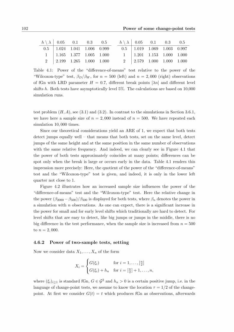
102 Power of some change-point tests
h \ λ 0.05 0.1 0.3 0.5
0.5 1.024 1.041 1.006 0.999
1 1.165 1.377 1.005 1.000
2 2.199 1.265 1.000 1.000
h \ λ 0.05 0.1 0.3 0.5
0.5 1.019 1.069 1.003 0.997
1 1.201 1.153 1.000 1.000
2 2.579 1.000 1.000 1.000
Table 4.1: Power of the “difference-of-means” test relative to the power of the
“Wilcoxon-type” test, βD/βW , for n = 500 (left) and n = 2, 000 (right) observations
of fGn with LRD parameter H = 0.7, different break points [λn] and different level
shifts h. Both tests have asymptotically level 5%. The calculations are based on 10,000
simulation runs.
test problem (H,A), see (3.1) and (3.2). In contrast to the simulations in Section 3.6.1,
we have here a sample size of n = 2, 000 instead of n = 500. We have repeated each
simulation 10, 000 times.
Since our theoretical considerations yield an ARE of 1, we expect that both tests
detect jumps equally well – that means that both tests, set on the same level, detect
jumps of the same height and at the same position in the same number of observations
with the same relative frequency. And indeed, we can clearly see in Figure 4.1 that
the power of both tests approximately coincides at many points; differences can be
spot only when the break is large or occurs early in the data. Table 4.1 renders this
impression more precisely: Here, the quotient of the power of the “difference-of-means”
test and the “Wilcoxon-type” test is given, and indeed, it is only in the lower left
quarter not close to 1.
Figure 4.2 illustrates how an increased sample size influences the power of the
“difference-of-means” test and the “Wilcoxon-type” test. Here the relative change in
the power (β2000−β500)/β500 is displayed for both tests, where βn denotes the power in
a simulation with n observations. As one can expect, there is a significant increase in
the power for small and for early level shifts which traditionally are hard to detect. For
level shifts that are easy to detect, like big jumps or jumps in the middle, there is no
big difference in the test performance, when the sample size is increased from n = 500
to n = 2, 000.
4.6.2 Power of two-sample tests, setting
Now we consider data X1, . . . , Xn of the form
Xi =
G(ξi) for i = 1, . . . , [n2 ]
G(ξi) + hn for i = [n2 ] + 1, . . . , n,
where (ξi)i≥1 is standard fGn, G ∈ G2 and hn > 0 is a certain positive jump, i.e. in the
language of change-point tests, we assume to know the location τ = 1/2 of the change-
point. At first we consider G(t) = t which produces fGn as observations, afterwards

4.6 Simulations 103
0.0 0.1 0.2 0.3 0.4 0.5
0.0
0.2
0.4
0.6
0.8
1.0
Lambda
Power
h=0.5h=1h=2
DiffWilcoxon
Figure 4.1: Power of “difference-of-means” test (blue) and power of “Wilcoxon-type”
test (green) for n = 2, 000 observations of fGn with LRD parameter H = 0.7, different
break points [λn] and different level shifts h. Both tests have asymptotically level 5%.
The calculations are based on 10,000 simulation runs.
0.0 0.1 0.2 0.3 0.4 0.5
0.0
0.5
1.0
1.5
2.0
Lambda
Rel. Increase Power h=0.5
h=1h=2
DiffWilcoxon
Figure 4.2: Relative change of the power of the “difference-of-means” test (blue) and
of the “Wilcoxon-type” test (green) if the sample size increases from n = 500 to n =
2, 000. The simulation is based on fGn with LRD parameter H = 0.7, different break
points [λn], different level shifts h and each 10, 000 simulation runs. Both tests have
asymptotically level 5%.
104 Power of some change-point tests
we look at a transformation G which yields standardised Pareto(3,1) distributed data.
As jump height we choose
hn = cdnn
= cn−D/2
and analyse how well this jump can be detected, both by the two-sample Gauß test
and by the two-sample Wilcoxon test: We test
H : hn = 0 against A1/2,hn : hn > 0.
For the Gauß test, we use the statistic
D1/2,n =1
ndn
[n/2]∑i=1
n∑j=[n/2]+1
(Xj −Xi).
Here we have m = 1, since G is strictly monotone, thus we obtain by Theorem 3.5
D1/2,nD−→ −a1
(Z1(1/2)− 1
2Z1(1)
)D= −a1N (0, σ2
0.5)
with
σ20.5 := Var
[Z1(1/2)− 1
2Z1(1)
]=
1
22H− 1
4, (4.52)
because Z1 is fBm. So the two-sample Gauß test rejects H if
D1/2,n
|a1|σ0.5> zα, (4.53)
where zα denotes the upper α-quantile of the standard normal distribution. By Theo-
rem 4.1, we obtain under the alternative the convergence
D1/2,n
a1σ0.5
D−→ N (0, 1) +c
4a1σ0.5.
For the Wilcoxon test, we compute the statistic
W1/2,n =1
ndn
[n/2]∑i=1
n∑j=[n/2]+1
(IXi≤Xj −
1
2
).
By Theorem 3.4, it holds under the null hypothesis of no change
2√πW1/2,n
σ0.5
D−→ N (0, 1),
with σ0.5 as in (4.52), and the two-sample Wilcoxon test rejects H if
2√πW1/2,n
σ0.5> zα, (4.54)
where zα still denotes the upper α-quantile of the standard normal distribution. In
Theorem 4.2 we have shown that under the alternative
2√πW1/2,n
σ0.5
D−→ N (0, 1) +c 2√π
4σ0.5
∫Rf2(x) dx,
where f denotes the p.d.f. of the observations Xi.
In what follows, we will compare these two tests based on D1/2,n and W1/2,n, as set
in (4.53) and (4.54), in two different data situations.
4.6 Simulations 105
4.6.3 Power of two-sample tests, Gaussian observations
Using the fArma package in R, we have simulated n = 50, 100, 500, 1000, 2000 realiza-
tions ξ1, . . . , ξn of fGn with Hurst parameter H = 0.7 (respectively D = 0.6). At first,
we have considered observations Xi = G(ξi) with G(t) = t, i.e. fGn. To the second
sample of observations, X[n/2]+1, . . . , Xn, we have added a constant, depending on n,
hn = cdnn
= cn−D/2 =
0.102c if n = 2, 000
0.126c if n = 1, 000
0.155c if n = 500
0.251c if n = 100
0.309c if n = 50.
(4.55)
To these data, we have applied the two-sample Gauß test and the 2-sample Wilcoxon
test, as set in (4.53) and (4.54). Here, the first Hermite coefficient of G is a1 = 1 and∫R f
2(x) dx = (2√π)−1 since f is the standard normal p.d.f.. Under 10,000 simulation
runs, we have counted the number of true rejections as an estimate of the power of the
respective test; the results are shown in Table 4.2. In Table 4.3, their quotient is given;
it is close to 1. Our theoretical findings state that
ARE = limn→∞
nDnW
=
(a1
∫R f
2(x) dx∫R J1(x)f(x) dx
)2/D
= 1,
which means that both tests, set on the same level, need on large scale the same number
of observations in order to detect the same jump with a given probability. And indeed,
for the same number of observations and on the same level both tests detect the same
jump nearly equally often. So our theoretical findings that the ARE is 1 for Gaussian
data can already be seen in two sample situations.
Note that the simulations also illustrate that the special form of hn (which is defined
in (4.55) and provided by our limit theorem) is just right: According to our theoretical
findings, a jump(-sequence) of height c hn leads to a non-degenerate limit of the test
statistic. And indeed, for a fixed c, the observed power of each test is nearly the same
for all sample sizes n which is a plausible evidence that the test statistic under data
with jump c hn approaches a certain non-degenerate limit.
4.6.4 Power of two-sample tests, Pareto(3,1) observations
To n realizations ξ1, . . . , ξn of fGn we have now applied the transformation
G(t) =1√3/4
((Φ(t))−1/3 − 3
2
),
which produces observations Xi = G(ξi) which follow a standardised Pareto(3,1) distri-
bution. To the second sample of observations, X[n/2]+1, . . . , Xn, we have again added a
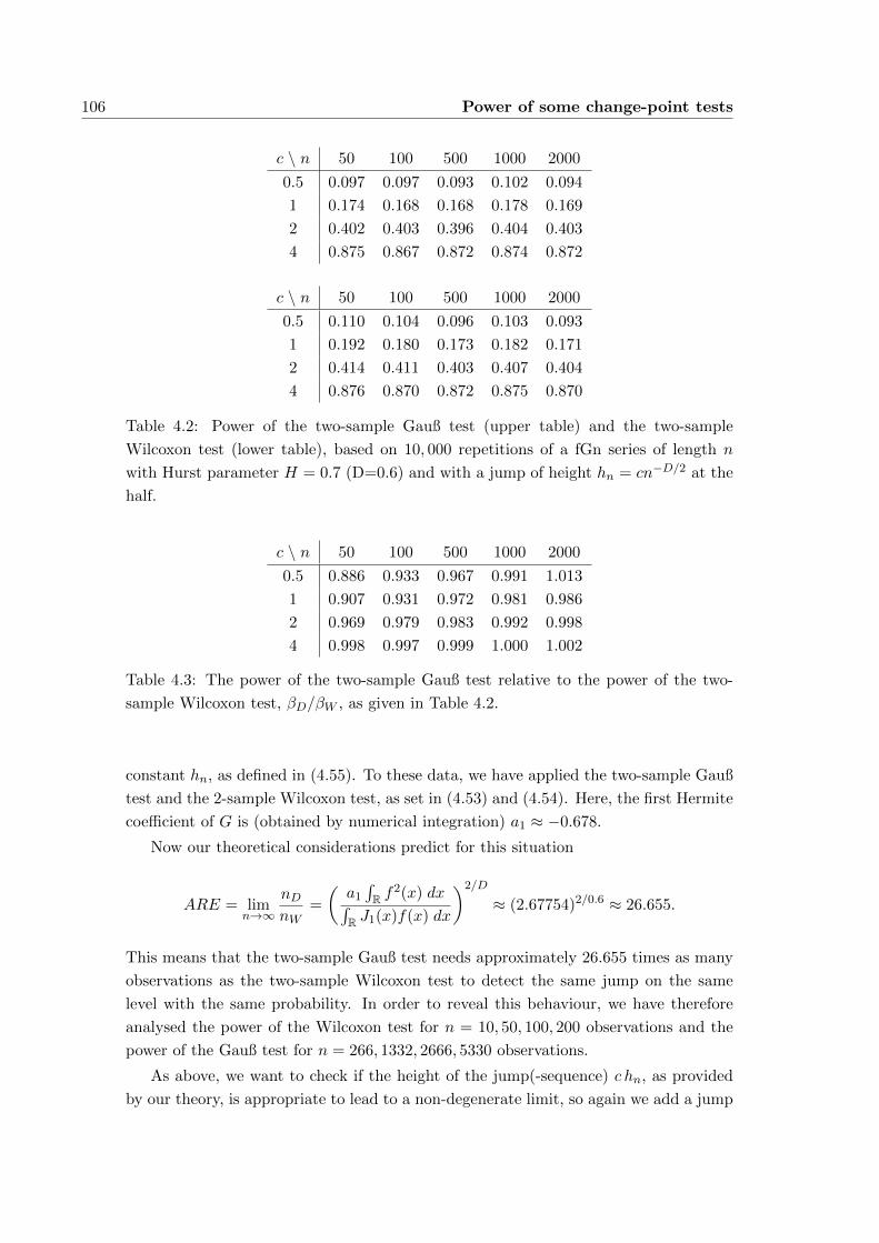
106 Power of some change-point tests
c \ n 50 100 500 1000 2000
0.5 0.097 0.097 0.093 0.102 0.094
1 0.174 0.168 0.168 0.178 0.169
2 0.402 0.403 0.396 0.404 0.403
4 0.875 0.867 0.872 0.874 0.872
c \ n 50 100 500 1000 2000
0.5 0.110 0.104 0.096 0.103 0.093
1 0.192 0.180 0.173 0.182 0.171
2 0.414 0.411 0.403 0.407 0.404
4 0.876 0.870 0.872 0.875 0.870
Table 4.2: Power of the two-sample Gauß test (upper table) and the two-sample
Wilcoxon test (lower table), based on 10, 000 repetitions of a fGn series of length n
with Hurst parameter H = 0.7 (D=0.6) and with a jump of height hn = cn−D/2 at the
half.
c \ n 50 100 500 1000 2000
0.5 0.886 0.933 0.967 0.991 1.013
1 0.907 0.931 0.972 0.981 0.986
2 0.969 0.979 0.983 0.992 0.998
4 0.998 0.997 0.999 1.000 1.002
Table 4.3: The power of the two-sample Gauß test relative to the power of the two-
sample Wilcoxon test, βD/βW , as given in Table 4.2.
constant hn, as defined in (4.55). To these data, we have applied the two-sample Gauß
test and the 2-sample Wilcoxon test, as set in (4.53) and (4.54). Here, the first Hermite
coefficient of G is (obtained by numerical integration) a1 ≈ −0.678.
Now our theoretical considerations predict for this situation
ARE = limn→∞
nDnW
=
(a1
∫R f
2(x) dx∫R J1(x)f(x) dx
)2/D
≈ (2.67754)2/0.6 ≈ 26.655.
This means that the two-sample Gauß test needs approximately 26.655 times as many
observations as the two-sample Wilcoxon test to detect the same jump on the same
level with the same probability. In order to reveal this behaviour, we have therefore
analysed the power of the Wilcoxon test for n = 10, 50, 100, 200 observations and the
power of the Gauß test for n = 266, 1332, 2666, 5330 observations.
As above, we want to check if the height of the jump(-sequence) c hn, as provided
by our theory, is appropriate to lead to a non-degenerate limit, so again we add a jump
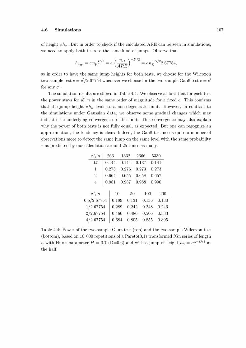
4.6 Simulations 107
of height c hn. But in order to check if the calculated ARE can be seen in simulations,
we need to apply both tests to the same kind of jumps. Observe that
hnW = c n−D/2W = c
( nDARE
)−D/2= c n
−D/2D 2.67754,
so in order to have the same jump heights for both tests, we choose for the Wilcoxon
two-sample test c = c′/2.67754 whenever we choose for the two-sample Gauß test c = c′
for any c′.
The simulation results are shown in Table 4.4. We observe at first that for each test
the power stays for all n in the same order of magnitude for a fixed c. This confirms
that the jump height c hn leads to a non-degenerate limit. However, in contrast to
the simulations under Gaussian data, we observe some gradual changes which may
indicate the underlying convergence to the limit. This convergence may also explain
why the power of both tests is not fully equal, as expected. But one can regognize an
approximation, the tendency is clear: Indeed, the Gauß test needs quite a number of
observations more to detect the same jump on the same level with the same probability
– as predicted by our calculation around 25 times as many.
c \ n 266 1332 2666 5330
0.5 0.144 0.144 0.137 0.141
1 0.273 0.276 0.273 0.273
2 0.664 0.655 0.658 0.657
4 0.981 0.987 0.988 0.990
c \ n 10 50 100 200
0.5/2.67754 0.189 0.131 0.136 0.130
1/2.67754 0.289 0.242 0.248 0.246
2/2.67754 0.466 0.486 0.506 0.533
4/2.67754 0.684 0.805 0.855 0.895
Table 4.4: Power of the two-sample Gauß test (top) and the two-sample Wilcoxon test
(bottom), based on 10, 000 repetitions of a Pareto(3,1) transformed fGn series of length
n with Hurst parameter H = 0.7 (D=0.6) and with a jump of height hn = cn−D/2 at
the half.

108 Power of some change-point tests
Chapter 5
Change-point processes based on
U-statistics
There are several asymptotic results for U -statistics of LRD data (Dehling and Taqqu,
1991; Hsing and Wu, 2004; Beutner and Zahle, 2011; Beutner, Wu and Zahle, 2012,
e.g.). In Chapter 3 we developed a non-parametric change-point test for LRD data
which is based on Wilcoxon’s two-sample test statistic which can be represented as
a U -statistic. We determined its asymptotic distribution under the null hpothesis
that no change occured by representing the test statistic as a functional of the two-
parameter empirical process of the data for which there are limit theorems (Dehling and
Taqqu, 1989, 1991). Since our test is based on the Wilcoxon two-sample rank statistic
Wk,n = (ndn)−1∑k
i=1
∑nj=k+1 IXi≤Xj and since Wk,n in its above representation is a
U -statistic, the natural question arises if the technique can universally be extended to
U -statistics
Uk,n =k∑i=1
n∑j=k+1
h(Xi, Xj)
with a general kernel h. Of course, such a generalization will require more technical
and formal work because a general kernel does not possess the conducive form of the
kernel h(x, y) = Ix≤y, which leads to the Wilcoxon statistic and has substantial formal
similarity to the empirical distribution function. The idea of the proof shall nevertheless
still be to express the statistic as a functional of the empirical process for which we
have an asymptotic theory: As shown in Chapter 3, by the Dudley-Wichura version
of Skorohod’s representation theorem (Shorack and Wellner, 1986, Th. 2.3.4) it follows
from the empirical process non-central limit theorem of Dehling and Taqqu (1989) that
supλ,x
∣∣d−1n [nλ](F[λn](x)− F (x))− J(x)Z(λ)
∣∣ −→ 0 a.s. (5.1)
and
supλ,x
∣∣d−1n (n− [nλ])(F[nλ]+1,n(x)− F (x))− J(x)(Z(1)− Z(λ))
∣∣ −→ 0 a.s., (5.2)
110 Change-point processes based on U-statistics
where Z denotes a certain Hermite process. In this chapter, I will present generaliza-
tions to the work by Dehling, Rooch and Taqqu (2012) and develop limit theorems for
the general U -statistic Uk,n under the null hypothesis of no change in the mean. In
Chapter 6, we present a different approach to the limit behaviour of Uk,n.
5.1 Special kernels
We start with general kernels of a special form: Factorizable kernels h(x, y) = a(x)b(y)
and additive kernels h(x, y) = a(x)+b(y). Note that both types allow a direct approach,
see the remark on page 114. Nevertheless, for illustration of our method, we choose a
technique based on a representation via the e.d.f..
Theorem 5.1 (NCLT for two-sample U -statistics with factorizable kernels). Suppose
that (ξi)i≥1 is a stationary Gaussian process with mean zero, variance 1 and auto-
covariance function as in (1.1) with 0 < D < 1m . Moreover let G : R → R be a
measurable function with E[G(ξi)] = 0 and define
Xk = G(ξk).
Assume that Xk has a continuous distribution function F . Let m denote the Hermite
rank of the class of functions IG(ξi)≤x−F (x), x ∈ R. Assume that h(x, y) = a(x)b(y)
satisfies the following conditions:
(i)∫|a(x)| dF (x) <∞ and
∫|b(x)| dF (x) <∞
(ii) a(x) and b(y) have both bounded total variation.
(iii)∫J(x) da(x) and
∫J(x) db(x) exist and are finite.
Then with the notation of Chapter 3,
1
ndn
[λn]∑i=1
n∑j=[λn]+1
(h(Xi, Xj)−
∫∫h(x1, x2) dF (x1)dF (x2)
), 0 ≤ λ ≤ 1, (5.3)
converges in distribution towards the process
− (1− λ)Z(λ)
∫J(x) da(x)
∫b(x) dF (x)
− λ(Z(1)− Z(λ))
∫J(x) db(x)
∫a(x) dF (x), 0 ≤ λ ≤ 1.
(5.4)
We set Z(λ) = Zm(λ)/m!, where Zm(λ) denotes the m-th order Hermite process.
Remark. (a) Using the special form of the kernel, the statistic (5.3) can be written as
1
ndn
[λn]∑i=1
n∑j=[λn]+1
(a(Xi)b(Xj)− E[a(X)]E[b(X)]) , 0 ≤ λ ≤ 1,
5.1 Special kernels 111
where X ∼ F has the same distribution as the single Xi’s.
(b) Condition (i) is equivalent to E|h(X,Y )| <∞ for independent X,Y ∼ F .
(c) If h has bounded variation in the sense of Hardy-Krause (see Appendix B.3),
then condition (ii) is fulfilled.
Proof. In order to use (5.1) and (5.2), we write sums as integrals with respect to the
e.d.f. Fn and then enforce expressions of type “Fn − F” in our test statistic.
[λn]∑i=1
n∑j=[λn]+1
(h(Xi, Xj)−
∫∫h(x1, x2) dF (x1)dF (x2)
)
= (n− [nλ])
[λn]∑i=1
∫h(Xi, x2) dF[λn]+1,n(x2)− [λn](n− [λn])
∫∫h(x1, x2) dF (x1)dF (x2)
= [λn](n− [nλ])
∫ (∫h(x1, x2) dF[λn]+1,n(x2)
)dF[λn](x1)
−∫∫
h(x1, x2) dF (x1)dF (x2)
= [λn](n− [nλ])
∫ (∫h(x1, x2) d(F[λn]+1,n − F )(x2)
)dF[λn](x1)
+
∫ (∫h(x1, x2) dF (x2)
)d(F[λn] − F )(x1)
(5.5)
and with h(x, y) = a(x)b(y)
= [λn](n− [nλ])
∫a(x) dF[λn](x)
∫b(x) d(F[λn]+1,n − F )(x2)
+
∫a(x) d(F[λn] − F )(x)
∫b(x) dF (x)
= [λn](n− [nλ])
(∫a(x) d(F[λn] − F )(x) +
∫a(x) dF (x)
)∫b(x) d(F[λn]+1,n − F )(x)
+
∫a(x) d(F[λn] − F )(x)
∫b(x) dF (x)
Now we integrate by parts in order to have the “Fn − F” terms as integrands and
the deterministic terms as integrators.∫a(x) d(F[λn] − F )(x) =
[a(x)(F[λn] − F )(x)
]∞−∞ −
∫(F[λn] − F )(x) da(x)∫
b(x) d(F[λn]+1,n − F )(x) =[b(x)(F[λn]+1,n − F )(x)
]∞−∞ −
∫(F[λn]+1,n − F )(x) db(x)
112 Change-point processes based on U-statistics
We assumed by (ii) that a(x) and b(x) have bounded total variation. This ensures that
the integrals on the right-hand side exist, moreover it follows that a(x) and b(x) are
bounded and the boundary terms on the right-hand side vanish. So we obtain
1
ndn
[λn]∑i=1
n∑j=[λn]+1
(h(Xi, Xj)−
∫∫h(x1, x2) dF (x1)dF (x2)
)
=[λn](n− [nλ])
ndn
(∫(F[λn] − F )(x) da(x)−
∫a(x) dF (x)
)∫(F[λn]+1,n − F )(x) db(x)
−∫
(F[λn] − F )(x) da(x)
∫b(x) dF (x)
. (5.6)
We will now show that this converges to the process given in (5.4). We look into the
single terms.
[λn](n− [nλ])
ndn
∫(F[λn]+1,n − F )(x) db(x)− λ
∫J(x)(Z(1)− Z(λ)) db(x)
=[λn]
n
∫d−1n (n− [nλ])
((F[λn]+1,n − F )(x)− J(x)(Z(1)− Z(λ))
)db(x)
+
([λn]
n− λ)∫
J(x)(Z(1)− Z(λ)) db(x)
The first term on the right-hand side converges to 0 due to the bounded total vartiation
of b(x) and (5.2). The second term converges to 0 because we assumed in (iii) that the
integral is finite, and [λn]/n→ λ uniformly. Since ‖F[λn] − F‖∞ → 0 almost surely,∫(F[λn] − F )(x) da(x) −→ 0.
Finally
− [λn](n− [nλ])
ndn
∫(F[λn] − F )(x) da(x) + (1− λ)
∫J(x)Z(λ) da(x)
= −n− [λn]
n
∫ (d−1n [λn](F[λn] − F )(x)− J(x)Z(λ)
)da(x)
−(n− [λn]
n− (1− λ)
)∫J(x)Z(λ) da(x)
converges to 0 by the same arguments as above: a(x) is of bounded variation and
because of (5.1), the first integral on the right-hand side vanishes; the second integral
is finite by assumtion (iii), and (n−[λn])/n→ (1−λ) uniformly. For putting everything
together in (5.6), note that∫J(x) da(x) and
∫J(x) db(x) are finite due to condition (iii).
For additive kernels, we obtain a quite similar result.
Theorem 5.2 (NCLT for two-sample U -statistics with additive kernels). Suppose that
(ξi)i≥1 is a stationary Gaussian process with mean zero, variance 1 and auto-covariance
5.1 Special kernels 113
function as in (1.1) with 0 < D < 1m . Moreover let G : R→ R be a measurable function
with E[G(ξi)] = 0 and define
Xk = G(ξk).
Assume that Xk has a continuous distribution function F . Let m denote the Hermite
rank of the class of functions IG(ξi)≤x−F (x), x ∈ R. Assume that h(x, y) = a(x)+b(y)
satisfies the following conditions:
(i)∫|a(x)| dF (x) <∞ and
∫|b(x)| dF (x) <∞
(ii) a(x) and b(y) have both bounded total variation.
(iii)∫J(x) da(x) and
∫J(x) db(x) exist and are finite.
Then with the notation of Chapter 3,
1
ndn
[λn]∑i=1
n∑j=[λn]+1
(h(Xi, Xj)−
∫∫h(x1, x2) dF (x1)dF (x2)
), 0 ≤ λ ≤ 1,
converges in distribution towards the process
−(1− λ)Z(λ)
∫J(x) da(x)− λ(Z(1)− Z(λ))
∫J(x) db(x), 0 ≤ λ ≤ 1. (5.7)
Again, we set Z(λ) = Zm(λ)/m!, where Zm(λ) denotes the m-th order Hermite process.
Remark. (a) Due to the special form of the kernel, the statistic can also be written as
1
ndn
[λn]∑i=1
n∑j=[λn]+1
((a(Xi)− E[a(X)]) + (b(Xj)− E[b(X)])) , 0 ≤ λ ≤ 1,
or
n− [λn]
ndn
[λn]∑i=1
(a(Xi)− E[a(X)]) +[λn]
ndn
n∑j=[λn]+1
(b(Xj)− E[b(X)]) , 0 ≤ λ ≤ 1,
where X ∼ F has the same distribution as the single Xi’s.
(b) The conditions under which Theorem 5.2 holds are the same as for Theorem 5.1.
Proof. The idea behind the proof stays the same: We aim to express the statistic as
a functional of the empirical process such that we can use the convergence theorems
114 Change-point processes based on U-statistics
(5.1) and (5.2). We start as in the proof before, and from (5.5) we obtain, using that
h(x, y) = a(x) + b(y),
[λn]∑i=1
n∑j=[λn]+1
(h(Xi, Xj)−
∫∫h(x1, x2) dF (x1)dF (x2)
)
= [λn](n− [nλ])
∫ (∫a(x1) d(F[λn]+1,n − F )(x2)
)dF[λn](x1)
+
∫ (∫a(x1) dF (x2)
)d(F[λn] − F )(x1)
+
∫ (∫b(x2) d(F[λn]+1,n − F )(x2)
)dF[λn](x1)
+
∫ (∫b(x2) dF (x2)
)d(F[λn] − F )(x1)
= [λn](n− [nλ])
∫a(x) d(F[λn] − F )(x) +
∫b(x) d(F[λn]+1,n − F )(x)
,
where we have used that F and Fn are distribution functions and that for any pair
of c.d.f.’s F , G it holds∫dF = 1 and
∫d(F − G) = 0. Here it also contributes
condition (i). Observe that by integration by parts∣∣∣∣∫ a(x) dF[λn](x)
∣∣∣∣ =
∣∣∣∣∫ a(x) d(F[λn] − F )(x) +
∫a(x) dF (x)
∣∣∣∣≤∣∣∣∣∫ (F[λn] − F )(x) da(x)
∣∣∣∣+
∣∣∣∣∫ a(x) dF (x)
∣∣∣∣ <∞.Now we integrate by parts in order to have the “Fn − F” terms as integrands and the
deterministic terms as integrators, exactly as in the proof before. This yields
1
ndn
[λn]∑i=1
n∑j=[λn]+1
(h(Xi, Xj)−
∫∫h(x1, x2) dF (x1)dF (x2)
)
= [λn](n− [nλ])
−∫
(F[λn] − F )(x) da(x)−∫
(F[λn]+1,n − F )(x) db(x)
. (5.8)
As in the proof before, due to the bounded total vartiation of a(x), b(x) and in virtue
of (5.1) and (5.2), this converges to the process given in (5.7).
Remark. The just treated cases of special kernels, h(x, y) = a(x)b(y) and h(x, y) =
a(x)+b(y), allow both a direct approach: one can trace them back to the limit theorems
for single partial sums, as presented in Theorem (1.1). For example for factorizable
kernels one has
1
dn(ma)dn(mb)
[λn]∑i=1
n∑j=[λn]+1
a(Xi)b(Xj) =
1
dn(ma)
[λn]∑i=1
a(Xi)
1
dn(mb)
n∑j=[λn]+1
b(Xj)
,

5.2 General kernels 115
where ma, mb are the Hermite rank of the functions a(G(·)), b(G(·)) respectively. For
such an approach, one needs the joint convergence. Compare this to the approach in
Chapter 6.
5.2 General kernels
Theorem 5.3 (General NCLT for two-sample U -statistics). Suppose that (ξi)i≥1 is a
stationary Gaussian process with mean zero, variance 1 and auto-covariance function
as in (1.1) with 0 < D < 1m . Moreover let G : R → R be a measurable function with
E[G(ξi)] = 0 and define
Xk = G(ξk).
Assume that Xk has a continuous distribution function F . Let m denote the Hermite
rank of the class of functions IG(ξi)≤x − F (x), x ∈ R. Define
h(x1) :=
∫h(x1, x2) dF (x2)
and assume that the following conditions hold:
(i) The kernel h(x, y) is of bounded total variation in each variable (each with the
other one fixed).
(ii) h(x, y) satisfies the following growth conditions:
supx∈R
limy→∞
(h(x, y)(1− F (y))− h(x,−y)F (−y)
)= 0
limx→∞
(h(x)(1− F (x))− h(−x)F (−x)
)= 0
(iii) h(x1) is of bounded total variation.
(iv)∫d|h(x1, x2)(x2)|TV ≤ c <∞
(v)∫J(x1) dh(x1) and
∫ (∫J(x2) dh(x1, x2)(x2)
)dF (x1) exist and are finite.
Then, with the notation of Chapter 3,
1
ndn
[λn]∑i=1
n∑j=[λn]+1
(h(Xi, Xj)−
∫∫h(x1, x2) dF (x1)dF (x2)
), 0 ≤ λ ≤ 1,
converges in distribution towards the process
− (1− λ)Z(λ)
∫J(x1) dh(x1)
− λ(Z(1)− Z(λ))
∫ (∫J(x2) dh(x1, x2)(x2)
)dF (x1), 0 ≤ λ ≤ 1.
(5.9)
Again, we set Z(λ) = Zm(λ)/m!, where Zm(λ) denotes the m-th order Hermite process.
116 Change-point processes based on U-statistics
Remark. (a) Conditions (i)–(iv) are sufficient, but not neccessary. During the proof,
we will have to ensure that certain integrals are finite; the conditions guarantee upper
bounds. Of course in particular cases, the conditions may be violated, but neverthe-
less the respective integrals may be finite. This is also the case for condition (ii) of
Theorem 5.1 and Theorem 5.2: It may be too restrictive.
(b) Let us spend a moment to discuss the conditions and some possible implications:
• Condition (i) means that the kernel function does not fluctuate too much. It
ensures that one can one-dimensionally integrate with h as integrator (with one
variable fixed). The condition is met for any bounded function which is monotone
in each variable, like h(x, y) = Ix≤y (which, by the way, is not of bounded total
variation, see Section B.3.2), while it is not met for any unbounded function like
h(x, y) = xy.
• Condition (ii) is also needed for the integration by parts: If the tails of the kernel
h grow to fast, the boundary terms may not vanish. If h is bounded, (ii) is always
fulfilled.
• Condition (iii) is a sufficient condition that∫f(x)dh(x) is finite for bounded f .
If h is factorizable, (i) implies (iii).
• Condition (iv) demands that h(x1, x2) is bounded in x1 (which is also required
by condition (i)). If h(x1, x2) is monotone increasing in x2, (iv) reduces to∣∣∫ dh(x1, x2)(x2)∣∣ ≤ c <∞.
• If J is bounded, (iii) and (iv) imply (v). By the remark following the proof,
one can express∫J(x1) dh(x1) as a Hermite coefficient of the function h(G(·)).
Thus if h(G(·)) =∫h(G(·), y) dF (y) ∈ L2(R,N ), then
∫J(x1) dh(x1) exists and
is finite.
Proof. As before, we express the statistic as a functional of the empirical process. For
this purpose, we write sums as integrals with respect to the e.d.f. Fn and enforce
expressions of type “Fn − F”. By (5.5) it is
[λn]∑i=1
n∑j=[λn]+1
(h(Xi, Xj)−
∫∫h(x1, x2) dF (x1)dF (x2)
)
= [λn](n− [nλ])
∫ (∫h(x1, x2) d(F[λn]+1,n − F )(x2)
)dF[λn](x1)
+
∫ (∫h(x1, x2) dF (x2)
)d(F[λn] − F )(x1)
,

5.2 General kernels 117
and now we integrate by parts in order to get the “Fn − F” terms as integrands and
the deterministic terms as integrators.
∫h(x1, x2) d(F[λn]+1,n − F )(x2)
=[h(x1, x2) · (F[λn]+1,n − F )(x2)
]∞x2=−∞ −
∫(F[λn]+1,n − F )(x2) dh(x1, x2)(x2)
(5.10)∫ (∫h(x1, x2) dF (x2)
)d(F[λn] − F )(x1)
=[h(x1) · (F[λn] − F )(x1)
]∞x1=−∞
−∫
(F[λn] − F )(x1) dh(x1) (5.11)
The boundary terms vanish due to assumption (ii) and the remaining integrals are
defined because of assumptions (i) and (iii). It is important that the boundary term
in (5.10) does not only vanish for any fixed x1, but uniformly, due to assumption (ii),
because the integration by parts takes place in an integrand of an integral with respect
to F[λn](x1). (Another approach is possible to handle the term on the right-hand side of
(5.11); see the remark following this proof.) After integration by parts we thus obtain
1
ndn
[λn]∑i=1
n∑j=[λn]+1
(h(Xi, Xj)−
∫∫h(x1, x2) dF (x1)dF (x2)
)
=[λn](n− [nλ])
ndn
∫ (−∫
(F[λn]+1,n − F )(x2) dh(x1, x2)(x2)
)dF[λn](x1)
−∫
(F[λn] − F )(x1) dh(x1)
. (5.12)
We now go into both terms and show that they converge to the limit given in (5.9).
[λn](n− [nλ])
ndn
∫(F[λn] − F )(x1) dh(x1)− (1− λ)
∫J(x1)Z(λ) dh(x1)
=n− [nλ]
n
∫ (d−1n [λn](F[λn] − F )(x1)− J(x1)Z(λ)
)dh(x1)
+
(n− [λn]
n− (1− λ)
)∫J(x1)Z(λ) dh(x1) (5.13)
The first summand on the right-hand side converges to zero because of (5.1) and
the bounded total variation of h due to condition (iii), the second summand since
sup0≤λ≤1 |(n − [nλ])/n − (1 − λ)| → 0 as above and since∫J(x1) dh(x1) < ∞ by
assumption (v).
118 Change-point processes based on U-statistics
[λn](n− [nλ])
ndn
∫ (∫(F[λn]+1,n − F )(x2) dh(x1, x2)(x2)
)dF[λn](x1)
− λ∫ (∫
J(x2)(Z(1)− Z(λ)) dh(x1, x2)(x2)
)dF (x1)
=[nλ]
n
∫ ∫d−1n (n− [nλ])(F[nλ]+1,n − F )(x2)
− J(x2)(Z(1)− Z(λ)) dh(x1, x2)(x2)
dF[nλ](x1)
+[nλ]
n(Z(1)− Z(λ))
∫ (∫J(x2) dh(x1, x2)(x2)
)d(F[nλ] − F )(x1)
+
([nλ]
n− λ)
(Z(1)− Z(λ))
∫ (∫J(x2) dh(x1, x2)(x2)
)dF (x1) (5.14)
All three terms on the right-hand side converge to zero. For the last term this is
a consequence of sup0≤λ≤1 |[nλ]/n − λ| → 0 as above and of assumption (v). The
convergence of the first term follows from (5.2) and from assumption (iv): With the
abbreviation Kn,λ(x) := d−1n (n − [nλ])(F[nλ]+1,n(x) − F (x)) − J(x)(Z(1) − Z(λ)), the
first term on the right-hand side of (5.14) is∫∫Kn,λ(x2) dh(x1, x2)(x2) dF[nλ](x1)
≤ supλ,x|Kn,λ(x)|
∫∫d|h(x1, x2)(x2)|TV dF[nλ](x1)
≤ supλ,x|Kn,λ(x)| c‖F[λn]‖TV ,
due to assumption (iv). This goes to 0 because supλ,x |Kn,λ(x)| → 0 a.s. by (5.2).
The second term in (5.14) can be written as
[nλ]
n
∫ (∫J(x2) dh(x1, x2)(x2)
)d(F[nλ] − F )(x1)
=1
n
[λn]∑i=1
∫J(x2) dh(Xi, x2)(x2)− E
[∫J(x2) dh(X1, x2)(x2)
].
The ergodic theorem states that k−1∑k
i=1(f(Xi) − Ef(Xi)) → 0 a.s., and thus can
be applied here with f(x) =∫J(t) dh(x, t)(t); the neccessary requirement E|f(Xi)| =∫
|f(x)|dF (x) <∞ is guaranteed by assumption (v).
So (5.13) and (5.14) converge to zero, and bearing this in mind, (5.12) proves the
statement.
5.2 General kernels 119
Remark. The preceding proof started with writing
[λn]∑i=1
n∑j=[λn]+1
(h(Xi, Xj)−
∫∫h(x1, x2) dF (x1)dF (x2)
)
= [λn](n− [nλ])
∫ (∫h(x1, x2) d(F[λn]+1,n − F )(x2)
)dF[λn](x1)
+
∫ (∫h(x1, x2) dF (x2)
)d(F[λn] − F )(x1)
. (5.15)
Using integration by parts, we showed that the second term on the right-hand side of
(5.15) converges to
−(1− λ)
∫J1(x1)Z(λ)dh(x1),
where Z(λ) = Zm(λ)/m! and m is the Hermite rank of the class of functions IG(ξ)≤x−F (x). Note that another approach is possible since the second term on the right-hand
side of (5.15) can be written as
[λn](n− [nλ])
ndn
1
[λn]
[λn]∑i=1
(h(Xi)− Eh(Xi)
)D−→ (1− λ)
app!Zp(λ)
by direct application of Theorem 1.1, where p denotes the Hermite rank of h(G(·)) and
ap is the associated Hermite coefficient.
This means that
−(1− λ)
∫J1(x1)Z(λ)dh(x1)
D= (1− λ)
app!Zp(λ) (5.16)
and as a consequence, it follows that first both Hermite ranks are the same, m = p. In
other words, m is the smallest non-zero integer which satisfies
E[h(G(ξ))Hm(ξ)
]6= 0
E[(IG(ξ)≤x − F (x))Hm(ξ)
]6= 0 for some x ∈ R
(and it satisfies both conditions if it satisfies one of them). Second, relation (5.16) may
help to evaluate the constants on either side. As an example, we consider the case
G(t) = t (which entails m = 1 and Hm(x) = x). On the left hand side, we obtain
−∫J1(x) dh(x) = −
∫∫Is≤xs dΦ(s) dh(x)
=
∫ϕ(x) dh(x) since
∫Is≤xs dΦ(s) = −ϕ(x)
= −∫h(x) dϕ(x) by integration by parts
= −∫∫
h(x, y) dΦ(y) dϕ(x) by definition of h
=
∫∫h(x, y)x dΦ(x) dΦ(y) with
dϕ(x)
dx= −xϕ(x).
120 Change-point processes based on U-statistics
For the expression on the right-hand side of (5.16), we obtain in our example
a1 = E[h(ξ)Hm(ξ)
]=
∫h(x)x dΦ(x)
=
∫∫h(x, y)x dΦ(x) dΦ(y),
which is obviously the same.
5.3 Examples
The kernel h(x, y) = Ix≤y
In Chapter 3, we have shown that the technique of Theorem 5.3 works for the kernel
h(x, y) = Ix≤y which yields the Mann-Whitney-Wilcoxon statistic
W[λn],n =1
ndn
[λn]∑i=1
n∑j=[λn]+1
(IXi≤Xj −
1
2
),
but of course we can get the same result as well from the general approach.
General case
We consider data of the general type Xi = G(ξi) and check the consitions of Theo-
rem 5.3:
(i) Observe that h(x, y) = Ix≤y = H(y − x), where H denotes the Heaviside step
function. So for a fixed x or a fixed y, the kernel h(x, y) = H(y−x) is of bounded
variation (it has each only one jump of height 1).
(ii) h is bounded, so the growth conditions are fulfilled.
(iii) We have
h(x1) =
∫h(x1, x2) dF (x2) =
∫ ∞x1
dF (x2) = 1− F (x1),
and this is of bounded total variation since F is monotone and bounded.
(iv) The kernel h can be represented as a Heaviside step function H, see above, and
H is the integral of the Dirac delta function. Thus we have
dh(x1, x2)(x2) = d(Ix1≤x2)(x2) = δx1(x2)dx2,
where δa(x) is the Dirac delta function with mass in point a. We obtain∣∣∣∣∫Rdh(x1, x2)(x2)
∣∣∣∣ =
∣∣∣∣∫Rδx1(x2)dx2
∣∣∣∣ = 1 <∞.
5.3 Examples 121
(v) By the above calculations it holds∫J(x1) dh(x1) = −
∫J(x1) dF (x1)
and ∫∫J(x2) dh(x1, x2)(x2) dF (x1) =
∫J(x1) dF (x1).
|∫J(x) dF (x)| is finite, because with J(x) = Jm(x) = E
[Hm(ξ)IG(ξ)≤x
]it
equals ∣∣∣∣∫∫R2
Hm(s)IG(s)≤x dΦ(s) dF (x)
∣∣∣∣ ≤ ∫∫R2
|Hm(s)| dΦ(s) dF (x),
and Hm is a polynomial and thus integrable with respect to the standard normal
density, moreover F is a c.d.f..
So Theorem 5.3 reproduces the result of Chapter 3: W[λn],n converges in distribution
to the process
(Z(λ)− λZ(1))
∫J(x) dF (x).
In fact, we have just shown a little (but essential) bit more, namely that the integrals
in the limit are always finite such that the limit process is not ∞.
Gaussian observations
Let us also consider the Gaussian case, i.e. the special case G(t) = t such that the
process (Xi)i≥1 = (ξi)1≥1 is standard normally distributed with auto-covariance func-
tion γ(k) = k−DL(k). F is then the c.d.f. of a Gaussian variable, denoted by Φ. We
consider the expansion
IX≤x − F (x) =∞∑q=m
Jq(x)
q!Hq(X)
with Jq(x) = E[IX≤xHq(X)
]. The Hermite rank is m = 1, because
Jm(x) = E[Hm(ξ)IG(ξ)≤x
]= E
[ξIξ≤x
]= −ϕ(x),
is the negative of the p.d.f. of a Gaussian variable and non-zero. Above we have verified
almost all conditions of Theorem 5.3, we only need to check that the limit is finite, but
this is the case because∫R ϕ(x) dΦ(x) = (2
√π)−1 <∞, so Theorem 5.3 can be applied.
It states that W[λn],n converges in distribution to(− 1
2√π
)(Z(λ)− λZ(1)),
where Z(λ) = B1−D/2(λ) denotes the standard fBm with parameter H = 1−D/2.
122 Change-point processes based on U-statistics
If we fix λ, we obtain a result on the two-sample Wilcoxon test under LRD data:
UW,[λn],n =n−2+D/2L(n)−1/2
σW
[λn]∑i=1
n∑j=[λn]+1
(IXi≤Xj −
1
2
)D−→ N (0, 1)
with
σ2W :=
c1
4πVar[Z(λ)−λZ(1)] =
2
4π(1−D)(2−D)
(λ2 − λ+ (1− λ)λ2−D + λ(1− λ)2−D) .
The kernel h(x, y) = x− y
This kernel leads to the difference of means statistic
1
ndnUdiff,[λn],n = D[λn],n =
1
ndn
[λn]∑i=1
n∑j=[λn]+1
(Xi −Xj)
=[λn](n− [λn])
ndn
(X[λn] − X[λn]+1,n
),
where X[λn] denotes the arithmetic mean of the first [λn] observations and X[λn]+1,n
denotes the arithmetic mean of the last n− [λn] observations. Here, the conditions of
Theorem 5.3 are not met; nevertheless, if we ignore this incommodious fact for reasons
of inquisitiveness, carfreely applying the theorem yields the correct limit behaviour. In
order to handle the conditions that involve F , we consider the Gaussian case: G(t) = t
such that m = 1, J(x) = −ϕ(x), F (x) = Φ(x).
(i) The kernel h(x, y) = x − y is not bounded in both variables, thus it does not
have bounded total variation in its single variables. Nevertheless, it has locally
bounded total variation since it is continuous.
(ii) We have
h(x1) =
∫Rh(x1, x2) dF (x2) =
∫R
(x1 − x2) dΦ(x2) = x1.
Φ(x) converges to its limits, as x→ ±∞, fast enough, so that the growth condi-
tions are fulfilled.
(iii) As the kernel itself, h(x1) = x1 is only of locally bounded variation, not of
bounded total variation at all, since it is unbounded.
(iv) We have
dh(x1, x2)(x2) = d(x1 − x2)(x2) = −dx2,
and of course,∫R dh(x1, x2)(x2) is not bounded. Nevertheless, the integrator has
locally bounded variation again.
5.4 Simulations 123
(v) Both integrals have the same absolute value, namely∣∣∣∣∫RJ(t) dh(x, t)(t)
∣∣∣∣ =
∫Rϕ(t) dt = 1 <∞,
thus the integrals in the limit exist and are finite.
So, if one ignored that some of the conditions are violated, Theorem 5.3 would state
that Udiff,[λn],n converges in distribution to the process
(1− λ)Z(λ)
∫ϕ(x1) dx1 − λ(Z(1)− Z(λ))
∫ (∫ϕ(x2) dx2
)dΦ(x1)
= (1− λ)Z(λ)− λ(Z(1)− Z(λ))
= Z(λ)− λZ(1),
where Z(λ) = B1−D/2(λ) denotes the standard fBm with parameter H = 1 − D/2.
This “result” is confirmed by the calculations from Section 3.4.2 and by Horvath and
Kokoszka (1997).
If we fix the parameter λ and change some notation, we reproduce the results from
the introductory consideration of X − Y . Set Yj := X[λn]+j , and Theorem 5.3 states
1
ndnUdiff,[λn],n = D[λn],n =
[λn](n− [λn])
n dn
(X[λn] − Yn−[λn]
)D−→ Z(λ)− λZ(1).
It follows thatnD/2L(n)−1/2
(X[λn] − Yn−[λn]
)√c1 Var[Z(λ)− λZ(1)]
D−→ N (0, 1),
and since the auto-covariace of fBm is known so that Var[Z(λ)− λZ(1)] can be calcu-
lated, after some algebra we find that
c1 Var[Z(λ)− λZ(1)] =2
(1−D)(2−D)
λ1−D + (1− λ)1−D − 1
λ(1− λ),
which is nothing else than the statement of Theorem 2.3.
5.4 Simulations
I have simulated time series ξ1, . . . , ξn of fGn for different Hurst parameters H (respec-
tively D = 2− 2H). In this model, the auto-covariances are
γk ∼ H(2H − 1)k2H−2 =
(1− D
2
)(1−D)k−D.
For each a set of n observations (for varying sample sizes n) and different cutting points
λ I have calculated the two-sample Wilcoxon test statistic
1
σW n2−D2
UW,[λn],n =1
σW
n−2+D2
[λn]∑i=1
n∑j=[λN ]+1
(Iξi≤ξj −
1
2
)
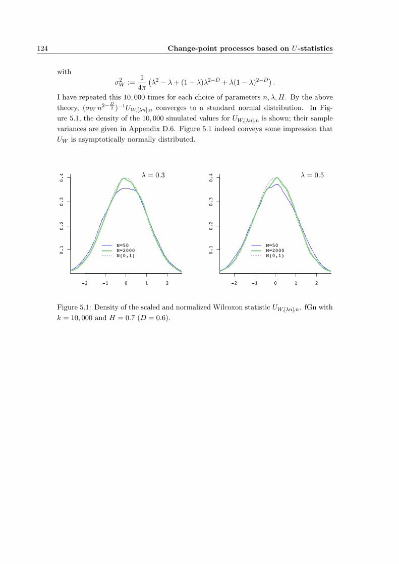
124 Change-point processes based on U-statistics
with
σ2W :=
1
4π
(λ2 − λ+ (1− λ)λ2−D + λ(1− λ)2−D) .
I have repeated this 10, 000 times for each choice of parameters n, λ,H. By the above
theory, (σW n2−D2 )−1UW,[λn],n converges to a standard normal distribution. In Fig-
ure 5.1, the density of the 10, 000 simulated values for UW,[λn],n is shown; their sample
variances are given in Appendix D.6. Figure 5.1 indeed conveys some impression that
UW is asymptotically normally distributed.
-2 -1 0 1 2
0.1
0.2
0.3
0.4
N=50N=2000N(0,1)
-2 -1 0 1 2
0.1
0.2
0.3
0.4
N=50N=2000N(0,1)
λ = 0.3 λ = 0.5
Figure 5.1: Density of the scaled and normalized Wilcoxon statistic UW,[λn],n. fGn with
k = 10, 000 and H = 0.7 (D = 0.6).
Chapter 6
Change-point processes based on
U-statistics, a direct approach
In Chapter 5 we analysed the limit behaviour of the general change-point statistic
k∑i=1
n∑j=k+1
h(Xi, Xj)
with kernel h. In this chapter we make a different approach to this two-sample U -
statistic. As a start, we consider a stationary Gaussian process (ξi)i≥1 with mean
zero, variance 1 and auto-covariance function (1.1) and a function h ∈ L2(R,N ). As
described in Section 1.4.2, in order to analyse the limit behaviour of a partial sums of
observations h(ξ1), . . . , h(ξn), it is useful to expand h in Hermite polynomials. Because
under some assumptions, only the first term in this expansion contributes to the limit,
and one obtains the elegant Theorem 1.1,
1
dn
[λn]∑i=1
h(ξi)D−→ am
m!Zm(λ),
where dn = cmn2−DmLm(n), cm = 2m!((1−Dm)(2−Dm))−1, m denotes the Hermite
rank of h, am the associated Hermite coefficient and where Zm is them-th order Hermite
process. In order to analyse the limit behaviour of two-sample U -statistics
Uλ,n =
[λn]∑i=1
n∑j=[λn]+1
h(ξi, ξj), (6.1)
we will follow a similar route: We will expand h into Hermite polynomials and deduce
the limit behaviour of Uλ,n from this expansion. Due to the dependencies of the (ξi)i≥1,
some problems will arise.
In the one-sample case, each summand of a partial sum∑[λn]
i=1 h(ξi) contains only
one single observation ξi ∼ N (0, 1). Now in order to handle the partial sum, we use
126 Change-point processes based on U-statistics, a direct approach
that Hermite polynomials form an orthogonal basis of L2(R,N ), the space of square-
integrable functions on R with respect to the standard normal measure1 ϕ(x)dx: We
expand h into Hermite polynomials, and this expansion is the same for each summand
in the partial sum∑[λn]
i=1 h(ξi). In the two-sample case, the situation is different: Each
summand in (6.1) contains now a pair of observations (ξi, ξj) ∼ N (0, γ|i−j|) and thus
lives each in another space L2(R2,Nγk), the space of square-integrable functions on R2
with respect to the normal measure ϕk(x, y)dx dy where
ϕk(x, y) =1
2π|Σγk |1/2exp
(−1
2(x, y)TΣ−1
γk(x, y)
)is the p.d.f. of a (two-dimensional)N2(0,Σγk)-distributed random vector with k = |i−j|and
Σγk =
(1 γk
γk 1
).
Thus we would have to expand each summand of Uλ,n into a different set of polynomials,
which is far away from handy, not to mention the question which would be the “Hermite
polynomials” in the space L2(R2,Nγk), i.e. appropriate orthogonal polynomials under
a normal measure with non-trivial covariance matrix – and if the limit theory applies
for them.
Thus we will expand Uλ,n in usual Hermite polynomials as if (ξi, ξj) were indepen-
dent, such that these problems do not arise. Instead, we have to find conditions that
guarantee that this formal expansion converges and really represents Uλ,n.
This approach, which we restricted for a start to Gaussian data ξ1, . . . , ξn, can of
course be extended to general dataG(ξ1), . . . , G(ξn) by considering the kernel h(G(x), G(y))
instead of h(x, y).
6.1 The limit distribution under the null hypothesis
Let (ξi)i≥1 be a stationary Gaussian processes with mean zero, variance 1 and auto-
covariance function (1.1). We assume that we observe n data and that this series is cut
into two pieces at point [λn], λ ∈ (0, 1), so that we have artificially two samples:
ξ1, ξ2, . . . , ξ[λn] and ξ[λn]+1, ξ[λn]+2, . . . , ξn
We now want to study the asymptotic behaviour of the two-sample U -statistic
Uλ,n =
[λn]∑i=1
n∑j=[λn]+1
h(ξi, ξj),
1Sometimes we denote this measure simply by N , i.e. like the normal distribution.
6.1 The limit distribution under the null hypothesis 127
which is based on these observations, with a measurable kernel function h : R2 → R,
h ∈ L2(R2,N ). We can assume without loss of generality that E[h(ξ, η)] = 0 (otherwise
just substract the mean). Then we have the Hermite expansion
h(x, y) =∞∑
k,l=0
aklk! l!
Hkl(x, y) =∞∑
k,l=0
aklk! l!
Hk(x)Hl(y). (6.2)
This is an L2 expansion with respect to the bivariate standard normal density. In this
expansion, the coefficients are
akl = E [h(ξ, η)Hk(ξ)Hl(η)] =
∫∫R2
h(x, y)Hk(x)Hl(y)ϕ(x)ϕ(y) dx dy.
Note that because of the assumption that h is centralised, a0,0 = 0 always. We would
like to order the terms in this expansion (6.2) according to the size of k + l:
h(x, y) =∞∑q=m
∑k,l:
k+l=q
aklk! l!
Hk(x)Hl(y), (6.3)
where m is the smallest integer for which there exists a non-zero Hermite coefficient
akl 6= 0 with k + l = m. m is called the Hermite rank of h(x, y).
Definition 6.1 (Hermite rank for two-dimensional functions). The Hermite rank of a
function h(x, y) is defined as
m = infk + l | k, l ≥ 0, akl 6= 0,
where akl is the coefficient in the Hermite expansion (6.3).
In our setting, a0,0 = 0 always, as stated above, so the kernel h has always Hermite
rank m ≥ 1. In order to show the convergence of Uλ,n with h represented by its Hermite
expansion (6.3), we need a multi-dimensional version of Theorem 1.1. This result can
be obtained using the same techniques that yield the one-dimensional NCLT. Details
for the two-dimensional case will appear in a forthcoming paper by Taqqu (2012).
Theorem 6.1 (Multi-dimensional NCLT for LRD processes). For any 1 ≤ m ≤ 1/D 1
dn(1)
[λ1n]∑i=1
H1(ξi),1
dn(2)
[λ2n]∑i=1
H2(ξi), . . . ,1
dn(m)
[λmn]∑i=1
Hm(ξi)
converges in distribution to the m-dimensional process(
Z1(λ1)
1!,Z2(λ2)
2!, . . . ,
Zm(λm)
m!
)in D[0, 1]m, where
d2n(k) = ckn
2−DkLk(n)
is the usual scaling for the partial sum of the k-th Hermite polynomial and Zk denotes
the k-th order Hermite process, as defined in (1.11).

128 Change-point processes based on U-statistics, a direct approach
Definition 6.2 (Centralized/normalized Lp(R2)-functions). Let ξ, η ∼ N (0, 1) be two
independent standard normal random variables. We define
G1(R2,N ) := G : R2 → R integrable | E[G(ξ, η)] = 0 ⊂ L1(R2,N ),
the class of (with respect to the standard normal measure) centralized and integrable
functions on R2, and
G2(R2,N ) := G : R2 → R measurable | E[G(ξ, η)] = 0, E[G2(ξ, η)] = 1 ⊂ L2(R2,N ),
the class of (with respect to the standard normal measure) normalized and square-
integrable functions on R2.
Any function G : R2 → R which is measurable with mean zero and finite variance
under standard normal measure can be normalized by dividing the standard deviation,
so it can be considered as a function in G2 = G2(R2,N ).
Theorem 6.2. Let (ξi)i≥1 be a stationary Gaussian process with mean 0, variance 1
and covariances (1.1). Let Dm < 1 and let h ∈ G2(R2,N ) be a function with Hermite
rank m whose Hermite coefficients satisfy∑k,l
|akl|√k! l!
<∞. (6.4)
Then as n→∞
1
d′n n
∣∣∣∣∣∣∣∣[λn]∑i=1
n∑j=[λn]+1
h(ξi, ξj)−∑k,l:
k+l=m
aklk! l!
[λn]∑i=1
n∑j=[λn]+1
Hk(ξi)Hl(ξj)
∣∣∣∣∣∣∣∣L1
−→ 0
uniformly in λ ∈ [0, 1] and
1
d′n n
[λn]∑i=1
n∑j=[λn]+1
h(ξi, ξj)D−→
∑k,l:
k+l=m
akl(k! l!)2
(ckcl)1/2Zk(λ)(Zl(1)− Zl(λ)) (6.5)
in D[0, 1], λ ∈ [0, 1], where
d′2n = n2−mDL(n)m (6.6)
and the Zk(λ), k = 0, . . . ,m, are dependent processes which can be expressed as k-fold
Wiener-Ito-Integrals, see (1.11).
Remark. (a) The scaling factor (6.6) differs slightly from the usual scaling (1.12): It
does not include the normalizing constant cm. This is caused by the fact that the limit
now is a linear combination of two possibly different Hermite processes Zk, Zl and thus
the associated factors ck, cl cannot be divided out and must remain inside the sum of
the right-hand side of (6.5).
(b) For the most interesting and simple case, we can give a handy explicit represen-
tation of the limit (6.5) (this is what makes the case interesting), because then Z1(λ)
is fBm BH(λ) with H = 1−D/2. We will do this hereafter.
6.1 The limit distribution under the null hypothesis 129
Proof. The two-dimensional Hermite polynomials Hkl(x, y) = Hk(x)Hl(y) form an or-
thogonal basis of the space L2(R2,N ) (and Hk(x)Hl(y)/√k!l! form an orthonormal
basis), so the expansion (6.3) of h(x, y) in Hermite polynomials converges to h in
L2(R2,N ). But in order to handle h(ξi, ξj), this expansion is not suitable for now,
since any pair (ξi, ξj) is dependent and underlies a joint normal distribution with non-
standard covariance matrix. So first we ensure that the expansion (6.3) is nevertheless
applicable in our situation. We show at first that under condition (6.4), (6.3) converges
almost surely to h(x, y).
Observe that
E
∑k,l
∣∣∣ aklk! l!
Hk(ξi)Hl(ξj)∣∣∣ ≤∑
k,l
|akl|k! l!
E |Hk(ξi)Hl(ξj)|
≤∑k,l
|akl|k! l!
√E[H2k(ξi)
]E[H2l (ξj)
]=∑k,l
|akl|√k! l!
,
and this is finite by our assumption. Thus∑k,l
aklk! l!
Hk(ξi)Hl(ξj)
is almost surely absolutely convergent. So the Hermite expansion converges almost
surely, and since it converges to h in L2(R2,N ), the same holds almost surely (since
the measures are equivalent).
Thus we have
h(ξi, ξj) =∑k,l:
k+l≥m
aklk! l!
Hk(ξi)Hl(ξj)
and hence
[λn]∑i=1
n∑j=[λn]+1
h(ξi, ξj)−∑k,l:
k+l≥m
[λn]∑i=1
n∑j=[λn]+1
aklk! l!
Hk(ξi)Hl(ξj) = 0
and so
sup0≤λ≤1
1
d′n n
[λn]∑i=1
n∑j=[λn]+1
h(ξi, ξj)−∑k,l:
k+l=m
[λn]∑i=1
n∑j=[λn]+1
aklk! l!
Hk(ξi)Hl(ξj)
= sup
0≤λ≤1
1
d′n n
∑k,l:
k+l≥m+1
[λn]∑i=1
n∑j=[λn]+1
aklk! l!
Hk(ξi)Hl(ξj).
We will show that the lower term converges in L1 to 0, and so will the upper one. Note
at first that the supremum here is in fact a maximum, since λ appears only in terms
130 Change-point processes based on U-statistics, a direct approach
of the integer [λn], thus by setting b := [λn] and by the fact that we need to have
[λn] ≥ 1 in order to have a two-sample statistic, we can replace sup0≤λ≤1 by max1≤b≤n.
Using maxb |f(b)g(b)| ≤ maxb |f(b)| maxb |g(b)| and the Cauchy–Bunyakovsky–Schwarz
inequality, we obtain
E
∣∣∣∣∣∣∣∣ sup0≤λ≤1
∑k,l:
k+l≥m+1
aklk! l!
[λn]∑i=1
n∑j=[λn]+1
Hk(ξi)Hl(ξj)
∣∣∣∣∣∣∣∣≤ E
1
d′n n
∑k,l:
k+l≥m+1
|akl|k! l!
max1≤b≤n
∣∣∣∣∣b∑i=1
Hk(ξi)
∣∣∣∣∣ max1≤b≤n
∣∣∣∣∣∣n∑
j=b+1
Hl(ξj)
∣∣∣∣∣∣
≤ 1
d′n n
∑k,l:
k+l≥m+1
|akl|k! l!
E [ max1≤b≤n
∣∣∣∣∣b∑i=1
Hk(ξi)
∣∣∣∣∣]2
E
max1≤b≤n
∣∣∣∣∣∣n∑
j=b+1
Hl(ξj)
∣∣∣∣∣∣21/2
. (6.7)
In order to show that this term converges to 0, we need bounds for the expectations of
the squared maxima.
The growth of the partial sum∑b
i=1Hk(ξi) is determined by the degree k of the
Hermite polynomial and the size of the LRD parameter D ∈ (0, 1): For Dk > 1 we
observe usual SRD behaviour, while for Dk < 1 we observe a faster rate of growth,
remember (1.8). First we consider the SRD case, that is Dk > 1. Here we have by
(1.8)
E
[b∑i=1
Hk(ξi)
]2
≤ Ck! · b,
and thus by stationarity and an inequality by Moricz (1976, Theorem 3)
E
[max
1≤b≤n
∣∣∣∣∣b∑i=1
Hk(ξi)
∣∣∣∣∣]2
≤ 4Ck! · n(log2 n)2. (6.8)
Here we used the estimate log2(2n) ≤ 2 log2 n for n ≥ 2. Now we turn to the LRD
case, that is Dk < 1. Here we have by (1.8) and the simple estimate b2−Dk ≤ bn1−Dk
for all b ≤ n (and we do not consider any other b)
E
[b∑i=1
Hk(ξi)
]2
≤ C(k)k! · n1−Dk max1≤b≤n
Lk(b) · b,
and thus by the same inequality of Moricz (1976, Theorem 3)
E
[max
1≤b≤n
∣∣∣∣∣b∑i=1
Hk(ξi)
∣∣∣∣∣]2
≤ 4C(k)k! · n2−Dk max1≤b≤n
Lk(b) · (log2 n)2. (6.9)
6.1 The limit distribution under the null hypothesis 131
Note that the same estimates hold in (6.7) for the sum that starts at b+ 1 because for
some b′ ∈ 1, . . . , n
max1≤b≤n
∣∣∣∣∣∣n∑
j=b+1
Hl(ξj)
∣∣∣∣∣∣ D= max1≤b≤n
∣∣∣∣∣∣n−b∑j=1
Hl(ξj)
∣∣∣∣∣∣ = max1≤b′≤n
∣∣∣∣∣∣b′∑j=1
Hl(ξj)
∣∣∣∣∣∣where
D= denotes equality in distribution since the (ξi)i≥1 are stationary.
Now depending on the size of k and l, both sums in (6.7) can be SRD or LRD –
and thus they can be bounded by (6.8) or by (6.9) –, such that we have to descriminate
four cases.
• When k, l < 1/D, such that both sums are LRD, (6.7) is bounded by
1
n2−Dm/2Lm/2(n)
∑k+l≥m+1k,l<1/D
|akl|k! l!
(C(k)
√k!n1−Dk/2 max
1≤b≤nLk/2(b) log2 n
· C(l)√l!n1−Dl/2 max
1≤b≤nLl/2(b) log2 n
)
≤∑
k+l≥m+1k,l<1/D
|akl|√k! l!
(C(k)C(l)
· nD2
(m−(k+l)) max1≤b≤n
Lk/2(b) max1≤b≤n
Ll/2(b)L−m/2(n)(log2 n)2
)
Now nD2
(m−(k+l)) = n−ε for some ε > 0, and L−m/2(n) and log22 n are o(nε) for
any ε > 0. We will immediately show that also max1≤b≤n Lk/2(b) is o(nε) for any
ε > 0 and k ∈ N. Because the summation over k, l is only finite, the sum on the
right-hand side is finite, and thus the right-hand side converges to 0.
Now we show that max1≤b≤n Lk/2(b) is o(nε) for any ε > 0 and k ∈ N. When L
is slowly varying, Lk/2(x) is it as well. So we need to consider
max1≤b≤n
L(b)
nε≤ max
1≤b≤√n
L(b)√nε√nε + max√
n≤b≤n
L(b)
nε
≤ 1√nε max
1≤b≤√n
L(b)
bε+ max√
n≤b≤n
L(b)
bε,
and since L(b)/bε → 0 as b→∞, max1≤b≤√nL(b)bε is bounded and max√n≤b≤n
L(b)bε
converges to 0.
132 Change-point processes based on U-statistics, a direct approach
• When k < 1/D and l > 1/D, such that the sum over i is LRD and the sum over
j is SRD, (6.7) is bounded by
1
n2−Dm/2Lm/2(n)
∑k+l≥m+1
k<1/D, l>1/D
|akl|k! l!
(C(k)
√k!n1−Dk/2 max
1≤b≤nLk/2(b) log2 n
·√l!√n log2 n
)
≤∑
k+l≥m+1k<1/D, l>1/D
|akl|√k! l!
(C(k)n−
12
+Dm2−Dk
2 max1≤b≤n
Lk/2(b)L−m/2(n)(log2 n)2
)
Here, we have summed up some constants in order to keep the expression simple.
Now n−12
+Dm2−Dk
2 = n−ε for a ε > 0, because Dm2 , Dk2 ∈ (0, 1
2). max1≤b≤n Ll/2(b),
L−m/2(n) and log22 n are o(nε) for any ε > 0 as above, and the sum on the right
hand side is finite, because of (6.4) and since the summation over k is only finite.
• When k > 1/D and l < 1/D, such that the sum over i is SRD and the sum over
j is LRD, (6.7) converges to 0 by the same arguments.
• When k, l > 1/D, such that both sums are SRD, (6.7) is bounded by
1
n2−Dm/2Lm/2(n)
∑k+l≥m+1k,l>1/D
|akl|k! l!
(C√k!√n log2 n ·
√l!√n log2 n
)
≤ C∑
k+l≥m+1k,l>1/D
|akl|√k! l!
(n−1+Dm/2L−m/2(n) log2
2 n)
Now n−1+Dm/2 = n−ε for a ε > 0, because Dm2 ∈ (0, 1
2). L−m/2(n) and log22 n are
o(nε) for any ε > 0 as above, and the sum on the right hand side is finite, because
of (6.4).
So all in all, (6.7) converges to 0, and the first statement of the Theorem is proved.
For the second statement we consider the cases where k + l = m.
1
d′n n
[λn]∑i=1
n∑j=[λn]+1
Hk(ξi)Hl(ξj)
= n−2+Dm/2L(n)−m/2[λn]∑i=1
Hk(ξi)
n∑j=1
Hl(ξj)−[λn]∑j=1
Hl(ξj)
D−→ c
1/2k
Zk(λ)
k!· c1/2l
(Zl(1)− Zl(λ))
l!
uniformly in λ ∈ [0, 1] by Theorem 6.1 and the continuous mapping theorem.
6.2 The limit distribution in special situations 133
6.2 The limit distribution in special situations
6.2.1 Hermite rank m = 1
Corollary. If the Hermite rank of h(x, y) is m = 1, the statement of Theorem 6.2
simplifies to
1
d′n n
[λn]∑i=1
n∑j=[λn]+1
h(ξi, ξj)D−→√c1 (a1,0(1− λ)BH(λ) + a0,1λ(BH(1)−BH(λ))) ,
(6.10)
where BH(λ) is fBm with parameter H = 1−D/2. If λ ∈ [0, 1] is fixed, it holds
1
d′n n
[λn]∑i=1
n∑j=[λn]+1
h(ξi, ξj)D−→ N (0, σ2) (6.11)
with
σ2 =2
(1−D)(2−D)
(− (1− λ)λ2−Da1,0 (λa0,1 − (1− λ)a1,0)
+ λa0,1
(a1,0 − λa1,0 + (1− λ)2−D (λa0,1 − (1− λ)a1,0)
) ).
Proof. By Theorem 6.2, the limit is∑k+l=1
aklk! l!
√ckclZk(λ)(Zl(1)− Zl(λ))
= a1,0√c1Z1(λ) (Z0(1)− Z0(λ)) + a0,1
√c1Z0(λ) (Z1(1)− Z1(λ))
= a1,0√c1(1− λ)BH(λ) + a0,1
√c1λ(BH(1)−BH(λ))
with c1 = 2/((1 − D)(2 − D)), because Z0(t) = t and Z1(t) = BH(t); this proves the
first statement.
For the second statement we see that
Var [BH(t)] = Cov [BH(t), BH(t)]
= t2H
Var [BH(1)−BH(t)] = Var[BH(1)]− 2 Cov[BH(1), BH(t)] + Var[BH(t)]
= 1− (1 + t2H − (1− t)2H) + t2H
= (1− t)2H
Cov [BH(t), BH(1)−BH(t)] = Cov[BH(1), BH(t)]−Var[BH(t)]
=1
2(1 + t2H − (1− t)2H)− t2H ,
so that (BH(λ), BH(1)−BH(λ)) ∼ N2(0,Σ) with
Σ =
(λ2H 1
2
(λ2H + 1− (1− λ)2H
)− λ2H
12
(λ2H + 1− (1− λ)2H
)− λ2H (1− λ)2H
).
134 Change-point processes based on U-statistics, a direct approach
A linear combination of two bivariate normally distributed random variables is univari-
ate normally distributed: For b = (b1, b2) ∈ R2 and Z = (Z1, Z2)t ∼ N2(0,Σ) it holds
b · Z ∼ N (0, bΣbt). Here, b =√c1(a1,0(1− λ), a0,1λ), and so
btΣb = c1
(− (1− λ)λ2Ha1,0 (λa0,1 − (1− λ)a1,0)
+ λa0,1
(a1,0 − λa1,0 + (1− λ)2H (λa0,1 − (1− λ)a1,0)
) ).
6.2.2 Two independent samples
Now we consider the behaviour of Uλ,n in a situation with two independent samples
ξ1, ξ2, . . . , ξ[λn] and η1, η2, . . . , ηn−[λn]
where λ ∈ (0, 1). In this situation, we can show in Theorem 6.2 convergence in L2.
Theorem 6.3. Let (ξi)i≥1 and (ηj)j≥1 be two stationary Gaussian processes, indepen-
dent of each other, each with mean 0, variance 1 and covariances (1.1). Let h be a
function in G2(R2,N ) with Hermite rank m whose Hermite coefficients satisfy (6.4).
Let Dm < 1. Then as n→∞
1
d′n n
∣∣∣∣∣∣∣∣[λn]∑i=1
n−[λn]∑j=1
h(ξi, ηj)−∑k,l:
k+l=m
aklk! l!
[λn]∑i=1
n−[λn]∑j=1
Hk(ξi)Hl(ηj)
∣∣∣∣∣∣∣∣L2
−→ 0
uniformly in λ ∈ [0, 1] and
1
d′n n
[λn]∑i=1
n−[λn]∑j=1
h(ξi, ηj)D−→
∑k,l:
k+l=m
akl(k! l!)2
√ckclZk(λ)Z ′l(1− λ) (6.12)
in D[0, 1], where d′2n is as in (6.6) and Zk(λ), Z ′l(λ), k, l = 0, . . . ,m, λ ∈ [0, 1] are
independent Hermite processes, see (1.11).
Proof. Set temporarily Sk :=∑[λn]
i=1 Hk(ξi) and Sl :=∑n−[λn]
j=1 Hl(ηj) (Sk′ and Sl′ re-
spectively). Like in the proof of Theorem 6.2, it holds
[λn]∑i=1
n∑j=[λn]+1
h(ξi, ηj)−∑k,l:
k+l=m
aklk! l!
SkSl =∑k,l:
k+l≥m+1
aklk! l!
SkSl,
6.2 The limit distribution in special situations 135
and thus with b = [λn] > 1
E
∣∣∣∣∣∣∣∣ sup0≤λ≤1
1
nd′n
[λn]∑i=1
n∑j=[λn]+1
h(ξi, ηj)−∑k,l:
k+l=m
aklk! l!
SkSl
∣∣∣∣∣∣∣∣2
= E
∣∣∣∣∣∣∣∣ max1≤b≤n
1
nd′n
∑k,l:
k+l≥m+1
aklk! l!
SkSl
∣∣∣∣∣∣∣∣2
.
We will show that the term on the right-hand side converges to 0, and so will the
term on the left-hand side. Like in the proof of Theorem 6.2 and since ξi and ηj are
independent, the right-hand side is bounded by
E
1
nd′n
∑k,l:
k+l≥m+1
|akl|k! l!
max1≤b≤n
|Sk| max1≤b≤n
|Sl|
2
=1
(nd′n)2
∑k,l:
k+l≥m+1
∑k′,l′:
k′+l′≥m+1
(|akl|k! l!
|ak′l′ |k′! l′!
· E[
max1≤b≤n
|Sk| max1≤b≤n
|Sk′ |]E
[max
1≤b≤n|Sl| max
1≤b≤n|Sl′ |
])
≤ 1
(nd′n)2
∑k,l:
k+l≥m+1
∑k′,l′:
k′+l′≥m+1
(|akl|k! l!
|ak′l′ |k′! l′!
·
√E
[max
1≤b≤n|Sk|
]2
E
[max
1≤b≤n|Sk′ |
]2√E
[max
1≤b≤n|Sl|]2
E
[max
1≤b≤n|Sl′ |
]2)
by the Cauchy–Bunyakovsky–Schwarz inequality, and finally by sorting
=1
nd′n
∑k,l:
k+l≥m+1
(|akl|k! l!
√E
[max
1≤b≤n|Sk|
]2
E
[max
1≤b≤n|Sl|]2)
· 1
nd′n
∑k′,l′:
k′+′l≥m+1
(|ak′l′ |k′! l′!
√E
[max
1≤b≤n|Sk′ |
]2
E
[max
1≤b≤n|Sl′ |
]2).
Now we have two expressions like in the right-hand side of (6.7) which converge to 0, as
we have shown in the proof of Theorem 6.2. Thus, the first statement of the Theorem
is proved.

136 Change-point processes based on U-statistics, a direct approach
For the second statement we consider the cases where k + l = m.
1
d′n n
[λn]∑i=1
n−[λn]∑j=1
Hk(ξi)Hl(ηj)
=1
n1−kD/2Lk/2(n)
[λn]∑i=1
Hk(ξi) ·1
n1−lD/2Ll/2(n)
n−[λn]∑j=1
Hl(ηj)
D−→√ckZk(λ)
k!·√clZ ′l(1− λ)
l!
by Theorem 1.1.
Remark. Observe that the limits in Theorem 6.2 (one sample ξ1, . . . , ξn which is di-
vided in ξ1, . . . , ξ[λn] and ξ[λn]+1, . . . , ξn) and in Theorem 6.3 (two independent samples
ξ1, . . . , ξ[λn] and η1, η2, . . . , ηn−[λn]) differ. This is in contrast to the weak dependent
case.
6.3 Examples
6.3.1 “Differences-of-means” test
The kernel h(x, y) = x− y leads to the difference-of-means statistic
Udiff,λ,n =
[λn]∑i=1
n∑j=[λn]+1
(ξi − ξj) = [λn](n− [λn])(X
[λn]1 − Xn
[λn]+1
).
This kernel is of course in L2(R2,N ) and its Hermite expansion can be read off without
calculating:
h(x, y) = x− y =a1,0
1!0!H1(x) +
a0,1
0!1!H1(y),
so its Hermite coefficients are
akl =
1 k = 1, l = 0
−1 k = 0, l = 1
0 else
,
and condition (6.4) is trivially fulfilled.
“Differences-of-means” test for one divided sample
The Corrolary to Theorem 6.2 states
1
d′n nUdiff,λ,n
D−→√c1 ((1− λ)BH(λ)− λ(BH(1)−BH(λ))) ,
and this is exactly the result of Section 3.4.2 and also confirmed by Horvath and
Kokoszka (1997).

6.3 Examples 137
For a fixed λ, we obtain the asymptotic behaviour of the two-sample Gauß test
statistic:1
d′n nUdiff,λ,n
D−→ N (0, s2)
with s2 = 2(1−D)(2−D)
((1− λ)λ2−D − λ
(1− λ− (1− λ)2−D)) or
nD/2L(n)−1/2
(X
[λn]1 − Xn
[λn]+1
)σdiff
D−→ N (0, 1)
with
σ2diff :=
2
(1−D)(2−D)
λ1−D − 1 + (1− λ)1−D
λ(1− λ),
and this is exactly the same as we have calculated manually in Theorem 2.3.
“Differences-of-means” test for two independent samples
We consider two samples of independent observations ξ1, . . . , ξn1 and η1, . . . , ηn2 which
are independent of each other. A common test statistic to detect differences in the
location of these two samples, is the simple difference of means statistic, also known as
the Gauß test statistic, based on the kernel h(x, y) = x− y:
U ′diff,n1,n2=
n1∑i=1
n2∑j=1
h(ξi, ηj) = n1n2(ξn1 − ηn2)
Theorem 6.3 states
1
d′n nU ′diff,n1,n2
D−→∑k,l:
k+l=1
aklk! l!
√ckclZk(λ)Z
′l (1− λ)
=√c1
(Z1(λ)(1− λ)− λZ ′1(1− λ)
).
A short check with basic theory, i.e. applying Theorem 1.1 directly, yields the same:
1
d′n nU ′diff,n1,n2
= (1− λ)1
dn
[λn]∑i=1
ξi − λ1
dn
n−[λn]∑j=1
ηi
D−→ Z1(λ)(1− λ)− λZ ′1(1− λ).
For λ ∈ [0, 1] fixed, we obtain
1
d′n nU ′diff,n1,n2
D−→ N (0, s′2diff)
with
s′2diff = Var[√c1
(Z1(λ)(1− λ)− λZ ′1(1− λ)
)]= c1
(λ2−D(1− λ)2 − λ(1− λ)2−D)
138 Change-point processes based on U-statistics, a direct approach
or √n1n2
n2−DL(n)σ2diff’
(ξn1 − ηn2)D−→ N (0, 1)
with n = n1 + n2 and σ2diff’ = 2
(1−D)(2−D)(λ1−D(1− λ) + λ(1− λ)1−D). This is exactly
the same as we have calculated manually in Theorem 2.4.
“Differences-of-means” test for non-Gaussin data
So far, we have considered Gaussian observations ξ1, . . . , ξn. As mentioned in the intro-
duction to this chapter, all results can be extended to general data G(ξ1), . . . , G(ξn),
where G is a transformation, by considering the kernel h(G(x), G(y)) instead of h(x, y).
This is what we will do now exemplarily.
Consider a function G : R→ R, G ∈ G2(R,N ) ⊂ L2(R,N ), like the quantile trans-
formations from Section 3.6. The Hermite coefficients of the function h(G(x), G(y))
are
akl =
∫∫R2
(G(x)−G(y))Hk(x)Hl(y) dΦ(x) dΦ(y)
=
∫RG(x)Hk(x) dΦ(x) ·
∫RHl(y) dΦ(y)−
∫RG(y)Hl(y) dΦ(y) ·
∫RHk(x) dΦ(x)
=
0 if k, l 6= 0
−al if k = 0, l 6= 0
ak if k 6= 0, l = 0
,
where ap = E[G(ξ)Hp(ξ)] is the p-th Hermite coefficient of G. Thus for such G and
h(x, y) = x− y, the summability condition (6.4) is satisfied:
∑k,l
akl√k! l!
=∞∑k=1
ak√k!−∞∑l=1
al√l!
= 0
6.3.2 “Wilcoxon-type” test
Using h(x, y) = Ix≤y yields the famous Mann-Whitney-Wilcoxon statistic
UW,λ,n =
[λn]∑i=1
n∑j=[λn]+1
Iξi≤ξj.
We will now show that this kernel does not fulfil the summability condition (6.4), but
that – if we ignore this – the above theorems nevertheless reproduce our results from
the last chapters. This confirms that condition (6.4) may be too strong and suggests
that Theorem 6.2 holds under milder assumptions.
6.3 Examples 139
Summability condition not fulfilled
We will now demonstrate that h(x, y) = Ix≤y does not satisfy (6.4), which is neither
intuitively visible nor enjoyable to verify. The Hermite coefficients are
akl =
∫∫x≤y
Hk(x)Hl(y)ϕ(x)ϕ(y) dx dy
=
∫RHl(y)ϕ(y)
(∫ y
−∞Hk(x)ϕ(x) dx
)dy
and by the definition of the Hermite polynomials and for k ≥ 1
=
∫R
(−1)k+l
2π
(dl
dyle−y
2/2
)(dk−1
dyk−1e−y
2/2
)dy.
If we now integrate by parts, the boundary terms vanish. Therefore k − 1 times inte-
gration by parts yields
ak,l = (−1)k−1 (−1)k+l
2π
∫R
(dl+k−1
dyl+k−1e−y
2/2
)e−y
2/2 dy
=(−1)2k+l−1
2π
∫RHl+k−1(y)e−y
2dy.
From the symmetry of Hl+k−1 we conclude that ak,l = 0 if l+k−1 is odd. But if l+k−1
is even, we are in the unpleasant situation that we need to evaluate the integral, but
the Hermite polynomials Hl+k−1 do not form an orthogonal family in L2 with respect
to the weight e−y2. But we can transform them into physicists’ Hermite polynomials
H(phy)l+k−1, so that we can apply the following formula (Bateman, 1953, p. 195):∫
Re−y
2H
(phy)2m (ay) dy =
√π
(2m)!
m!(a2 − 1)m
In doing so we obtain for even l + k − 1
ak,l =(−1)2k+l−1
2π2−
l+k−12
∫RH
(phy)l+k−1(2−
12 y)e−y
2dy
=(−1)k√
π2−
l+k−12−1 (l + k − 1)!(
l+k−12
)!
(−1
2
) l+k−12
=(−1)
l+k−12
+k
√π
Γ(l + k)Γ(l+k
2
)2l+kΓ
(l+k
2 + 12
)Γ(l+k
2
) .We have expanded the fraction with Γ
(l+k
2
)in order to use the Legendre duplication
formula Γ(z)Γ(z + 12) = 21−2z√πΓ(2z) in the denominator. So finally we have found
an explicit expression for the Hermite coefficients of h(x, y) = Ix≤y:
ak,l =
(−1)
l+3k−12
2π Γ(l+k
2
)l + k odd and positive
0 l + k even and positive
12 l = k = 0
(6.13)

140 Change-point processes based on U-statistics, a direct approach
Now we show that∑∞
k,l=1 |ak,l|/√k! l! diverges. It is enough to consider the first odd
diagonal where l = k+ 1, because there we have already with Sterling’s approximation
|ak,l|√k! l!∼ (2k − 1)ke
2k(k + 1)k/2+3/4kk/2+1/4=
(1− 1
2k
)k 1ke(
1 + 1k
)k/2 (1 + 1
k
)3/4 ∼ 1
k.
“Wilcoxon-type” test for one divided sample
Let us for a moment ignore that the Wilcoxon kernel does not fulfill the summability
condition (6.4), which may be too rigorous anyway, and apply Theorem 6.2. To this
end, we use (6.13) or calculate the first Hermite coefficients manually:
a0,0 =
∫∫x≤y
H0(x)H0(y)ϕ(x)ϕ(y) dx dy =
∫∫x≤y
ϕ(x)ϕ(y) dx dy =1
2
a1,0 =
∫∫x≤y
xϕ(x)ϕ(y) dx dy = − 1
2√π
a0,1 =
∫∫x≤y
yϕ(x)ϕ(y) dx dy =1
2√π
Since we formulated the theorem for centralized kernels, we consider h(x, y)−E[h(ξ, η)] =
Ix≤y − 1/2, which has Hermite rank m = 1. So the Corrolary to Theorem 6.2 states
that
1
nd′n
[λn]∑i=1
n∑j=[λn]+1
Iξi≤ξjD−→√c1 (a1,0(1− λ)BH(λ) + a0,1λ(BH(1)−BH(λ)))
=
√c1
2√π
(λBH(1)−BH(λ)) .
And for fixed λ ∈ [0, 1] we obtain
1
nd′n
[λn]∑i=1
n∑j=[λn]+1
Iξi≤ξjD−→ N (0, σ2
W )
with
σ2W =
c1
4π
(λ2 − λ+ (1− λ)λ2−D + λ(1− λ)2−D) .
Bearing in mind that∫R J1(x) dΦ(x) = −(2
√π)−1, we have just reproduced Theo-
rem 3.4 for the Gaussian case and the findings of Section 5.3.
The Wilcoxon two-sample test for independent samples
We ignore that the Wilcoxon kernel does not fulfill the summability condition (6.4)
and apply Theorem 6.3 for the case of two independent LRD samples. For two sam-
ples of independent observations ξ1, . . . , ξn1 and η1, . . . , ηn2 which are independent of
6.3 Examples 141
each other and have the same distribution but may differ in their location, the kernel
h(x, y) = Ix≤y yields the famous Mann-Whitney-Wilcoxon statistic
U ′W,n1,n2=
n1∑i=1
n2∑j=1
Iξi≤ηj,
also known as Mann-Whitney U or Wilcoxon rank-sum test (since it can be written as a
statistic of ranks). It is well known that U ′W,n1,n2is asymptotically normally distributed:
U ′W,n1,n2− n1n2
2√n1n2(n1 + n2 + 1)/12
D−→ N (0, 1),
respectively written in a more convenient notation
n−3/2U ′W,n1,n2
−mW
sW ′D−→ N (0, 1)
with mW = n1n2/2 and sW ′ =√λ(1− λ)/12. In our situation here, with two inde-
pendent samples of LRD observations, one expects at least a different normalizing and
a stronger scaling, and indeed, this is true.
By the above calculation, the Hermite rank of h(x, y) = Ix≤y is m = 1, and
Theorem 6.3 states
1
nd′n(U ′W,n1,n2
−mW )D−→√c1
2√π
(−Z1(λ)(1− λ) + λZ ′1(1− λ)
),
and this is the result of Theorem 3.2 for the Gaussian case.
When we consider a fixed λ ∈ [0, 1], then we obtain
n−2+D2 L(n)−1/2UW −mW
σW ′D−→ N (0, 1)
with mW = n1n2/2 and
σ2W ′ = Var
[√c1
2√π
(−Z1(λ)(1− λ) + λZ ′1(1− λ)
)]=λ2−D(1− λ)2 + (1− λ)2−Dλ2
2π(1−D)(2−D).
And indeed, the normalizing is different and the scaling is stronger than for mutually
independent observations: n3/2 < n2−D2 < n2.
“Wilcoxon-type’ test for non-Gaussin data
Like for the “difference-of-means” test in the previous section, we will shortly show
that we can easily pass over from Gaussian observations ξ1, . . . , ξn to non-Gaussian ob-
servations G(ξ1), . . . , G(ξn), where G is a transformation – irrespective of the fact, that
the kernel h(x, y) = Ix≤y does not fulfill the summability condition (6.4). Although
in general, this changeover produces even more difficult integrals when calculating Her-
mite coefficients, the indicator kernel, like the differences kernel h(x, y) = x− y, makes
it easy.

142 Change-point processes based on U-statistics, a direct approach
Consider a strictly monotone function G : R→ R, G ∈ G2(R,N ) ⊂ L2(R,N ). The
Hermite coefficients of the function h(G(x), G(y)) are
akl =
∫∫R2
IG(x)≤G(y)Hk(x)Hl(y) dΦ(x) dΦ(y)
=
∫∫R2
Ix≤yHk(x)Hl(y) dΦ(x) dΦ(y),
and this is nothing else than the Hermite coefficients of h(x, y) = Ix≤y itself. Here we
have essentially used that G is strictly monotone. Note that this result is in concordance
with the invariance of the “Wilcoxon-type’ test statistic which we proved in Lemma 3.3.
6.4 In search of handy criteria
There is no denying that the summability condition (6.4) is somewhat unhandy. If we
are not in the unlikely situation that h is just a polynomial and has therefore a finite
Hermite expansion, most kernels h will not do us the favour that one look at them tells
us if (6.4) is fulfilled. So next I will investigate if there are criteria which are easier to
verify.
Lemma 6.4. Let h be four times differentiable and let h and its four derivatives be in
L1(R2, λ). Then condition (6.4) is fulfilled.
Proof. By the Plancherel theorem we can write Hermite coefficients in the following
way:
akl =1
2π
∫∫R2
h(x, y)Hk(x)Hl(y)e−(x2+y2)/2 dx dy
=1
2π
∫∫R2
h(s, t)g(s, t) ds dt,
where h = F(h) and g(s, t) = F(Hk(x)Hl(y)e−(x2+y2)/2) denote the Fourier transform
of h and Hk(x)Hl(y)e−(x2+y2)/2, as defined in (6.14). Now we want to give an explicit
representation of g(s, t), and we will use the following properties of Fourier transforms
and Hermite polynomials:
• F(e−(x2+y2)/2
)= e−(s2+t2)/2
This is a standard result from elementary Fourier analysis.
• F(
∂k+l
∂xk∂xlf(x, y)
)= ik+lsktlf(s, t)
This as well.
• Hk(x)Hl(y)e−(x2+y2)/2 = ∂k+l
∂xk∂xle−(x2+y2)/2(−1)k+l
This follows easily from the definition of Hermite polynomials.
With this formulae we can write
akl =1
2π
∫∫R2
h(s, t)(−i)k+lsktle−(s2+t2)/2 ds dt.
6.4 In search of handy criteria 143
Now we will bound this expression, using factorials and exponential functions. For
reasons of simplicity, we write (k/2)! := Γ(k/2 + 1). Stirling’s approximation still
holds, i.e. (k/2)! ∼√
2π(k/2)(k/(2e))k/2, and from this it follows that (k/2)!/√k! ≈
C2−k/2k1/4 and we obtain∑k,l
|akl|√k! l!≤ C
∑k,l
∫∫R2
|h(s, t)| |s|k|t|l√k! l!
e−(s2+t2)/2 ds dt
≈ C∑k,l
∫∫R2
|h(s, t)| |s|k|t|l
(k/2)! (l/2)!(kl)1/42−(k+l)/2e−(s2+t2)/2 ds dt
= C∑k,l
∫∫R2
|h(s, t)|e−(s2+t2)/2
(s2
2
)k/2 (t2
2
)l/2(k/2)! (l/2)!
(kl)1/4 ds dt.
Note that k1/4 ≤ k/2 for k ≥ 3 and
∞∑k=0
xk/2k/2
(k/2)!=
√x√π
+ xex(1 + erf(√x)) ≤
√x√π
+ 2xex,
where erf(x) denotes the Gaussian error function 2/√π∫ x
0 e−t2 dt which is bounded by
1, such that we obtain
∑k,l
|akl|√k! l!≤ C
∫∫R2
|h(s, t)|
(√s2
2e−s
2/2 + s2
)(√t2
2e−t
2/2 + t2
)ds dt.
Now we know for any f ∈ L1(R2, λ) that f(ξ)→ 0 as |ξ| → ∞, and we know for any
k-times differentiable f that F( dk
dxkf(x)) = ξkf(ξ). By our assumptions, h and its first
four derivatives are in L1(R2, λ), so we receive ξ4f(ξ) → 0, respectively f(ξ) = o(ξ−4)
as |ξ| → ∞. So the integrand is bounded around 0 and on large scale it decreases at
least like (st)−2, and thus the integral is finite.
Example. Any function h ∈ L1(R2, λ) with four integrable derivatives satisfies the
summability condition (6.4), for instance:
(i) a (normalized) Hermite function
hkl(x, y) =1√
2k+lk! l!πH
(phy)kl (x, y)e−(x2+y2)/2
=1√
2k+lk! l!π(−1)k+le(x2+y2)/2 d
k
dxke−x
2 dl
dyle−y
2
(ii) a Gaussian function
g(x, y) = a exp
−b ·
((x
y
)−
(µ1
µ2
))tΣ−1
((x
y
)−
(µ1
µ2
))
with a, b, µ1, µ2 ∈ R and Σ ∈ R2×2 a symmetric positive-definite matrix
144 Change-point processes based on U-statistics, a direct approach
(iii) a smooth function with bounded support like the bump function
f(x, y) =
e−1
1−x2 e−1
1−y2 |x|, |y| < 1
0 else
Now we turn to a even more tricky criterion involving Fourier transforms. (6.4) is a
condition on the summability of the Hermite coefficients. Vemuri (2008) has shown that
the Hermite coefficients of a function f : R→ R decay exponentially under some growth
and smoothness conditions, namely that both the function and its Fourier transform
are dominated by a Gaussian of large variance. Such an exponential deacy would
be sufficient to imply (6.4), so we will try to adapt this technique for our porposes
and extend Vemuri’s results to the multi-dimensional case. Since the method uses
techniques from complex analysis – which I dare say are not common among probabilists
–, I will work out the proof in details. We will use the following multi-dimensional
notation:
• We write x · y =∑d
i=1 xiyi for the inner product on Rd and abbreviate x ·x = x2.
• At times we use multi-index notation when we refer to a general result: A d-
dimensional multi-index is a vector ν = (ν1, . . . , νd) of non-negative integers. For
two multi-indices ν, β ∈ Nd0 and x = (x1, . . . , xd) ∈ Rd one defines
ν ± β = (ν1 ± β1, ν2 ± β2, . . . , νd ± βd)
|ν| = ν1 + ν2 + · · ·+ νd
ν! = ν1! · ν2! · · · νd!
xν = xν11 x
ν22 . . . xνdd
∂ν = ∂ν11 ∂
ν22 . . . ∂νdd =
∂ν1
∂xν11
. . .∂νd
∂xνdd
The idea of the proof is as follows: When calculating the k, l-th Hermite coefficient
of a kernel h ∈ L2(Rd,N ), we have to evaluate the inner product of h with the k, l-th
Hermite polynomial with respect to the bivariate standard normal measure
〈h,Hk,l〉N =
∫R2
h(x, y)Hk,l(x, y) dΦ(x)dΦ(y).
We can represent this expression as the inner product of a slightly modified kernel f
and the k, l-th Hermite function with respect to the Lebesgue measure:
〈h,Hk,l〉N = 〈f, hk,l〉λ
In order to bound this, we will use a transformation into another space which preserves
this inner product. This is the so called Bargmann transformation which translates
Hermite functions into monomials. Moreover, the new space in which we operate then
6.4 In search of handy criteria 145
contains entire functions on Cd, i.e. functions that are holomorphic on the whole Cd,and so we can apply tools from complex analysis to find bounds corresponding to the
monomials, most notably the Phragmen-Lindelof principle.
The Phragmen-Lindelof principle is an extension of the well-known maximum mod-
ulus principle, which states that an analytic function f on a bounded region in C with
|f(z)| ≤ 1 on the boundary is bounded by 1 in the interior as well. This does not apply
to unbounded regions, but under certain growth conditions, a bound on the edges still
implies a bound in the interior.
Theorem 6.5 (Phragmen-Lindelof principle). Let f(z) be an analytic function of a
complex variable z = reiϑ defined on the region D between two straight rays making an
angle π/b at the origin and on the lines themselves, i.e.
D =z = reiϑ
∣∣∣ϑ ∈ [ϑ0, ϑ0 + π/b]
for ϑ0, b ∈ R. Suppose that for some constant M
|f(z)| ≤M
on the lines, and that for every δ > 0
f(z) = O(eδrb)
uniformly in the angle as r →∞. Then |f(z)| ≤M throughout the whole region D.
For a proof, some different formulations of the principle (it applies to strips as well
as to cones) and a general discussion of the concept, see Titchmarsh (1964, p. 176
–187)2.
Definition 6.3 (Bargmann transform). The Bargmann transform of a function f on
Rd is defined by
Bf(z) =e−z
2/4
2d/4πd/2
∫Rdf(x)exze−x
2/2 dx,
where z2 = z21 + . . . + z2
d. Bf(z) is an element of the so-called Bargmann-Fock space
F2(Cd), the Hilbert space of all entire functions F on Cd with finite norm
‖F‖2F =1
(2π)d/2
∫Cd|F (z)|2e−|z|2/2 dz.
2Titchmarsh requires the function to be regular. This emanates from his definition of functions
which is obsolete, but still can be found in complex analysis at times: A function f is not an unique
mapping, but a formal expression whose values f(z) are obtained by all possible limits approaching
z. In this case, f(z) can have several values, consider for example√z, which reaches a different value
(namely a value rotated by π) if one approaches z going on a circle around 0. A function is said to be
regular, if it is one-valued (Titchmarsh, 1964, p. 142–143). By our modern convention, each function is
one-valued and therefore regular; a function like√z is either not a function in our sense or its domain
has to be adapted (for example by cutting out the negative real axis.)

146 Change-point processes based on U-statistics, a direct approach
The inner product on F2(Cd) is
〈F,G〉F =1
(2π)d/2
∫CdF (z)G(z)e−|z|
2/2 dz.
The Bargmann transform B : L2(Rd) → F2(Cd) is an isometry and its range is
dense: it is a unitary operator. For a discussion see Grochenig (2001, Chap. 3.4)3. The
Bargmann transform has two properties which are very useful for our purposes. Let f
denote the Fourier transform
f(ξ) =1
(2π)d/2
∫Rdf(x)e−ix·ξ dx (6.14)
(keep in mind that this expression is only applicable without problems for f ∈ L1(Rd),but it extends to an unitary operator on L2(Rd) by approximation procedures), then
Bf(z) = Bf(−iz)
for all z ∈ Cd which can easily be verified:
Bf(z) =e−z
2/4
2d/4πd/21
(2π)d/2
∫Rd
∫Rdf(t)eitxexze−x
2/2 dt dx
=e−z
2/4
2d/4πd/21
(2π)d/2
∫Rd
∫Rdf(t)e(z−it)x−x2/2 dx dt
=e−z
2/4
2d/4πd/21
(2π)d/2
∫Rdf(t)eb
2/2
∫Rde−
12
(x−b)2dx dt with b := (z − it)
=e−z
2/4
2d/4πd/2
∫Rdf(t)ez
2/2−izt−t2/2dt = Bf(−iz)
The second useful property is: If we set temporarily
hν(x) =1√
ν! 2|ν−1/2|H(phy)ν (x)e−x
2/2,
with ν a multi-index, then we have
Bhν(z) =zν√2|ν|ν!
,
see Grochenig (2001, Th. 3.4.2 and p. 57). hν is a normalized Hermite function. Such
functions form an orthonormal basis of L2(Rd), and – this is what we will use later –
they can be used to calculate the coefficients aν = 〈f,Hν〉N in a Hermite expansion of
a function f . Here, we have normalized with respect to the stretched Lebesgue measure
λ/(2π)d/2.
3Grochenig gives a different definition of the Bargmann transform. This is due to his definition
of the Fourier transform, because both are related in a certain way. See the remark on page 147 for
details.
6.4 In search of handy criteria 147
Technical remark. a) The cause for the stretching factor in the measure is the definition of the L2
space in the paper of Vemuri (2008). Probably for aesthetical reasons, he defines the norm on L2(Rd)as
〈f, g〉 = (2π)−d/2∫Rdf(x)g(x) dx.
We have seen above that Hermite functions that are normal with respect to this measure pass over to
rather elegant monomials. We will follow this definition as long as we go along Vemuri’s work. This
is not consistent with the standard definitions used here, but probably less confusing as if we would
struggle with additional roots and powers of π. One short example: The normalized Hermite functions
in L2(Rd, λ) are
hν(x) =1√
ν! 2νπd/2H(phy)ν (x)e−x
2/2,
and we have
Bhν(z) =zν√
2|ν|ν!(2π)d/2.
Since we are going to deduce bounds for Hermite coefficients to get an idea of their rate of growth, we
can ignore constants, so we can temporarily work with a compressed measure without any problems.
b) The formal expression of a Hermite function is not only affected by the particular measure on
the space, but also on the way of defining the Fourier transform: It is per definition an eigenfunction
of the Fourier transform, so there are as many ways of defining a Hermite function as there are ways of
notating a Fourier transform. And if one wants to keep the property that Hermite functions are linked
with orthonormal monomials in F2(Cd) via the unitary Bargmann transform – which is an adequate
way of defining the transform –, the particular look of the Fourier transform has an impact on the
formal expression of the Bargmann transform as well.
In Grochenig (2001), the Fourier transform is – as often in signal processing – a function of the
ordinary frequency ξ, given in hertz:
f1(ξ) =
∫Rdf(x)e−2πix·ξ dx
This definition and the one used here (which workes in real life with angular frequency in rad/s) are
related by f(ω) = (2π)−d/2f1 (ω/(2π)).
Starting with this definition, the Bargmann transform is defined by
Bf(z) = 2d/4∫Rdf(x)e2πx·z−πx2−π
2z2 dx
and the Bargmann-Fock space F2(Cd) is the Hilbert space of all entire functions F on Cd with inner
product
〈F,G〉F =
∫CdF (z)G(z)e−π|z|
2
dz.
The Bargmann transform is then still a unitary operator B : L2(Rd)→ F2(Cd) (Grochenig, 2001, Th.
3.4.3), and it keeps the property Bf(z) = Bf(−iz). The normalized Hermite functions are in this
setting
ψν(x) =1√
2|ν−1/2|ν!H(phy)ν (
√2πx)e−πx
2
,
with ν a multi-index, and they are still the counterpart of orthonormal monomials in F2(Cd) under
the Bargmann transformation:
Bψν(z) =
(π|ν|
ν!
)1/2
zν
One can pass over from one notation to the other by a chain of isometries. A function f(x) in our
L2(Rd) corresponds to a function f(x) = u(f)(x) = f((2π)d/2x) in Grochenig’s L2(Rd) and a function
148 Change-point processes based on U-statistics, a direct approach
F (z) in Grochenig’s F2(Cd) or L2(Rd) corresponds to a function F (x) = u−1(F )(x) = F ((2π)−d/2x)
in our spaces.
Gro.’s situation L2(Rd, λ)B // F2(Cd)
u−1
f // 2d/4
∫Rd f(x)e2πx·z−πx2−π
2z2dx
situation here L2(Rd, λ
(2π)d/2)B
//
u
II
F2(Cd) f //
II
e−z2/4
2d/4πd/2
∫Rd f(x)exze−x
2/2dx.
The basis for our criterion for summability condition (6.4) will be the following
generalization of the theorem of Vemuri (2008).
Lemma 6.6. Let a ∈ (0, 1) and C ∈ R+ be constant and let ga(x) = e−ax2/2 be a
Gaussian function of x ∈ Rd with variance 1/√a. If
|f(x)| ≤ Cga(x) and as well |f(ξ)| ≤ Cga(ξ), (6.15)
then
|〈f, hν〉| ≤ C(
2π
1 + a
)d/2√ν!( eν
)ν/2(1− a1 + a
)|ν|/4for any multi-index ν ∈ Nd+.
We will formulate the proof in several single propositions. For reasons of simplicity
we will consider only the two-dimensional case. During the proof it becomes clear what
has to be done in higher dimensions.
Proposition 6.7. Under the conditions of Lemma 6.6, the Bargmann transform of a
function f : R2 → R can be bounded as follows:
|Bf(z)| ≤ C 2π
1 + aexp
r2
1
(µ+ (1− µ) sin2 ϑ1
)+ r2
2
(µ+ (1− µ) sin2 ϑ2
)4
(6.16)
and
|Bf(z)| ≤ C 2π
1 + aexp
r2
1
(µ+ (1− µ) cos2 ϑ1
)+ r2
2
(µ+ (1− µ) cos2 ϑ2
)4
, (6.17)
where µ = (1− a)/(1 + a) ∈ R.
Proof. We represent z ∈ C2 as
z = u+ iv =
(z1
z2
)=
(u1
u2
)+ i
(v1
v2
)=
(r1e
iϑ1
r2eiϑ2
)

6.4 In search of handy criteria 149
with uj , vj , rj , ϑj ∈ R for j = 1, 2. By the first hypothesis in (6.15) and completing the
square in the exponent we obtain∣∣∣∣∫∫R2
exze−x2/2f(x1, x2) dx1dx2
∣∣∣∣ ≤ C ∫∫R2
∣∣∣exz− 12
(1+a)x2∣∣∣ dx
= Ceu2
2(1+a)
∫∫R2
e−1+a
2 (x− u1+a)
2
dx
= Ceu2
2(1+a)2π
1 + a.
Thus a simple bound for the Bargmann transformation is
|Bf(z)| =
∣∣∣∣∣e−z2/4
21/2π
∫∫R2
exze−x2/2f(x1, x2) dx1dx2
∣∣∣∣∣≤ C 2π
1 + aexp
u2
2(1 + a)+v2 − u2
4
= C
2π
1 + aexp
v2 + µu2
4
with µ = 1−a
1+a , respectively by writing it in real polar coordinates
|Bf(z)| ≤ C 2π
1 + aexp
v2
1 + v22 + µ
(u2
1 + u22
)4
= C2π
1 + aexp
r2
1
(µ+ (1− µ) sin2 ϑ1
)+ r2
2
(µ+ (1− µ) sin2 ϑ2
)4
,
which proves the first statement.
Now we make the same calculation for Bf . f ∈ L2(R2) implies f ∈ L2(R2), and so
Bf is defined, and by the second hypothesis in (6.15), f has the same bound as f . We
obtain
|Bf(z)| =∣∣∣Bf(iz)
∣∣∣≤ C 2π
1 + aexp
r2
1
(µ+ (1− µ) sin2(ϑ1 + π
2 ))
+ r22
(µ+ (1− µ) sin2(ϑ2 + π
2 ))
4
= C2π
1 + aexp
r2
1
(µ+ (1− µ) cos2 ϑ1
)+ r2
2
(µ+ (1− µ) cos2 ϑ2
)4
.
We will now improve these estimates with the Phragmen-Lindelof principle.
Proposition 6.8. Under the conditions of Lemma 6.6, the upper bounds (6.16) and
(6.17) for the Bargmann transform of a function f : R2 → R can be refined to
|Bf(z)| ≤ C 2π
1 + aexp
õ
4r2
1
exp
õ
4r2
2
(6.18)
for z1 and z2 each in the first quadrant.
150 Change-point processes based on U-statistics, a direct approach
Proof. Note that Bf is a holomorphic function, since the Bargmann transform maps
functions into the Bargmann-Fock space F2(C2) of entire functions. Consider
F (z) = exp
i
õ
4z2
1
Bf(z)
which is entire, too, because both factors are entire: Bf is entire and
∂
∂zexp
i
õ
4z2
1
= 0.
We fix the second variable and regard F as a function of one complex variable z1.
It stays entire. Now we show that F (with fixed second argument) is bounded by
an exponential everywhere and by a constant on certain rays. The Phragmen-Lindelof
principle then guarantees that F is bounded by this constant on the whole cone between
the rays. ∣∣∣∣exp
i
õ
4z2
1
∣∣∣∣ = exp
−√µ
42u1v1
= exp
−√µ
42r2
1 cosϑ1 sinϑ1
≤ exp
õ
4r2
1
Therefore and by (6.16)
|F (z1)| ≤ C(z2) exp
õ
4r2
1
exp
r2
1
(µ+ (1− µ) sin2 ϑ1
)4
≤ C(z2)er
21/4er
21/4
≤ C(z2)e|z1|2
with C(z2) = C 2π1+a exp
r2
2
(µ+ (1− µ) sin2 ϑ2
)/4
. Keep in mind that we could have
just as well C(z2) = C 2π1+a exp
r2
2
(µ+ (1− µ) cos2 ϑ2
)/4
, if we had taken (6.17) for
the estimate.
Let now
ϑc1 =1
2arctan
(2õ
1− µ
)and ϑc2 =
π
2− ϑc1 .
Observe that ϑc1 ∈ (0, π4 ) and ϑc2 − ϑc1 < π2 , so that the cone, which is delimited by
the rays ϑ1 = ϑc1 and ϑ1 = ϑc2 lies in the first quadrant, see Figure 6.1. On these rays,
F (z1) is bounded. First look at ϑ1 = ϑc1 .
∣∣∣∣exp
i
õ
4z2
1
∣∣∣∣ = exp
−√µ
4=(z2
1)
= exp
−√µ
4r2
1 sin(2ϑc1)
, (6.19)
where =(z21) is the imaginary part of z2
1 . In addition, (6.16) and the trigonometric
identities
sin(arctanx) =x√
1 + x2, cos(arctanx) =
1√1 + x2
, sinx
2= ±
√1− cosx
2

6.4 In search of handy criteria 151
=(z1)
ϑc1 = 12
arctan(
2õ
1−µ
)<(z1)
ϑc2 = π2− ϑc1
Figure 6.1: On the rays, F (z1) is bounded, and the Phragmen-Lindelof principle extends
the bound on the interior ϑc1 ≤ ϑ1 ≤ ϑc2 .
yield
|F (z1)| ≤ C(z2) exp
−√µ
4r2
1 sin(2ϑc1)
exp
r2
1
(µ+ (1− µ) sin2 ϑc1
)4
= C(z2) exp
−√µ
4r2
1
2õ
1 + µ
exp
r2
1
4
2µ
1 + µ
= C(z2).
Since z2c1 = (r1e
iϑc1 )2 = r21ei2ϑc1 and z2
c2 = (r1eiϑc2 )2 = r2
1ei(π−2ϑc1 ) have the same
imaginary part and since cos(π2 − x) = sinx, we can easily deduce the same bound for
F (z1) on the ray ϑ = ϑc2 via (6.17).
Now it follows from the Phragmen-Lindelof principle4 that
|F (z1)| ≤ C(z2)
on the whole cone ϑc1 ≤ ϑ1 ≤ ϑc2 . So we obtain
|Bf(z)| ≤ C(z2) exp
√µ sin 2ϑ1
4r2
1
for ϑc1 ≤ ϑ1 ≤ ϑc2 . Trivially, we can bound this more roughly:
|Bf(z)| ≤ C(z2) exp
õ
4r2
1
(6.20)
We will now verify, that this estimate holds even for the whole frist quadrant. (6.16)
as a function of z1 only is monotone increasing in ϑ1 in the first quadrant and therefore
4Let us qickly check the conditions, as we have stated them in Theorem 6.5: Here we have b > 2
and the bound |F (z1)| ≤ Cer21 . So
|F (z1)|eδr
b1
≤ Cer21−δr
b1 ≤ Cer
21−δr
2+ε1 = Cer
21(1−δrε1)
for a certain ε > 0, and this goes to 0 as r1 → ∞ for any fixed δ > 0. The convergence is uniform in
the angle, because it only depends on the absolut value of z1.
152 Change-point processes based on U-statistics, a direct approach
maximal on [0, ϑc1 ] for ϑ1 = ϑc1 . With the same trigonometric indentities as before
and a simple convexity argument one can easily show that
µ+ (1− µ) sin2
(1
2arctan
(2õ
1− µ
))=
2µ
1 + µ≤ √µ
for µ ∈ (0, 1). Analogously, (6.17) is monotone decreasing in ϑ1 in the first quadrant
and therefore maximal on [ϑc2 ,π2 ] for ϑ1 = ϑc2 = π
2 − ϑc1 . With cos(π2 − x) = sinx, we
obtain exactly the same upper bound as on the first cone [0, ϑc1 ], so in the whole first
quadrant of z1, estimate (6.20) is valid.
By the previous calculation we have achieved the bounds
|Bf(z)| ≤ C 2π
1 + aexp
õ
4r2
1
exp
r2
2
(µ+ (1− µ) sin2 ϑ2
)4
(6.21)
and
|Bf(z)| ≤ C 2π
1 + aexp
õ
4r2
1
exp
r2
2
(µ+ (1− µ) cos2 ϑ2
)4
, (6.22)
and now we take the second argument into account and fix the first argument (of which
only the absolute value r1 is left). We will repeat the calculation that we have done for
z1. For that purpose, consider
F (z) = exp
i
õ
4z2
2
Bf(z).
This F as a function of z2 is entire, too. Now use (6.21) and (6.22) instead of (6.16)
and (6.17) to show
|F (z2)| ≤ C(z1)e|z2|2
with C(z1) = C 2π1+a exp
õr2
1/4
and
|F (z2)| ≤ C(z1)
on the rays ϑ2 = ϑc1 and ϑ2 = ϑc2 , and so via Phragmen-Lindelof on the domain
between the rays. With the same arguments as before we extend the bound to the
whole first quadrant of z2, and so we obtain after all the bound
|Bf(z)| ≤ C 2π
1 + aexp
õ
4r2
1
exp
õ
4r2
2
for z1 and z2 each in the first quadrant.
Proposition 6.9. The upper bound (6.18) holds not only for the first quadrant, but
everywhere.
6.4 In search of handy criteria 153
Proof. We have just established (6.18) for the first quadrant, starting from a cone with
rays ϑc1 , ϑc2 = π/2− ϑc1 . At first consider the third quadrant. We rotate the cone by
an angle of π so that we have a domain between the rays ϑc5 = π+ϑc1 and ϑc6 = π+ϑc2 .
On these rays, z1 has the same imaginary part as on the rays in the first quadrant,
compare to (6.19):
=(z21) = r2
1 sin(2ϑc5) = r21 sin(2π + 2ϑc1) = r2
1 sin(2ϑc1)
=(z21) = r2
1 sin(2ϑc6) = r21 sin(3π − 2ϑc1) = r2
1 sin(2ϑc1)
And the functions sin2 ϑ and cos2 ϑ are π-periodic, so that we can do exactly the same
calculation as before and obtain the bound (6.18) for the third quadrant.
For the second quadrant, we rotate the cone in the first quadrant by an angle of
π/2 and operate on the rays ϑc3 = π2 +ϑc1 and ϑc4 = π
2 +ϑc2 . Now the imaginary party
of z1 has changed its sign:
=(z21) = r2
1 sin(2ϑc3) = r21 sin(π + 2ϑc1) = −r2
1 sin(2ϑc1)
=(z21) = r2
1 sin(2ϑc4) = r21 sin(2π − 2ϑc1) = −r2
1 sin(2ϑc1)
Therefore we make use of a slightly different entire function F, namely
F (z) = exp
−i√µ
4z2
1
Bf(z).
Then we can deduce the same exponential growth bound for this F as for the former
version, and since rotation by π/2 only swaps sine and cosine, the bounds (6.16) and
(6.17) are still available and only have to be applied vice versa.
Finally, the fourth qudadrant can be put down to this last case by rotating it by
an angle of π, since sin2 ϑ and cos2 ϑ are π-periodic and again =(z21) = −r2
1 sin(2ϑc1)
on the rays ϑc7 = π+ π2 + ϑc1 and ϑc8 = π+ π
2 + ϑc2 . So (6.18) holds on whole C2.
Finally, we turn to the
Proof of Lemma 6.6. The statement to proove is
|〈f, hkhl〉| ≤ C2π
1 + a
√k! l!
( ek
)k/2 (el
)l/2(1− a1 + a
)(k+l)/4
for all k, l ∈ N+, if
|f(x1, x2)| ≤ Cga(x1, x2) and |f(ξ1, ξ2)| ≤ Cga(ξ1, ξ2).
Consider the Bargmann transform Bf of f . By Proposition 6.9,
|Bf(z)| ≤ C 2π
1 + aexp
õ
4r2
1
exp
õ
4r2
2
,
154 Change-point processes based on U-statistics, a direct approach
and since Bf is analytic (it is an element of the Bargmann-Fock space of entire func-
tions), we can write it as a power series
Bf(z) =
∞∑m,n=0
cm,nzm1 z
n2
with Taylor coefficients
cmn =∂m+n
∂zm1 ∂zn2
Bf(z)
m!n!.
In complex analysis there is a famous estimate for derivatives, Cauchy’s inequality5.
Applying this to the polydisk B(0, r1) × B(0, r2) with arbitrary r1, r2 > 0 and with
(6.18), we obtain
∂m+nBf(z)
(∂z1)m(∂z2)n≤ m!n!
rm1 rn2
C2π
1 + aexp
õ
4r2
1
exp
õ
4r2
2
and so
|cm,n| ≤ C2π
1 + aexp
õ
4r2
1
exp
õ
4r2
2
r−m1 r−n2 .
This bound is valid for any r1, r2 > 0, so we can choose such r1, r2 that it becomes
minimal. Note that the function gk,µ(r) := exp(√µ/4 · r2)r−k has derivative g′k,µ(r) =
exp(√µ/4 · r2)r−k−1(
√µ/2 · r2 − k), and this has a null in r > 0 for
√µ/2 · r2 − k = 0.
Thus |cmn| gets minimal for r1 =√
2m/õ, r2 =
√2n/√µ, and this is
|cm,n| ≤ C2π
1 + a
(eõ
2m
)m/2(eõ2n
)n/2. (6.23)
Now the stage is set to bound the Hermite coefficients of f . Remember that B is
an isometry and that we temporarily work with the measure dz/(2π).
|〈f, hkl〉| = |〈Bf,Bhkl〉|
=
∣∣∣∣∣∣∫C2
∞∑m,n=0
cm,nzm1 z
n2
( zk1√2kk!
zl2√2ll!
)e−r
21/2e−r
22/2
4π2dz
∣∣∣∣∣∣5Let D ∈ Cd be a domain, f : D → C analytic, z0 ∈ D a point and P d(z0, r) ⊂⊂ D a polydisk with
distinguished boundary T. Then
|Dνf(z0)| ≤ ν!
rνsupT|f |.
Here, ν is a multi-index, U ⊂⊂ V means that U lies relatively compact in V (the closure of U is
compact in V ), a polydisk is the Cartesian product of d usual (complex-)one-dimensional disks and
the distinguished boundary the Cartesian product of their boundary, i.e. of d circles (Fritzsche and
Grauert, 2002, Chap. 1.4.)
6.4 In search of handy criteria 155
In F2(Cd), monomials form an orthogonal family6; in the one-dimensional case we have
for instance z = reiϑ and∫Cznzke−r
2/2 dz =
∫Crn+keiϑ(n−k)e−r
2/2 dz
=
∫ ∞0
rn+k+1e−r2/2
∫ 2π
0eiϑ(n−k) dϑ dr = 0
since∫ 2π
0 eiϑ(n−k) dϑ = 0 for n 6= k. So only one term remains of the sum:
|〈f, hkl〉| =
∣∣∣∣∣ ckl√2k+lk! l!
∫C2
r2k1 r2l
2
e−r21/2e−r
22/2
4π2dz
∣∣∣∣∣=
|ckl|√2k+lk! l!
∫ ∞0
∫ ∞0
r2k+11 r2l+1
2 e−r21/2e−r
22/2 dr1 dr2
= |ckl|√
2k+lk! l!
≤ C 2π√k! l!
1 + a
( ek
)k/2 (el
)l/2(1− a1 + a
)(k+l)/4
For the last step, we have used (6.23), for the step before∫∞
0 r2k+1e−r2/2 dr = 2kk! for
all k ∈ N.
After this groundwork, we can now give a criterion for the summability condition
(6.4).
Lemma 6.10. Let the function h : R2 → R fulfill the smoothness and growing condi-
tions
|h(√
2x,√
2y)e−(x2+y2)/2| ≤ Cga(x, y) (6.24)
and
|F(h(√
2x,√
2y)e−(x2+y2)/2)
(ξ1, ξ2)| ≤ Cga(ξ1, ξ2) (6.25)
where a ∈ (0, 1) and C ∈ R+ are constant, ga(x, y) = e−a(x2+y2)/2 is a Gaussian
function with variance 1/√a and F(f) denotes the Fourier transform of f , see (6.14).
Then (6.4) is fulfilled.
6Even more holds: They form an orthogonal basis, see Grochenig (2001), Theorem 3.4.2. But
this should not be surprising: The normalized Hermite polynomials are an orthonormal basis for
L2(Rd), and the Bargmann transform, which translates them into monomials in F2(Cd), is an unitary
mapping. Grochenig uses this relation just the other way round: He proves that the monomials form an
orthonormal basis for F2(Cd) to conclude that the normalized Hermite polynomials are an orthonormal
basis of L2 (incidentally, without giving an explicit expression for them).
156 Change-point processes based on U-statistics, a direct approach
Proof. In order to keep track of how the above theory applies here, we will keep the
d-dimensional multi-index notation. We can write Hermite coefficients in the following
way:
aν = 〈h,Hν〉N
= (2π)−d/2∫Rdh(x)Hν(x)e−x
2/2 dx
= (2π)−d/2∫Rdh(x)H(phy)
ν (x/√
2)2−|ν|/2e−x2/2 dx
=1√
2|ν| ν!πd/2
√ν!πd/2
πd/2
∫Rdh(√
2x)H(phy)ν (x)e−x
2dx
=
√ν!
πd/4
∫Rdh(√
2x)e−x2/2hν(x) dx
=
√ν!
πd/4〈h(√
2x)e−x2/2, hν(x)〉λ
Now we apply Lemma 6.6 with f(x) = h(√
2x)e−x2/2 and obtain
|aν | ≤ Cν!( eν
)ν/2µ|ν|/4
with µ = (1− a)/(1 + a) ∈ (0, 1) and C ∈ R+ a constant. Thus we have∑k,l
|akl|√k! l!≤ C
(∑k
√k!( ek
)k/2µk/4
)(∑l
√l!(el
)l/2µl/4
),
and we make a ratio test to see that the sums converge:√(k + 1)!
k!
(e
k + 1
)(k+1)/2(ke
)k/2µ(k+1)/4µ−k/4
=√eµ1/4
(1 +
1
k
)−k/2→ µ1/4,
and so ∑k,l
|akl|√k! l!
<∞.
Example. Lemma 6.10 enables us to handle for instance a Gaussian function like
g(x, y) = e−(x2+y2)/2, because it has itself as Fourier transformation, to be more pre-
cisely:
|g(√
2x,√
2y)e−(x2+y2)/2| = e−32(x2+y2) ≤ Cg 1
3(x, y)
|F(g(√
2x,√
2y)e−(x2+y2)/2)
(ξ1, ξ2)| = 1
3e−(ξ2
1+ξ22)/6 ≤ Cg 1
3(ξ1, ξ2).
The question is if this is “easier to verify” as promised. But the answer is positive:
Fourier transforms can be determined somehow in many cases while a general expression
for Hermite coefficients (to check the summability condition directly) may be hard to
achieve.
Chapter 7
Solutions for estimation problems
In Chapter 3, we have developed a non-parametric change-point test for changes in the
mean of certain LRD processes, which was based on the Wilcoxon two-sample test, and
compared it to a test based on the differences of means. Along the way, some important
questions arose with which we will deal now.
We still consider a stochastic process (Xi)i≥1 which is an instantaneous functional
of a stationary and LRD Gaussian process:
Xi = G(ξi), i ≥ 1
where (ξi)i≥1 is a stationary mean zero Gaussian process with E[ξ2i ] = 1 and auto-
covariance function (1.1) and G ∈ G1 or G ∈ G2. In other words, we consider the
situation under the null hypothesis (3.1) where there is no change in the mean, and
without loss of generality we can assume that the common mean of the observations
is 0. For strictly monotone G and if (ξi)i≥1 is fGn, the tests from Chapter 3 are as
follows: For the “Wilcoxon-type” test, reject the null hypothesis of no change if
Wn =1
ndnmax
1≤k≤n−1
∣∣∣∣∣∣k∑i=1
n∑j=k+1
(IXi≤Xj −
1
2
)∣∣∣∣∣∣is large, i.e. if it is greater or equal the upper 5%-quantile q0.05 of its asymptotic dis-
tribution (2√π)−1 sup0≤λ≤1 |Z1(λ)− λZ1(1)|; for the “difference-of-means” test, reject
the null hypothesis if
Dn =1
ndnmax
1≤k≤n−1
∣∣∣∣∣∣k∑i=1
n∑j=k+1
(Xi −Xj)
∣∣∣∣∣∣is large, i.e. if it is greater or equal the upper 5%-quantile q0.05 of its asymptotic
distribution |a1| sup0≤λ≤1 |Z1(λ)−λZ1(1)|, where |a1| is the first Hermite coefficient of
G.
If one wants to apply these tests in real situations, one must face two essential
road-blocks:
158 Solutions for estimation problems
• First, the above described tests depend heavily on the LRD parameter D of the
data, respectively the Hurst parameter H = 1 − D/2, which is not known in
practice and must be estimated. In Section 7.1, we compare in a simulation
study different estimators for H and investigate how they influence the above
tests. In doing so, we confirm what has been observed by different authors in the
last decade: that change-points lead to false estimates of H and thus adulterate
also change-point tests itself.
In Section 7.2, we propose new methods to estimate H even under a jump in
the mean. We will show in a further simulation study that these new methods
considerably improve the estimation of H if there is a change in the mean, and
moreover that, if there is no change in the mean, our methods do not affect the
usual estimation.
• Second, we demonstrated in the Corollary to Theorem 3.5 that if G is strictly
monotone, it has always Hermite rank 1; thus in order to apply the “difference-
of-means” test, one only needs to know the first Hermite coeficient a1 of G. But
in real situations, one does not know the function G which generated the data
from fGn in the model. In Section 7.3, we will propose an estimator for a1.
7.1 The influence of an estimated Hurst parameter
In the simulation study in Chapter 3, where we compared the performance of the
“difference-of-means” test and the “Wilcoxon-type” test, we assumed the LRD param-
eter of the data to be known in order to assess the practicability of the test procedures;
but in real applications of course, one has to estimate it from the data. Since such an
estimation is error prone and may heavily influence the test statistic, it is interesting
to analyse the performance of the change-point test in such a situation. Thus, we will
now repeat the simulations, but this time with estimated LRD parameters. (To tell the
truth, one actually would have to estimate even more: In practice, also L is unknown.
But to begin with, estimating L seems to be hardly possible, second, the influence of H
is more important, so we will concentrate on estimating the Hurst parameter H here.)
In what follows, we will repeat parts of the simulation study in Chapter 3, but we
will estimate ndn = n2−D/2 by n2−D/2, where D is an appropriate estimator for the
LRD parameter D (respectively H = 1 − D/2) of the data. (Note that c1 and L(n)
cancel each other out if (ξi)i≥1 is fGn.) First of all, we will choose such an estimator
by a comparing simulation study.
7.1.1 Methods of estimating in comparison
The competing estimators
Taqqu, Teverovsky and Willinger (1995) study various techniques for estimating LRD;
they list nine different methods and analyse their performance in a simulation study
7.1 The influence of an estimated Hurst parameter 159
based on 50 fGn and FARIMA time series with each 10, 000 observations; Taqqu and
Teverovsky (1998) take this up under different assumptions. We have chosen five of
these nine estimators to investigate in a more realistic finite sample setting; they all
are based on different techniques, and among similar estimators they exhibit the least
mean squared error in the study by Taqqu, Teverovsky and Willinger (1995):
• Absolute values of the aggregated series
The original time series is divided into blocks of size M in which the observations
are avagared, so one considers the variables
X(M)k =
1
M
kM∑i=(k−1)M+1
Xi, k = 1, 2, . . .
and calculates the mean of their absolute values, 1n/M
∑n/Mk=1 |X
(M)k |. If the original
data (Xi)i≥1 have LRD parameter H and the logarithm of this statistic is plotted
versus logM , the result should be a line with slope H − 1.
• Periodogram method
The periodogram
I(λ) =2
2πn
∣∣∣∣∣n∑k=1
Xkeikλ
∣∣∣∣∣2
is an estimator for the spectral density of the variables, which should be propor-
tional to |λ|1−2H at the origin. A regression of log I(λ) on log λ should give a
coefficient of 1− 2H.
• Boxed periodogram method
The just described method of estimating H can be modified in order to compen-
sate that in a log-log plot, most frequencies fall on the far right (which skews the
regression); this is done by averaging the periodogram values over logarithmically
equally spaced blocks.
• Peng’s method / Residuals of regression
The original series is split up into blocks of size M . Within each of these blocks,
the partial sums Yi, i = 1, . . . ,M are calculated. Take the partial sums of the
first block, fit a least-squares line to the Yi and calculate the sample variances
of the residuals. Repeat this with the other (n/M)− 1 blocks. Finally, take the
average of all n/M sample variances. For large M , this value is proportional to
M2H for fGn.
• Whittle estimator
The Whittle estimator is also based on the periodogram. It is the only estimator
in this survey which does not use graphical methods, but which estimates H by
minimizing a certain function. It is rather inflexible since it assumes that the
parametric form of the spectral density is known.
160 Solutions for estimation problems
For details on these methods, see Taqqu, Teverovsky and Willinger (1995) and the
references therein.
Simulation results
We have simulated 10, 000 repetitions of a time series G(ξ1), . . . , G(ξn), where (ξi)i≥1 is
fGn with Hurst parameter H andG is a certain function, and we let both the sample size
n and the Hurst parameter H vary: We simulated the time series for n = 100, 500, 1000
and for H = 0.6, H = 0.9 to cover low strong dependence and high strong dependence
as well as time series of different realistic lengths.
In a first set of simulations, we chose G to be the identity G(t) = t so that the
observations are simple fGn. In a second set, we chose G to be
G(t) =1√3/4
((Φ(t))−1/3 − 3
2
),
where Φ denotes the standard Gaussian c.d.f., so that the observations are Pareto(3,1)
distributed. This corresponds to two extrem cases: Well-behaved Gaussian data on the
one hand and heavy tailed data on the other hand.
In Figure 7.1, boxplots of the simulations are shown. For each estimation method
(shortly referenced as absval, boxper, peng, per and whittle), we have three boxplots:
for n = 100, n = 500 and n = 1000. We see that all estimators work better with
increasing sample size and that the Whittle estimator and the Peng estimator seem to
perform rather well.
In Figure 7.2, the square root of the mean squared error,√√√√1
k
k∑i=1
(Hi −H)2,
is given. Here, Hi denotes the estimated value of H in the i-th of the k = 10, 000
simulations. Even though there is always an inherent bias and the estimators under-
estimate the true value if the data is not fGn, the Whittle estimator and the Peng
estimator show the least MSE. Since the Peng estimator is very slow (which of course
is no problem in real life application where only a few time series have to analysed, but
which seriously extends the simulation time, due to the 10, 000 repetitions), we decided
to use the Whittle estimator in the following.
7.1.2 Change-point tests with estimated Hurst parameter
Since the estimation of H only changes the scaling in the tests of Chapter 3, and not
the test procedures itself, we just took the simulation results and rescaled them by
multiplying the 10, 000 values of Wn and Dn for each set of data and parameters by
n2−D/2/n2−D/2. After that we counted the number of rejections, following the same
rejection rules as were used there.
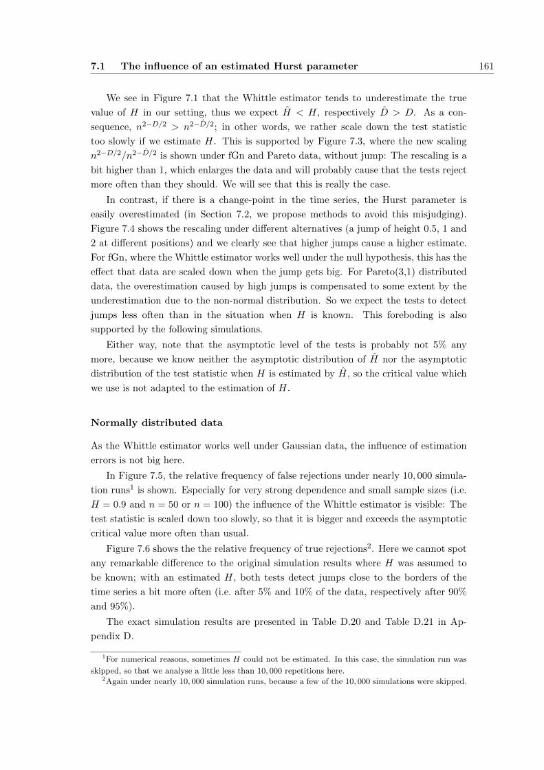
7.1 The influence of an estimated Hurst parameter 161
We see in Figure 7.1 that the Whittle estimator tends to underestimate the true
value of H in our setting, thus we expect H < H, respectively D > D. As a con-
sequence, n2−D/2 > n2−D/2; in other words, we rather scale down the test statistic
too slowly if we estimate H. This is supported by Figure 7.3, where the new scaling
n2−D/2/n2−D/2 is shown under fGn and Pareto data, without jump: The rescaling is a
bit higher than 1, which enlarges the data and will probably cause that the tests reject
more often than they should. We will see that this is really the case.
In contrast, if there is a change-point in the time series, the Hurst parameter is
easily overestimated (in Section 7.2, we propose methods to avoid this misjudging).
Figure 7.4 shows the rescaling under different alternatives (a jump of height 0.5, 1 and
2 at different positions) and we clearly see that higher jumps cause a higher estimate.
For fGn, where the Whittle estimator works well under the null hypothesis, this has the
effect that data are scaled down when the jump gets big. For Pareto(3,1) distributed
data, the overestimation caused by high jumps is compensated to some extent by the
underestimation due to the non-normal distribution. So we expect the tests to detect
jumps less often than in the situation when H is known. This foreboding is also
supported by the following simulations.
Either way, note that the asymptotic level of the tests is probably not 5% any
more, because we know neither the asymptotic distribution of H nor the asymptotic
distribution of the test statistic when H is estimated by H, so the critical value which
we use is not adapted to the estimation of H.
Normally distributed data
As the Whittle estimator works well under Gaussian data, the influence of estimation
errors is not big here.
In Figure 7.5, the relative frequency of false rejections under nearly 10, 000 simula-
tion runs1 is shown. Especially for very strong dependence and small sample sizes (i.e.
H = 0.9 and n = 50 or n = 100) the influence of the Whittle estimator is visible: The
test statistic is scaled down too slowly, so that it is bigger and exceeds the asymptotic
critical value more often than usual.
Figure 7.6 shows the the relative frequency of true rejections2. Here we cannot spot
any remarkable difference to the original simulation results where H was assumed to
be known; with an estimated H, both tests detect jumps close to the borders of the
time series a bit more often (i.e. after 5% and 10% of the data, respectively after 90%
and 95%).
The exact simulation results are presented in Table D.20 and Table D.21 in Ap-
pendix D.
1For numerical reasons, sometimes H could not be estimated. In this case, the simulation run was
skipped, so that we analyse a little less than 10, 000 repetitions here.2Again under nearly 10, 000 simulation runs, because a few of the 10, 000 simulations were skipped.
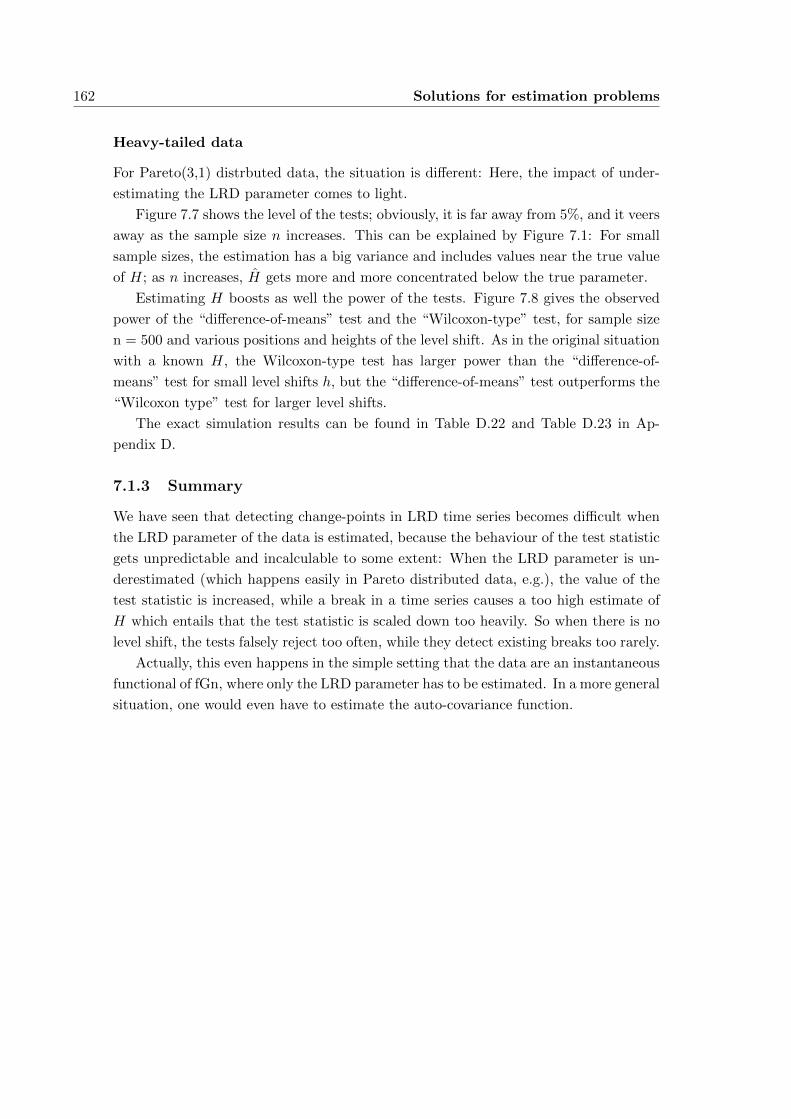
162 Solutions for estimation problems
Heavy-tailed data
For Pareto(3,1) distrbuted data, the situation is different: Here, the impact of under-
estimating the LRD parameter comes to light.
Figure 7.7 shows the level of the tests; obviously, it is far away from 5%, and it veers
away as the sample size n increases. This can be explained by Figure 7.1: For small
sample sizes, the estimation has a big variance and includes values near the true value
of H; as n increases, H gets more and more concentrated below the true parameter.
Estimating H boosts as well the power of the tests. Figure 7.8 gives the observed
power of the “difference-of-means” test and the “Wilcoxon-type” test, for sample size
n = 500 and various positions and heights of the level shift. As in the original situation
with a known H, the Wilcoxon-type test has larger power than the “difference-of-
means” test for small level shifts h, but the “difference-of-means” test outperforms the
“Wilcoxon type” test for larger level shifts.
The exact simulation results can be found in Table D.22 and Table D.23 in Ap-
pendix D.
7.1.3 Summary
We have seen that detecting change-points in LRD time series becomes difficult when
the LRD parameter of the data is estimated, because the behaviour of the test statistic
gets unpredictable and incalculable to some extent: When the LRD parameter is un-
derestimated (which happens easily in Pareto distributed data, e.g.), the value of the
test statistic is increased, while a break in a time series causes a too high estimate of
H which entails that the test statistic is scaled down too heavily. So when there is no
level shift, the tests falsely reject too often, while they detect existing breaks too rarely.
Actually, this even happens in the simple setting that the data are an instantaneous
functional of fGn, where only the LRD parameter has to be estimated. In a more general
situation, one would even have to estimate the auto-covariance function.
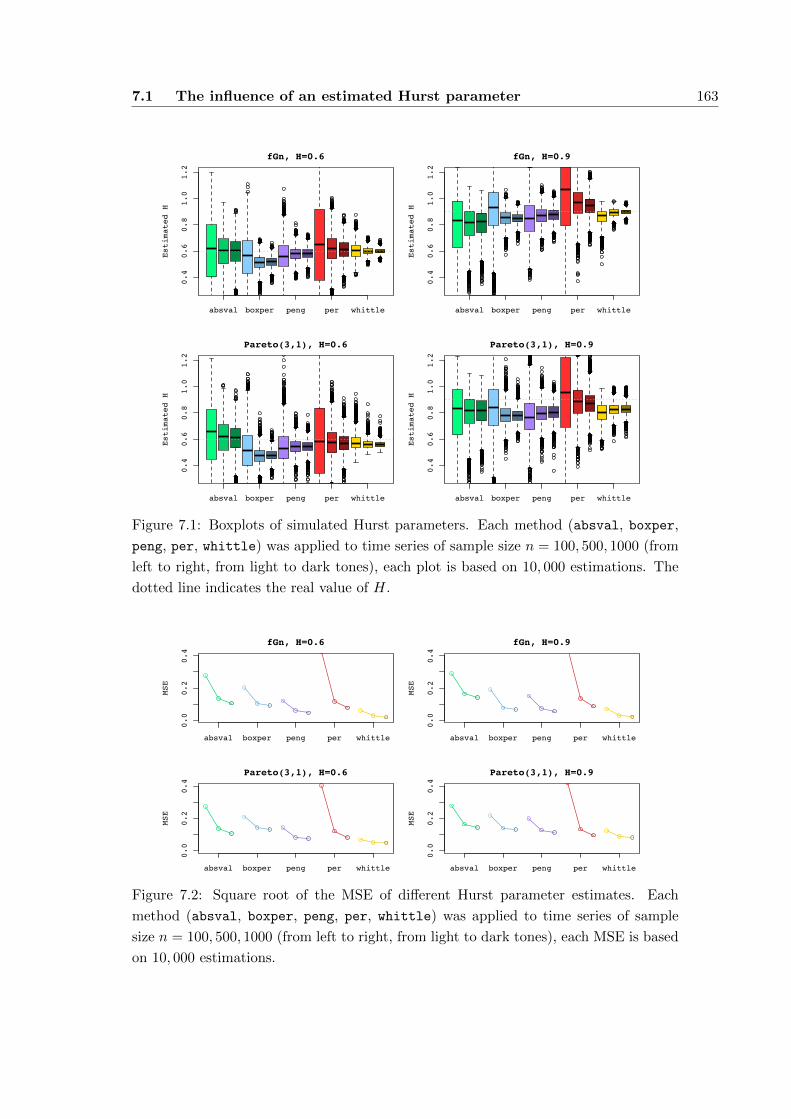
7.1 The influence of an estimated Hurst parameter 163
0.4
0.6
0.8
1.0
1.2
fGn, H=0.6Estimated H
absval boxper peng per whittle
0.4
0.6
0.8
1.0
1.2
fGn, H=0.9
Estimated H
absval boxper peng per whittle
0.4
0.6
0.8
1.0
1.2
Pareto(3,1), H=0.6
Estimated H
absval boxper peng per whittle
0.4
0.6
0.8
1.0
1.2
Pareto(3,1), H=0.9
Estimated H
absval boxper peng per whittle
Figure 7.1: Boxplots of simulated Hurst parameters. Each method (absval, boxper,
peng, per, whittle) was applied to time series of sample size n = 100, 500, 1000 (from
left to right, from light to dark tones), each plot is based on 10, 000 estimations. The
dotted line indicates the real value of H.
0.0
0.2
0.4
fGn, H=0.6
MSE
absval boxper peng per whittle
0.0
0.2
0.4
fGn, H=0.9
MSE
absval boxper peng per whittle
0.0
0.2
0.4
Pareto(3,1), H=0.6
MSE
absval boxper peng per whittle
0.0
0.2
0.4
Pareto(3,1), H=0.9
MSE
absval boxper peng per whittle
Figure 7.2: Square root of the MSE of different Hurst parameter estimates. Each
method (absval, boxper, peng, per, whittle) was applied to time series of sample
size n = 100, 500, 1000 (from left to right, from light to dark tones), each MSE is based
on 10, 000 estimations.
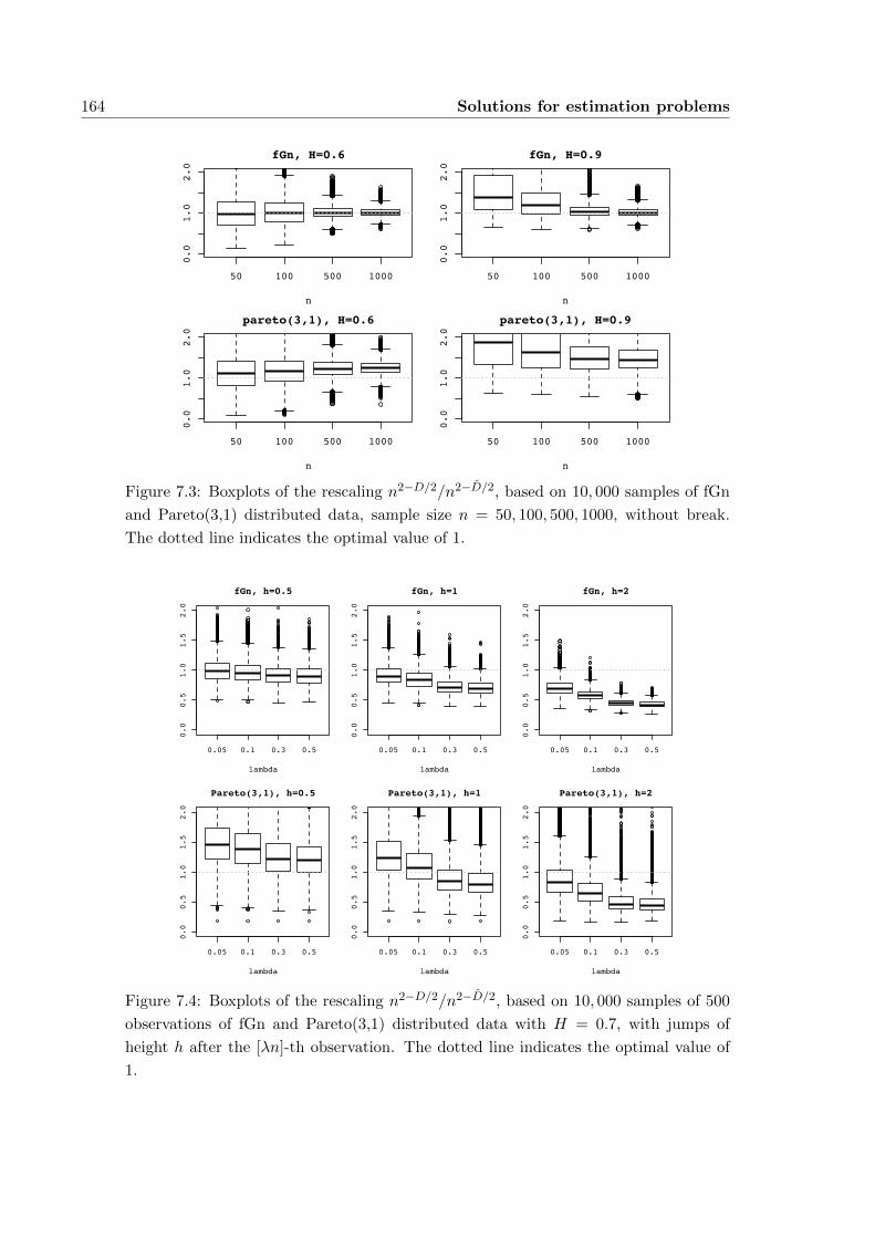
164 Solutions for estimation problems
50 100 500 1000
0.0
1.0
2.0
fGn, H=0.6
n
50 100 500 1000
0.0
1.0
2.0
fGn, H=0.9
n
50 100 500 1000
0.0
1.0
2.0
pareto(3,1), H=0.6
n
50 100 500 10000.0
1.0
2.0
pareto(3,1), H=0.9
n
Figure 7.3: Boxplots of the rescaling n2−D/2/n2−D/2, based on 10, 000 samples of fGn
and Pareto(3,1) distributed data, sample size n = 50, 100, 500, 1000, without break.
The dotted line indicates the optimal value of 1.
0.05 0.1 0.3 0.5
0.0
0.5
1.0
1.5
2.0
fGn, h=0.5
lambda
0.05 0.1 0.3 0.5
0.0
0.5
1.0
1.5
2.0
fGn, h=1
lambda
0.05 0.1 0.3 0.5
0.0
0.5
1.0
1.5
2.0
fGn, h=2
lambda
0.05 0.1 0.3 0.5
0.0
0.5
1.0
1.5
2.0
Pareto(3,1), h=0.5
lambda
0.05 0.1 0.3 0.5
0.0
0.5
1.0
1.5
2.0
Pareto(3,1), h=1
lambda
0.05 0.1 0.3 0.5
0.0
0.5
1.0
1.5
2.0
Pareto(3,1), h=2
lambda
Figure 7.4: Boxplots of the rescaling n2−D/2/n2−D/2, based on 10, 000 samples of 500
observations of fGn and Pareto(3,1) distributed data with H = 0.7, with jumps of
height h after the [λn]-th observation. The dotted line indicates the optimal value of
1.
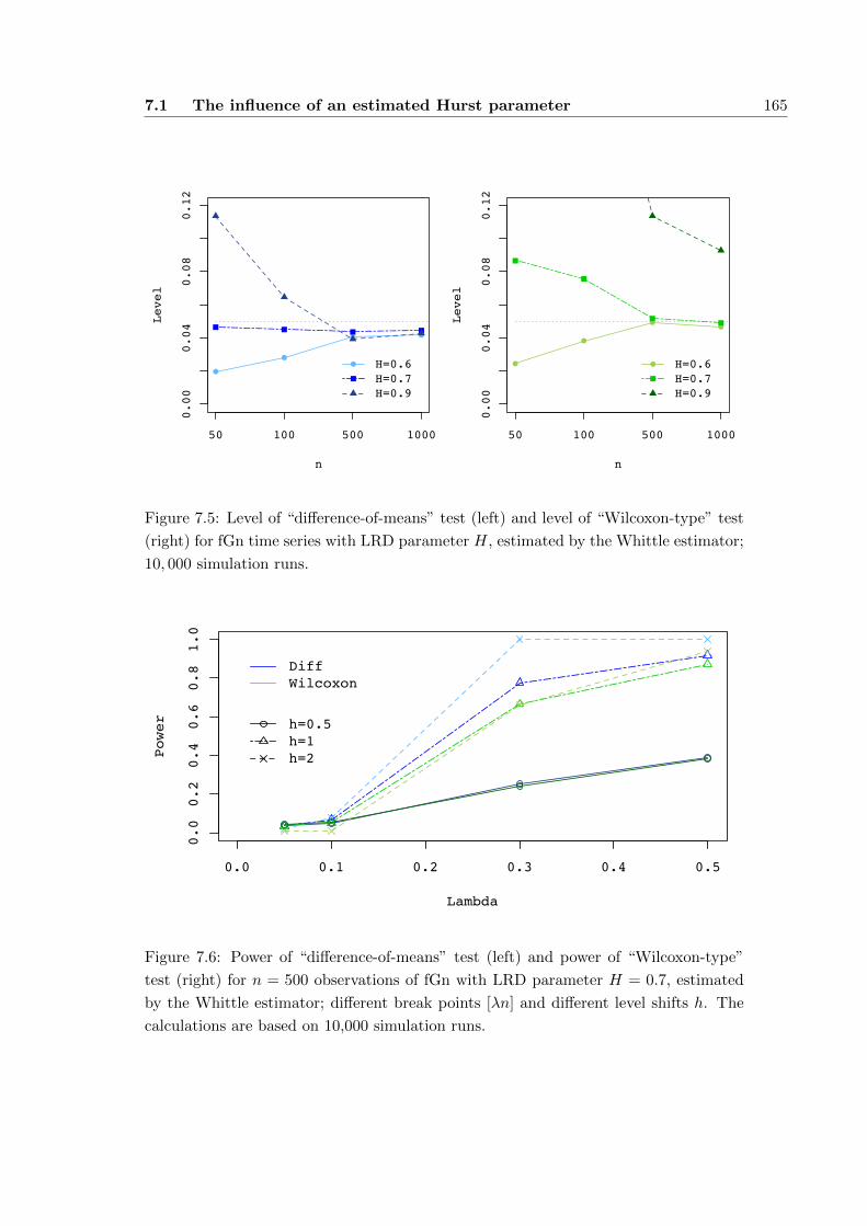
7.1 The influence of an estimated Hurst parameter 165
0.00
0.04
0.08
0.12
n
Level
50 100 500 1000
H=0.6H=0.7H=0.9
0.00
0.04
0.08
0.12
nLevel
50 100 500 1000
H=0.6H=0.7H=0.9
Figure 7.5: Level of “difference-of-means” test (left) and level of “Wilcoxon-type” test
(right) for fGn time series with LRD parameter H, estimated by the Whittle estimator;
10, 000 simulation runs.
0.0 0.1 0.2 0.3 0.4 0.5
0.0
0.2
0.4
0.6
0.8
1.0
Lambda
Power h=0.5
h=1h=2
DiffWilcoxon
Figure 7.6: Power of “difference-of-means” test (left) and power of “Wilcoxon-type”
test (right) for n = 500 observations of fGn with LRD parameter H = 0.7, estimated
by the Whittle estimator; different break points [λn] and different level shifts h. The
calculations are based on 10,000 simulation runs.
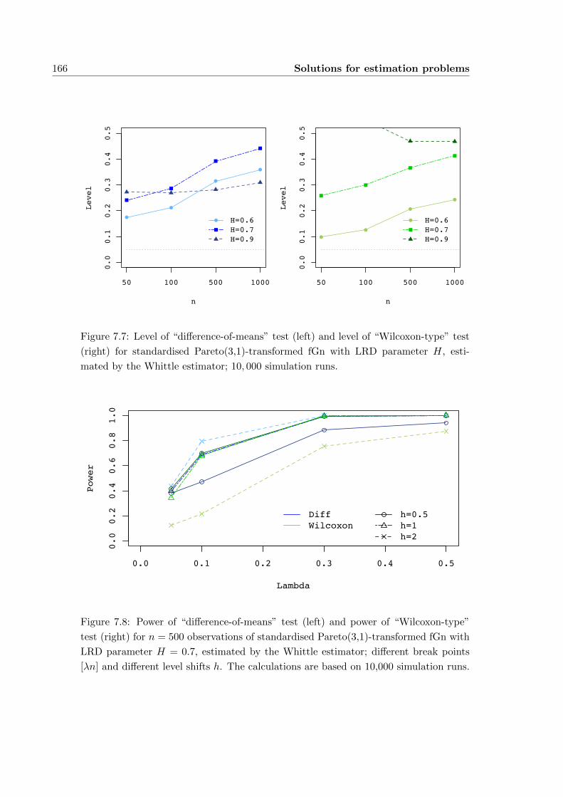
166 Solutions for estimation problems
0.0
0.1
0.2
0.3
0.4
0.5
n
Level
50 100 500 1000
H=0.6H=0.7H=0.9
0.0
0.1
0.2
0.3
0.4
0.5
n
Level
50 100 500 1000
H=0.6H=0.7H=0.9
Figure 7.7: Level of “difference-of-means” test (left) and level of “Wilcoxon-type” test
(right) for standardised Pareto(3,1)-transformed fGn with LRD parameter H, esti-
mated by the Whittle estimator; 10, 000 simulation runs.
0.0 0.1 0.2 0.3 0.4 0.5
0.0
0.2
0.4
0.6
0.8
1.0
Lambda
Power
h=0.5h=1h=2
DiffWilcoxon
Figure 7.8: Power of “difference-of-means” test (left) and power of “Wilcoxon-type”
test (right) for n = 500 observations of standardised Pareto(3,1)-transformed fGn with
LRD parameter H = 0.7, estimated by the Whittle estimator; different break points
[λn] and different level shifts h. The calculations are based on 10,000 simulation runs.
7.2 Estimating the LRD parameter under a change in the mean 167
7.2 Estimating the LRD parameter under a change in the
mean
There are several methods to estimate the LRD parameter. For an overview see the
articles by Taqqu, Teverovsky and Willinger (1995) and Taqqu and Teverovsky (1998).
But unfortunately, when one estimates H in order to apply a change-point test, one
maybe has to do with a time series that includes a jump (why else should one test
for it otherwise?), and such a jump intrinsically gets in the way of estimating the
LRD parameter since the usual estimators do not consider a change-point and likely
missspecify the resulting structure of the data as a more intense LRD. As a consequence,
the power of a change-point test likely decreases, because the jump may cause an
overestimation of H which may bring the test to interpret the jump as LRD behaviour.
We have just seen this effect in Section 7.1. Sibbertsen and Willert (2010) report that
tests for a break in persistence, i.e. a break in the long range-dependence structure,
are neither robust against a shift in the mean and must be adapted in this case. For
an overview about how structural breaks and trends lead to missspecification of LRD
and methods how to distinguish both effects, see the survey of Sibbertsen (2004) who
also points out that change-point estimators can not distinguish between LRD and
break points. Kramer, Sibbertsen and Kleiber (2002) illustrate this with data from the
German stock market, and Kramer and Sibbertsen (2002) show that in linear regression
models disturbances that exhibit LRD can be confused with structural changes.
It is thus a challenging problem to distinguish between behaviour that originates
from long memory and behaviour that originates from change-points. CUSUM-type
tests which discriminate between both, an LRD time series and a short-range dependent
time series with changes in the mean, have been proposed in the articles by Berkes et
al. (2006) and Shao (2011) which both contain a lot of references concerning LRD and
structural breaks. We focus on the situation where a LRD time series may possess a
change-point. In this situation, especially for change-point tests which usually require
the true, but unknown LRD parameter, there is a strong need for methods which
estimate the LRD parameter without being confused by the possible mean shift. Our
goal is thus to develop estimators for H which are on the one hand not heavily biased
by a jump in the mean of the data, but which on the other hand still work well if there
is no jump.
Kunsch (1987) and Hsu (2005) proposed usage of a local estimator to achieve this.
Hassler and Olivares (2007) applied such a method to German stock market data.
Kuswanto (2009) also analysed German stock market returns and used the invariance
of the LRD parameter under aggregation to develop an improved estimator of H by
looking at combinations of paired of aggregated series.
We propose a broader approach. We will develop and analyse three general methods
to estimate the LRD parameter in a time series which may include a jump that work
with any usual estimation technique. These adapted methods will prove to work better

168 Solutions for estimation problems
than the standard estimations which ignore jumps. All our methods have in common
that they base on the initial insight that, if it includes a jump, the whole LRD time
series is not appropriate for estimating the LRD parameter and that any estimation
approach must thus at first segregate the jump or concentrate on local environments
in the sample.
7.2.1 Adaption techniques
Seperating in two blocks
The first technique divides the time series into two blocks
X1, . . . , Xk and Xk+1, . . . , Xn
and estimates H on each block seperately. This is done for all possible cutting points.
Because the estimation of LRD intrinsically needs many observations, it is not sensible
if one allows early or late cutting points which produce a small block on which the
estimation of H is useless. We thus let the cutting point k take values in the set
K = klow, klow + 1, . . . , kup
with
klow = max[n/10], 10+ 1
kup = n− klow
and to end up to |K| = kup− klow + 1 pairs of estimations of H: for each cutting point
k ∈ K, we obtain an estimate H(1)k of H on the first block and an estimation H
(2)k of
H based on the second block.
As an estimate for the Hurst parameter of the whole sample, two functions of the
H(1)k , H
(2)k , k ∈ K are suitable: At first,
Hmean =1
|K|∑k∈K
H(1)k + H
(2)k
2
is the mean value of the estimate on the first and the second block, averaged over all
cutting points. Then,
Hmindiff =H
(1)k∗ + H
(2)k∗
2
with
k∗ = arg mink∈K
∣∣∣H(2)k − H
(1)k
∣∣∣is the mean value of the estimate on the first and the second block, diveded by the
special cutting point k∗ where both estimates differ least, measured by the absolute
difference.

7.2 Estimating the LRD parameter under a change in the mean 169
Estimating on a moving window
The second technique estimates H only on a part of the observations, on a certain
window
Xm−w, Xm−w+1, . . . , Xm, . . . , Xm+w
of length 2w + 1 around the center Xm. Now this window is moved through the time
series X1, . . . , Xn: For each m ∈ M = w + 1, w + 2, . . . , n − w, we estimate H on
the window around the midpoint Xm, and in doing so, we obtain finally |M | = n− 2w
estimates Hw,m for H.
We expect that for a fixed (and not too big) window size w, these estimates Hw,m,
m ∈ M , show a high variablilty because each estimation relies on a small window
which may include the jump or wich cover a rather steady part of the observations
(both resulting in too large estimation) or which may not include the jump or cover a
rather fluctuating section of the observations (both resulting in too low estimations) –
or a mixture of all these scenarios. Thus it seems reasonable to average all estimations
and consider
HMV,w =1
|M |∑m∈M
Hw,m
as an estimate for the true Hust parameter H.
In the context of blocks and windows for statistical inference, the choice of the
length of the block or window is traditionally an important issue. As flank length
w = w(n) as a function of the overall sample size n (which results in a window of size
2w + 1) we choose
w1 = w1(n) = max
[√n], 10
since the square root has often proven to be a good choice and since we do not want
the window to be too small as the estimation of an LRD parameter inherently gets bad
for a short sample of observations. For a comparison, we also analysed
w2 = w2(n) = max [n/10], 10
and
w3 = w3(n) = max [n/5], 10 .
Whenever moving window techniques are employed, it is much discussed if the
windows should be overlapping or non-overlapping. In our situation, the latter could
have the advantage that only one window of data is affected with the jump which results
in only one most likely erroneous estimate. So it is interesting (and a contribution to the
above discussion) to analyse also a non-overlapping moving window approach. Here,
H is estimated on blocks
X1, . . . , Xw, Xw+1, . . . , X2w, X2w+1, . . . , X3w, . . . X([N/w]−1)w+1, . . . , X[N/w]w
170 Solutions for estimation problems
of length w, resulting in [N/w] estimates Hw,k, k = 1, . . . , [N/w], for H. Again it is
reasonable to average and consider
HMV nl,w =1
[N/w]
[N/w]∑k=1
Hw,k
as an estimate for the true Hust parameter H. As window sizes, it is reasonable to
choose the same w1, w2, w3 as above. Since this method does not yield satisfying
results, for reasons of comparison, we only concentrated on window size w1 in the
following simulation study (see Section 7.2.2).
Pre-estimating the jump
Our third method is the most natural approach: Since the jump disturbes the estima-
tion of H, we try to remove it. For this purpose, we estimate the position and the
height of the jump, ignoring that we do not know the LRD parameter H yet, and then
either eliminate the jump and estimate H on the whole (now) jumpfree time series or
we estimate H on the observations before and on the observations after the jump and
take the mean value as an estimate for H on the overall sample.
We get down to details: Given the observations X1, . . . , Xn, we apply a change-
point test. In principle, we may take any change-point test we like. Here, we take the
“Wilcoxon-type” change-point test from Chapter 3 which rejects the null hypothesis
that there is no change in the mean for large values of the test statistic
max1≤k≤n−1
∣∣∣∣∣∣ 1
ndn
k∑i=1
n∑j=k+1
(IXi≤Xj −
1
2
)∣∣∣∣∣∣ . (7.1)
The change-point is supposed to take place after the observation Xk∗ for the k∗ ∈1, . . . , n − 1, for which the test statistic (7.1) takes its maximum value. Since the
scaling factor (ndn)−1 = n−2+D/2(c1L(n))−1/2 does not depend on k, it does not influ-
ence k∗. Knowledge about the LRD parameter H is therefore only essential for a test
decision if there is a change-point; the possible location k∗ is unaffected. This allows
us to pre-estimate the jump location without knowing H by
k∗ = arg max1≤k≤n−1
∣∣∣∣∣∣k∑i=1
n∑j=k+1
(IXi≤Xj −
1
2
)∣∣∣∣∣∣ . (7.2)
If there is a jump after X[τn] for a τ ∈ (0, 1), k∗ estimates its location [τn]; if there is
no jump in the time series, k∗ is some more or less meaningsless index in 1, . . . , n,but it will not affect the following estimation procedure.
Given the observations X1, . . . , Xn and an estimate k∗ for the jump location as
described in (7.2), we divide the observation into two parts
X1, . . . , Xk∗ and Xk∗+1, . . . , Xn.
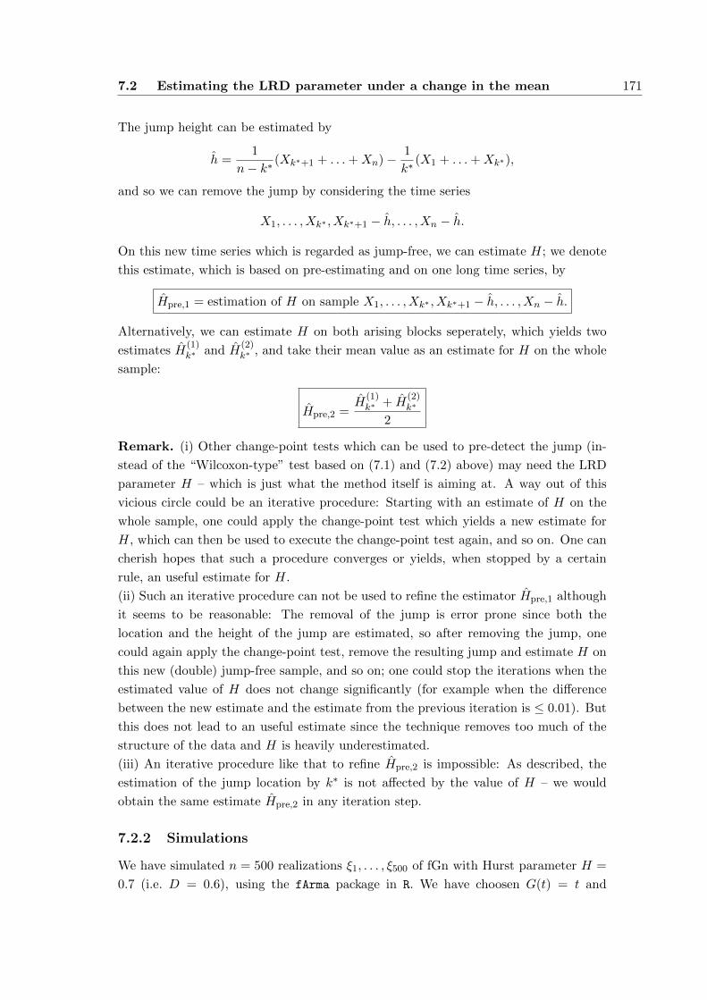
7.2 Estimating the LRD parameter under a change in the mean 171
The jump height can be estimated by
h =1
n− k∗(Xk∗+1 + . . .+Xn)− 1
k∗(X1 + . . .+Xk∗),
and so we can remove the jump by considering the time series
X1, . . . , Xk∗ , Xk∗+1 − h, . . . , Xn − h.
On this new time series which is regarded as jump-free, we can estimate H; we denote
this estimate, which is based on pre-estimating and on one long time series, by
Hpre,1 = estimation of H on sample X1, . . . , Xk∗ , Xk∗+1 − h, . . . , Xn − h.
Alternatively, we can estimate H on both arising blocks seperately, which yields two
estimates H(1)k∗ and H
(2)k∗ , and take their mean value as an estimate for H on the whole
sample:
Hpre,2 =H
(1)k∗ + H
(2)k∗
2
Remark. (i) Other change-point tests which can be used to pre-detect the jump (in-
stead of the “Wilcoxon-type” test based on (7.1) and (7.2) above) may need the LRD
parameter H – which is just what the method itself is aiming at. A way out of this
vicious circle could be an iterative procedure: Starting with an estimate of H on the
whole sample, one could apply the change-point test which yields a new estimate for
H, which can then be used to execute the change-point test again, and so on. One can
cherish hopes that such a procedure converges or yields, when stopped by a certain
rule, an useful estimate for H.
(ii) Such an iterative procedure can not be used to refine the estimator Hpre,1 although
it seems to be reasonable: The removal of the jump is error prone since both the
location and the height of the jump are estimated, so after removing the jump, one
could again apply the change-point test, remove the resulting jump and estimate H on
this new (double) jump-free sample, and so on; one could stop the iterations when the
estimated value of H does not change significantly (for example when the difference
between the new estimate and the estimate from the previous iteration is ≤ 0.01). But
this does not lead to an useful estimate since the technique removes too much of the
structure of the data and H is heavily underestimated.
(iii) An iterative procedure like that to refine Hpre,2 is impossible: As described, the
estimation of the jump location by k∗ is not affected by the value of H – we would
obtain the same estimate Hpre,2 in any iteration step.
7.2.2 Simulations
We have simulated n = 500 realizations ξ1, . . . , ξ500 of fGn with Hurst parameter H =
0.7 (i.e. D = 0.6), using the fArma package in R. We have choosen G(t) = t and

172 Solutions for estimation problems
obtained observations X1, . . . , X500 of fGn with H = 0.7. To this time series, we have
added a jump of height h = 0.5, 1, 2 after a proportion of λ = 0.1, 0.5 (i.e. after 50
and after 250 observations). To these resulting seven time series (one without jump,
six with jump at different positions and of different heights) we have applied each of
the above defined estimators, using exemplarily the Whittle Estimator (Section 7.2.2)
and the Box-Periodogram Estimator (Section 7.2.2) to estimate the value of the Hurst
parameter H = 1−D/2, see Taqqu, Teverovsky and Willinger (1995) and Giraitis and
Taqqu (1999). We have repeated these simulations 1, 000 times, so after all we obtained
1, 000 estimates H1 . . . , H1000 for each estimator H and each data situation.
Simulation results for the Whittle Estimator
In a first set of simulations, we have choosen the Whittle Estimator as generic estimation
method for H. In Table 7.1 the relative difference between the average of the above
described estimates H1 . . . , H1000 and the true parameter is given for each situation,
i.e. the valuemeanH1 . . . , H1000
H− 1
where H denotes the true parameter and H the respective estimate. For example,
for the usual estimator H (here: the Whittle estimator) and a jump of height 2 after
10% of the data (h = 2, λ = 0.1), we have tabulated 0.126 which means that in this
situation the usual estimator overestimates the true value on average by 12.6% (and
yields H = 0.788 as average estimate for the true parameter H = 0.7).
At a glance, we see that there is no uniformly best estimator; instead we observe
the following:
• For early or late jumps (λ = 0.1)
– and for small jump heights, the estimators Hmindiff, Hpre,1, HMV,w2 and
HMV,w3 yield the best results, while
– for high jumps, HMV,w1 is the best.
• For jumps in the middle (λ = 0.5)
– and for small jump heights, we obtain the best estimates with Hmean, Hpre,2
and HMV,w2 , while
– for high jumps, Hpre,2 and again HMV,w1 are the best.
• The non-overlapping moving window technique is worse than the regular (over-
lapping) moving window technique. We conjecture that this arises from under-
estimating H on small samples without jump and overestimating H on samples
with jump: In the non-overlapping technique, H is rather underestimated on
most of the few small windows, while in the regular overlapping technique, this
is compensated by rather overestimating H on all those many windows which
include the jump.
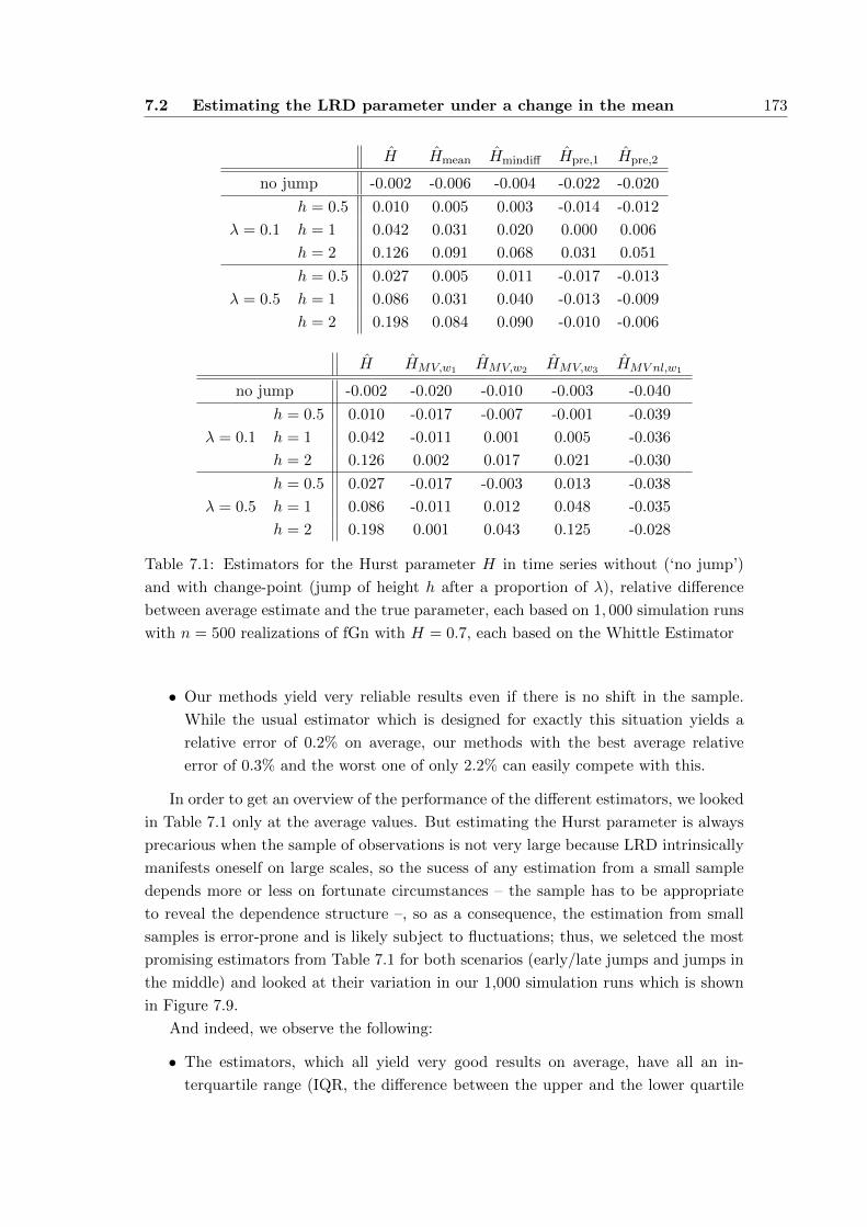
7.2 Estimating the LRD parameter under a change in the mean 173
H Hmean Hmindiff Hpre,1 Hpre,2
no jump -0.002 -0.006 -0.004 -0.022 -0.020
λ = 0.1
h = 0.5 0.010 0.005 0.003 -0.014 -0.012
h = 1 0.042 0.031 0.020 0.000 0.006
h = 2 0.126 0.091 0.068 0.031 0.051
λ = 0.5
h = 0.5 0.027 0.005 0.011 -0.017 -0.013
h = 1 0.086 0.031 0.040 -0.013 -0.009
h = 2 0.198 0.084 0.090 -0.010 -0.006
H HMV,w1 HMV,w2 HMV,w3 HMV nl,w1
no jump -0.002 -0.020 -0.010 -0.003 -0.040
λ = 0.1
h = 0.5 0.010 -0.017 -0.007 -0.001 -0.039
h = 1 0.042 -0.011 0.001 0.005 -0.036
h = 2 0.126 0.002 0.017 0.021 -0.030
λ = 0.5
h = 0.5 0.027 -0.017 -0.003 0.013 -0.038
h = 1 0.086 -0.011 0.012 0.048 -0.035
h = 2 0.198 0.001 0.043 0.125 -0.028
Table 7.1: Estimators for the Hurst parameter H in time series without (‘no jump’)
and with change-point (jump of height h after a proportion of λ), relative difference
between average estimate and the true parameter, each based on 1, 000 simulation runs
with n = 500 realizations of fGn with H = 0.7, each based on the Whittle Estimator
• Our methods yield very reliable results even if there is no shift in the sample.
While the usual estimator which is designed for exactly this situation yields a
relative error of 0.2% on average, our methods with the best average relative
error of 0.3% and the worst one of only 2.2% can easily compete with this.
In order to get an overview of the performance of the different estimators, we looked
in Table 7.1 only at the average values. But estimating the Hurst parameter is always
precarious when the sample of observations is not very large because LRD intrinsically
manifests oneself on large scales, so the sucess of any estimation from a small sample
depends more or less on fortunate circumstances – the sample has to be appropriate
to reveal the dependence structure –, so as a consequence, the estimation from small
samples is error-prone and is likely subject to fluctuations; thus, we seletced the most
promising estimators from Table 7.1 for both scenarios (early/late jumps and jumps in
the middle) and looked at their variation in our 1,000 simulation runs which is shown
in Figure 7.9.
And indeed, we observe the following:
• The estimators, which all yield very good results on average, have all an in-
terquartile range (IQR, the difference between the upper and the lower quartile

174 Solutions for estimation problems
of a sample) of around 0.04, in other words: half of all estimates (of the true
parameter H = 0.7) fluctuate between 0.66 and 0.74, which is pleasing.
• But the whiskers and outliers indicate that there are situations in which the
estimators miss the true value by up to around 0.1 – or even worse –, in other
words in which the estimation yields 0.6 or 0.8 instead of the true parameter value
H = 0.7.
• Taking into account the variability of the estimator, the moving window estimator
with the√n-window size, HMV,w1 , is uniformly the best in our survey: on average,
it yields good estimates, and the variation is not only rather constant over jump
heights and jump positions, but also one of the smallest among the analysed
estimators.
Simulation results for the Box-Periodogram Estimator
In a second set of simulations, we have choosen the Box-Periodogram Estimator as
underlying estimation method for H. In our simulation study, this estimator has proven
to be biased: it tends to underestimate the true value of H in time series without jump;
moreover, it has a bigger variance. In Table 7.2, again the relative difference between
the average of the above described estimates H1 . . . , H1000 and the true parameter is
given for each situation.
We observe clear differences to the simulations with the Whittle Estimator:
• In the high number of underestimations, even in time series with jump, the bias
of the underlying estimator becomes apparent.
• In combination with overestimating H when there is a jump in the mean, which
even slightly occurs when using our new jump-adapted estimation procedures,
this original bias causes that we sometimes obtain better results than with the
Whittle Estimator. This occurs here and there, but most likely for high jumps
(h = 1, h = 2) in the middle (λ = 0.5).
• Combined with the non-overlapping moving window approach HMV nl, the Box-
Periodogramm Estimator reveals a remarkable behaviour: it yields drasticly worse
results than the Box-Periodogramm Estimator without any modification. The
reason may be that, the larger the sample is, the more changes the bias of the
Box-Periodogramm Estimator from positive to negative as we have seen in our
inital simulation study. In the non-overlapping moving window approach, H is
estimated on only a few small windows, and on these, the Box-Periodogramm
Estimator yields impressive overestimations.
Again, we selected the most promising estimators from Table 7.2 for both scenarios
(early/late jumps and jumps in the middle) and looked at their variation; these are
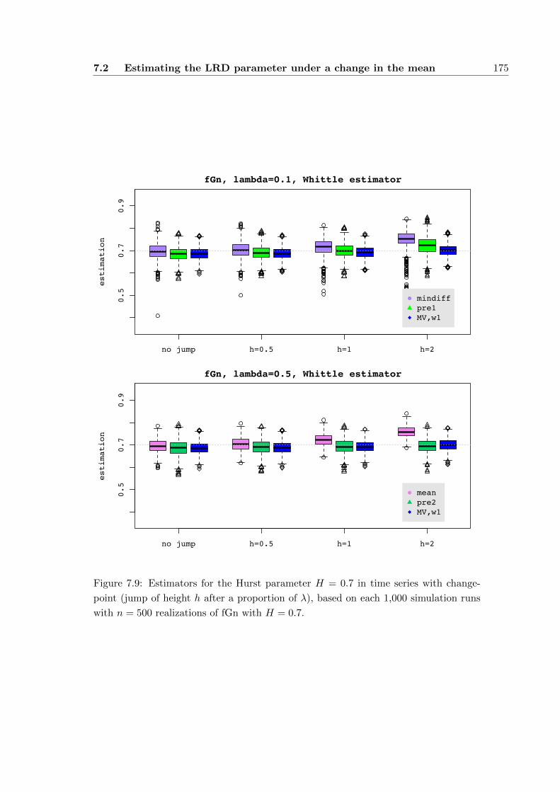
7.2 Estimating the LRD parameter under a change in the mean 175
fGn, lambda=0.1, Whittle estimator
estimation
no jump h=0.5 h=1 h=2
0.5
0.7
0.9
mindiffpre1MV,w1
fGn, lambda=0.5, Whittle estimator
estimation
no jump h=0.5 h=1 h=2
0.5
0.7
0.9
meanpre2MV,w1
Figure 7.9: Estimators for the Hurst parameter H = 0.7 in time series with change-
point (jump of height h after a proportion of λ), based on each 1,000 simulation runs
with n = 500 realizations of fGn with H = 0.7.
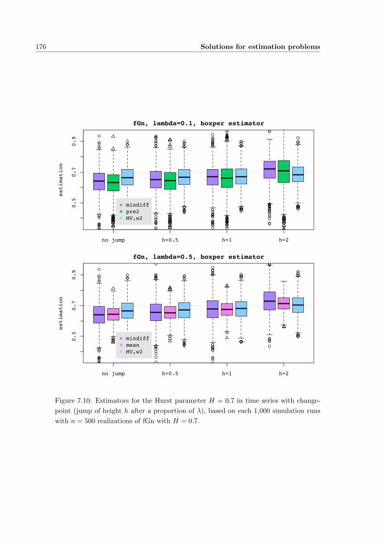
176 Solutions for estimation problems
fGn, lambda=0.1, boxper estimator
estimation
no jump h=0.5 h=1 h=2
0.5
0.7
0.9
mindiffpre2MV,w2
fGn, lambda=0.5, boxper estimator
estimation
no jump h=0.5 h=1 h=2
0.5
0.7
0.9
mindiffmeanMV,w2
Figure 7.10: Estimators for the Hurst parameter H = 0.7 in time series with change-
point (jump of height h after a proportion of λ), based on each 1,000 simulation runs
with n = 500 realizations of fGn with H = 0.7.
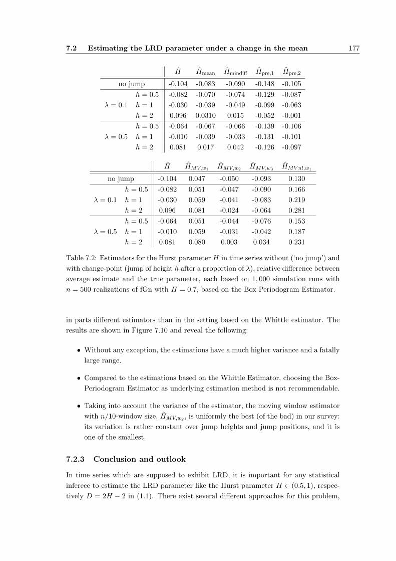
7.2 Estimating the LRD parameter under a change in the mean 177
H Hmean Hmindiff Hpre,1 Hpre,2
no jump -0.104 -0.083 -0.090 -0.148 -0.105
λ = 0.1
h = 0.5 -0.082 -0.070 -0.074 -0.129 -0.087
h = 1 -0.030 -0.039 -0.049 -0.099 -0.063
h = 2 0.096 0.0310 0.015 -0.052 -0.001
λ = 0.5
h = 0.5 -0.064 -0.067 -0.066 -0.139 -0.106
h = 1 -0.010 -0.039 -0.033 -0.131 -0.101
h = 2 0.081 0.017 0.042 -0.126 -0.097
H HMV,w1 HMV,w2 HMV,w3 HMV nl,w1
no jump -0.104 0.047 -0.050 -0.093 0.130
λ = 0.1
h = 0.5 -0.082 0.051 -0.047 -0.090 0.166
h = 1 -0.030 0.059 -0.041 -0.083 0.219
h = 2 0.096 0.081 -0.024 -0.064 0.281
λ = 0.5
h = 0.5 -0.064 0.051 -0.044 -0.076 0.153
h = 1 -0.010 0.059 -0.031 -0.042 0.187
h = 2 0.081 0.080 0.003 0.034 0.231
Table 7.2: Estimators for the Hurst parameter H in time series without (‘no jump’) and
with change-point (jump of height h after a proportion of λ), relative difference between
average estimate and the true parameter, each based on 1, 000 simulation runs with
n = 500 realizations of fGn with H = 0.7, based on the Box-Periodogram Estimator.
in parts different estimators than in the setting based on the Whittle estimator. The
results are shown in Figure 7.10 and reveal the following:
• Without any exception, the estimations have a much higher variance and a fatally
large range.
• Compared to the estimations based on the Whittle Estimator, choosing the Box-
Periodogram Estimator as underlying estimation method is not recommendable.
• Taking into account the variance of the estimator, the moving window estimator
with n/10-window size, HMV,w2 , is uniformly the best (of the bad) in our survey:
its variation is rather constant over jump heights and jump positions, and it is
one of the smallest.
7.2.3 Conclusion and outlook
In time series which are supposed to exhibit LRD, it is important for any statistical
inferece to estimate the LRD parameter like the Hurst parameter H ∈ (0.5, 1), respec-
tively D = 2H − 2 in (1.1). There exist several different approaches for this problem,

178 Solutions for estimation problems
but they all suffer from the defect that they are confused by structural changes in the
data: If there is a shift in the mean, the usual estimation methods easily missjudge
the structure of the data and may detect spurious or too heavy LRD. This drawback
is a fatal double bind when it comes to test for change-points in LRD time series:
Change-point tests naturally require knowledge of the Hurst parameter H in order
to discriminate between a change-point and behaviour which originates from the long
memory, but in practival situations, H must be estimated. Thus a jump in the data
may lead to overestimating H which may lead to overlooking the jump.
We have proposed three types of methods how estimation procedures can be adapted
in order to make allowance for even time series with a change in the mean. In a
simulation study we have compared these methods with different parameters and in
different jump-contaminated and also jump-free situations. Our research shows that
estimation of H can considerably be improved by our methods which yield better
estimates when there is a jump in the time series and which do not affect the estimation
when there is none.
It would be interesting to see how the proposed methods perform under different
data scenarios, e.g. heavy-tailed observations, which may occur if one chooses another
transormation G in our model, or a FARIMA model. Moreover, one could explore if one
could reach improvements by e.g. choosing other window sizes for the moving window
methods or by introducing weighted means for the methods which seperate the sample
in two blocks (instead of keeping the cutting point k away from the borders, one could
down-weight estimations where one of the blocks has a small size). It would also be
interesting to investigate how the methods can be adapted to allow for multiple breaks.
7.3 Estimating the first Hermite coefficient
The observations Xi = G(ξi) considered here exhibit LRD, and thus it is well-known
by now, but still astonishing, that the limit behaviour of the process
d−1n
[λn]∑i=1
Xi = d−1n
[λn]∑i=1
G(ξi), 0 ≤ λ ≤ 1,
only depends on very little properties of G, namely only on the Hermite rank of G
and the associated Hermite coefficient am (see Theorem 1.1): m determines the scaling
factor dn and the kind of limit distribution; am is a multiplicative factor in this limit
distribution. But this means: If one wants to do statistics based on the observations Xi,
e.g. the “difference-of-means” test from Section 3.4.2, one has to know the functionG, or
at least its Hermite rank and the belonging coefficient, otherwise the limit distribution
is unknown. Even in the comforting situation that G is strictly monotone in which
we already know by the Corollary to Theorem 3.5 that the “difference-of-means” test
statistic has always Hermite rank m = 1, we still need to know the first Hermite
coefficient a1. In what follows, we propose a method to estimate this Hermite coefficient
7.3 Estimating the first Hermite coefficient 179
if one only observes Xi = G(ξi), i = 1, . . . , n, for the broad class of strictly monotone
functions G.
7.3.1 The sort and replace method
For a start, we restrict ourselves to strictly monotonely increasing G. We want to
estimate the first Hermite coefficient
a1 := E[ξ G(ξ)],
where ξ ∼ N (0, 1). A natural way to estimate this expectation is the mean
a1 =1
n
n∑i=1
ξiG(ξi) =1
n
n∑i=1
ξiXi,
but this does not help since we do not observe the ξi. But here the monotonicity of G
comes in handy: We know that small Xi originate from small ξi and big Xi originate
from big ξi, so we sort the summands:
a1 =1
n
n∑i=1
ξiG(ξi) =1
n
n∑i=1
ξ(i)G(ξ(i)) =1
n
n∑i=1
ξ(i)X(i),
where in the last step we have essentially used that a strictly monotonely increasing G
does not change the order of the data. In order to estimate a1, we can now replace the
unknown ξi by new independent random variables ξ′i with the same distribution.
Theorem 7.1. Suppose that (ξi)i≥1 is a stationary Gaussian process with mean zero,
variance 1 and auto-covariance function (1.1) with 0 < D < 1. For G ∈ G2 define
Xk = G(ξk).
Let the Xk have a continuous c.d.f. F . Let ξ′i ∼ N (0, 1), i = 1, . . . , n, be i.i.d. random
variables, independent of the ξi that generate the observations Xi = G(ξi), as defined
above.
(i) If G is strictly monotonely increasing,
a1 :=1
n
n∑i=1
ξ′(i)X(i)P−→ a1. (7.3)
(ii) If G is strictly monotonely decreasing,
a1 :=1
n
n∑i=1
ξ′(i)X(n−i)P−→ a1. (7.4)
180 Solutions for estimation problems
Proof. (i) G is strictly increasing. G ∈ L2(R,N ) entails f(t) = tG(t) ∈ L1(R,N ), thus
by the ergodic theorem 1n
∑ni=1(ξiXi − a1)→ 0, almost surely. So it is to show that
1
n
n∑i=1
(ξ(i) − ξ′(i))X(i)P−→ 0.
By the Cauchy-Bunyakovsky-Schwarz inequality∣∣∣∣∣ 1nn∑i=1
(ξ(i) − ξ′(i))X(i)
∣∣∣∣∣ ≤√√√√ 1
n
n∑i=1
(ξ(i) − ξ′(i))2
√√√√ 1
n
n∑i=1
X2i ,
and the second factor converges to a constant, since G ∈ L2(R,N ). In order to show
that the first factor converges to zero, we truncate; set an arbitrary constant c > 0 and
define
ξi :=
−c if ξi < −c
c if ξi > c
ξi else
and ξ′i analogously. With Minkowski’s inequality and since truncation does not change
the order of the data, so that∑n
i=1(ξ(i) − ξ(i))2 =
∑ni=1(ξi − ξi)2, we obtain√√√√ 1
n
n∑i=1
(ξ(i) − ξ′(i))2 ≤
√√√√ 1
n
n∑i=1
(ξi − ξi)2 +
√√√√ 1
n
n∑i=1
(ξ′i − ξ′i)2 +
√√√√ 1
n
n∑i=1
(ξ(i) − ξ′(i))2.
(7.5)
The first term on the right-hand side of (7.5) vanishes asymptotically for n, c → ∞because √√√√ 1
n
n∑i=1
(ξi − ξi)2 n→∞−→√E[(ξi − ξi)2
]and E
[(ξi − ξi)2
]→ 0 as c→∞ due to the dominated convergence theorem, because
ξi − ξi → 0 and |ξi − ξi| < |ξi|. This holds of course for the second term in (7.5) as
well. We well now rigorously prove the intuition correct that for two samples ξ1, . . . , ξn
and ξ′1, . . . , ξ′n of identically distributed random variables ξ(i) gets close to ξ′(i), when n
increases. With |ξ(i) − ξ′(i)| ≤ 2c, we obtain for the last term on the right-hand side of
(7.5)
1
n
n∑i=1
(ξ(i) − ξ′(i))2 ≤ 2c max
i=1,...,n|ξ(i) − ξ′(i)|
≤ 2c maxi=1,...,n
(∣∣∣∣ξ(i) − Φ−1
(i
n
)∣∣∣∣+
∣∣∣∣ξ′(i) − Φ−1
(i
n
)∣∣∣∣) ,where Φ denotes the c.d.f of the single ξi. Note that by definition of ξi, Φ equals the
standard normal c.d.f. Φ on the interval (−c, c).
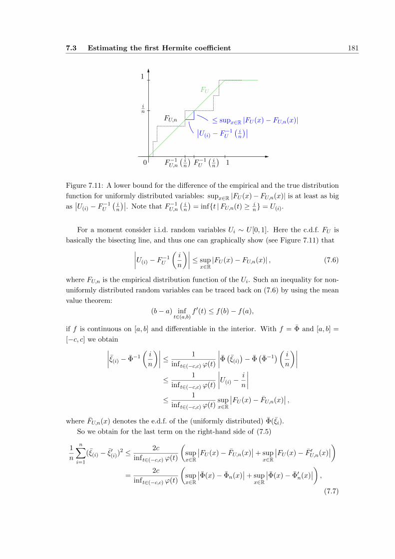
7.3 Estimating the first Hermite coefficient 181
0
1
FU
≤ supx∈R |FU (x)− FU,n(x)|∣∣U(i) − F−1U
(in
)∣∣FU,n
in
F−1U,n
(in
)F−1U
(in
)1
Figure 7.11: A lower bound for the difference of the empirical and the true distribution
function for uniformly distributed variables: supx∈R |FU (x)−FU,n(x)| is at least as big
as∣∣U(i) − F−1
U
(in
)∣∣. Note that F−1U,n
(in
)= inft |FU,n(t) ≥ i
n = U(i).
For a moment consider i.i.d. random variables Ui ∼ U [0, 1]. Here the c.d.f. FU is
basically the bisecting line, and thus one can graphically show (see Figure 7.11) that∣∣∣∣U(i) − F−1U
(i
n
)∣∣∣∣ ≤ supx∈R|FU (x)− FU,n(x)| , (7.6)
where FU,n is the empirical distribution function of the Ui. Such an inequality for non-
uniformly distributed random variables can be traced back on (7.6) by using the mean
value theorem:
(b− a) inft∈(a,b)
f ′(t) ≤ f(b)− f(a),
if f is continuous on [a, b] and differentiable in the interior. With f = Φ and [a, b] =
[−c, c] we obtain∣∣∣∣ξ(i) − Φ−1
(i
n
)∣∣∣∣ ≤ 1
inft∈(−c,c) ϕ(t)
∣∣∣∣Φ (ξ(i)
)− Φ
(Φ−1
)( in
)∣∣∣∣≤ 1
inft∈(−c,c) ϕ(t)
∣∣∣∣U(i) −i
n
∣∣∣∣≤ 1
inft∈(−c,c) ϕ(t)supx∈R
∣∣FU (x)− FU,n(x)∣∣ ,
where FU,n(x) denotes the e.d.f. of the (uniformly distributed) Φ(ξi).
So we obtain for the last term on the right-hand side of (7.5)
1
n
n∑i=1
(ξ(i) − ξ′(i))2 ≤ 2c
inft∈(−c,c) ϕ(t)
(supx∈R
∣∣FU (x)− FU,n(x)∣∣+ sup
x∈R
∣∣FU (x)− F ′U,n(x)∣∣)
=2c
inft∈(−c,c) ϕ(t)
(supx∈R
∣∣Φ(x)− Φn(x)∣∣+ sup
x∈R
∣∣Φ(x)− Φ′n(x)∣∣) ,
(7.7)
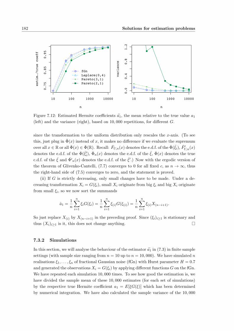
182 Solutions for estimation problems
0.75
0.85
0.95
n
estim./true coeff
10 100 1000 10000
fGnLaplace(0,4)Pareto(3,1)Pareto(2,1)
0.0
0.4
0.8
1.2
n
variance
10 100 1000 10000
Figure 7.12: Estimated Hermite coefficients a1, the mean relative to the true value a1
(left) and the variance (right), based on 10, 000 repetitions, for different G.
since the transformation to the uniform distribution only rescales the x-axis. (To see
this, just plug in Φ(x) instead of x, it makes no difference if we evaluate the supremum
over all x ∈ R or all Φ(x) ∈ Φ(R). Recall: FU,n(x) denotes the e.d.f. of the Φ(ξi), F′U,n(x)
denotes the e.d.f. of the Φ(ξ′i), Φn(x) denotes the e.d.f. of the ξ, Φ(x) denotes the true
c.d.f. of the ξ and Φ′n(x) denotes the e.d.f. of the ξ′.) Now with the ergodic version of
the theorem of Glivenko-Cantelli, (7.7) converges to 0 for all fixed c, as n → ∞, thus
the right-hand side of (7.5) converges to zero, and the statement is proved.
(ii) If G is strictly decreasing, only small changes have to be made. Under a de-
creasing transformation Xi = G(ξi), small Xi originate from big ξi and big Xi originate
from small ξi, so we now sort the summands
a1 =1
n
n∑i=1
ξiG(ξi) =1
n
n∑i=1
ξ(i)G(ξ(i)) =1
n
n∑i=1
ξ(i)X(n−i+1).
So just replace X(i) by X(n−i+1) in the preceding proof. Since (ξi)i≥1 is stationary and
thus (Xi)i≥1 is it, this does not change anything.
7.3.2 Simulations
In this section, we will analyse the behaviour of the estimator a1 in (7.3) in finite sample
settings (with sample size ranging from n = 10 up to n = 10, 000). We have simulated n
realisations ξ1, . . . , ξn of fractional Gaussian noise (fGn) with Hurst parameter H = 0.7
and generated the observationsXi = G(ξi) by applying different functionsG on the fGn.
We have repeated each simulation 10, 000 times. To see how good the estimation is, we
have divided the sample mean of these 10, 000 estimates (for each set of simulations)
by the respective true Hermite coefficient a1 = E[ξG(ξ)] which has been determined
by numerical integration. We have also calculated the sample variance of the 10, 000
7.3 Estimating the first Hermite coefficient 183
estimates. The simulation results are presented in Figure 7.12; the exact simulation
results are given in Table D.24 in Appendix D.
• Gaussian data.
With the increasing transformation G(t) = t we obtain standard fGn as oberva-
tions. This is the most simple non-trivial case in this model since G does not
change the underlying ξi. As one can expect, the estimation is very good in this
case.
• Symmetric data.
The function
G(t) = −(2−1/2) sgn
(Φ(t)− 1
2
)log
(1− 2
∣∣∣∣Φ(t)− 1
2
∣∣∣∣) .first transforms the data to a U [−1
2 ,12 ] distribution, then applies a quantile trans-
formation and finally centralises the data. This G is increasing and yields stan-
dardised Laplace(0,4) distributed data with p.d.f.
fst(x) =1√2
exp(−|√
2x|),
i.e. normal-tailed, symmetric data. G is a well-behaved transformation, so the
data are not too wild: The estimation is close to the Gaussian case.
• Not-so-heavy-tailed data.
A function G that provides heavy tails but a finite variance, so that it is coverd by
our techniques, is G(t) = (3/4)−1/2((Φ(t))−1/3 − 3
2
). G is decreasing and yields
standardised Pareto(3,1) distribution with p.d.f.
√3
4· f3,1
(√3
4x+
3
2
)=
3√
34
(√34 x+ 3
2
)−4
if x ≥ −√
13
0 else.
The estimated value is comparable to the estimated value under Pareto(2,1) data
(the case which we will treat next), but the variance of the estimation is fortu-
nately smaller.
• Heavy-tailed data.
G(t) = (Φ(t))−1/2 − 2 is decreasing and transforms the data to a centralised
Pareto(2,1)-distribution with p.d.f.
f2,1
(x+
3
2
)=
2(x+ 3
2
)−3if x ≥ −1
2
0 else.
So the Xi have heavy tails and and infinite variance. Note that such transfor-
mation G are actually not covered by Theorem 7.1, but it is interesting to study

184 Solutions for estimation problems
the performance of the estimator in such a case. Unsurprisingly, the estimation
is bad: For for small sample sizes, the mean is far away from the true value (al-
though it relies on 10,000 simulation runs), and the estimation is afflicted with a
huge variance.
Appendix A
A short introduction into
stochastic integration
In Section 1.3, I have mentioned (and we have seen it over and over throughout this
work) that the theory of LRD processes is strongly related to stochastic integration,
integration with respect to a stocastic process (instead of a deterministic function).
Now I will explain the idea behind these objects and their relation to LRD.
A.1 Wiener integral
The simplest stochastic integral is the Wiener integral
IW (f) =
∫ b
af(t) dB(t, ω),
where f is a deterministic function (i.e. it does not depend on ω) and B is a Brownian
motion. It can be constructed for arbitrary square-integrable functions f ∈ L2([a, b], λ)
by approximation procedures using step functions. To this end, divide the interval
[a, b] into n pieces: a = τ0 < τ1 < . . . < τn−1 < τn = b. For step functions f(t) =∑ni=1 aiI[τi−1,τi)(t), ai ∈ R, the integral is defined as
IW (f) =
n∑i=1
ai (B(τi)−B(τi−1)) .
Clearly, IW is a linear map on the space of step functions: IW (αf + βg) = αIW (f) +
βIW (g) for any α, β ∈ R and any step functions f, g. Using that the increments
B(t) − B(s) of a Brownian motion are independent N (0, t − s)-distributed, one can
easily show that
IW (f) ∼ N (0, σ2)
with
σ2 = E [IW (f)]2 =
∫ b
af2(t) dt.
186 A short introduction into stochastic integration
Now consider an arbitrary function f ∈ L2([a, b], λ) and choose a sequence (fn)n≥1 of
approximating step functions (i.e. fn → f). The last identity ensures that (IW (fn))n≥1
is a Cauchy sequence in L2 and thus converging. We define its limit as the Wiener
integral of f .
Definition A.1 (Wiener integral). For any f ∈ L2([a, b], λ), the Wiener integral of f
is
IW (f) = limn→∞
IW (fn),
where the convergence is in L2.
A Wiener integral has the following properties:
• The limit in the definition above is independent of the chosen approximating
sequence of step functions, such that IW (f) is well-defined.
• IW (f) =∫ ba f(t) dB(t, ω) is a Gaussian random variable with mean 0 and variance
‖f‖2 =∫ ba f
2(t) dt.
• From this it follows by some calculations that
E [IW (f)IW (g)] =
∫ b
af(t)g(t) dt,
and so, IW (F ) and IW (g) are independent, if f and g are orthogonal in L2([a, b], λ).
• The stochastic process
Mt =
∫ t
af(s) dB(s)
is a martingale.
Verifying these properties is not excessively difficult (Kuo, 2006, p. 9–21, gives
detailed proofs).
A.2 Ito integral
A natural question, at least for mathematicians, is now if one can define an integral
with respect to a Brownian motion even for stochastic processes as integrands. The
answer is positive; a so called Ito integral
II(f) =
∫ b
af(t, ω) dB(t, ω)
arises. Now f is a stochastic process, and this extension yields some severe problems.
If we want to keep the computationally advantageous martingale property, we need to
place some demands on f .
A.2 Ito integral 187
Definition A.2 (Adapted L2 space). Consider a probability space (Ω,F , P ). Let
L2ad([a, b]× Ω, λ× P ) be the class of functions
f(t, ω) : [a, b]× Ω→ R
such that
(i) (t, ω) 7→ f(t, ω) is B × F-measurable, where B denotes the Borel σ-algebra on
[a, b],
(ii) f(t, ω) is adapted to the filtration Ft, where Ft = σ(Bs, s ≤ t) is the σ-algebra
generated by the random variables Bs with s ≤ t (one can think of Ft as being
the history of Bs up to time t),
(iii) E[∫ ba f(t, ω)2 dt
]<∞.
For such processes f we can define a nice stochastic integral, and we will do this
once more by approximation procedures. At first, divide the interval [a, b] into n pieces
a = τ0 < τ1 < . . . < τn−1 < τn = b and consider a step process
f(t, ω) =
n∑i=1
ai(ω)I[τi−1,τi)(t),
where ai is now a Fτi−1-measurable, quadratically integrable random variable. For such
processes, the integral is defined as
II(f) =n∑i=1
ai(ω) (B(τi)−B(τi−1)) (ω).
Clearly, this is again linear: II(αf + βg) = αII(f) + βII(g) for any α, β ∈ R and
any step processes f, g. Not as easily as for Wiener integrals, one can show that
E [II(f)] = 0
E [II(f)]2 =
∫ b
aE [f(t, ω)]2 dt,
but of course II(f) is in general not normal distributed. This is a first raw version of
the so called Ito isometry.
With the aid of this isometry, one can extend the definition from step processes
to processes in L2ad([a, b] × Ω). At first, choose an arbitrary process g ∈ L2
ad which is
bounded and continuous in t for each ω. Then we can find an approximating sequence
(fn)n≥1 of step processes such that
E
[∫ b
a(g − fn)2 dt
]→ 0 as n→∞.
Next, one can approximate any bounded h ∈ L2ad by such bounded functions gn ∈ L2
ad
which are continuous in t for each fixed ω:
E
[∫ b
a(h− gn)2 dt
]→ 0 as n→∞
188 A short introduction into stochastic integration
Finally, we can approximate any arbitray f ∈ L2ad by bounded functions hn ∈ L2
ad:
E
[∫ b
a(f − hn)2 dt
]→ 0 as n→∞
The technical details of these approximations are worked out for example in the books
by Kuo (2006, Chap. 4.3) or Øksendal (1998, Chap. 3.1). These three steps together
mean that, in order to define an Ito integral, we can approximate any f ∈ L2ad by step
functions for which we have defined II(f).
Definition A.3 (Ito integral). For any f ∈ L2ad([a, b] × Ω, λ × P ), the Ito integral is
defined by
II(f) =
∫ b
af(t, ω) dBt(ω) = lim
n→∞II(fn),
where (fn)n≥1 is a sequence of step processes approximating f in L2([a, b]× Ω):
E
[∫ b
a(f(t, ω)− fn(t, ω))2 dt
]→ 0 as n→∞.
An Ito integral has the following properties:
• The limit in the definition above is independent of the chosen approximating
sequence of step processes, such that II(f) is well-defined.
• II(f) =∫ ba f(t, ω) dB(t, ω) is a random variable with mean 0 and variance
E
[∫ b
af(t, ω) dBt(ω)
]2
=
∫ b
aE[f2(t, ω)] dt
(this is called Ito isometry).
• For a sequence (fn)n≥1 ∈ L2ad with E
[∫ ba (f(t, ω)− fn(t, ω))2 dt
]→ 0 it holds
∫ b
afn(t, ω) dBt(ω)→
∫ b
af(t, ω) dBt(ω)
in L2(P ) as n→∞.
• For all f, g ∈ L2ad
E [II(f)II(g)] =
∫ b
aE [f(t, ω)g(t, ω)] dt.
•∫ ba f(t, ω) dBt(ω) is Fb-measurable.
• The stochastic process
Mt =
∫ t
af(s, ω) dBs(ω)
is a martingale with respect to the filtration Ft = σ(B(s), s ≤ t).
A.2 Ito integral 189
• Mt has a t-continuous version: There exists a t-continuous stochastic process Mt
on (Ω,F , P ) with P (Mt = Mt) = 1 for all t ∈ [a, b].
One major difference between stochastic and deterministic integrals is the follow-
ing: As usual, one approximates f(t, ω) by a step process∑
j f(t∗j , ω)I[tj−1,tj)(t) with
some t∗j ∈ [tj−1, tj), and the integral∫ ba f(t, ω) dBt(ω) is defined by the limit of∑
j f(t∗j , ω)(Btj − Btj−1). But what is now a bit surprising is that, in contrast to
Riemann integrals, it makes a difference which point t∗j ∈ [tj−1, tj) we choose, even
though the intervals become infinitely small.
Two choices have become common, for they have been proven useful: Choosing
the left endpoint of the interval t∗j = tj−1 leads to the Ito integral above, choosing
the mid-point t∗j = (tj−1 + tj)/2 leads to the so called Stratonovic integral. While
the Ito integral is a martingale and thus features some computational advantage, the
Stratonovich integral is not, however it behaves more pleasingly under transformations:
It allows for a chain rule without second order terms (which are inevitable for Ito in-
tegrals, see section A.3 below). Øksendal (1998, p. 36–37) gives a short discussion of
both concepts; Kuo (2006, Chap. 8.3) discusses the Stratonovich integral in the context
of Ito processes and the Ito formula (which we will shortly introduce).
It is possible to extend the definition of an Ito integral to a wider class of inte-
grands f . Condition (iii) in Definition A.2, E[∫ ba f(t, ω)2 dt] < ∞, can be relaxed to∫ b
a f(t, ω)2 dt <∞ a.s., which may be not integrable.
With the original definition, II(f) belongs to L2(Ω, P ), and since P is a probability
measure and therefore finite, it follows that II(f) ∈ L1(Ω, P ) as well, that means that
the Ito integral is an integrable random variable, and∫ ta f(s, ω)dBs(ω) is a martingale.
A function f that fulfills only the new condition∫ ba f(t, ω)2 dt <∞ a.s. does not neces-
sarily lead to an integrable II(f), and if it is not integrable, it cannot be a martingale.
But it is at least a so called local martingale which has as well a continuous version
(Kuo, 2006, Chap. 5).
In Definition A.2, condition (ii) can also be weakened. This allows to define multi-
dimensional Ito integrals and, as a special case, Ito integrals with respect to one single
coordinate of n-dimensional Brownian motion while the integrand is a function of other
of its coordinates. This is carried out by Øksendal (1998, Chap. 3.3) where some
bibliographical references are given as well. It is also possible to extend the definition
of an Ito integral to a wider class of integrators, namely to martingales. For f, g ∈L2
ad([a, b]× Ω) and a martingale Mt =∫ ta g(s, ω) dBs(ω) one defines
∫ b
af(t, ω) dMt(ω) =
∫ b
af(t, ω)g(t, ω) dBt(ω).
To obtain a useful definition, some further conditions on f are necessary; the con-
struction can be found in the book of Kuo (2006, Chap. 6), the essential tool is the
190 A short introduction into stochastic integration
Doob-Meyer decomposition.
As for ordinary random variables, we will ommit the argument ω when we deal with
stochastic processes if there is no danger of confusing something.
A.3 Ito process and Ito formula
As in ordinary calculus, one does not want to evaluate stochastic integrals by their
definition; it is laborious. But while ordinary integrals can be evaluated with the aid
of the fundamental theorem of calculus, with antiderivatives, such useful combination
of integration and differentiation is not on hand here, simply because in the world of
stochastic processes there is no differentiation. For example a chain rule like (f(g(t)))′ =
f ′(g(t))g′(t) in the context of processes,
(f(B(t)))′ = f ′(g(t))B′(t),
is meaningless since almost all sample paths of B(t) are nowhere differentiable. Nev-
ertheless, there is an analogue to the chain rule which lends us a hand at stochastic
integration.
Theorem A.1 (Ito formula I). For any f ∈ C2(R)
f(B(t))− f(B(a)) =
∫ t
af ′(B(s)) dB(s) +
1
2
∫ t
af ′′(B(s)) ds,
where the first summand on the right side is an Ito integral and the second one is an
ordinary Riemann integral for any sample path of B(s).
Obviously, the second term on the right side shows (or even constitutes) the differ-
ence between ordinary calculus in Newton/Leibnz sense and Ito calculus. It originates
in the Brownian motion which has a non zero quadratic variation. Using this simple
version of the Ito formula (or as well by calculating manually which is not too difficult
in this simple case), one obtains for example
1
2B2t =
1
2B2t −
1
2B2
0
=
∫ t
0Bs dB(s) +
1
2
∫ t
0ds
=
∫ t
0Bs dB(s) +
1
2t,
and this shows that a harmless transformation like g(x) = x2/2 converts an Ito integral
like Bt =∫ t
0 dBs in something which is not an Ito integral any more. Mathematicians
dislike such inconsistent behaviour, and so the need for another class of processes that
is stable under smooth transformations is obvious.
A.3 Ito process and Ito formula 191
Definition A.4 (Ito process). A stochastic process of the form
Xt(ω) = Xa(ω) +
∫ t
af(s, ω) dBs(ω) +
∫ t
ag(s, ω) ds, (A.1)
where Xa is Fa-measurable, a ≤ t ≤ b and f, g are in L2ad([a, b] × Ω) (or in the gener-
alisation of this space mentioned above) is called an Ito process. Often, such processes
are written in the convenient shorthand notation
dXt = f(t) dBt + g(t) dt, (A.2)
which is of course only a symbolic expression since the differential of B is not defined
because B is nowhere differentiable.
Bt =∫ t
0 dBs in the example above is an Ito process, and its transformation under
the map x 7→ x2/2 is it as well: It is the sum of a dBs- and a ds-integral. Its short
differential notation is
d
(1
2B2t
)= Bt dBt +
1
2dt.
Theorem A.2 (Ito formula II). For an Ito process Xt, as in (A.1) or (A.2), and a
function θ(t, x) ∈ C2([0,∞)× R),
Yt = θ(t,Xt)
is again an Ito process, and
θ(t,Xt) = θ(a,Xa) +
∫ t
a
∂θ
∂x(s,Xs)f(s) dBs
+
∫ t
a
(∂θ
∂t(s,Xs) +
∂θ
∂x(s,Xs)g(s) +
1
2
∂2θ
∂x2(s,Xs)f
2(s)
)ds
or in shorthand notation
dYt =∂θ
∂x(t,Xt) dXt +
∂θ
∂t(t,Xt) dt+
1
2
∂2θ
∂x2(t,Xt) (dXt)
2,
where (dXt)2 = (dXt) · (dXt) is computed by (A.2) and the symbolic multiplication
table1
× dBt dt
dBt dt 0
dt 0 0
.
Some important properties, extensions and applications are:
• With the aid of the Ito formula, a lot of stochastic integrals can be evaluated
using symbolic notation.
1Even not in full generality, Kuo (2006, p. 103) gives a nicely simple instruction how to use the
short notation and the multiplication table.
192 A short introduction into stochastic integration
• Ito processes and the Ito formula can be defined in the multi-dimensional case.
• The (multi-dimensional) Ito formula applies as well to processes with respect to
continuous and square integrable martingales (and not only with respect to the
Brownian motion).
• By the Ito formula, an integration by parts formula can be derived: If f is de-
terministic (that means f(s, ω) = f(s) only depends on s), continuous and of
bounded variation on [0, t], then∫ t
0 f(s) dBs = f(t)Bt −∫ t
0 Bs df(s).
• As stated above, an Ito integral is a martingale, but the converse is also true.
With the Ito formula, one can proove the important Martingale Representation
Theorem: Any martingale (adapted to Ft, with respect to the probability measure
P ) can be represented as an Ito integral.
A.4 Multiple Wiener-Ito integrals
As we have seen, we can find analogies between ordinary integration and stochastic
integration in many fields, but one obvious question remains: Can one define multiple
stochstic integrals? The answer is positive, but the construction of multiple stochstic
integrals is not self-evident. We restrict ourselfs to multiple Wiener integrals, i.e. to
deterministic integrands. The usual approach is to approximate such a deterministic
function f(t, s) by step functions
n∑i=1
m∑j=1
aijI[τi−1,τi)(t)I[si−1,si)(s),
where a = τ0 < τ1 < . . . < τn−1 < τn = b and a = s0 < s1 < . . . < sm−1 < sm = b are
partitions of the interval [a, b] and aij ∈ R. This construction yields for example∫ 1
0
∫ 1
01 dBt dBs = B2
1 ,
and this has the major drawback that it is unfortunately not orthogonal to constant
functions. In general, integrals of different degrees are by this approach, first introduced
by Wiener (1938), not orthogonal to each other.
Ito (1951) found a remedy (and this is why the construction is called multiple
Wiener-Ito integral): f has to be approximated by step functions which spare out the
diagonal of the domain of integration. For a start, we consider the two-dimensional
example above. Let ∆n = (τ0, . . . , τn) be a partition of the intervall [a, b] = [0, 1] into
n pieces. It naturally extends to a partition of the unit square
[0, 1)2 =
n⋃i,j=1
[τi−1, τi)× [τj−1, τj).
A.4 Multiple Wiener-Ito integrals 193
Defining step functions on this partition, where the interval in both dimensions is split
up in the same way, yields of course the same result as above because it is only a
special case of a general partition into rectangles: For the integrad f ≡ 1, we obtain
the Riemann sum
n∑i,j=1
(Bτi −Bτi−1)(Bτj −Bτj−1) =
(n∑i=1
(Bτi −Bτi−1)
)2
= B21 .
But now we remove the diagonal elements and evaluate the increments of the Brownian
motion over the domain
[0, 1)2\n⋃i=1
[τi−1, τi)2 =
⋃1≤i6=j≤n
[τi−1, τi)× [τj−1, τj),
i.e. the remaining off-diagonal squares:
Sn =∑
1≤i6=j≤n(Bτi −Bτi−1)(Bτj −Bτj−1)
=
n∑i,j=1
(Bτi −Bτi−1)(Bτj −Bτj−1)−n∑i=1
(Bτi −Bτi−1)2
→ B21 − 1 as ‖∆n‖ → 0
where ‖∆n‖ = max1≤i≤nτi − τi−1 is the fineness of the partition and where we have
used that the quadratic variation of the Brownian motion on an interval [a, b] is
lim‖∆n‖→0
n∑i=1
(Bτi −Bτi−1)2 = b− a,
see Kuo (2006, Th. 4.1.2). Thus∫ 1
01 dBt dBs = B2
1 − 1,
which is obviously orthogonal to a constant function.
This way of constructing multiple stochastic integrals has proved convenient. The
general construction for a dimension d ∈ N is as follows. Let [a, b] ⊂ R. A subset of
[a, b]d of the form [t(1)1 , t
(2)1 )× . . .× [t
(1)d , t
(2)d ) is called a rectangle. The diagonal set of
[a, b]d is the set D = (t1, . . . , td) ∈ [a, b]d | ∃i 6= j : ti = tj of all points which have at
least two identical coordinates.
Definition A.5 (Off-diagonal step function). A function
f(t1, . . . , td) =∑
1≤i1,...,id≤nai1,...,idI[τi1−1,τi1 )(t1) · · · I[τid−1,τid )(td)
on the rectangle [a, b]d with a partition a = τ0 < τ1 < . . . < τn = b in each dimension
is called a step function. It is called an off-diagonal step function if it vanishes on D,
that means if the coefficients satisfy
ai1,...,id = 0 if ip = iq for some p 6= q.
194 A short introduction into stochastic integration
The class of off-diagonal step functions is a vector space. For an off-diagonal step
function f define the d-dimensional multiple Wiener-Ito integral by
Id(f) =
∫[a,b]d
f(t1, . . . , td) dBt1 dBt2 · · · dBtd
=∑
1≤i1,...,id≤nai1,...,id ξi1ξi2 · · · ξid ,
where ξip = B(τip−1)−B(τip) is the increment of B over the p-th piece of the partition
of [a, b]. Note that the above representation of an off-diagonal step function is not
unique, but the multiple Wiener-Ito integral Id(f) is well-defined (it does not depend
on the representation of f). Again, Id(f) is linear on the vector space of off-diagonal
step functions.
Now note that we can write the diagonal set D as D =⋃
1≤i6=j≤d(D ∩ ti = tj),in other words: D is a finite union of intersections of D with (d − 1)-dimensional
hyperplanes. Thus, D is a set of the Lebesgue measure 0. This allows us to approximate
a function on [a, b]d by step functions on [a, b]d\D, i.e. by off-diagonal step functions,
because we can cover [a, b]d with rectangles that come arbitrarily close to the diagonal
set without touching it. So we summarize: For each f ∈ L2([a, b]d) we can find a
sequence (fn)n of off-diagonal step functions such that
limn→∞
∫[a,b]d|f(t1, . . . , td)− fn(t1, . . . , td)|2 dt1 dt2 · · · dtd = 0.
Definition A.6 (Symmetrization). Given a function f(t1, . . . , td), the symmetrization
of f is
f(t1, . . . , td) =1
d!
∑σ
f(tσ(1), . . . , tσ(d)),
where the sum is to be taken over all permutations σ of 1, 2, . . . , d.
If f is an off-diagonal step function, f is it as well. Since the Lebesgue measure
is symmetric, one can show that the multiple Wiener-Ito integrals based on f and f
coincide: Id(f) = Id(f). Moreover,
E [Id(f)]2 = d!
∫[a,b]d
|f(t1, . . . , td)|2 dt1 dt2 · · · dtd.
With this, we can proove for the above sequence (fn)n of off-diagonal step functions
that (Id(fn))n is a Cauchy sequence in L2(Ω) and therefore converging. The limit does
not not depend on the coice of the approximating sequence, so we can give
Definition A.7 (Multiple Wiener-Ito integral). For a function f ∈ L2([a, b]d), the
multiple Wiener-Ito integral Id(f) is defined by
Id(f) =
∫[a,b]d
f(t1, . . . , td) dBt1 dBt2 · · · dBtd := limn→∞
Id(fn),
where (fn)n is a sequence of off-diagonal step functions approximating f and the con-
vergence is in L2(Ω).
A.4 Multiple Wiener-Ito integrals 195
Multiple Wiener-Ito integrals have the following properties:
• It does not matter, if we integrate over f or its symmetrization f : Id(f) = Id(f).
• Id(f) is a random variable with expectation E[Id(f)] = 0 and variance E[Id(f)]2 =
d!‖f‖2, where ‖ · ‖ is the norm on L2([a, b]d).
• I1(f) is the simple Wiener integral.
• Multiple Wiener-Ito integrals of different orders are orthogonal: For n 6= m and
for any f ∈ L2([a, b]n), g ∈ L2([a, b]m) it holds E [In(f)Im(g)] = 0.
• To compute a multiple Wiener-Ito integral, it can be written as an iterated Ito
integral: ∫[a,b]d
f(t1, . . . , td) dBt1 dBt2 · · · dBtd
= d!
∫ b
a· · ·∫ td−2
a
(∫ td−1
af(t1, . . . , td) dBtd
)dBtd−1
· · · dBt1
A.4.1 Relation between Hermite polynomials and multiple Wiener-
Ito integrals
We will shortly illuminate the relation between Hermite polynomials and multiple
Wiener-Ito integrals. Let (Ω,F , P ) be a probability space and B(t) a Brownian mo-
tion with respect to P . Note that for a function f ∈ L2([a, b]), the Wiener integral∫ ba f(t) dB(t) is measurable with respect to the sigma field
FB := σ B(t) | a ≤ t ≤ b
which is smaller than F and in general not equal. Now let L2B(Ω) ⊂ L2(Ω) denote the
Hilbert space of P -square integrable functions on Ω which are mesurable with respect
to FB.
Define the tensor product of functions f1, . . . , fk ∈ L2([a, b]) as
f1 ⊗ · · · ⊗ fk(t1, . . . , tk) := f1(t1) · · · fk(tk).
The notation g⊗n11 ⊗ · · · ⊗ g⊗nkk means that gj is repeated nj times (1 ≤ j ≤ k); it is
a tensor product of n1 + . . . + nk factors. Now the Wiener-Ito integral of the tensor
product of f1, . . . , fk can be calculated as the product of some Hermite polynomials of
Wiener-Ito integrals of the single fj .
Theorem A.3. Let f1, . . . , fk be non-zero orthogonal functions in L2([a, b]) and n1, . . . , nk ∈N. Set n := n1 + . . .+ nk. Then
In(f⊗n1
1 ⊗ · · · ⊗ f⊗nkk
)=
k∏j=1
Hnj
(I(fj); ‖fj‖2
).
196 A short introduction into stochastic integration
And with this, one can show: Square integrable functions on Ω that are mesurable
with respect to FB can be represented as sum of multiple Wiener-Ito integrals:
Theorem A.4 (Wiener-Ito Theorem). The space L2B(Ω) can be decomposed into the
orthogonal direct sum
L2B(Ω) = K0 ⊕K1 ⊕K2 ⊕ . . . ,
where Kj consists of multiple Wiener-Ito integrals of order j. Each f ∈ L2B(Ω) has a
unique representation
f =∞∑j=0
Ij(fj)
with certain fj ∈ L2sym([a, b]j), the real Hilbert space of symmetric square integrable
functions on [a, b]j. Because of the orthogonality of Wiener-Ito integrals of different
order, we have
‖f‖2 =∞∑j=0
j! ‖fj‖2.
A proof and some comments on how to construct the before mentioned fj are given
by Kuo (2006, Chap. 9.7).
Appendix B
Additions
B.1 Proof of Theorem 2.3
As the Xi are jointly Gaussian with expectation 0, the numerator X − Y is an affine
linear transformation and therefore normally distributed with expectation 0 as well.
We only need to investigate its asymptotic variance.
For this purpose, we decompose the variance into three parts – one containing only
the variances of the first sample, one only containing these of the second sample and
one third including the interdependencies between both:
Var[X − Y ] =1
m2Var
[m∑i=1
Xi
]+
1
n2Var
[m+n∑i=m+1
Xi
]− 2
mn
m∑i=1
m+n∑j=m+1
Cov[Xi, Xj ]
=1
m2Var
[m∑i=1
Xi
]+
1
n2Var
[m+n∑i=m+1
Xi
]− 2
mn
m∑i=1
m+n−i∑j=m+1−i
γj (B.1)
=: A+B + C
Now we look into the convergence of each summand, starting with the last and most
difficult one.
Ad C. To detect the limiting behaviour we will replace some terms by other ones
that are asymptotically equivalent and easier to handle. For keeping an overview we will
at first show these replacements and give the detailed justification afterwards. During
198 Additions
the whole proof, all limits and asymptotic equivalences apply to an increasing overall
sample size N →∞ (and thus m,n→∞ as well).
m∑i=1
m+n−i∑j=m+1−i
γj =
m∑i=1
m+n−i∑j=1
γj −m−i∑j=1
γj
∼
m∑i=1
( c
Γ(2−D)(m+ n− i)1−DL(m+ n− i) (B.2)
− c
Γ(2−D)(m− i)1−DL(m− i)
)=
m+n−1∑k=1
c
Γ(2−D)k1−DL(k)−
n−1∑k=1
c
Γ(2−D)k1−DL(k) (B.3)
−m−1∑k=0
c
Γ(2−D)k1−DL(k)
∼ c
Γ(3−D)
((m+ n− 1)2−DL(m+ n− 1) (B.4)
− (n− 1)2−DL(n− 1)− (m− 1)2−DL(m− 1)
)
In (B.3) we have expanded the sum and changed the index of summation (in the first
sum m+ n− i = k, in the second sum m− i = k). Next we factor out (m+ n)2−D and
substitute m = λN and n = (1− λ)N .
m∑i=1
m+n−i∑j=m+1−i
γj ∼c
Γ(3−D)(m+ n)2−D
((N − 1
N
)2−DL(N − 1)
−(n− 1
N
)2−DL(n− 1)−
(m− 1
N
)2−DL(m− 1)
)∼ c
Γ(3−D)N2−DL(N)
(1− λ2−D − (1− λ)2−D) (B.5)
Now we give the promised justification of the asymptotic equivalences above. Look
at step (B.2). We apply Lemma 2.1 (iii) with
ai,m =
m+n−i∑j=1
γj −m−i∑j=1
γj
αi,m =c
Γ(2−D)
((m+ n− i)1−DL(m+ n− i)− (m− i)1−DL(m− i)
)= gm+n−i − gm−i.

B.1 Proof of Theorem 2.3 199
We have
m−1∑i=1
(ai,m − ai,m−1) + am,m =
m−1∑i=1
γm+n−i −m−1∑i=1
γm−i +
n∑i=1
γi
=m+n−1∑i=n+1
γi −m−1∑i=n+1
γi =m+n−1∑i=m
γi
and
m−1∑i=1
(αi,m − αi,m−1) + αm,m =
m−1∑i=1
(gm+n−i − gm−i − gm+n−i−1 − gm−i−1) + gn
=
m−1∑i=1
(gn+i − gi)−m−2∑i=0
(gn+i − gi) + gn
= gm+n−1 − gm−1.
We have to verify that these two expressions are asymptotically equivalent as m in-
creases. By (2.6) in Lemma 2.2
m+n−1∑i=1
γi ∼c(m+ n− 1)1−D
Γ(2−D)L(m+ n− 1) and
m−1∑i=1
γi ∼c(m− 1)1−D
Γ(2−D)L(m− 1),
and so by Lemma 2.1 (i),
m+n−1∑i=m
γi ∼c
Γ(2−D)
((m+ n− 1)1−DL(m+ n− 1)− (m− 1)1−DL(m− 1)
)= gm+n−1 − gm−1,
because
(m+ n− 1)1−DL(m+ n− 1)
(m− 1)1−DL(m− 1)∼(N
λN
)1−D L(N)
L(λN)→(
1
λ
)1−D> 1.
It remains to verify that∑m
k=1Dk,m is unbounded and strictly increasing. We shall see
that from some point the increments stay positive.
m∑i=1
αi,m −m−1∑i=1
αi,m−1
= gn +
m−1∑i=1
(gm+n−i − gm−i − gm−1+n−i + gm−1−i)
= gm+n−1 − gm−1
=c
Γ(2−D)
((m+ n− 1)1−DL(m+ n− 1)− (m− 1)1−DL(m− 1)
)=
c
Γ(2−D)(N − 1)1−DL(N − 1)
(1−
(λN − 1
N − 1
)1−D L(λN − 1)
L(N − 1)
)
200 Additions
Trivially, the first three factors are positive. The factor in brackets converges to
1 − λ1−D > 0, so it is positive for large N . Thus the sum in (B.2) is monotonic
from a certain index foreward. And we can see that the sum is unbounded: Its incre-
ments behave, at least from a certain index foreward and except a positive factor, like
N1−DL(N), in other words they are increasing.
Now look at step (B.4). The asymptotic equivalence of each single term is nothing
else than (2.6) with D − 1 instead of D (as noted in the proof, Karamata’s theorem
still holds as long D − 1 > −1); the asymptotic equivalence of all differences follows
similarly as before from Lemma 2.1 (i), since we have for the first difference
(N − 1)2−DL(N − 1)
((1− λ)N − 1)2−DL((1− λ)N − 1)∼(
1
1− λ
)2−D L(N)
L((1− λ)N)→(
1
1− λ
)2−D> 1
and for the second difference
(N − 1)2−DL(N − 1)− ((1− λ)N − 1)2−D L((1− λ)N − 1)
(λN − 1)2−DL(λN − 1)∼ 1− (1− λ)2−D
λ2−D
and recalling that D,λ ∈ (0, 1) we can bound this as follows:
1− (1− λ)2−D
λ2−D >1
λ2−(
1
λ− 1
)2
=2
λ− 1 > 2− 1 = 1.
Finally we deal with step (B.5). We have factored out L(N) and we have re-
placed L(N − 1)/L(N), L(n − 1)/L(N) and L(m − 1)/L(N) by 1 (this is equivalent
by Lemma 2.2 and since L is slowly varying). To ensure that we indeed are allowed
to make these replacements in the differences, we bring once more lemma 2.1 (i) into
action: 1/λ2−D > 1 for the first difference is trivial, and for the second difference we
have1− λ2−D
(1− λ)2−D >1− λ2−D
1− λ>
1− λ1− λ
= 1.
Ad A. Now that we coped with the covariances we confidently can tackle the
variances of X and Y .
Var
[m∑i=1
Xi
]=
m∑i=1
Var[Xi] +∑
1≤i6=j≤mCov[Xi, Xj ]
= mγ0 + 2
m−1∑k=1
(m− k)γk
Clearly,∑m−1
k=1 (m− k)γk =∑m
k=1mγk −∑m
k=1 kγk, and by (2.6) and by going through
the proof of Lemma 2.2 (ii), we obtain
m∑k=1
mγk ∼ cm2−D L(m)
Γ(2−D),
m∑k=1
kγk ∼ cm2−D L(m)
(2−D)Γ(1−D).

B.1 Proof of Theorem 2.3 201
Since
cm2−D L(m)
Γ(2−D)
/cm2−D L(m)
(2−D)Γ(1−D)=
2−D1−D
>1
1−D> 1,
we obtain with Lemma 2.1 (i)
m−1∑k=1
(m− k)γk ∼ cm2−D L(m)
Γ(2−D)
(1− 1−D
2−D
)= cm2−D L(m)
Γ(3−D). (B.6)
Now it is not a surprise that we apply Lemma 2.1 (i) one last time to detect finally
the asymptotic equivalence of mγ0 + 2∑m−1
k=1 (m− k)γk. Γ(3−D)γ0
/2cm1−DL(m)→
0 6= 1 is self-evident, so in the end we receive
Var
[m∑i=1
Xi
]∼ mγ0 + 2cm2−D L(m)
Γ(3−D). (B.7)
Ad B. Calculating the asymptotic variance of the sum of the Y ’s is exactly the
same as we just have done, so just replace m by n in the result:
Var
[m+n∑i=m+1
Xi
]= Var
[n∑i=1
Xi+m
]= nγ0 + 2
n−1∑k=1
(n− k)γk
∼ nγ0 + 2cn2−D L(n)
Γ(3−D)(B.8)
Now we look back on the decomposition (B.1) and put together the results on the
single summands (B.5), (B.7) and (B.8) to establish the asymptotic (expediently scaled)
variance of X − Y :
limN→∞
mn
(m+ n)2−D1
L(m+ n)Var
[X − Y
]= lim
N→∞
mn
(m+ n)2−D1
L(m+ n)
[1
m2mγ0 +
1
m22cm2−D L(m)
Γ(3−D)+
1
n2nγ0
+1
n22cn2−D L(n)
Γ(3−D)− 2
mn
c
Γ(3−D)N2−DL(N)
(1− λ2−D − (1− λ)2−D) ]
= limN→∞
λ(1− λ)
N−DL(N)
[γ0
λN+ 2cλ−DN−D
L(λN)
Γ(3−D)+
γ0
(1− λ)N
+ 2c(1− λ)−DN−DL((1− λ)N)
Γ(3−D)
− 2c
λ(1− λ)
1
Γ(3−D)N−DL(N)
(1− λ2−D − (1− λ)2−D) ]
=2c
Γ(3−D)λ(1− λ)
(λ−D + (1− λ)−D − 1− λ2−D − (1− λ)2−D
λ(1− λ)
)This completes the proof.
202 Additions
B.2 An heuristic example illustrating Theorem 2.3
We now make a check on Theorem 2.3 with an heuristic example. We consider γk = k−D
with D ∈ (0, 1) and disregard that this is actually not an auto-covariance function
(see the technical remark on page 25). We will calculate the asymptotic variance of√mn
(m+n)2−D (X−Y ) elementarily1. γk = γ(k) is monotonic decreasing and non-negative,
and a well known result from introductory analysis for decreasing f : R→ R≥0 is
∫ n+1
1f(x) dx ≤
n∑i=1
f(i) ≤∫ n
1f(x) dx+ f(1).
We will use this to replace sums by integrals (afterwards we ensure that the remainders
vanish asymptotically). As in the proof of Theorem 2.3, we analyse the single terms in
the decomposition (B.1).
m∑i=1
m+n−i∑j=m+1−i
γj =m∑i=1
m+n−i∑j=m+1−i
j−D (B.9)
≈m∑i=1
(∫ m+n−i
m+1−ij−D dj
)(B.10)
≈ 1
1−D
∫ m
i=1
((m+ n− i)1−D − (m+ 1− i)1−D) di (B.11)
≈ 1
1−D
∫ m
i=0
((m+ n− i)1−D − (m+ 1− i)1−D) di (B.12)
=(m+ n)2−D
(2−D)(1−D)
(1−
(m+ 1
m+ n
)2−D−(
n
m+ n
)2−D+
(1
m+ n
)2−D)
It is easy to see that
γ(m+ 1− i) = (m+ 1− i)−D = o((m+ n)2−D)∫ m+n−i+1
m+n−ij−D dj =
1
1−D((m+ n− i+ 1)1−D − (m+ n− i)1−D) = o
((m+ n)2−D) ,
so in (B.10) really holds “=” for large n (that is what we denoted by ≈), and the same
counts for (B.11). In (B.12) we have omitted the rest integral∫ 1
0
((m+ n− i)1−D − (m+ 1− i)1−D) di=
(m+ n)2−D
2−D
(1 +
(m
m+ n
)2−D−(m+ 1
m+ n
)2−D−(m+ n− 1
m+ n
)2−D)
=(m+ n)2−D
2−Do(1),
1We know by know that√nm/(n+m)2−D is the right scaling; but if we did not, we could sense it
in the course of the calculation.
B.3 Bounded variation in higher dimensions 203
so we have for the covariance term in (B.1):
limn→∞
mn
(m+ n)2−D1
mn
m∑i=1
m+n−i∑j=m+1−i
γj
= limn→∞
1
(1− D2 )(1−D)
(1−
(m+ 1
m+ n
)2−D−(
n
m+ n
)2−D+
(1
m+ n
)2−D)
=1
(1− D2 )(1−D)
(1− λ2−D − (1− λ)2−D) (B.13)
To detect the limiting behaviour of the two variance terms in (B.1), we use2 (1.8).
limN→∞
mn
(m+ n)2−D1
m2Var
[m∑i=1
Xi
]= lim
N→∞
λ(1− λ)
N−D(λN)−D
2
(1−D)(2−D)
= λ1−D(1− λ)2
(1−D)(2−D)(B.14)
limN→∞
mn
(m+ n)2−D1
n2Var
[n∑i=1
Xm+i
]= λ(1− λ)1−D 2
(1−D)(2−D)(B.15)
We now put together (B.13), (B.14), (B.15):
mn
(m+ n)2−D Var[X − Y
]N→∞−→ 1
(1− D2 )(1−D)
(λ1−D(1− λ) + λ(1− λ)1−D − 1 + λ2−D + (1− λ)2−D)
Alternatively, we may apply Theorem 2.3 with c = Γ(1−D) and L(k) ≡ 1. The result
is obviously the same.
B.3 Bounded variation in higher dimensions
In Chapter 3 we derived the limit distribution of the Wilcoxon two-sample test statistic
W[nλ],n =
[nλ]∑i=1
n∑j=[nλ]+1
IXi≤Xj, 0 ≤ λ ≤ 1.
Since W[nλ],n is a U -statistic, one could try to adapt the technique of Dehling and Taqqu
(1989) who treat one-sample U -statistics of LRD data in order to handle W[nλ],n; but
this approach fails since the kernel h(x, y) = Ix<y does not have bounded variation –
which is an essential technical requirement for the technique.
In this chapter, we will deal with the question what bounded variation is in higher
dimensions since it is of general interest, even though it does not lead to the desired
change-point test; we shall see that this is not trivial. At the end, we prove that
h(x, y) = Ix<y has (even locally) infinite variation.
2To draw on an existing limit theorem does of course not seem to be an “elementary” approach as
promised, but we do this only for reasons of speed; we could deduce the results in the same elementary
way as we have treated the rest of the calculation before.

204 Additions
B.3.1 Definition, properties and examples
Let f be a real valued function defined on a bounded interval [a, b] ⊂ R. The total
variation of f is defined by
‖f‖V,[a,b] := sup
p∑i=1
|f(ai)− f(ai−1)|,
where the supremum is taken over all finite sets of points ai | 0 ≤ i ≤ p < ∞ which
define a partition of the interval [a, b], i.e. with a = a0 < . . . < ap = b. If the underlying
interval [a, b] is clear, we shorty write ‖f‖V instead of ‖f‖V,[a,b]. If ‖f‖V < ∞ then f
is said to have bounded variation.
This one-dimensional variation has some nice properties (Kannan and Krueger
(1996, Chap. 6) provide proofs and some more results):
• If f is monotone, then ‖f‖V = |f(b)− f(a)| <∞.
• If f is Lipschitz continuous, then ‖f‖V <∞.
• If f has a bounded derivative, then ‖f‖V =∫ ba |f
′(x)| dx <∞.
• Sums, multiples and products of functions of bounded variation have itself bounded
variation: For functions f, g on [a, b] and a scalar α it holds ‖f + g‖V ≤ ‖f‖V +
‖g‖V , ‖αf‖V = |α|‖f‖V , and if ‖f‖V , ‖g‖V < ∞, then ‖fg‖V < ∞ (and the
same is true for f/g as long as |g(x)| ≥ c > 0 for all x ∈ [a, b]).
• The variation is additive: If [a, c] is divided by b ∈ (a, c), then ‖f‖V,[a,c] =
‖f‖V,[a,b] + ‖f‖V,[b,c].
• f is of bounded variation, if and only if it is the difference of two increasing,
bounded functions.
• If f has has bounded variation, then the left-hand limits f(x−) for x ∈ (a, b] and
the right-hand limits f(x+) for x ∈ [a, b) exist, f can have at most a countable
number of discontinuities, f ′ exists and is finite a.e..
The question is now how to define bounded variation for functions f : [a, b] ⊂Rd → R, d ≥ 2, and which properties hold for this higher-dimensional variation. Un-
fortunately, there is no obvious way to extend the definition of bounded variation to
several variables: Clarkson and Adams (1933) for example list six different definitions
of bounded variation for d = 2. We will take a closer look at two of them which proved
to be useful in the context of integration and measure; the first one is connected with
the names of Vitali, Lebesgue, Frechet and de la Vallee Poussin, the second one with
the names of Hardy and Krause. Owen (2004) discusses both definitions in detail in a
general setting (but with a notation that needs getting used to).
B.3 Bounded variation in higher dimensions 205
For a = (a1, . . . , ad), b = (b1, . . . , bd) ∈ Rd write a ≤ b, if the inequality holds for all
components (likewise define a < b). Define the hyperrectangle [a, b] ⊂ Rd as follows
[a, b] := x ∈ Rd | a ≤ x ≤ b
(and likewise (a, b], [a, b) and (a, b)). For f : [a, b] ⊂ Rd → R define the d-increment of
f over the rectangle R := [a, b] as
∆Rf :=∑
I⊂1,...,d
(−1)|I|f(xI),
where xI ∈ Rd has the components
(xI)i =
ai i ∈ I
bi i /∈ I.
Note that ∅ ⊂ 1, . . . d always. In case d = 1 this definition reduces to
∆Rf = f(b)− f(a) = f(b1)− f(a1),
in case d = 2 to
∆Rf = f(b1, b2)− f(b1, a2)− f(a1, b2) + f(a1, a2).
There are several ways to note down d-increments. Young (1916) for example defines
them recursively:
[f ]b1x1=a1= f(b1, x2,, . . . , xd)− f(a1, x2,, . . . , xd)
[f ]b1,b2x1=a1,x2=a2= [f(b1, x2,, . . . , xd)− f(a1, x2,, . . . , xd)]
b2x2=a2
...
[f ]b1,...,bda1,...,ad= ∆Rf
If it is clear over which rectangle the increments have to be computed, we will shortly
write ∆f instead of ∆Rf .
Definition B.1 (Monotonicity). A function f : Rd → R is called monotone, if ∆Rf ≥ 0
for all d-dimensional rectangles R.
Example. We consider some functions on the first quadrant R+×R+. By intuition we
expect f1(x, y) = x2y to be monotone because the functions x 7→ x2 and y 7→ y have
this property, and we expect f2(x, y) = −y sin(x) not to be monotone because the sinus
possesses hills and valleys – an educated guess. We compute the increments over the
rectangle [a1, b1]× [a2, b2] in the first quadrant R+ × R+ to verify this. The increment
∆f1 = f1(b1, b2)− f1(b1, a2)− f1(a1, b2) + f1(a1, a2)
= (b1 − a1)(b2 − a2)(a1 + b1)
206 Additions
is positive, so f1 is in fact monotone. The (sign of the) increment
∆f2 = (b2 − a2)(sin(a1)− sin(b1))
depends on the underlying rectangle (effectively, only the x-cordinates are crucial),
sin(a1) − sin(b1) can be negative, and so ∆f2 can be negative. f2 is therefore not
monotone.
But in general, more-dimensional monotonicity is not intuitively visible.
Example. We consider some monotone functions and take a closer look at their one-
and two-dimensional increments3 over the same rectangle as before. We will see that
their behaviour is quite different.
a) For f1(x, y) = x2y we have
∆f1 = (b1 − a1)(b2 − a2)(a1 + b1) > 0
∆xf1 = f1(b1, b2)− f1(a1, b2) = b2(b21 − a21) > 0
∆yf1 = f1(b1, b2)− f1(b1, a2) = b21(b2 − a2) > 0.
All increments in all dimensions are positive.
b) f3(x, y) = x4 − y5 does not look monotone. But it is:
∆f3 = 0
∆xf3 = b41 − a41 > 0
∆yf3 = a52 − b52 < 0
f3 is increasing in x and decreasing in y. Curiously, the 2-dimensional increment is
always 0. f4(x, y) = −y/x is an example of a function with the same 1-dimensional
properties, but an always positive 2-dimensional increment.
c) For f5(x, y) = e−xe−y we have
∆f5 = (eb1 − ea1)(eb2 − ea2)e−(a1+a2+b1+b2) > 0
∆xf5 = e−b2(e−b1 − e−a1) < 0
∆yf5 = e−b1(e−b2 − e−a2) < 0.
Although both 1-dimensional increments are negative, the 2-dimensional increment is
positive.
Definition B.2 (Vitali variation). For a function f : [a, b] ⊂ Rd → R let R be a finite
set of d-dimensional rectangles that exactly cover [a, b], i.e. R = Ri | 1 ≤ i ≤ p < ∞3When we consider one-dimensional increment, we will fix one argument and regard f(x, b2) and
f(b1, y) as functions of one variable. There is no deeper secret behind it that we fix the arguments just
to the upper bounds b1, b2; this is a convention in the notation of Hardy-Krause variation and it does
not matter which value in [ai, bi], i = 1, 2 we take.
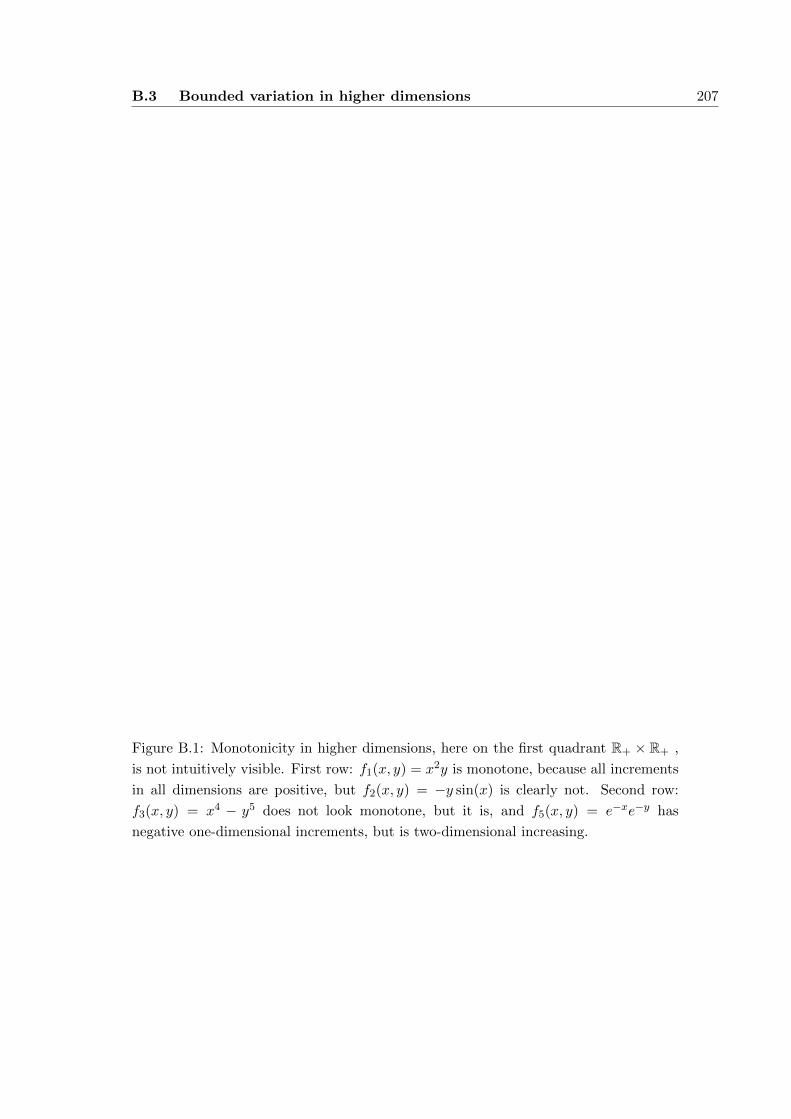
B.3 Bounded variation in higher dimensions 207
Figure B.1: Monotonicity in higher dimensions, here on the first quadrant R+ × R+ ,
is not intuitively visible. First row: f1(x, y) = x2y is monotone, because all increments
in all dimensions are positive, but f2(x, y) = −y sin(x) is clearly not. Second row:
f3(x, y) = x4 − y5 does not look monotone, but it is, and f5(x, y) = e−xe−y has
negative one-dimensional increments, but is two-dimensional increasing.

208 Additions
such that [a, b] =⋃pi=1Ri and the interiors of two different rectangles Ri, Rj are disjoint.
The Vitali variation of f is
‖f‖V,[a,b] := sup∑R∈R|∆Rf |, (B.16)
where the supremum is taken over all such sets R.
Clearly, for d = 1 this is the well-known standard definition of variation for real
functions on the real line which we considered at the beginning.
Definition B.3 (Hardy-Krause variation). Consider a function f : [a, b] ⊂ Rd → Rand a non-empty subset ∅ 6= I ⊂ 1, . . . , d. Define a new function fI :
∏i∈I [ai, bi]→ R
by setting the i-th argument of f equal to bi for all i /∈ I. The Hardy-Krause variation
of f is
‖f‖HK,[a,b] :=∑
∅6=I⊂1,...,d
‖fI‖V,[a,b]. (B.17)
For d = 1 the Hardy-Krause variation turns out to be the Vitali variation and
therefore the standard variation for real functions on the real line. In higher dimensions
both definitions differ, as we will shortly see.
Definition B.4 (Bounded variation). (i) f : [a, b] ⊂ Rd → R has bounded variation in
the sense of Vitali if
‖f‖V,[a,b] <∞.
The class of all such functions is denoted by BVV ([a, b]).
(ii) f : Rd → R has bounded variation in the sense of Vitali, if
sup‖f‖V,[a,b]
∣∣∣ [a, b] ⊂ Rd<∞.
Analogously we define bounded variation in Hardy-Krause sense. Denote the class of
functions with bounded Hardy-Krause variation by BVHK([a, b]).
Remark. A function is of bounded variation in Hardy-Krause sense if the sum over
all Vitali variations over [a, b] and its upper faces (bi is fixed as i-th argument) in all
dimension is bounded. Owen (2004) refers to Young (1913, p. 142) who proved that
this condition is equivalent to the original definition by Hardy (1905) that the sum is
bounded regardless of which point zi ∈ [ai, bi] we fix as i-th argument. We will make
use of this alternative definition later.
Now we collect some properties4 of functions on R2 which have bounded variation
in either Vitali or Hardy-Krause sense.
4A lot of results on bounded variation – in either way of defining it – does not hold in the same way
for all dimensions d. Keep in mind that Adams and Clarkson (1934) and Clarkson and Adams (1933)
only give proofs for d = 2 (it does not matter since we are interested just in two-dimensional results),
while Owen (2004) provides general results.
B.3 Bounded variation in higher dimensions 209
Proposition B.1. (i) BVV and BVHK are closed under + and −.
(ii) BVHK is closed under · and ÷ (as long as the quotient of two functions is defined),
but BVV is not.
(iii) If the rectangle R is split into subrectangles Ri, i = 1, . . . k, then
f ∈ BV (R) ⇒ f ∈ BV (Ri) ∀ = 1, . . . k,
and conversely
f ∈ BV (Ri) ∀ = 1, . . . k ⇒ f ∈ BV
(k⋃i=1
Ri
)
as long as⋃ki=1Ri is again a rectangle. This holds for both BVV and BVHK .
Proof. Owen (2004, Prop. 11) shows (i) and (ii), (iii) is demonstrated by Adams and
Clarkson (1934, Th. 11 and 12).
Proposition B.2. Let f be defined on [a, b] ⊂ R2.
(i)
f ∈ BVV ⇔ f = f1 − f2
where f1, f2 are functions with all 2-increments non-negative: ∆Rfi ≥ 0, i = 1, 2, for
all 2-dimensional rectangles R.
(ii)
f ∈ BVHK ⇔ f = f1 − f2
where f1, f2 are bounded functions with all increments non-negative: ∆Rfi ≥ 0, i = 1, 2,
for all rectangles R in all dimensions5, in other words ∆(f1)I ≥ 0 and ∆(f2)I ≥ 0 for
all I ⊂ 1, 2. In particular
f ∈ BVHK ⇒ f is bounded.
Proof. See Adams and Clarkson (1934, Th. 5 and 6).
These unequal representations of Vitali and Hardy-Krause variation reflect the dif-
ferences between both definitions: We expect the function f : [a1, b1]× [a2, b2]→ R,
f(x, y) =
1/(x− b1)2 x < b1
0 else,
not to have bounded variation, because it is not bounded. But surprisingly, it has
bounded Vitali variation, since the 2-increments are always 0. By the last proposition,
it can be written as f = f − 0, and f is not bounded. The notation of Hardy-Krause
variation does not suffer from this defect, it is a stronger property.
5In case d = 2, Young (1916) calls such functions with all increments non-negative “monotonely
monotone”.

210 Additions
Proposition B.3.
BVHK ⊂ BVVThe other implication is false in general.
Proof. f ∈ BVHK can be written as difference of two bounded functions with all incre-
ments non-negative. This is of course a difference of two functions with all 2-increments
non-negative, and therefore a function in BVV .
To prove the other implication wrong consider the Dirichlet function f(x, y) =
IQ(x). Although f has unbounded variation in x (note that it is even worse: it is
nowhere continuous in x), the 2-dimensional variation ∆f is always 0. So f ∈ BVV ,
but f /∈ BVHK .
Such examples can easily be constructed, as the following proposition shows.
Proposition B.4. If f : Rd → R does not depend on all d variables, then
‖f‖V = 0.
Proof. See Owen (2004, Prop. 8).
Technical remark. While BVV ⊂ BVHK is false in general, there are some further conditions we
can impose on f ∈ BVV to be as well in BVHK (Clarkson and Adams, 1933, p. 827, 841 and 846).
Proposition B.5. ‖ · ‖V and ‖ · ‖HK are semi-norms on functions.
Proof. This follows easily from the definitions. To see that they are not a norm, note
that both variations vanish for constant but non-zero functions.
B.3.2 The case h(x, y) = Ix≤y
One of the crucial points in the technique of Dehling and Taqqu (1989) is that h
must be of bounded variation. This condition is necessary to ensure that some terms
in the 2-dimensional integration by parts formula vanish at infinity, and above all it is
necessary to define∫∫
(Fm−F )(x)(Gn−G)(y) dh(x, y). Unfortunately, this requirement
is not met for many examples. This is, e.g., just the case for the kernel h(x, y) = Ix≤ywhich leads to the Mann-Whitney-Wilcoxon statistic. It has infinite variation (in Vitali
sense, and so as well in Hardy-Krause sense), even on compact domains if they cross
the diagonal D = (x, y) |x = y ⊂ R2.
To see this, consider h(x, y) = Ix≤y on an arbitrary rectangle R = [a, b] ⊂ R2
which crosses D. It is always possible to find another rectangle R′ ⊂ R inside which
touches the line D in such a way that three of its corners lie on the same side of D, see
Figure B.2. The 2-increment over R′ is 1, since the 2-increment of h over [a, b] is
∆Rh = h(b1, b2)− h(b1, a2)− h(a1, b2) + h(a1, a2)
and h can take values 0 and 1. Now it is always possible to divide R′ into three
subrectangles with the same property. In so doing, we obtain a partition of R with as
many subrectangles R with |∆Rh| = 1 as we wish.
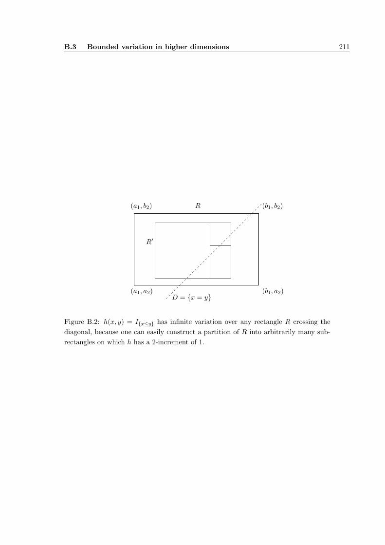
B.3 Bounded variation in higher dimensions 211
(a1, a2)
(a1, b2)
(b1, a2)
(b1, b2)R
R′
D = x = y
Figure B.2: h(x, y) = Ix≤y has infinite variation over any rectangle R crossing the
diagonal, because one can easily construct a partition of R into arbitrarily many sub-
rectangles on which h has a 2-increment of 1.

212 Additions

Appendix C
Source code of the simulations
C.1 Estimating the variance of X (section 2.4)
The routine varBlockmeans(x,r) estimates Var[X] of a time series X (which is given
as vector x and which has length N). The time series is divided in blocks of size r, the
mean values over these blocks is calculated and as the desired estimator, the sample
variance of these [N/r] block means is given out.
1 varBlockmeans <- function(x,r)
2 # x = given time series
3 # r = desired size of blocks
4 # r can be entered as absoulte size or relative to sample
size N
5 N = length(x)
6
7 # stop , if r has unfeasible values
8 if(r<=0 || r>N)
9 stop("Block size r must be positive and smaller than
the sample size (0 < r < N).")
10
11
12 # if block size r was entered as fractional amount of N,
convert it
13 if(r < 1)
14 r <- round(r*N)
15
16
17 # variance without Bessel ’s correction
18 varianz <- function(x) n=length(x) ; var(x) * (n-1) / n
19
20 if(r==1)
21 warning("Block size r = 1 means: The variance of the
single values in the time series is calculated (
variance of means over bocks of length 1).")

214 Source code of the simulations
22 varianz(x)
23
24 else
25 # divide x in blocks of length r
26 # Number of colums = integer part of N/r
27 nCols = N%/%r
28 # stop , if nCols < 2 (then variance of one single mean is
0)
29 if(nCols < 2)
30 stop("Only one block of the desired block size r could
be created from the time series x. The variance of
the block means (we have only one block!) is 0.")
31
32
33 Y = matrix(x[1:(r * nCols)], byrow = FALSE , ncol = nCols)
34
35 # colMeans := vector of means of N%/%r columns
36 varianz(colMeans(Y))
37
38
C.2 Estimating the auto-covariance (section 2.5)
This is just the standard estimator for the auto-covariances of a vector vect, as defined
in (2.18).
1 estimate.gamma <- function(vect)
2 N = length(vect)
3 gamma.dach = rep(NA , N-1)
4
5 for(h in 1:(N-1))
6 x.i = vect [1:(N-h)]
7 x.iplush = vect [(1:(N-h))+h]
8
9 # gamma.dach = 1/(N-h) sum_i=1^N-h X_iX_i+h
10 # i.e.\ sum(x.i*x.iplush)/(N-h)
11 gamma.dach[h] = mean(x.i*x.iplush)
12
13 gamma.dach
14
C.3 Estimating the variance of X − Y (section 2.6)
This program puts together the two last routines, as described in (2.22). It needs as
input the data sample vect, its Hurst parameter HH, the proportion llambda after

C.4 “Differences-of-means” test (section 3.6) 215
which the sample shall be divided, and the size rr of the blocks for the subroutine
varBlockmeans.
1 estimate.varXqYq <- function(vect , HH , llambda , rr)
2 alpha = 2-2*HH
3 D = alpha
4
5 N = length(vect)
6 m = floor(N*llambda)
7 n = N-m
8
9 # divide vect in m and N-m observation
10 x = vect [1:m]
11 y = vect[(m+1):N]
12
13 gamma_dach = estimate.gamma(vect)
14
15 # gamma_dach bad for large lags , so trim:
16 # set to 0 after 10*log10(N) observations
17 # this step may be commented out
18 maxlag = min(floor (10*log10(N)), N-1)
19 gamma_dach = c(gamma_dach [1: maxlag], rep(0, (N-1-maxlag))
)
20
21 # gamma_dach_sumoverj = sum_j = m+1-i^N-i, for i
=1,...,m
22 gamma_dach_sumoverj = rep(NA , m)
23
24 for(i in 1:m)
25 gamma_dach_sumoverj[i] = sum(gamma_dach[(m+1-i):(N-i)
])
26
27
28 estimator = (rr/m)^D * varBlockmeans(x, rr) + (rr/n)^D *
varBlockmeans(y, rr) - 2/(m*n) * sum(gamma_dach_
sumoverj)
29 estimator
30
C.4 “Differences-of-means” test (section 3.6)
The following program code calculates k repetitions of the “difference-of-means” test
statistic Dn, as defined in (3.16) for different sample lengths N and LRD parameter H.
The input needed is a N × k-matrix with k LRD time series of length N. The routine
is designed for time series with FGN; to apply it on other LRD series, one must adapt
the constants in the scaling dn.

216 Source code of the simulations
1 # function divides vector vec after entry with index cut
2 # and gives mean(x)-mean(y)
3 divide.and.difference <- function(vec , cut)
4 l = length(vec)
5 mean(vec [1: cut]) - mean(vec[(cut +1):l])
6
7
8 # function "calculate.Udiff" calculates U_diff =
9 # 1/(n dn) sum_i=1^ lambda n sum_j=lambda n + 1^n (Xi -
Xj)
10 # for two vectors X, Y (created by dividing one fGn series Z
)
11 # returns vector with 10.000 values of Udiff
12 # needs divide.and.difference
13 calculate.Udiff <- function(Z, cutpt , alpha)
14 # Z = given matrix of k fGn series (k columns of length N
)
15 # cutting point cutpt= 1,...,N-1
16
17 # error if cutting point not an integer number
18 if(cutpt - trunc(cutpt) != 0)
19 stop("Cutpoint is not an integer.")
20
21
22 # read dimensions of Z
23 N = nrow(Z)
24 k = ncol(Z)
25
26 # reserve vector U to store k values of Udiff
27 U = rep(NA ,k)
28
29 # cutting point should be in 1,2, ..., N-1
30 if(( cutpt >= 1) && (cutpt < N))
31 # apply "divide.and.difference" to columns of Z
32 # and write k results in vector U
33 U = apply(Z, 2, divide.and.difference , cut=cutpt)
34
35
36 # if cutpt out of range , T can ’t be calculated
37 if(( cutpt < 1) || (cutpt >= N))
38 U = rep(NA ,k)
39
40
41 lambd = cutpt/N
42
43 # fGn has covariances (1-alpha)(2-alpha)/2 k^(-alpha)
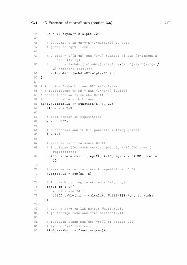
C.4 “Differences-of-means” test (section 3.6) 217
44 Lk = (1-alpha)*(2-alpha)/2
45
46 # constant c in dn=c*n^(1- alpha/2) is here
47 # just: c= sqrt (1/Lk)
48
49 # U_diff = 1/(n dn) sum_i=1^ lambda n sum_j=lambda n
+ 1^n (Xi-Xj)
50 # = lambda (1-lambda) n^( alpha/2) c^-1 L(n)^-1/
2 (mean(X)-mean(Y))
51 U = lambd*(1-lambd)*N^( alpha/2) * U
52
53
54 # function "make.k.times.DN" calculates
55 # k repetitions of DN = max_1<=k<N |Udiff|
56 # needs function calculate.Udiff
57 # output: table with k rows
58 make.k.times.DN <- function(H, N, Z)
59 alpha = 2-2*H
60
61 # read number of repetitions
62 k = ncol(Z)
63
64 # N observations => N-1 possible cutting points
65 l = N-1
66
67 # reserve marix to store Udiff
68 # l columns (for each cutting point), k=10.000 rows (
repetitions)
69 Udiff.table = matrix(rep(NA , k*l), byrow = FALSE , ncol =
l)
70
71 # reserve vector to store k repetitions of DN
72 k.times.DN = rep(NA , k)
73
74 # for each cutting point index i=1,...,N
75 for(i in 1:l)
76 # calculate Udiff
77 Udiff.table[,i] = calculate.Udiff(Z[1:N,], i, alpha)
78
79
80 # now we have an lxk matrix Udiff.table
81 # go through rows and find max(abs (..))
82
83 # function finds max(abs(vec)) of vector vec
84 # ignore "NA"-entries!
85 find.maxabs <- function(vec)
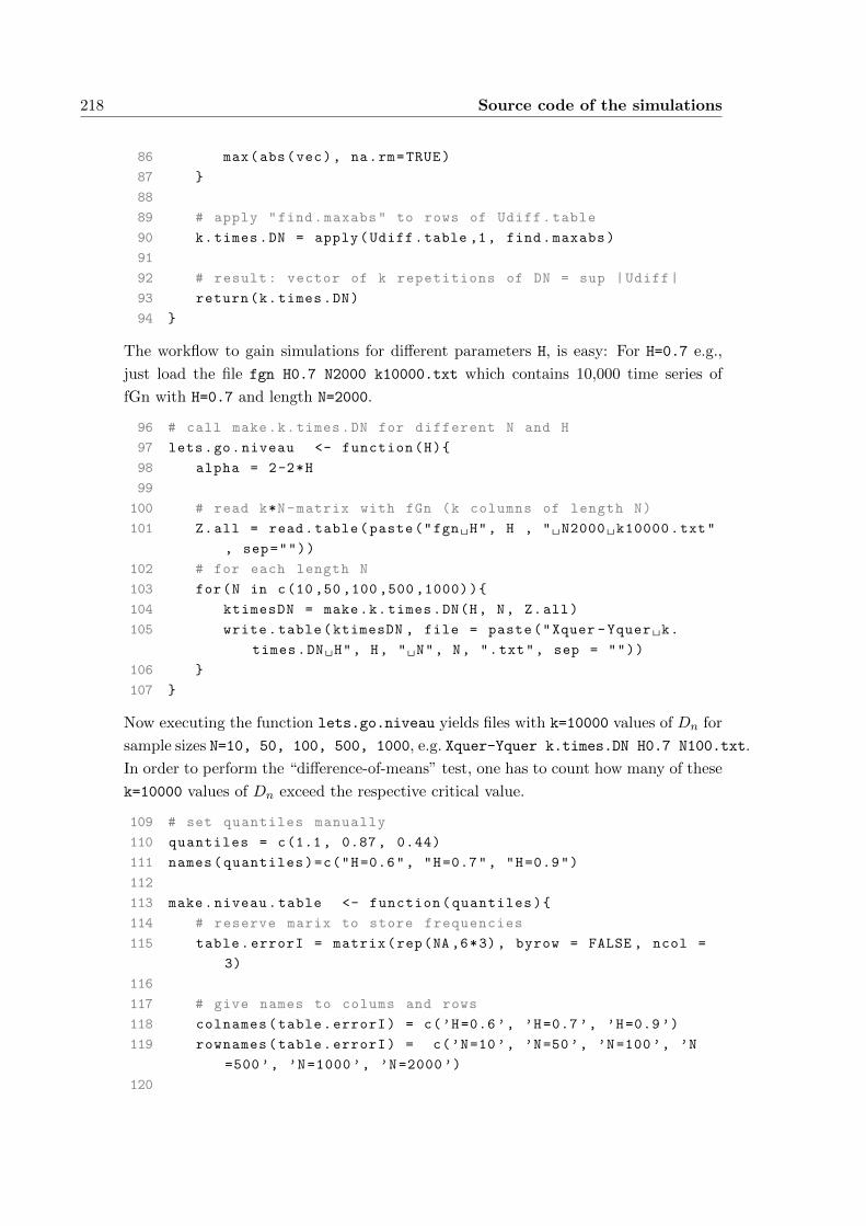
218 Source code of the simulations
86 max(abs(vec), na.rm=TRUE)
87
88
89 # apply "find.maxabs" to rows of Udiff.table
90 k.times.DN = apply(Udiff.table ,1, find.maxabs)
91
92 # result: vector of k repetitions of DN = sup |Udiff|
93 return(k.times.DN)
94
The workflow to gain simulations for different parameters H, is easy: For H=0.7 e.g.,
just load the file fgn H0.7 N2000 k10000.txt which contains 10,000 time series of
fGn with H=0.7 and length N=2000.
96 # call make.k.times.DN for different N and H
97 lets.go.niveau <- function(H)
98 alpha = 2-2*H
99
100 # read k*N-matrix with fGn (k columns of length N)
101 Z.all = read.table(paste("fgn H", H , " N2000 k10000.txt"
, sep=""))
102 # for each length N
103 for(N in c(10 ,50 ,100 ,500 ,1000))
104 ktimesDN = make.k.times.DN(H, N, Z.all)
105 write.table(ktimesDN , file = paste("Xquer -Yquer k.
times.DN H", H, " N", N, ".txt", sep = ""))
106
107
Now executing the function lets.go.niveau yields files with k=10000 values of Dn for
sample sizes N=10, 50, 100, 500, 1000, e.g. Xquer-Yquer k.times.DN H0.7 N100.txt.
In order to perform the “difference-of-means” test, one has to count how many of these
k=10000 values of Dn exceed the respective critical value.
109 # set quantiles manually
110 quantiles = c(1.1, 0.87, 0.44)
111 names(quantiles)=c("H=0.6", "H=0.7", "H=0.9")
112
113 make.niveau.table <- function(quantiles)
114 # reserve marix to store frequencies
115 table.errorI = matrix(rep(NA ,6*3), byrow = FALSE , ncol =
3)
116
117 # give names to colums and rows
118 colnames(table.errorI) = c(’H=0.6’, ’H=0.7’, ’H=0.9’)
119 rownames(table.errorI) = c(’N=10’, ’N=50’, ’N=100’, ’N
=500’, ’N=1000’, ’N=2000’)
120

C.4 “Differences-of-means” test (section 3.6) 219
121 # for each LRD parameter
122 for(H in c(0.6, 0.7, 0.9))
123 alpha = 2-2*H
124 # and for each length N=50, ..., N=2000
125 for(N in c(10 ,50 ,100 ,500 ,1000))
126 # read the simulation output Dn
127 dn = read.table(paste("Xquer -Yquer k.times.DN H", H
, " N", N, ".txt", sep=""))
128
129 # extract data (as vector) from data.frame T
130 dn = dn[,1]
131
132 table.errorI[paste("N=", N, sep=""),paste("H=", H,
sep="")] = length(which(dn > quantiles[ paste(
"H=", H, sep="")]))/length(dn)
133
134
135
136 table.errorI.rounded = round(table.errorI ,3)
137 write.table(table.errorI ,file="Tabelle Niveau Xq -Yq fGn.
txt")
138 write.table(table.errorI.rounded ,file="Tabelle Niveau Xq -
Yq fGn.txt",append=TRUE)
139
140
141 # make.niveau.table(quantiles)
The function make.niveau.table takes three critical values for H=0.6, 0.7, 0.9 and
yields a table with the observed level for each H and each sample size N, i.e. the relative
frequency of wrong rejections among the 10,000 simulation runs.
Now the routine to simulate the level of the test under various alternatives needs
the above defined functions calculate.Udiff and make.k.times.DN and an additional
function which adds a jump to the time series.
1 # function adds break -point of heigth hh
2 # at position lambda to a vector
3 add.break <- function(vec , lambd , hh)
4 ll = length(vec)
5 m = floor(lambd*ll)
6 vec.neu = c(vec [1:m], vec[(m+1):ll] + hh)
7 vec.neu
8
9
10 # now the workflow:
11 # call make.k.times.DN for different h and lambda
12 # to save simulation time: fix H and N
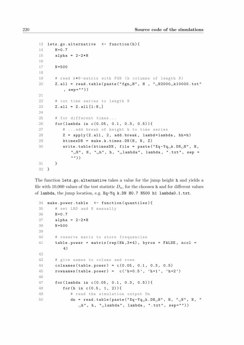
220 Source code of the simulations
13 lets.go.alternative <- function(h)
14 H=0.7
15 alpha = 2-2*H
16
17 N=500
18
19 # read k*N-matrix with FGN (k columns of length N)
20 Z.all = read.table(paste("fgn H", H , " N2000 k10000.txt"
, sep=""))
21
22 # cut time series to length N
23 Z.all = Z.all [1:N,]
24
25 # for different times ...
26 for(lambda in c(0.05, 0.1, 0.3, 0.5))
27 # ... add break of height h to time series
28 Z = apply(Z.all , 2, add.break , lambd=lambda , hh=h)
29 ktimesDN = make.k.times.DN(H, N, Z)
30 write.table(ktimesDN , file = paste("Xq -Yq k.DN H", H,
" N", N, " h", h, " lambda", lambda , ".txt", sep =
""))
31
32
The function lets.go.alternative takes a value for the jump height h and yields a
file with 10,000 values of the test statistic Dn, for the choosen h and for different values
of lambda, the jump location, e.g. Xq-Yq k.DN H0.7 N500 h1 lambda0.1.txt.
34 make.power.table <- function(quantiles)
35 # set LRD and N manually
36 H=0.7
37 alpha = 2-2*H
38 N=500
39
40 # reserve marix to store frequencies
41 table.power = matrix(rep(NA ,3*4), byrow = FALSE , ncol =
4)
42
43 # give names to colums and rows
44 colnames(table.power) = c(0.05, 0.1, 0.3, 0.5)
45 rownames(table.power) = c(’h=0.5’, ’h=1’, ’h=2’)
46
47 for(lambda in c(0.05, 0.1, 0.3, 0.5))
48 for(h in c(0.5, 1, 2))
49 # read the simulation output Dn
50 dn = read.table(paste("Xq -Yq k.DN H", H, " N", N, "
h", h, " lambda", lambda , ".txt", sep=""))
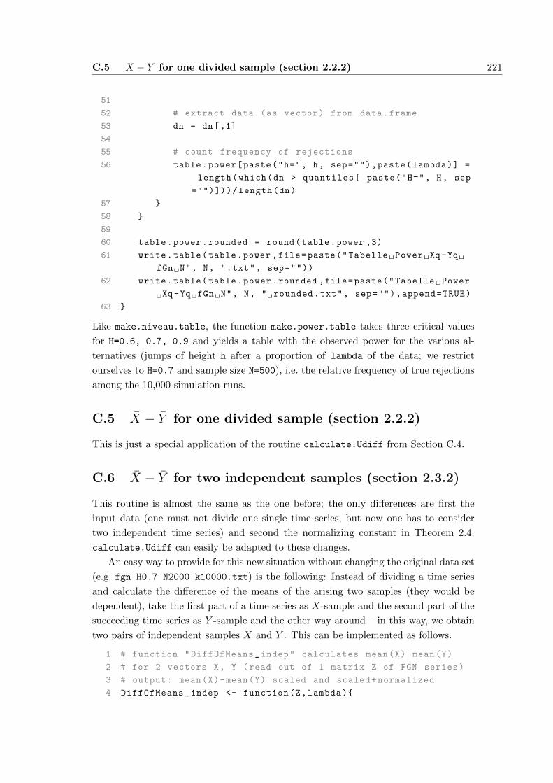
C.5 X − Y for one divided sample (section 2.2.2) 221
51
52 # extract data (as vector) from data.frame
53 dn = dn[,1]
54
55 # count frequency of rejections
56 table.power[paste("h=", h, sep=""),paste(lambda)] =
length(which(dn > quantiles[ paste("H=", H, sep
="")]))/length(dn)
57
58
59
60 table.power.rounded = round(table.power ,3)
61 write.table(table.power ,file=paste("Tabelle Power Xq -Yq
fGn N", N, ".txt", sep=""))
62 write.table(table.power.rounded ,file=paste("Tabelle Power
Xq-Yq fGn N", N, " rounded.txt", sep=""),append=TRUE)
63
Like make.niveau.table, the function make.power.table takes three critical values
for H=0.6, 0.7, 0.9 and yields a table with the observed power for the various al-
ternatives (jumps of height h after a proportion of lambda of the data; we restrict
ourselves to H=0.7 and sample size N=500), i.e. the relative frequency of true rejections
among the 10,000 simulation runs.
C.5 X − Y for one divided sample (section 2.2.2)
This is just a special application of the routine calculate.Udiff from Section C.4.
C.6 X − Y for two independent samples (section 2.3.2)
This routine is almost the same as the one before; the only differences are first the
input data (one must not divide one single time series, but now one has to consider
two independent time series) and second the normalizing constant in Theorem 2.4.
calculate.Udiff can easily be adapted to these changes.
An easy way to provide for this new situation without changing the original data set
(e.g. fgn H0.7 N2000 k10000.txt) is the following: Instead of dividing a time series
and calculate the difference of the means of the arising two samples (they would be
dependent), take the first part of a time series as X-sample and the second part of the
succeeding time series as Y -sample and the other way around – in this way, we obtain
two pairs of independent samples X and Y . This can be implemented as follows.
1 # function "DiffOfMeans_indep" calculates mean(X)-mean(Y)
2 # for 2 vectors X, Y (read out of 1 matrix Z of FGN series)
3 # output: mean(X)-mean(Y) scaled and scaled+normalized
4 DiffOfMeans_indep <- function(Z,lambda)
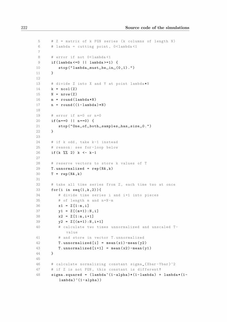
222 Source code of the simulations
5 # Z = matrix of k FGN series (k columns of length N)
6 # lambda = cutting point , 0<lambda <1
7
8 # error if not 0<lambda <1
9 if(lambda <=0 || lambda >=1)
10 stop("lambda must be in (0,1).")
11
12
13 # divide Z into X and Y at point lambda*N
14 k = ncol(Z)
15 N = nrow(Z)
16 m = round(lambda*N)
17 n = round((1- lambda)*N)
18
19 # error if m=0 or n=0
20 if(m==0 || n==0)
21 stop("One of both samples has size 0.")
22
23
24 # if k odd , take k-1 instead
25 # reason: see for -loop below
26 if(k %% 2) k <- k-1
27
28 # reserve vectors to store k values of T
29 T.unnormalized = rep(NA ,k)
30 T = rep(NA ,k)
31
32 # take all time series from Z, each time two at once
33 for(i in seq(1,k,2))
34 # divide time series i and i+1 into pieces
35 # of length m and n=N-m
36 x1 = Z[1:m,i]
37 y1 = Z[(m+1):N,i]
38 x2 = Z[1:m,i+1]
39 y2 = Z[(m+1):N,i+1]
40 # calculate two times unnormalized and unscaled T-
value
41 # and store in vector T.unnormalized
42 T.unnormalized[i] = mean(x1)-mean(y2)
43 T.unnormalized[i+1] = mean(x2)-mean(y1)
44
45
46 # calculate normalizing constant sigma_Xbar -Ybar ^2
47 # if Z is not FGN , this constant is different!
48 sigma.squared = (lambda ^(1- alpha)*(1-lambda) + lambda*(1-
lambda)^(1-alpha))

C.7 Quantiles of sup |Z(λ)− λZ(1)| (section 3.4) 223
49
50 # normalize and scale T.unnormalized
51 # to obtain limit distribution N(0,1) (predicted by
theory)
52 # if Z is not FGN , scaling is different!
53 T = T.unnormalized*sqrt(m*n/N^(2- alpha))/sqrt(sigma.
squared)
54
55 # scale T.unnormalized with overall sample size N (not
normalizing)
56 # if Z is not FGN , scaling is different!
57 T.unnormalized = T.unnormalized*N^( alpha/2)
58
59 write.table(T.unnormalized , file = paste("Xquer -Yquer N",
N, " lambda", lambda , " k", k, ".txt", sep = ""))
60 write.table(T, file = paste("Xquer -Yquer norm N", N, "
lambda", lambda , " k", k, ".txt", sep = ""))
61
C.7 Quantiles of sup |Z(λ)− λZ(1)| (section 3.4)
The distribution of sup0≤λ≤1 |Z(λ) − λZ(1)| was simulated, as described on page 61,
with the following code.
1 simulate.distribution.Dn <- function(H)
2 # fArma: long -range dependend time series
3 library(fArma)
4
5 alpha = 2-2*H
6
7 # from 0 to 1 in steps
8 # k repetitions
9 steps = seq (0 ,1 ,0.001)
10 l = length(steps)
11 k = 10000
12
13 # reserve vector Z for time series Z at l times
14 # reserve vectors for simulation result
15 Z = rep(NA ,l)
16 result.different.lambdas = rep(NA ,l)
17 result = rep(NA ,k)
18
19 # j=1,...,k (repetitions)
20 for(j in 1:k)
21 # simulate fBm with time in [0,1] at l equidistant
points 0, ..., 1

224 Source code of the simulations
22 Z = fbmSim(l, H, doplot=F);
23
24 # for each time lambda =0,...,1
25 i = 1
26 for(lambda in steps)
27 # calculate Z(lambda)-lambda Z(lambda)
28 # remember that Z is a vector with entries Z[1], Z
[2], ...
29 lambda2 = lambda*(l-1)+1
30 result.different.lambdas[i] = Z[lambda2]-lambda*Z[l
]
31 i=i+1
32
33
34 # store the max of the absolute value to obtain 1
realization
35 result[j] = max(abs(result.different.lambdas))
36
37
38 write.table(result , file = paste("Xquer -Yquer Vtlg CP -
test fGn H=", H, " steps=", l, ".txt", sep = ""))
39
40 detach("package:fArma")
41
The routine simulate.distribution.Dn produces a file, e.g. Xquer-Yquer Vtlg CP-test
fGn H=.7 steps=1001.txt, with 10000 simulation results of sup0≤λ≤1 |Z(λ)− λZ(1)|from which properties like the quantiles of the distribution of sup0≤λ≤1 |Z(λ)− λZ(1)|can be approximated.
C.8 “Wilcoxon-type” test (section 3.6)
The following program code calculates k repetitions of the “Wilcox-type” test statistic
Wn, as defined in (3.12) for different sample lengths N and LRD parameter H. The input
needed, the design of the routine (for fGn; it must be adapted if th underlying Gaussian
process is not fGn), the workflow needed and the output is like for the “diferences-of-
means” test in section C.4.
1 # function divides vector vec after entry with index cut
2 # and gives Wilcoxon statistic
3 divide.and.Wilcox <- function(vec , cut)
4 l = length(vec)
5
6 # function counts , how many entries of vector vv are >= n
7 which.vv.greater.n <- function(n,vv) length(which(n<=vv))
8

C.8 “Wilcoxon-type” test (section 3.6) 225
9 # function compares all entries of a vector vec1
10 # with a vector vec2 via "which.vv.greater.n"
11 which.vec1.smaller.vec2 <- function(vec1 , vec2) sum(
sapply(vec1 , which.vv.greater.n, vv=vec2))
12
13 # finally apply "which.vec1.smaller.vec2" to
14 # first and second part of vec
15 which.vec1.smaller.vec2(vec [1: cut], vec[(cut +1):l])
16
17
18 # function calculates
19 # U_W = 1/(n dn) sum_i=1^ lambda n sum_j=lambda n+1^n (
I(Xi <=Xj - 1/2)
20 # for two vectors X, Y (created by dividing one FGN series Z
)
21 # returns vector with 10.000 values of U_W
22 calculate.U_W <- function(Z, cutpt , alpha)
23 # Z = given matrix of k FGN series (k columns of length N
)
24 # cutting point cutpt= 1,...,N-1
25
26 # error if cutting point not an integer number
27 if(cutpt - trunc(cutpt) != 0)
28 stop("cutpoint is not an integer.")
29
30
31 # read dimensions of Z
32 k = ncol(Z)
33 N = nrow(Z)
34
35 # reserve vector U to store k values of U_W
36 U = rep(NA ,k)
37
38 # cutting point should be in 1,2, ..., N-1
39 if(( cutpt >= 1) && (cutpt < N))
40 # apply "divide.and.difference" to columns of Z
41 # and write k results in vector U
42 U = apply(Z, 2, divide.and.Wilcox , cut=cutpt)
43
44
45 # if cutpt out of range , T can ’t be calculated
46 if(( cutpt < 1) || (cutpt >= N))
47 U = rep(NA ,k)
48
49
50 lambd = cutpt/N
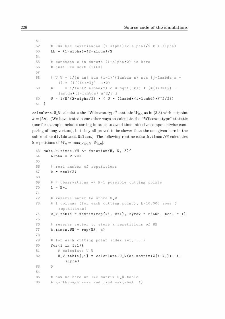
226 Source code of the simulations
51
52 # FGN has covariances (1-alpha)(2-alpha)/2 k^(-alpha)
53 Lk = (1-alpha)*(2-alpha)/2
54
55 # constant c in dn=c*n^(1- alpha/2) is here
56 # just: c= sqrt (1/Lk)
57
58 # U_W = 1/(n dn) sum_i=1^ lambda n sum_j=lambda n +
1^n (I(Xi <=Xj -1/2)
59 # = 1/(n^(2- alpha/2) c * sqrt(Lk)) * [#Xi <=Xj -
lambda*(1-lambda) n^2/2 ]
60 U = 1/N^(2- alpha/2) * ( U - (lambd*(1-lambd)*N^2/2))
61
calculate.U_W calculates the “Wilcoxon-type” statistic Wk,n as in (3.3) with cutpoint
k = [λn]. (We have tested some other ways to calculate the “Wilcoxon-type” statistic
(one for example includes sorting in order to avoid time intensive componentwise com-
paring of long vectors), but they all proved to be slower than the one given here in the
sub-routine divide.and.Wilcox.) The following routine make.k.times.WN calculates
k repetitions of Wn = max1≤k<N |Wk,n|.
63 make.k.times.WN <- function(H, N, Z)
64 alpha = 2-2*H
65
66 # read number of repetitions
67 k = ncol(Z)
68
69 # N observations => N-1 possible cutting points
70 l = N-1
71
72 # reserve marix to store U_W
73 # l columns (for each cutting point), k=10.000 rows (
repetitions)
74 U_W.table = matrix(rep(NA , k*l), byrow = FALSE , ncol = l)
75
76 # reserve vector to store k repetitions of WN
77 k.times.WN = rep(NA , k)
78
79 # for each cutting point index i=1,...,N
80 for(i in 1:l)
81 # calculate U_W
82 U_W.table[,i] = calculate.U_W(as.matrix(Z[1:N,]), i,
alpha)
83
84
85 # now we have an lxk matrix U_W.table
86 # go through rows and find max(abs (..))
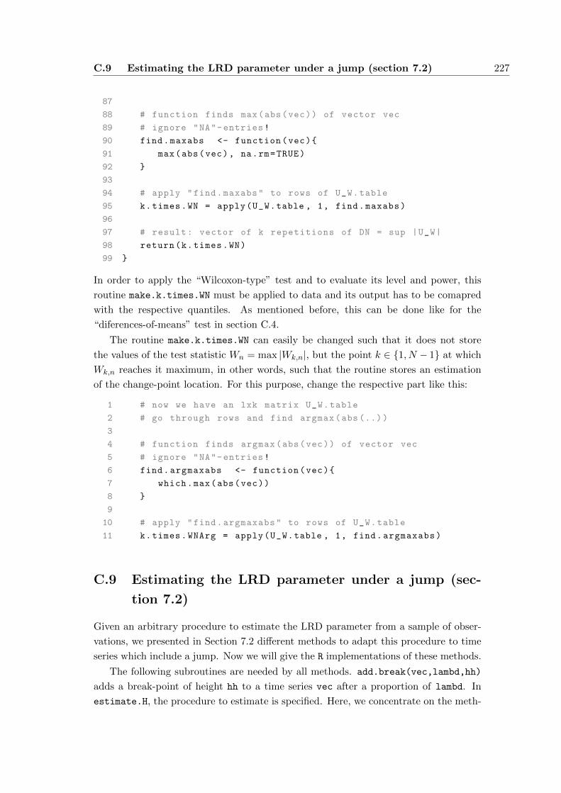
C.9 Estimating the LRD parameter under a jump (section 7.2) 227
87
88 # function finds max(abs(vec)) of vector vec
89 # ignore "NA"-entries!
90 find.maxabs <- function(vec)
91 max(abs(vec), na.rm=TRUE)
92
93
94 # apply "find.maxabs" to rows of U_W.table
95 k.times.WN = apply(U_W.table , 1, find.maxabs)
96
97 # result: vector of k repetitions of DN = sup |U_W|
98 return(k.times.WN)
99
In order to apply the “Wilcoxon-type” test and to evaluate its level and power, this
routine make.k.times.WN must be applied to data and its output has to be comapred
with the respective quantiles. As mentioned before, this can be done like for the
“diferences-of-means” test in section C.4.
The routine make.k.times.WN can easily be changed such that it does not store
the values of the test statistic Wn = max |Wk,n|, but the point k ∈ 1, N − 1 at which
Wk,n reaches it maximum, in other words, such that the routine stores an estimation
of the change-point location. For this purpose, change the respective part like this:
1 # now we have an lxk matrix U_W.table
2 # go through rows and find argmax(abs (..))
3
4 # function finds argmax(abs(vec)) of vector vec
5 # ignore "NA"-entries!
6 find.argmaxabs <- function(vec)
7 which.max(abs(vec))
8
9
10 # apply "find.argmaxabs" to rows of U_W.table
11 k.times.WNArg = apply(U_W.table , 1, find.argmaxabs)
C.9 Estimating the LRD parameter under a jump (sec-
tion 7.2)
Given an arbitrary procedure to estimate the LRD parameter from a sample of obser-
vations, we presented in Section 7.2 different methods to adapt this procedure to time
series which include a jump. Now we will give the R implementations of these methods.
The following subroutines are needed by all methods. add.break(vec,lambd,hh)
adds a break-point of height hh to a time series vec after a proportion of lambd. In
estimate.H, the procedure to estimate is specified. Here, we concentrate on the meth-

228 Source code of the simulations
ods whittleFit and boxperFit from the fArma package. The routine estimate.H.try
handles errors: If estimate.H produces an error, it gives out NA.
1 add.break <- function(vec , lambd , hh)
2 ll = length(vec)
3 m = floor(lambd*ll)
4 vec.neu = c(vec [1:m], vec[(m+1):ll] + hh)
5 vec.neu
6
7
8 estimate.H <- function(vec)
9 library(fArma)
10 #y = whittleFit(vec)
11 #y@hurst [[3]]
12 y = boxperFit(vec)
13 y@hurst [[1]]
14
15
16 estimate.H.try <- function(vec)
17 return(tryCatch(
18 estimate.H(vec),
19 error=function(e) NA
20 ))
21
With the following routines, the LRD parameter is estimated on each two blocks
which arise from cutting the sample in two pieces. This is done for all cutting points
(leaving out the margins of the sample). The third routine then calculates a function
of these pairs of estimates – the means of all estimates or the mean of the two estimates
at the cutting point where both estimates (left and right block) differ least.
1 # estimate H seperately on index set
2 # I1=1,...,k and I2 = k+1, ..., n
3 estimate.H.piecewise <- function(vec , cutpoint)
4 N = length(vec)
5 H.lower = estimate.H.try(vec [1: cutpoint ])
6 H.upper = estimate.H.try(vec[( cutpoint +1):N])
7 c(H.lower , H.upper)
8
9
10 calculate.all.Hpiecewise <- function(vec)
11 N = length(vec)
12 lower = max(c(floor(N*0.10), 10))+1
13 upper = N-lower
14 Hpiecewise = matrix(rep(NA , 2*(upper -lower +1)), ncol =2)
15 for(i in lower:upper)
16 Hpiecewise[i-lower+1,] = estimate.H.piecewise(vec , i)
17

C.9 Estimating the LRD parameter under a jump (section 7.2) 229
18 Hpiecewise
19
20
21 estimate.H.block <- function(vec)
22 Hpiecewise = calculate.all.Hpiecewise(vec)
23 RMeans = rowMeans(Hpiecewise , na.rm=TRUE)
24
25 H.mean = mean(RMeans , na.rm=TRUE)
26 H.mindiff = mean(estimate.H.piecewise(vec , which.min(abs(
Hpiecewise [,2]- Hpiecewise [,1]))))
27 c(H.mean , H.mindiff)
28
Now we give the code for estimating H on a moving (overlapping) window with
flank size w (i.e. a windowf of size 2w+1) from the data vec.
1 estimate.H.movwin <- function(vec , w)
2 N = length(vec)
3
4 window.indices <- function(w, midpoint)
5 # w = half window size
6 # if midpoint <= w, some indices <= 0, fill with "NA"
7 # should not happen , but to be on the safe side :-)
8 if(midpoint > w) indices = seq(midpoint -w, midpoint+w)
9 if(midpoint <= w)
10 indices = seq(midpoint -w, midpoint+w)
11 indices[which(indices <=0)] = NA
12
13 indices
14
15
16 window.midpoints = seq(w+1, N-w)
17 H.movwin = rep(NA , length(window.midpoints))
18
19 # move index window [x-w, x+w] from x=w+1 to x=N-w
20 for(i in window.midpoints)
21 H.movwin[i] = estimate.H.try(vec[window.indices(w, i)
])
22
23 mean(H.movwin , na.rm=TRUE)
24
And this the code for a non-overlapping moving window based estimation:
26 estimate.H.movwin.nonlap <- function(vec , w)
27 N = length(vec)
28 # w: window size
29
30 window.startpoints = seq(1, N, w)

230 Source code of the simulations
31 # remove last startpoint , if last window smaller than w
32 if(N%%w!=0)
33 window.startpoints = window.startpoints[-length(window
.startpoints)]
34
35
36 H.movwin.nonlap = rep(NA , length(window.startpoints))
37
38 counter = 1
39 for(i in window.startpoints)
40 H.movwin.nonlap[counter] = estimate.H.try(vec[i:(i+w
-1)])
41 counter=counter +1
42
43 mean(H.movwin.nonlap , na.rm=TRUE)
44
In what follows, we present the code for estimating H using pre-estimation of
the possible change-point. This approach needs a method to estimate the change-
point location, here this is the routine make.k.times.WNArg, a simple modification of
make.k.times.WN as defined above at the end of Section C.8.
45 estimate.H.preestimate <- function(vec)
46 N = length(vec)
47
48 # load Wilcoxon change -point test statistic
49
50 # estimate H seperately on index set
51 # I1=1,...,k and I2 = k+1, ..., n
52 estimate.H.piecewise <- function(vec , cutpoint)
53 N = length(vec)
54 H.lower = estimate.H.try(vec [1: cutpoint ])
55 H.upper = estimate.H.try(vec[( cutpoint +1):N])
56 c(H.lower , H.upper)
57
58
59 # start with arbitrary value for H, e.g. usual estimate
60 H.estim.usual = estimate.H.try(vec)
61
62 # under H=H.estim.usual , where detects Wilcoxon test
change -point?
63 CP.estim = make.k.times.WNArg(H.estim.usual , N, as.matrix
(vec))
64
65 # way 1:
66 # estimate H on block before and after this change -point
67 H.estim.2 blocks = estimate.H.piecewise(vec , CP.estim)

C.9 Estimating the LRD parameter under a jump (section 7.2) 231
68 H.estim.2 blocks = mean(H.estim.2 blocks)
69 # assign new estimate to H? No. Because:
70 # from now on , cp -detection will not change ,
71 # since H changes only scaling
72 # => new H maybe changes test decision , but not argmax
73
74 # way 2:
75 # remove jump and estimate H on whole time series
76 remove.jump <- function(vec)
77 N = length(vec)
78 # under H=H.estim.usual , where detects Wilcoxon test
change -point?
79 H.estim.usual = estimate.H.try(vec)
80 CP.estim = make.k.times.WNArg(H.estim.usual , N, as.
matrix(vec))
81
82 # if H.estim.usual returns NA , CP.estim = integer (0),
i.e.\ length 0 vector
83 if(length(CP.estim)!=0)
84 # estimate jump height
85 h.estim = mean(vec[(CP.estim +1):N])-mean(vec [1:CP.
estim])
86 # remove jump
87 vec.jumpfree = c(vec [1:CP.estim], vec[(CP.estim +1):
N]-h.estim)
88 else
89 vec.jumpfree = NA
90
91 vec.jumpfree
92
93
94 # estimate H on whole time series without jump
95 vec.jumpfree = remove.jump(vec)
96 H.estim.jumpfree = estimate.H.try(vec.jumpfree)
97
98 # way 3:
99 # repeat way 2 iteratively
100 # drawback: many repetitions smoothe time series=> H
underestimated
101 estimate.jumpfree.iterative <- function(vect)
102 # set start values
103 H.iterativ = 2
104 H.Differenz = 2
105 counter = 0
106 while(abs(H.Differenz) > 0.01)
107 # remove jump from vec

232 Source code of the simulations
108 vect.jumpfree = remove.jump(vect)
109 # estimate H on time series without jump
110 H.estim.jumpfree = estimate.H.try(vect.jumpfree)
111
112 # did H.estim.jumpfree change?
113 H.Differenz = H.iterativ -H.estim.jumpfree
114 # if yes , try another run , based on jumpfree series
115 vect = vect.jumpfree
116 H.iterativ = H.estim.jumpfree
117 counter = counter + 1
118
119 c(H.iterativ , counter)
120
121 # estimate.jumpfree.iterative(vec)
122
123 c(H.estim.jumpfree , H.estim.2 blocks)
124
C.10 Estimating the first Hermite coefficient (section 7.3)
The program simulateCoeff1 produces a table in which the estimations a1 for a1, as
defined in (7.3), are given – each the mean and the variance in 10,000 simulation runs
for different sample sizes. For a better comparison, the mean is given relative to the
true value a1; if this value is not known, the program must be adapted.
1 simulateCoeff1 <- function(G, decreas=FALSE , trueCoef , zv.
lrd=FALSE)
2 # G: function G that generates data
3 # decreas: Is G decreasing?
4 # trueCoef: true first Hermite coefficient of G
5 # zv.lrd: replace true xi by new xi iid or lrd
6
7 library(fArma)
8 H = 0.7
9 alpha = 2-2*H
10
11 simCoeff.norm.sort <- function(n, G, decreas , H)
12 # replace true xi by new xi\sim N(0,1) iid
13 xi = rnorm(n)
14 x = G(fgnSim(n, H))
15 mean(sort(xi)*sort(x, decreasing=decreas))
16
17
18 simCoeff.LRD.sort <- function(n, G, decreas , H)
19 # replace true xi by new xi\sim N(0,1) LRD
20 xi = fgnSim(n, H)

C.10 Estimating the first Hermite coefficient (section 7.3) 233
21 x = G(fgnSim(n, H))
22 mean(sort(xi)*sort(x, decreasing=decreas))
23
24
25 # k = number of repititions
26 k = 10000
27 Tnorm = rep(NA , k)
28
29 NN = c(10, 50, 100, 500, 1000, 2000, 5000, 10000)
30
31 Results = matrix(rep(NA ,length(NN)*2), byrow = FALSE ,
ncol = 2)
32 colnames(Results) = c(’mean/true’, ’variance ’)
33 rownames(Results) = NN
34
35 for(n in NN)
36 for(i in 1:k)
37 Tnorm[i] = if(zv.lrd) simCoeff.LRD.sort(n, G,
decreas , H) else simCoeff.norm.sort(n, G,
decreas , H)
38
39 Results[paste(n) ,1] = mean(Tnorm)
40 Results[paste(n) ,2] = var(Tnorm)
41
42
43 Results [,1] = Results [,1]/trueCoef
44
45 Results
46

234 Source code of the simulations
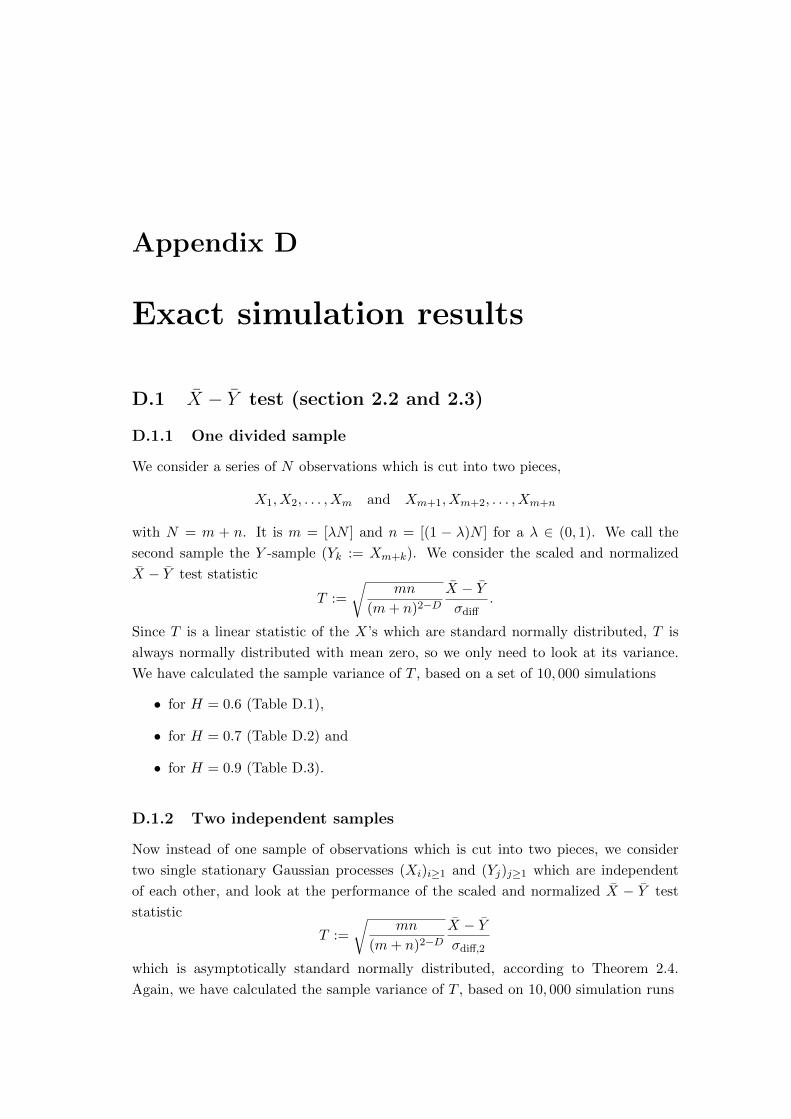
Appendix D
Exact simulation results
D.1 X − Y test (section 2.2 and 2.3)
D.1.1 One divided sample
We consider a series of N observations which is cut into two pieces,
X1, X2, . . . , Xm and Xm+1, Xm+2, . . . , Xm+n
with N = m + n. It is m = [λN ] and n = [(1 − λ)N ] for a λ ∈ (0, 1). We call the
second sample the Y -sample (Yk := Xm+k). We consider the scaled and normalized
X − Y test statistic
T :=
√mn
(m+ n)2−DX − Yσdiff
.
Since T is a linear statistic of the X’s which are standard normally distributed, T is
always normally distributed with mean zero, so we only need to look at its variance.
We have calculated the sample variance of T , based on a set of 10, 000 simulations
• for H = 0.6 (Table D.1),
• for H = 0.7 (Table D.2) and
• for H = 0.9 (Table D.3).
D.1.2 Two independent samples
Now instead of one sample of observations which is cut into two pieces, we consider
two single stationary Gaussian processes (Xi)i≥1 and (Yj)j≥1 which are independent
of each other, and look at the performance of the scaled and normalized X − Y test
statistic
T :=
√mn
(m+ n)2−DX − Yσdiff,2
which is asymptotically standard normally distributed, according to Theorem 2.4.
Again, we have calculated the sample variance of T , based on 10, 000 simulation runs

236 Exact simulation results
N \ λ 0.1 0.2 0.3 0.4 0.5 0.6 0.7 0.8 0.9
10 0.98 0.989 1.014 1.026 1.028 1.004 1.005 1.004 0.983
50 0.999 0.962 0.963 0.971 0.989 0.994 0.997 1.011 0.998
100 0.963 0.98 0.996 0.997 0.992 0.981 0.978 0.982 0.995
500 0.977 0.985 1.003 1.008 1.03 1.014 1.002 0.999 0.997
1000 1.004 1.016 1.013 1.004 0.996 1.002 1.009 0.991 0.986
2000 1.008 0.997 0.989 0.985 0.992 0.986 0.982 0.982 0.995
Table D.1: Sample variance of 10, 000 values of T for fGn with Hurst parameter H = 0.6
(D = 0.8). N is the overall sample size, the data was divided into two samples after
the [λN ]-th observation.
N \ λ 0.1 0.2 0.3 0.4 0.5 0.6 0.7 0.8 0.9
10 0.992 0.993 0.992 0.997 1.003 1.007 1.007 1.001 1.002
50 1.023 1.015 0.996 0.989 0.995 0.994 0.986 1.003 0.992
100 1.025 1.006 1 1.014 1.008 1.008 0.997 0.989 0.992
500 1.001 0.984 0.994 0.997 0.992 0.993 0.994 0.985 0.991
1000 0.984 1.004 1.014 1.015 1.017 1.004 1.005 1.008 1.008
2000 1.003 1.005 0.998 1.002 0.992 1 1.011 1.014 1.02
Table D.2: Sample variance of 10, 000 values of T for fGn with Hurst parameter H = 0.7
(D = 0.6). N is the overall sample size, the data was divided into two samples after
the [λN ]-th observation.
N \ λ 0.1 0.2 0.3 0.4 0.5 0.6 0.7 0.8 0.9
10 0.988 0.995 1.001 1.014 1.007 1.012 1.003 0.99 1.005
50 1 0.995 0.997 0.992 0.99 0.999 1.001 1.007 1.012
100 1.002 0.996 0.996 0.995 0.991 0.997 1.007 1.008 1.012
500 1 0.996 0.985 0.986 0.981 0.99 0.991 0.993 0.997
1000 0.999 0.99 1.001 1.007 1.011 1.02 1.011 0.998 1
2000 0.99 1.003 1.011 1.004 1.007 0.998 1.003 1.011 0.999
Table D.3: Sample variance of 10, 000 values of T for fGn with Hurst parameter H = 0.9
(D = 0.2). N is the overall sample size, the data was divided into two samples after
the [λN ]-th observation.

D.1 X − Y test (section 2.2 and 2.3) 237
• for H = 0.6 (Table D.4),
• for H = 0.7 (Table D.5) and
• for H = 0.9 (Table D.6).
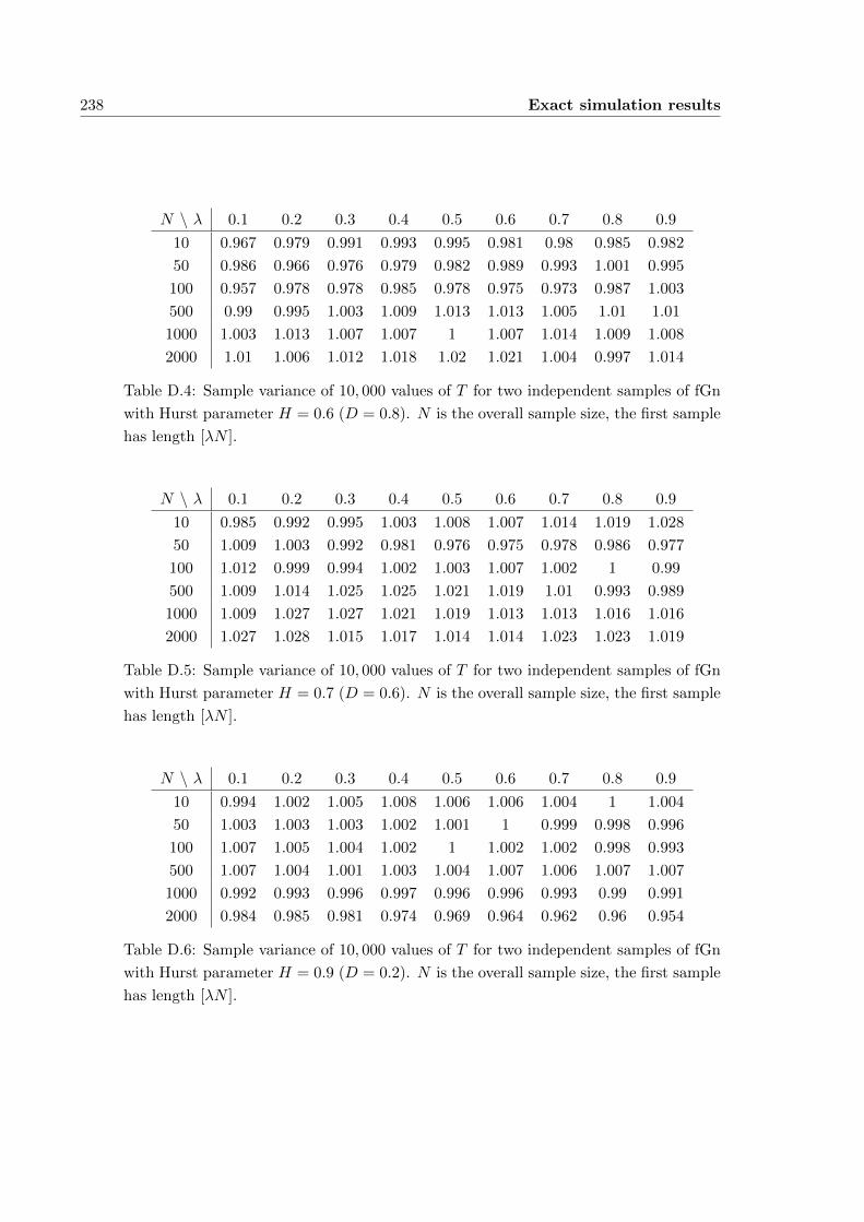
238 Exact simulation results
N \ λ 0.1 0.2 0.3 0.4 0.5 0.6 0.7 0.8 0.9
10 0.967 0.979 0.991 0.993 0.995 0.981 0.98 0.985 0.982
50 0.986 0.966 0.976 0.979 0.982 0.989 0.993 1.001 0.995
100 0.957 0.978 0.978 0.985 0.978 0.975 0.973 0.987 1.003
500 0.99 0.995 1.003 1.009 1.013 1.013 1.005 1.01 1.01
1000 1.003 1.013 1.007 1.007 1 1.007 1.014 1.009 1.008
2000 1.01 1.006 1.012 1.018 1.02 1.021 1.004 0.997 1.014
Table D.4: Sample variance of 10, 000 values of T for two independent samples of fGn
with Hurst parameter H = 0.6 (D = 0.8). N is the overall sample size, the first sample
has length [λN ].
N \ λ 0.1 0.2 0.3 0.4 0.5 0.6 0.7 0.8 0.9
10 0.985 0.992 0.995 1.003 1.008 1.007 1.014 1.019 1.028
50 1.009 1.003 0.992 0.981 0.976 0.975 0.978 0.986 0.977
100 1.012 0.999 0.994 1.002 1.003 1.007 1.002 1 0.99
500 1.009 1.014 1.025 1.025 1.021 1.019 1.01 0.993 0.989
1000 1.009 1.027 1.027 1.021 1.019 1.013 1.013 1.016 1.016
2000 1.027 1.028 1.015 1.017 1.014 1.014 1.023 1.023 1.019
Table D.5: Sample variance of 10, 000 values of T for two independent samples of fGn
with Hurst parameter H = 0.7 (D = 0.6). N is the overall sample size, the first sample
has length [λN ].
N \ λ 0.1 0.2 0.3 0.4 0.5 0.6 0.7 0.8 0.9
10 0.994 1.002 1.005 1.008 1.006 1.006 1.004 1 1.004
50 1.003 1.003 1.003 1.002 1.001 1 0.999 0.998 0.996
100 1.007 1.005 1.004 1.002 1 1.002 1.002 0.998 0.993
500 1.007 1.004 1.001 1.003 1.004 1.007 1.006 1.007 1.007
1000 0.992 0.993 0.996 0.997 0.996 0.996 0.993 0.99 0.991
2000 0.984 0.985 0.981 0.974 0.969 0.964 0.962 0.96 0.954
Table D.6: Sample variance of 10, 000 values of T for two independent samples of fGn
with Hurst parameter H = 0.9 (D = 0.2). N is the overall sample size, the first sample
has length [λN ].
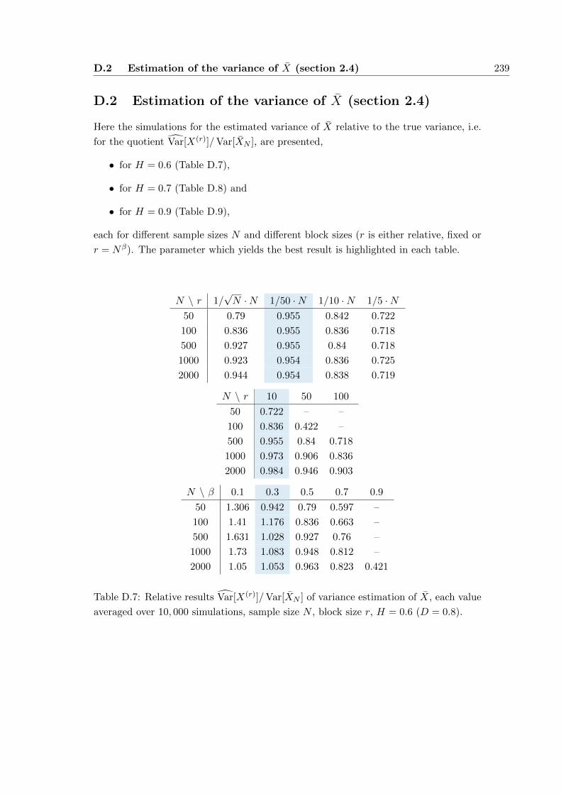
D.2 Estimation of the variance of X (section 2.4) 239
D.2 Estimation of the variance of X (section 2.4)
Here the simulations for the estimated variance of X relative to the true variance, i.e.
for the quotient Var[X(r)]/Var[XN ], are presented,
• for H = 0.6 (Table D.7),
• for H = 0.7 (Table D.8) and
• for H = 0.9 (Table D.9),
each for different sample sizes N and different block sizes (r is either relative, fixed or
r = Nβ). The parameter which yields the best result is highlighted in each table.
N \ r 1/√N ·N 1/50 ·N 1/10 ·N 1/5 ·N
50 0.79 0.955 0.842 0.722
100 0.836 0.955 0.836 0.718
500 0.927 0.955 0.84 0.718
1000 0.923 0.954 0.836 0.725
2000 0.944 0.954 0.838 0.719
N \ r 10 50 100
50 0.722 – –
100 0.836 0.422 –
500 0.955 0.84 0.718
1000 0.973 0.906 0.836
2000 0.984 0.946 0.903
N \ β 0.1 0.3 0.5 0.7 0.9
50 1.306 0.942 0.79 0.597 –
100 1.41 1.176 0.836 0.663 –
500 1.631 1.028 0.927 0.76 –
1000 1.73 1.083 0.948 0.812 –
2000 1.05 1.053 0.963 0.823 0.421
Table D.7: Relative results Var[X(r)]/Var[XN ] of variance estimation of X, each value
averaged over 10, 000 simulations, sample size N , block size r, H = 0.6 (D = 0.8).
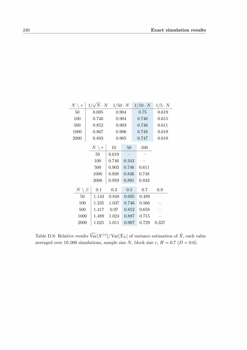
240 Exact simulation results
N \ r 1/√N ·N 1/50 ·N 1/10 ·N 1/5 ·N
50 0.695 0.904 0.75 0.619
100 0.746 0.904 0.746 0.615
500 0.852 0.903 0.746 0.611
1000 0.867 0.906 0.748 0.619
2000 0.893 0.905 0.747 0.619
N \ r 10 50 100
50 0.619 – –
100 0.746 0.343 –
500 0.903 0.746 0.611
1000 0.938 0.836 0.748
2000 0.959 0.891 0.833
N \ β 0.1 0.3 0.5 0.7 0.9
50 1.143 0.848 0.695 0.489 –
100 1.235 1.037 0.746 0.566 –
500 1.417 0.97 0.852 0.658 –
1000 1.489 1.024 0.887 0.715 –
2000 1.025 1.011 0.907 0.729 0.337
Table D.8: Relative results Var[X(r)]/Var[XN ] of variance estimation of X, each value
averaged over 10, 000 simulations, sample size N , block size r, H = 0.7 (D = 0.6).
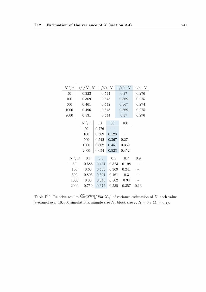
D.2 Estimation of the variance of X (section 2.4) 241
N \ r 1/√N ·N 1/50 ·N 1/10 ·N 1/5 ·N
50 0.323 0.544 0.37 0.276
100 0.369 0.543 0.369 0.275
500 0.461 0.542 0.367 0.274
1000 0.496 0.543 0.369 0.275
2000 0.531 0.544 0.37 0.276
N \ r 10 50 100
50 0.276 – –
100 0.369 0.128 –
500 0.542 0.367 0.274
1000 0.602 0.451 0.369
2000 0.654 0.523 0.452
N \ β 0.1 0.3 0.5 0.7 0.9
50 0.588 0.434 0.323 0.198 –
100 0.66 0.533 0.369 0.241 –
500 0.805 0.594 0.461 0.3 –
1000 0.86 0.645 0.502 0.34 –
2000 0.759 0.672 0.535 0.357 0.13
Table D.9: Relative results Var[X(r)]/Var[XN ] of variance estimation of X, each value
averaged over 10, 000 simulations, sample size N , block size r, H = 0.9 (D = 0.2).
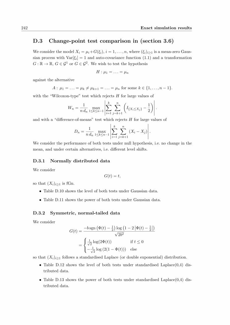
242 Exact simulation results
D.3 Change-point test comparison in (section 3.6)
We consider the model Xi = µi+G(ξi), i = 1, . . . , n, where (ξi)i≥1 is a mean-zero Gaus-
sian process with Var[ξi] = 1 and auto-covariance function (1.1) and a transformation
G : R→ R, G ∈ G1 or G ∈ G2. We wish to test the hypothesis
H : µ1 = . . . = µn
against the alternative
A : µ1 = . . . = µk 6= µk+1 = . . . = µn for some k ∈ 1, . . . , n− 1.
with the “Wilcoxon-type” test which rejects H for large values of
Wn =1
ndnmax
1≤k≤n−1
∣∣∣∣∣∣k∑i=1
n∑j=k+1
(IXi≤Xj −
1
2
)∣∣∣∣∣∣ .and with a “difference-of-means” test which rejects H for large values of
Dn =1
ndnmax
1≤k≤n−1
∣∣∣∣∣∣k∑i=1
n∑j=k+1
(Xi −Xj)
∣∣∣∣∣∣ .We consider the performance of both tests under null hypothesis, i.e. no change in the
mean, and under certain alternatives, i.e. different level shifts.
D.3.1 Normally distributed data
We consider
G(t) = t,
so that (Xi)i≥1 is fGn.
• Table D.10 shows the level of both tests under Gaussian data.
• Table D.11 shows the power of both tests under Gaussian data.
D.3.2 Symmetric, normal-tailed data
We consider
G(t) =−b sgn
(Φ(t)− 1
2
)log(1− 2
∣∣Φ(t)− 12
∣∣)√
2b2
=
1√2
log(2Φ(t)) if t ≤ 0
− 1√2
log (2(1− Φ(t))) else
so that (Xi)i≥1 follows a standardised Laplace (or double exponential) distribution.
• Table D.12 shows the level of both tests under standardised Laplace(0,4) dis-
tributed data.
• Table D.13 shows the power of both tests under standardised Laplace(0,4) dis-
tributed data.
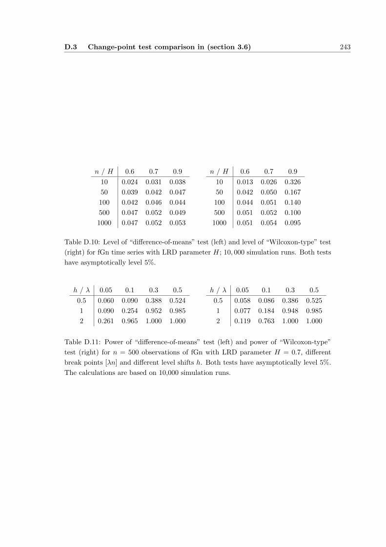
D.3 Change-point test comparison in (section 3.6) 243
n / H 0.6 0.7 0.9
10 0.024 0.031 0.038
50 0.039 0.042 0.047
100 0.042 0.046 0.044
500 0.047 0.052 0.049
1000 0.047 0.052 0.053
n / H 0.6 0.7 0.9
10 0.013 0.026 0.326
50 0.042 0.050 0.167
100 0.044 0.051 0.140
500 0.051 0.052 0.100
1000 0.051 0.054 0.095
Table D.10: Level of “difference-of-means” test (left) and level of “Wilcoxon-type” test
(right) for fGn time series with LRD parameter H; 10, 000 simulation runs. Both tests
have asymptotically level 5%.
h / λ 0.05 0.1 0.3 0.5
0.5 0.060 0.090 0.388 0.524
1 0.090 0.254 0.952 0.985
2 0.261 0.965 1.000 1.000
h / λ 0.05 0.1 0.3 0.5
0.5 0.058 0.086 0.386 0.525
1 0.077 0.184 0.948 0.985
2 0.119 0.763 1.000 1.000
Table D.11: Power of “difference-of-means” test (left) and power of “Wilcoxon-type”
test (right) for n = 500 observations of fGn with LRD parameter H = 0.7, different
break points [λn] and different level shifts h. Both tests have asymptotically level 5%.
The calculations are based on 10,000 simulation runs.
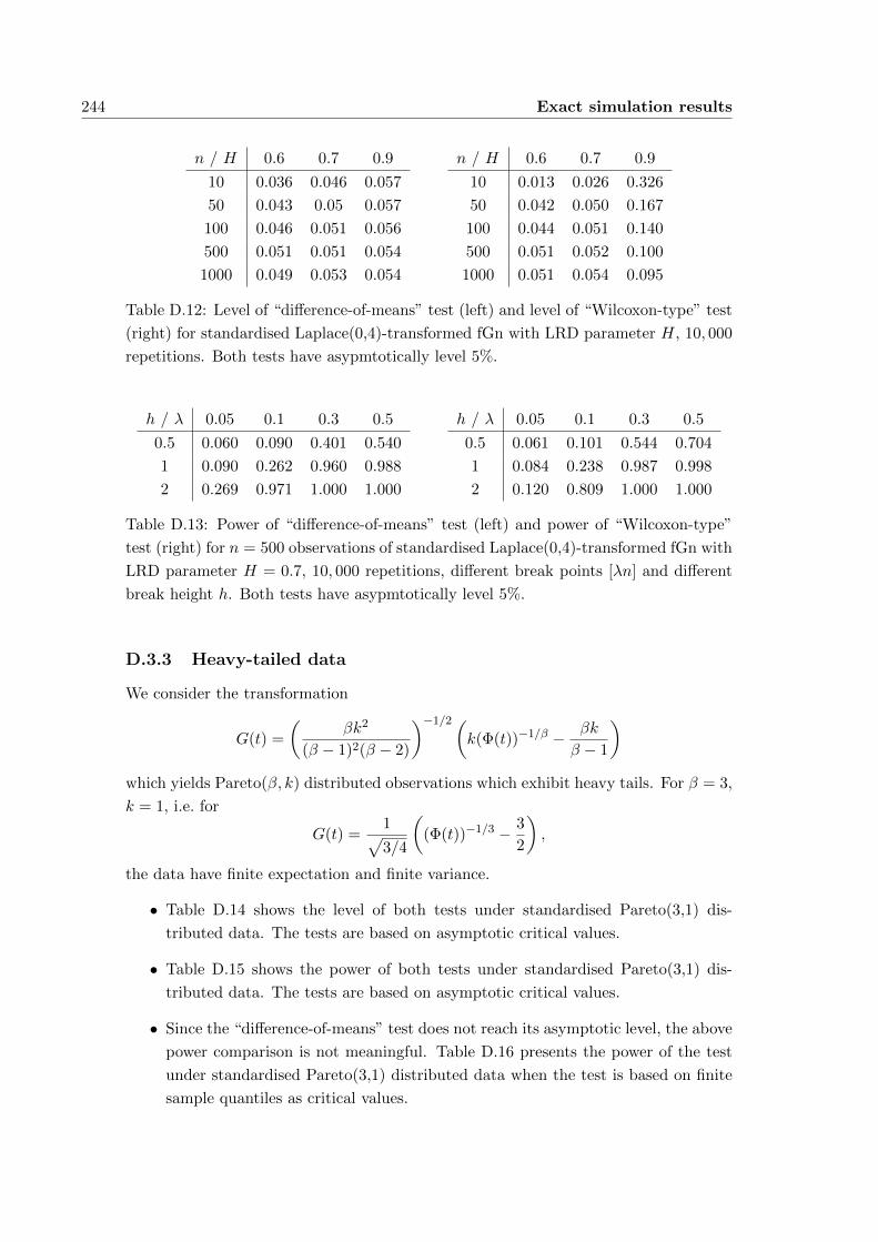
244 Exact simulation results
n / H 0.6 0.7 0.9
10 0.036 0.046 0.057
50 0.043 0.05 0.057
100 0.046 0.051 0.056
500 0.051 0.051 0.054
1000 0.049 0.053 0.054
n / H 0.6 0.7 0.9
10 0.013 0.026 0.326
50 0.042 0.050 0.167
100 0.044 0.051 0.140
500 0.051 0.052 0.100
1000 0.051 0.054 0.095
Table D.12: Level of “difference-of-means” test (left) and level of “Wilcoxon-type” test
(right) for standardised Laplace(0,4)-transformed fGn with LRD parameter H, 10, 000
repetitions. Both tests have asypmtotically level 5%.
h / λ 0.05 0.1 0.3 0.5
0.5 0.060 0.090 0.401 0.540
1 0.090 0.262 0.960 0.988
2 0.269 0.971 1.000 1.000
h / λ 0.05 0.1 0.3 0.5
0.5 0.061 0.101 0.544 0.704
1 0.084 0.238 0.987 0.998
2 0.120 0.809 1.000 1.000
Table D.13: Power of “difference-of-means” test (left) and power of “Wilcoxon-type”
test (right) for n = 500 observations of standardised Laplace(0,4)-transformed fGn with
LRD parameter H = 0.7, 10, 000 repetitions, different break points [λn] and different
break height h. Both tests have asypmtotically level 5%.
D.3.3 Heavy-tailed data
We consider the transformation
G(t) =
(βk2
(β − 1)2(β − 2)
)−1/2(k(Φ(t))−1/β − βk
β − 1
)which yields Pareto(β, k) distributed observations which exhibit heavy tails. For β = 3,
k = 1, i.e. for
G(t) =1√3/4
((Φ(t))−1/3 − 3
2
),
the data have finite expectation and finite variance.
• Table D.14 shows the level of both tests under standardised Pareto(3,1) dis-
tributed data. The tests are based on asymptotic critical values.
• Table D.15 shows the power of both tests under standardised Pareto(3,1) dis-
tributed data. The tests are based on asymptotic critical values.
• Since the “difference-of-means” test does not reach its asymptotic level, the above
power comparison is not meaningful. Table D.16 presents the power of the test
under standardised Pareto(3,1) distributed data when the test is based on finite
sample quantiles as critical values.
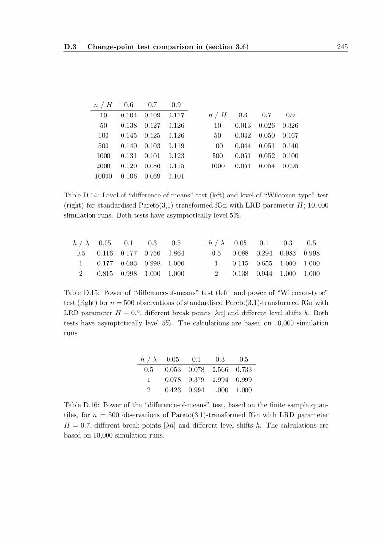
D.3 Change-point test comparison in (section 3.6) 245
n / H 0.6 0.7 0.9
10 0.104 0.109 0.117
50 0.138 0.127 0.126
100 0.145 0.125 0.126
500 0.140 0.103 0.119
1000 0.131 0.101 0.123
2000 0.120 0.086 0.115
10000 0.106 0.069 0.101
n / H 0.6 0.7 0.9
10 0.013 0.026 0.326
50 0.042 0.050 0.167
100 0.044 0.051 0.140
500 0.051 0.052 0.100
1000 0.051 0.054 0.095
Table D.14: Level of “difference-of-means” test (left) and level of “Wilcoxon-type” test
(right) for standardised Pareto(3,1)-transformed fGn with LRD parameter H; 10, 000
simulation runs. Both tests have asymptotically level 5%.
h / λ 0.05 0.1 0.3 0.5
0.5 0.116 0.177 0.756 0.864
1 0.177 0.693 0.998 1.000
2 0.815 0.998 1.000 1.000
h / λ 0.05 0.1 0.3 0.5
0.5 0.088 0.294 0.983 0.998
1 0.115 0.655 1.000 1.000
2 0.138 0.944 1.000 1.000
Table D.15: Power of “difference-of-means” test (left) and power of “Wilcoxon-type”
test (right) for n = 500 observations of standardised Pareto(3,1)-transformed fGn with
LRD parameter H = 0.7, different break points [λn] and different level shifts h. Both
tests have asymptotically level 5%. The calculations are based on 10,000 simulation
runs.
h / λ 0.05 0.1 0.3 0.5
0.5 0.053 0.078 0.566 0.733
1 0.078 0.379 0.994 0.999
2 0.423 0.994 1.000 1.000
Table D.16: Power of the “difference-of-means” test, based on the finite sample quan-
tiles, for n = 500 observations of Pareto(3,1)-transformed fGn with LRD parameter
H = 0.7, different break points [λn] and different level shifts h. The calculations are
based on 10,000 simulation runs.

246 Exact simulation results
A second set of simulations was made with Pareto(β, k) distributed observations for
β = 3, k = 1; these data have finite expectation, but an infinite variance, so that we
consider the centralized transformation
G(t) =1√Φ(t)
− 2.
• Table D.17 shows the level of both tests under standardised Pareto(2,1) dis-
tributed data. The tests are based on asymptotic critical values.
• Table D.18 shows the power of both tests under standardised Pareto(2,1) dis-
tributed data. The tests are based on asymptotic critical values.
• Since the “difference-of-means” test again does not reach its asymptotic level, we
considered its performance when it is based on finite sample quantiles as critical
values in order to compare it to the “Wilcoxon-type” test (which again already
reaches its asymptotic level when it is based on the asymptotical critical values).
The resulting power of the test is shown in Table D.16.

D.3 Change-point test comparison in (section 3.6) 247
n / H 0.6 0.7 0.9
10 0.104 0.104 0.107
50 0.159 0.138 0.120
100 0.181 0.151 0.122
500 0.223 0.148 0.124
1000 0.232 0.151 0.130
n / H 0.6 0.7 0.9
10 0.013 0.026 0.326
50 0.042 0.050 0.167
100 0.044 0.051 0.140
500 0.051 0.052 0.100
1000 0.051 0.054 0.095
Table D.17: Level of “difference-of-means” test (left) and level of “Wilcoxon-type”
test (right) for Pareto(2,1)-transformed fGn with LRD parameter H; 10, 000 simuation
runs.
h / λ 0.05 0.1 0.3 0.5
0.5 0.148 0.156 0.272 0.350
1 0.156 0.200 0.741 0.853
2 0.199 0.651 0.996 0.999
h / λ 0.05 0.1 0.3 0.5
0.5 0.075 0.180 0.878 0.960
1 0.097 0.401 0.997 1.000
2 0.122 0.744 1.000 1.000
Table D.18: Power of “difference-of-means” test (left) and power of “Wilcoxon-type”
test (right) for n = 500 observations of Pareto(2,1)-transformed fGn with LRD param-
eter H = 0.7, different break points [λn] and different level shifts h. The calculations
are based on 10,000 simulation runs.
H / n 10 50 100 500 1,000 ∞0.6 2.30 2.66 2.68 2.58 2.50 1.55
0.7 1.87 2.06 1.96 1.77 1.71 1.23
0.9 1.05 1.06 0.99 1.01 1.00 0.62
Table D.19: 5%-quantiles of the finite sample distribution of the “difference-of-means”
test under the null hypothesis for Pareto(2,1)-transformed fGn with different LRD pa-
rameter H and different sample sizes n. The calculations are based on 10,000 simulation
runs.
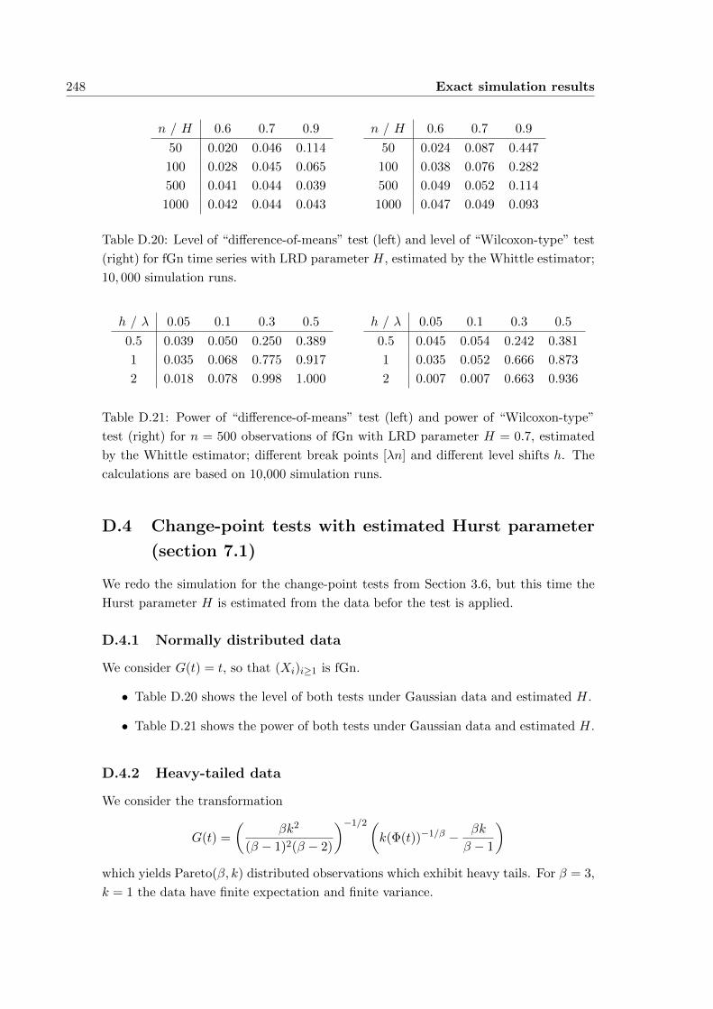
248 Exact simulation results
n / H 0.6 0.7 0.9
50 0.020 0.046 0.114
100 0.028 0.045 0.065
500 0.041 0.044 0.039
1000 0.042 0.044 0.043
n / H 0.6 0.7 0.9
50 0.024 0.087 0.447
100 0.038 0.076 0.282
500 0.049 0.052 0.114
1000 0.047 0.049 0.093
Table D.20: Level of “difference-of-means” test (left) and level of “Wilcoxon-type” test
(right) for fGn time series with LRD parameter H, estimated by the Whittle estimator;
10, 000 simulation runs.
h / λ 0.05 0.1 0.3 0.5
0.5 0.039 0.050 0.250 0.389
1 0.035 0.068 0.775 0.917
2 0.018 0.078 0.998 1.000
h / λ 0.05 0.1 0.3 0.5
0.5 0.045 0.054 0.242 0.381
1 0.035 0.052 0.666 0.873
2 0.007 0.007 0.663 0.936
Table D.21: Power of “difference-of-means” test (left) and power of “Wilcoxon-type”
test (right) for n = 500 observations of fGn with LRD parameter H = 0.7, estimated
by the Whittle estimator; different break points [λn] and different level shifts h. The
calculations are based on 10,000 simulation runs.
D.4 Change-point tests with estimated Hurst parameter
(section 7.1)
We redo the simulation for the change-point tests from Section 3.6, but this time the
Hurst parameter H is estimated from the data befor the test is applied.
D.4.1 Normally distributed data
We consider G(t) = t, so that (Xi)i≥1 is fGn.
• Table D.20 shows the level of both tests under Gaussian data and estimated H.
• Table D.21 shows the power of both tests under Gaussian data and estimated H.
D.4.2 Heavy-tailed data
We consider the transformation
G(t) =
(βk2
(β − 1)2(β − 2)
)−1/2(k(Φ(t))−1/β − βk
β − 1
)which yields Pareto(β, k) distributed observations which exhibit heavy tails. For β = 3,
k = 1 the data have finite expectation and finite variance.

D.5 Estimating Hermite coefficients (section 7.3) 249
n / H 0.6 0.7 0.9
50 0.175 0.241 0.273
100 0.212 0.286 0.269
500 0.315 0.392 0.282
1000 0.359 0.441 0.309
n / H 0.6 0.7 0.9
50 0.098 0.258 0.643
100 0.126 0.299 0.550
500 0.207 0.366 0.469
1000 0.243 0.413 0.468
Table D.22: Level of “difference-of-means” test (left) and level of “Wilcoxon-type”
test (right) for standardised Pareto(3,1)-transformed fGn with LRD parameter H, es-
timated by the Whittle estimator; 10, 000 simulation runs.
h / λ 0.05 0.1 0.3 0.5
0.5 0.378 0.472 0.882 0.939
1 0.397 0.686 0.994 0.998
2 0.437 0.794 0.999 1.000
h / λ 0.05 0.1 0.3 0.5
0.5 0.415 0.698 0.991 0.997
1 0.344 0.679 0.997 0.999
2 0.124 0.215 0.755 0.874
Table D.23: Power of “difference-of-means” test (left) and power of “Wilcoxon-type”
test (right) for n = 500 observations of standardised Pareto(3,1)-transformed fGn with
LRD parameter H = 0.7, estimated by the Whittle estimator; different break points
[λn] and different level shifts h. The calculations are based on 10,000 simulation runs.
• Table D.22 shows the level of both tests under standardised Pareto(3,1) dis-
tributed data and estimated H.
• Table D.23 shows the power of both tests under standardised Pareto(3,1) dis-
tributed data and estimated H.
D.5 Estimating Hermite coefficients (section 7.3)
We consider the model Xi = G(ξi), i = 1, . . . , n, where (ξi)i≥1 is a stationary mean-zero
Gaussian process with Var[ξi] = 1 and auto-covariance function (1.1) and a transfor-
mation G ∈ G2 which has Hermite rank m = 1. We have observed n data X1, . . . , Xn
and estimate the first Hermite coefficient
a1 = E[ξ G(ξ)],
where ξ ∼ ξ1 by
a1 =1
n
n∑i=1
ξ′(i)X(i),
where ξ′1, . . . , ξ′n are n i.i.d. standard normal distributed random variables and X(i) is
the i-th variable in the sorted sample X(1) ≤ . . . ≤ X(n) (ξ′(i) analogously).

250 Exact simulation results
Gauß Laplace(0,4) Pareto(3,1) Pareto(2,1)
n rel var rel var rel var rel var
10 0.720 0.091 0.702 0.112 0.671 0.192 0.671 3.287
50 0.911 0.021 0.904 0.031 0.885 0.109 0.844 1.085
100 0.946 0.011 0.936 0.017 0.922 0.064 0.913 1.204
500 0.982 0.002 0.981 0.004 0.971 0.021 0.955 0.270
1000 0.989 0.001 0.988 0.002 0.983 0.014 0.967 0.159
2000 0.993 0.001 0.993 0.001 0.987 0.008 0.978 0.116
5000 0.996 0.000 0.996 0.000 0.993 0.004 0.988 0.071
10000 0.998 0.000 0.998 0.000 0.995 0.003 0.994 0.039
Table D.24: Estimated Hermite coefficients a1, the mean relative to the true value a1
(rel) and the variance (var), based on 10, 000 repetitions, for different G
For 10, 000 realizations of a fGn series of length n (with Hurst parameter H = 0.7
and varying sample size n) and for different transformations G (such that normal,
Laplace and two different Pareto distributed observations arise) I have calculated a1.
Based on these each 10, 000 values, I have calculated the sample mean and the sample
variance.
• Table D.24 shows the mean of a1 relative to the true coefficient a1 as well as the
variance of a1.

D.6 Wilcoxon’s two-sample statistic (section 5.4) 251
D.6 Wilcoxon’s two-sample statistic (section 5.4)
For realizations ξ1, . . . , ξn of fGn for different Hurst parameters H, for different cutting
points λ ∈ [0, 1] and different sample sizes n, I have calculated the two-sample Wilcoxon
test statistic
UW,[λn],n =1
σW
n−2+D2
[λn]∑i=1
n∑j=[λN ]+1
(Iξi≤ξj −
1
2
)with
σ2W :=
1
4π
(λ2 − λ+ (1− λ)λ2−D + λ(1− λ)2−D) .
I have repeated this 10, 000 times for each choice of parameters n, λ,H. The results
are given
• for H = 0.6 in Table D.25,
• for H = 0.7 in Table D.26 and
• for H = 0.9 in Table D.27.
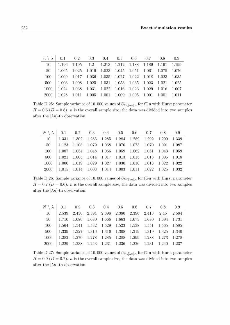
252 Exact simulation results
n \ λ 0.1 0.2 0.3 0.4 0.5 0.6 0.7 0.8 0.9
10 1.196 1.195 1.2 1.213 1.212 1.188 1.189 1.191 1.199
50 1.065 1.025 1.019 1.023 1.045 1.051 1.061 1.075 1.076
100 1.009 1.017 1.036 1.035 1.027 1.022 1.018 1.023 1.035
500 1.003 1.008 1.025 1.031 1.053 1.035 1.023 1.021 1.025
1000 1.024 1.038 1.031 1.022 1.016 1.023 1.029 1.016 1.007
2000 1.028 1.011 1.005 1.001 1.009 1.005 1.001 1.001 1.011
Table D.25: Sample variance of 10, 000 values of UW,[λn],n for fGn with Hurst parameter
H = 0.6 (D = 0.8). n is the overall sample size, the data was divided into two samples
after the [λn]-th observation.
N \ λ 0.1 0.2 0.3 0.4 0.5 0.6 0.7 0.8 0.9
10 1.331 1.302 1.285 1.285 1.284 1.289 1.292 1.299 1.339
50 1.123 1.108 1.079 1.068 1.076 1.073 1.070 1.091 1.087
100 1.087 1.054 1.048 1.066 1.059 1.062 1.051 1.043 1.059
500 1.021 1.005 1.014 1.017 1.013 1.015 1.013 1.005 1.018
1000 1.000 1.019 1.029 1.027 1.030 1.016 1.018 1.022 1.022
2000 1.015 1.014 1.008 1.014 1.003 1.011 1.022 1.025 1.032
Table D.26: Sample variance of 10, 000 values of UW,[λn],n for fGn with Hurst parameter
H = 0.7 (D = 0.6). n is the overall sample size, the data was divided into two samples
after the [λn]-th observation.
N \ λ 0.1 0.2 0.3 0.4 0.5 0.6 0.7 0.8 0.9
10 2.539 2.430 2.394 2.398 2.380 2.396 2.413 2.45 2.584
50 1.710 1.680 1.680 1.666 1.663 1.673 1.680 1.694 1.731
100 1.564 1.541 1.532 1.529 1.523 1.538 1.551 1.565 1.585
500 1.339 1.327 1.316 1.316 1.308 1.319 1.319 1.325 1.340
1000 1.282 1.270 1.278 1.285 1.288 1.299 1.288 1.273 1.278
2000 1.229 1.238 1.243 1.231 1.236 1.226 1.231 1.240 1.237
Table D.27: Sample variance of 10, 000 values of UW,[λn],n for fGn with Hurst parameter
H = 0.9 (D = 0.2). n is the overall sample size, the data was divided into two samples
after the [λn]-th observation.

List of Figures
1.1 Annual minima of the water level in the Nile river . . . . . . . . . . . . 7
1.2 Auto-correlation function of Nile river data . . . . . . . . . . . . . . . . 7
1.3 Fractional Brownian motion, looks from different distances . . . . . . . . 13
1.4 Fractional Brownian motion, different Hurst parameters . . . . . . . . . 13
1.5 Fractional Gaussian noise, different Hurst parameters . . . . . . . . . . 14
1.6 Relation between LRD behaviour of the ξi and G(ξi) . . . . . . . . . . . 14
2.1 Density of X − Y -statistic . . . . . . . . . . . . . . . . . . . . . . . . . . 31
2.2 Unnormalized variance of X − Y . . . . . . . . . . . . . . . . . . . . . . 31
2.3 X − Y for one-sample and two-sample case . . . . . . . . . . . . . . . . 32
2.4 Estimation of Var[X] . . . . . . . . . . . . . . . . . . . . . . . . . . . . . 37
2.5 Auto-covariance estimator γh, average and confidence belts . . . . . . . 38
2.6 Auto-covariance estimator γh, different realizations . . . . . . . . . . . . 38
2.7 Estimations of Var [Xm − Yn] . . . . . . . . . . . . . . . . . . . . . . . . 45
2.8 Estimations of Var [Xm − Yn], with trimmed auto-covariances . . . . . . 45
2.9 Covariance estimation influences estimation of Var [Xm − Yn] . . . . . . 46
3.1 Estimated p.d.f. and c.d.f. of sup0≤λ≤1 |Z(λ)− λZ(1)| . . . . . . . . . . 61
3.2 fGn with breaks . . . . . . . . . . . . . . . . . . . . . . . . . . . . . . . . 67
3.3 Level of “diff.-of-means” and “Wilcoxon-type” test, Gaussian data . . . 68
3.4 Power of “diff.-of-means” and “Wilcoxon-type” test, Gaussian data . . . 68
3.5 Level of “diff.-of-means” and “Wilcoxon-type” test, Laplace data . . . . 69
3.6 Power of “diff.-of-means” and “Wilcoxon-type” test, Laplace data . . . . 69
3.7 Level of “diff.-of-means” and “Wilcoxon-type” test, Pareto(3,1) data . . 70
3.8 Power of “diff.-of-means” and “Wilcoxon-type” test, Pareto(3,1) data . . 70
3.9 Power of “diff.-of-means” and “Wilcoxon-type” test, Pareto(3,1) data,
finite sample quantiles . . . . . . . . . . . . . . . . . . . . . . . . . . . . 75
3.10 Level of “diff.-of-means” and “Wilcoxon-type” test, Pareto(2,1) data . . 75
3.11 Power of “diff.-of-means” and “Wilcoxon-type” test, Pareto(2,1) data . . 76
3.12 Power of “diff.-of-means” and “Wilcoxon-type” test, Pareto(2,1) data,
finite sample quantiles . . . . . . . . . . . . . . . . . . . . . . . . . . . . 76
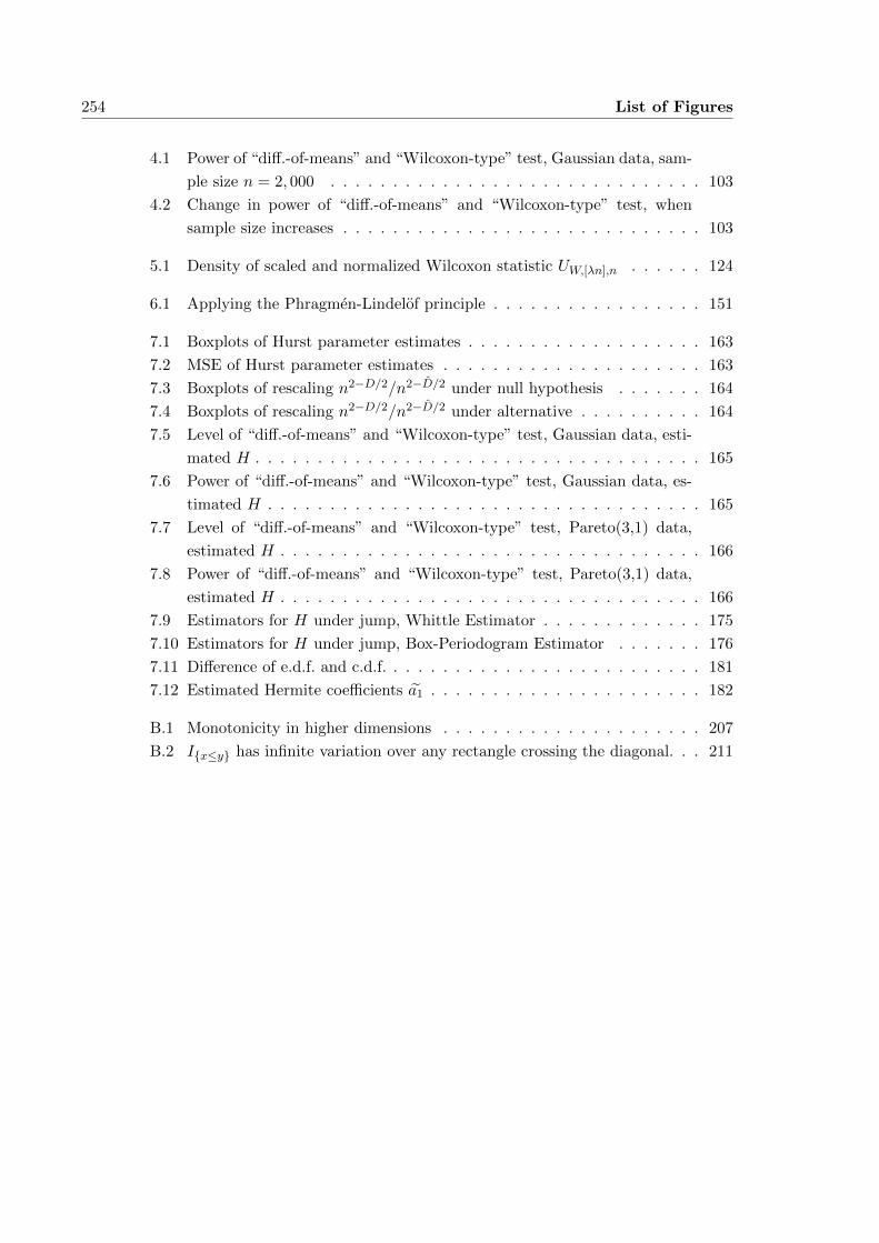
254 List of Figures
4.1 Power of “diff.-of-means” and “Wilcoxon-type” test, Gaussian data, sam-
ple size n = 2, 000 . . . . . . . . . . . . . . . . . . . . . . . . . . . . . . 103
4.2 Change in power of “diff.-of-means” and “Wilcoxon-type” test, when
sample size increases . . . . . . . . . . . . . . . . . . . . . . . . . . . . . 103
5.1 Density of scaled and normalized Wilcoxon statistic UW,[λn],n . . . . . . 124
6.1 Applying the Phragmen-Lindelof principle . . . . . . . . . . . . . . . . . 151
7.1 Boxplots of Hurst parameter estimates . . . . . . . . . . . . . . . . . . . 163
7.2 MSE of Hurst parameter estimates . . . . . . . . . . . . . . . . . . . . . 163
7.3 Boxplots of rescaling n2−D/2/n2−D/2 under null hypothesis . . . . . . . 164
7.4 Boxplots of rescaling n2−D/2/n2−D/2 under alternative . . . . . . . . . . 164
7.5 Level of “diff.-of-means” and “Wilcoxon-type” test, Gaussian data, esti-
mated H . . . . . . . . . . . . . . . . . . . . . . . . . . . . . . . . . . . . 165
7.6 Power of “diff.-of-means” and “Wilcoxon-type” test, Gaussian data, es-
timated H . . . . . . . . . . . . . . . . . . . . . . . . . . . . . . . . . . . 165
7.7 Level of “diff.-of-means” and “Wilcoxon-type” test, Pareto(3,1) data,
estimated H . . . . . . . . . . . . . . . . . . . . . . . . . . . . . . . . . . 166
7.8 Power of “diff.-of-means” and “Wilcoxon-type” test, Pareto(3,1) data,
estimated H . . . . . . . . . . . . . . . . . . . . . . . . . . . . . . . . . . 166
7.9 Estimators for H under jump, Whittle Estimator . . . . . . . . . . . . . 175
7.10 Estimators for H under jump, Box-Periodogram Estimator . . . . . . . 176
7.11 Difference of e.d.f. and c.d.f. . . . . . . . . . . . . . . . . . . . . . . . . . 181
7.12 Estimated Hermite coefficients a1 . . . . . . . . . . . . . . . . . . . . . . 182
B.1 Monotonicity in higher dimensions . . . . . . . . . . . . . . . . . . . . . 207
B.2 Ix≤y has infinite variation over any rectangle crossing the diagonal. . . 211
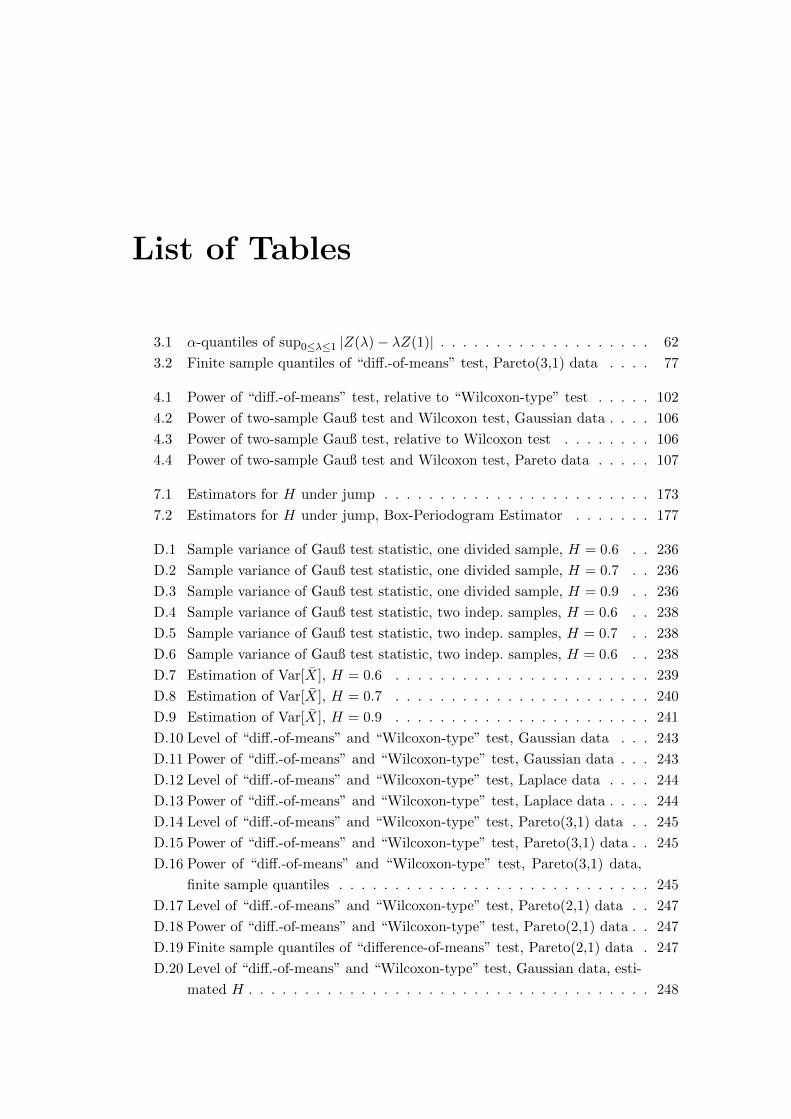
List of Tables
3.1 α-quantiles of sup0≤λ≤1 |Z(λ)− λZ(1)| . . . . . . . . . . . . . . . . . . . 62
3.2 Finite sample quantiles of “diff.-of-means” test, Pareto(3,1) data . . . . 77
4.1 Power of “diff.-of-means” test, relative to “Wilcoxon-type” test . . . . . 102
4.2 Power of two-sample Gauß test and Wilcoxon test, Gaussian data . . . . 106
4.3 Power of two-sample Gauß test, relative to Wilcoxon test . . . . . . . . 106
4.4 Power of two-sample Gauß test and Wilcoxon test, Pareto data . . . . . 107
7.1 Estimators for H under jump . . . . . . . . . . . . . . . . . . . . . . . . 173
7.2 Estimators for H under jump, Box-Periodogram Estimator . . . . . . . 177
D.1 Sample variance of Gauß test statistic, one divided sample, H = 0.6 . . 236
D.2 Sample variance of Gauß test statistic, one divided sample, H = 0.7 . . 236
D.3 Sample variance of Gauß test statistic, one divided sample, H = 0.9 . . 236
D.4 Sample variance of Gauß test statistic, two indep. samples, H = 0.6 . . 238
D.5 Sample variance of Gauß test statistic, two indep. samples, H = 0.7 . . 238
D.6 Sample variance of Gauß test statistic, two indep. samples, H = 0.6 . . 238
D.7 Estimation of Var[X], H = 0.6 . . . . . . . . . . . . . . . . . . . . . . . 239
D.8 Estimation of Var[X], H = 0.7 . . . . . . . . . . . . . . . . . . . . . . . 240
D.9 Estimation of Var[X], H = 0.9 . . . . . . . . . . . . . . . . . . . . . . . 241
D.10 Level of “diff.-of-means” and “Wilcoxon-type” test, Gaussian data . . . 243
D.11 Power of “diff.-of-means” and “Wilcoxon-type” test, Gaussian data . . . 243
D.12 Level of “diff.-of-means” and “Wilcoxon-type” test, Laplace data . . . . 244
D.13 Power of “diff.-of-means” and “Wilcoxon-type” test, Laplace data . . . . 244
D.14 Level of “diff.-of-means” and “Wilcoxon-type” test, Pareto(3,1) data . . 245
D.15 Power of “diff.-of-means” and “Wilcoxon-type” test, Pareto(3,1) data . . 245
D.16 Power of “diff.-of-means” and “Wilcoxon-type” test, Pareto(3,1) data,
finite sample quantiles . . . . . . . . . . . . . . . . . . . . . . . . . . . . 245
D.17 Level of “diff.-of-means” and “Wilcoxon-type” test, Pareto(2,1) data . . 247
D.18 Power of “diff.-of-means” and “Wilcoxon-type” test, Pareto(2,1) data . . 247
D.19 Finite sample quantiles of “difference-of-means” test, Pareto(2,1) data . 247
D.20 Level of “diff.-of-means” and “Wilcoxon-type” test, Gaussian data, esti-
mated H . . . . . . . . . . . . . . . . . . . . . . . . . . . . . . . . . . . . 248

256 List of Tables
D.21 Power of “diff.-of-means” and “Wilcoxon-type” test, Gaussian data, es-
timated H . . . . . . . . . . . . . . . . . . . . . . . . . . . . . . . . . . . 248
D.22 Level of “diff.-of-means” and “Wilcoxon-type” test, Pareto(3,1) data,
estimated H . . . . . . . . . . . . . . . . . . . . . . . . . . . . . . . . . . 249
D.23 Power of “diff.-of-means” and “Wilcoxon-type” test, Pareto(3,1) data,
estimated H . . . . . . . . . . . . . . . . . . . . . . . . . . . . . . . . . . 249
D.24 Estimated Hermite coefficients a1 . . . . . . . . . . . . . . . . . . . . . . 250
D.25 Sample variance of Wilcoxon test statistic, one divided sample, H = 0.6 252
D.26 Sample variance of Wilcoxon test statistic, one divided sample, H = 0.7 252
D.27 Sample variance of Wilcoxon test statistic, one divided sample, H = 0.9 252

Bibliography
C. R. Adams, J. A. Clarkson (1934): Properties of functions f(x, y) of bounded varia-
tion, Trans. Amer. Math. Soc., 1934, 36(4), 711–730
J. Antoch, M. Huskova, A. Janic, T. Ledwina (2008): Data driven rank tests for the
change point problem, Metrika, 2008, 68, 1–15
A. Aue, S. Hormann, L. Horvath, M. Reimherr (2009): Break detection in the co-
variance structure of multivariate time series, The Annals of Statistics, 2009, 37,
4046–4087.
J. T. Barkoulas, C. F. Baum, N. Travlos (2000): Long memory in the Greek stock
market, Applied Financial Economics, 2000, 10(2), 177–184
R. T. Baillie (1996): Long memory processes and fractional integration in econometrics,
Journal of Econometrics, 1996, 73(1), 5–59
M. Basseville, I. V. Nikiforov (1993): Detection of Abrupt Changes: Theory
and Application, Prentice-Hall Inc., Englewood Cliffs 1993, ISBN 0-13-126780-9,
http://http://www.irisa.fr/sisthem/kniga/
H. Bateman, A. Erdelyi (1953): Bateman Manuscript Project: Higher transcendental
functions, 2, McGraw-Hill Book Company Inc., New York 1953
J. Beran (1994): Statistics for Long-Memory Processes, Chapman & Hall/CRC, Boca
Raton (Florida) 1994, ISBN 0-412-04901-5
J. Beran (2010): Long-range dependence, Wiley Interdisciplinary Reviews: Computa-
tional Statistics, 2010, 2, 26–35
I. Berkes, L. Horvath, P. Kokoszka, Q.-M. Shao (2006): On discriminating between
long-range dependence and changes in the mean, The Annals of Statistics, 2006, 34,
1140–1165.
E. Beutner, W. B. Wu, H. Zahle (2012): Asymptotics for statistical functionals of long-
memory sequences, Stochastic Processes and their Applications, 122(3), 910–929
E. Beutner, H. Zahle (2011): Deriving the asymptotic distribution of U- and V-statistics
of dependent data using weighted empirical processes, Bernoulli, to appear
258 Bibliography
J. Bhan, S. Kim, J. Kim, Y. Kwon, S. Yang, K. Lee (2006): Long-range correlations in
Korean literary corpora, Chaos, Solitons & Fractals, 2006, 29(1), 69–81
N. H. Bingham, C. M. Goldie, J. L. Teugels (1989): Regular Variation, Cambridge
University Press, Cambridge 1989, ISBN 0-521-37943-1
F. J. Breidt, N. Crato, P. de Lima (1998): The detection and estimation of long memory
in stochastic volatility, Journal of Econometrics, 1998, 83(1-2), 325–348
P. Breuer, P. Major (1983): Central limit theorems for non-linear functionals of Gaus-
sian fields, Journal of Multivariate Analysis, 1983, 13(3), 425–441
B. E. Brodsky, B. S. Darkhovsky (1993): Nonparametric methods in change-point prob-
lems, Kluwer Academic Publishers, Dordrecht 1993, ISBN 0-7923-2122-7
S. V. Buldyrev, A. L. Goldberger, S. Havlin, R. N. Mantegna, M. E. Matsa, C.-K. Peng,
M. Simons, H. E. Stanley (1995): Long-range correlation properties of coding and
noncoding DNA sequences: GenBank analysis, Phys. Rev. E, 1995, 51(5), 5084–5091
R. Caballero, S. Jewson, A. Brix (2002): Long memory in surface air temperature: de-
tection, modeling, and application to weather derivative valuation, Climate Research,
2002, 21, 127–140
O. Cappe, E. Moulines, J.-C. Pesquet, A. Petropulu, X. Yang (2002): Long-range de-
pendence and heavy-tail modeling for teletraffic data, IEEE Signal Processing Mag-
azine, 2002, 19(3), 14–27
Y. Chen, M. Ding, J. A. S. Kelso (1997): Long Memory Processes (1/fα Type) in
Human Coordination, Physical Review Letters, 79(22), 4501–4504
Y.-W. Cheung (1993): Long memory in foreign exchange rates, Journal of Business
and Economic Statistics, 1993, 11, 93–101
Y.-W. Cheung, K. S. Lai (1995): A search for long memory in international stock
market returns, Journal of International Money and Finance, 1995, 14(4), 597–615
J. A. Clarkson, C. R. Adams (1933): On definitions of bounded variation for functions
of two variables, Trans. Amer. Math. Soc., 1933, 35(4), 824–854
M. Csorgo, L. Horvath (1988): Invariance Principle for Changepoint Problems, Journal
of Multivariate Analysis, 1988, 27, 151–168
M. Csorgo, L. Horvath (1997): Limit Theorems in Change-Point Analysis, John Wiley
& Sons, Chichester 1997, ISBN 0-471-95522-1
H. Dehling, R. Fried (2010): Asymptotic Distribution of Two-Sample Empirical U-
Quantiles with Applications to Robust Tests for Structural Change, SFB 823 Dis-
cussion Paper, 2010, 43

Bibliography 259
H. Dehling, A. Rooch, M. S. Taqqu (2012): Nonparametric Change-Point Tests for
Long-Range Dependent Data. Scand. J. Stat., 2012, to appear
H. Dehling, A. Rooch, M. S. Taqqu (2013): Power of Change-Point Tests for Long-
Range Dependent Data. preprint, 2013
H. Dehling, M. S. Taqqu (1989): The Empirical process of some long-range dependent
sequences with an application to U -statistics, Ann. Stat., 1989, 17(4), 1767–1783
H. Dehling, M. S. Taqqu (1991): Bivariate symmetric statistics of long-range dependent
observations, Journal of Statistical Planning and Inference, 1991, 28, 153–165
R. L. Dobrushin, P. Major (1979): Non-Central Limit Theorems for Non-Linear Func-
tionals of Gaussian Fields, Z. Wahrscheinlichkeitstheorie verw. Gebiete, 1979, 50(1),
27–52
A. Erramilli, O. Narayan, W. Willinger (1996): Experimental queueing analysis with
long-range dependent packet traffic, IEEE/ACM Transactions on Networking, 1996,
4(2), 209–223
K. Fritzsche, H. Grauert (2002): From Holomorphic Functions to Complex Manifolds,
Springer, New York 2002, ISBN 978-0-387-95395-3
T. Geisel, J. Nierwetberg, A. Zacherl (1985): Accelerated Diffusion in Josephson Junc-
tions and Related Chaotic Systems, Phys. Rev. Lett., 1985, 54(7), 616–619
L. Giraitis, R. Leipus, D. Surgailis (1996): The change-point problem for dependent
observations, J. Statist. Plann. Inference, 53, 297–310
L. Giraitis, M. S. Taqqu (1999): Whittle Estimator for Finite-Variance Non-Gaussian
Time Series with Long Memory, The Annals of Statistics, 1999, 27(1), 178–203
K. Grochenig (2001): Foundations of Time-Frequency Analysis, Birkhauser, Boston
2001, ISBN 978-0-817-64022-4
H. Heuser (2003): Lehrbuch der Analysis, Teil 1, 15th edition, B.G. Teubner GmbH,
Stuttgart 2003, ISBN 3-519-62233-5
G. H. Hardy (1905): On double Fourier series, and especially those with represent the
double zeta-function with real and incommensurable parameters, Quart. J. of Math.,
1905, 37, 53–79
U. Hassler, M. Olivares (2007): Long memory and structural change: New evidence
from German stock market returns, unpublished
U. Hassler, J. Scheithauer (2009): Detecting Changes from Short to Long Memory.
Statistical Papers, 2011, 52(4), 847–870
260 Bibliography
L. Horvath, P. Kokoszka (1997): The effect of long-range dependence on change-point
estimators, J. Statist. Plann. Inference, 64, 57–81
T. Hsing, W. B. Wu (2004): On weighted U-statistics for stationary processes, Ann.
Probab., 2004, 32(2), 1600–1631
C.-C. Hsu (2005): Long memory or structural changes: An empirical examination on
inflation rates, Economics Letters, 2005, 88(2), 289–294
H. Hurst (1951): Long Term Storage Capacity of Reservoirs, Transactions of the Amer-
ican Society of Civil Engineers, 1951, 116, 770–799
H. Hurst (1955): Methods of using long-term storage in reservoirs, Proceedings of the
Institution of Civil Engineers, 1955, part I, 519–577
K. Ito (1951): Multiple Wiener Integral, J. Math. Soc. Japan, 1951, 3, 157–169
R. Kannan, C. K. Krueger (1996): Advanced Analysis: On the Real Line, Springer,
New York 1996, ISBN 978-0-387-94642-9
T. Karagiannis, M. Faloutsos, R. H. Riedi (2002): Long-Range Dependence: Now you
see it, now you don’t!, Global Telecommunications Conference, 2002, 3, 2165–2169
T. Karagiannis, M. Molle, M. Faloutsos (2004): Long-Range Dependence, Ten Years
of Internet Traffic Modeling, IEEE Internet Computing, 2004, 8(5), 57–64
P. Kokoszka, R. Leipus (1998): Change-point in the mean of dependent observations,
Stat. & Prob. Letters, 40, 385–393
W. Kramer, P. Sibbertsen (2002): Testing for Structural Changes in the Persistence of
Long Memory. International Journal of Business and Economics, 1, 235–242
W. Kramer, P. Sibbertsen, C. Kleiber (2002): Long memory versus structural change
in financial time series, Allgemeines Statistisches Archiv, 2002, 86, 83–96
H. R. Kunsch (1987): Statistical aspects of self-similar processes, in: Yu. A. Prohorov,
V.V. Sazonov (eds.), Proceedings of the First World Congres of the Bernoulli Society,
1, 67–74, VNU Science Press, Utrecht
H.-H. Kuo (2006): Introduction to Stochastic Integration, Springer, New York 2006,
ISBN 978-0-387-28720-1
H. Kuswanto (2009): A New Simple Test Against Spurious Long Memory Using Tem-
poral Aggregation Heri Kuswanto, Discussion Paper, Wirtschaftswissenschaftliche
Fakultat der Leibniz Universitat Hannover, No. 425
J. W. Lamperti (1962): Semi-stable stochastic processes, Trans. Am. Math. Soc., 1962,
104, 62–78

Bibliography 261
M. J. Lebo, R. W. Walker, H. D. Clarke (2000): You must remember this: dealing with
long memory in political analyses, Electoral Studies, 2000, 19(1), 31–48
E. Lehmann (1975): Nonparametrics: Statistical Methods Based on Ranks, Holden-Day,
San Francisco
J. B. Levy, M. S. Taqqu (2000): Renewal Reward Processes with Heavy-Tailed Inter-
Renewal Times and Heavy-Tailed Rewards, Bernoulli, 2000, 6(1), 23–44
Q. Li, D. L. Mills (1998): On the Long-range Dependence of Packet Round-trip Delays
in Internet, In Proceedings of IEEE ICC98, 1998, 1185–1191
S. Ling (2007): Testing for change points in time series models and limiting theorems
for NED sequences, The Annals of Statistics, 2007, 35, 1213–1227
F. Lillo, S. Mike, J. D. Farmer (2005): Theory for long memory in supply and demand,
Physical Review E, 2005, 71(6), 066122-1–066122-11
P. Major (1981a): Multiple Wiener-Ito Integrals, Lecture Notes in Mathematics 849,
Springer, Berlin Heidelberg 1981
P. Major (1981b): Limit theorems for non-linear functionals of Gaussian sequences,
Z.Wahrscheinlichkeitstheorie und verw. Gebiete, 1981, 57, 129–158
B. B. Mandelbrot, J. W. van Ness (1968): Fractional Brownian Motions, Fractional
Noises and Applications, SIAM Review, 1968, 10(4), 422–437
B. B. Mandelbrot, J. R. Wallis (1969a): Computer Experiments With Fractional Gaus-
sian Noises, Water Ressources Research, 1969, 5(1), 228–241
B. B. Mandelbrot, J. R. Wallis (1969b): Some long-run properties of geophysical
records, Water Ressources Research, 1969, 5(2), 321–340
F. Moricz (1976): Moment inequalities and the strong laws of large numbers, Z.
Wahrscheinlichkeitstheorie verw. Gebiete, 1976, 35(4), 299–314
M. A. Montemurro, P. A. Pury (2002): Long-range fractal correlations in literary cor-
pora, Fractals, 2002, 10(4), 451–461
B. Øksendal (1998): Stochastic Differential Equations, 5th edition, Springer, Berlin
Heidelberg 1998, ISBN 3-540-63720-6
A. Ott, J.P. Bouchaud, D. Langevin, W. Urbach (1990): Anomalous diffusion in “living
polymers”: A genuine Levy flight?, Phys. Rev. Lett., 1990, 65(17), 2201–2204
A. B. Owen (2004): Multidimensional variation for quasi-Monte Carlo, Technical Re-
port, Department of Statistics, Stanford University, 2004, no. 2004-02
262 Bibliography
C. K. Peng, S. V. Buldyrev, A. L. Goldberger, S. Havlin, F. Sciortino, M. Simons and
H. E. Stanley (1992): Long-range correlations in nucleotide sequences, Nature, 1992,
359, 168–170
C.-K. Peng, S. V. Buldyrev, S. Havlin, M. Simons, H. E. Stanley, and A. L. Goldberger
(1994): Mosaic organization of DNA nucleotides, Phys. Rev. E, 1994, 49(2), 1685–
1689
V. Pipiras, M. S. Taqqu (2011): Long Range Dependence and Self-Similarity, preprint
Y. A. Rozanov (1967): Stationary Random Processes, Holden-Day, San Francisco 1967
G. Samorodnitsky (2007): Long Range Dependence, Now Publishers, Hanover 2007,
ISBN 978-1-60198-090-8
G. Samorodnitsky, M. S. Taqqu (1994): Non-Gaussian Stable Processes: Stochastic
Models with Infinite Variance, Chapman and Hall, London, 1994
X. Shao (2011): A simple test of changes in mean in the possible presence of long-range
dependence, Journal of Time Series Analysis, 2011, 32(6), 598–606
G. R. Shorack, J. A. Wellner (1986): Empirical Processes with Applications to Statistics,
John Wiley & Sons, New York 1986, ISBN 0-471-86725-X
P. Sibbertsen (2004): Long Memory versus Structural Breaks: An Overview, Statistical
Papers, 2004, 45, 465–515
P. Sibbertsen, J. Willert (2010): Testing for a Break in Persistence under Long-Range
Dependencies and Mean Shifts, Statistical Papers, 2010
B. Simon (1974): The P (Φ)2 Euclidean (Quantum) field theory, Princeton University
Press, Princeton 1974, ISBN 0-691-08144-1
R. L. Smith (1993): Long-Range Dependence and Global Warming, in: R. A. Madden,
R. W. Katz: Applications of Statistics to Modeling the Earth’s Climate System, 1994,
89–92
D. Surgailis (2003): CLTs for Polynomials of Linear Sequences: Diagram Formula
with Illustrations, in: P. Doukhan, G. Oppenheim, M. S. Taqqu (eds.): Theory and
Applications of Long-Range Dependence, Birkhauser, Boston Basel Berlin 2003, ISBN
0-817-64168-8
M. S. Taqqu (1975): Weak Convergence to Fractional Brownian Motion and to the
Rosenblatt Process, Z. Wahrscheinlichkeitstheorie verw. Gebiete, 1975, 31, 287–302
M. S. Taqqu (1979): Convergence of Integrated Processes of Arbitrary Hermite Rank,
Z. Wahrscheinlichkeitstheorie verw. Gebiete, 1979, 50, 53–83
Bibliography 263
M. S. Taqqu (2003): Fractional Brownian Motion and Long-Range Dependence, in: P.
Doukhan, G. Oppenheim, M. S. Taqqu (eds.): Theory and Applications of Long-
Range Dependence, Birkhauser, Boston Basel Berlin 2003, ISBN 0-817-64168-8
M. S. Taqqu (2012): personal communication
M. S. Taqqu, V. Teverovsky (1998): On Estimating the Intensity of Long-Range De-
pendence in Finite and Infinite Variance Time Series, in: R. Adler, R. Feldmann,
M. S. Taqqu (eds.): A Practical Guide To Heavy Tails: Statistical Techniques and
Applications, Birkhauser, Boston 1998, 177–217
M. S. Taqqu, V. Teverovsky, W. Willinger (1995): Estimators for long-range depen-
dence: an emprical study, Fractals, 1995, 3, 785–798
M. S. Taqqu, W. Willinger, R. Sherman (1997): Proof of a fundamental result in
self-similar traffic modelling, ACM/SIGCOMM Computer Communications Review,
1997, 27, 5–23
V. Teverovsky, M. Taqqu (1997): Testing for long-range dependence in the presence of
shifting means or a slowly declining trend, using a variance-type estimator, J. Time
Ser. Anal., 1997, 18, 279–304
E. C. Titchmarsh (1964): The Theory of Functions, 2nd edition, Oxford University
Press 1964, ISBN 0-198-53349-7
C. Varotsos, D. Kirk-Davidoff (2006): Long-memory processes in ozone and tempera-
ture variation at the region 60 S–60 N, Atmospheric Chemistry and Physics, 2006,
6(12), 4093–4100
M. K. Vemuri (2008): Hermite expansions and Hardy’s theorem, arXiv:0801.2234v1
[math.AP], 2008
W. H. Young (1913): On Multiple Fourier Series, Proc. London Math. Soc. (2), 1913,
11, 133–184
W. H. Young (1916): On multiple integration by parts and the second theorem of the
mean, Proc. London Math. Soc. (2), 1916, 16, 273–293
L. Wang (2003): Limit theorems in change-point problems with multivariate long-range
dependent observations, Statistics & Decisions, 21(3), 283–300
L. Wang (2008a): Change-in-mean problem for long memory time series models with
applications, J. Statist. Computat. Simul., 78(7), 653–668
L. Wang (2008b): Change-point detection with rank statistics in long-memory time-
series models, Aust. N. Z. J. Stat., 50(3), 241–256

264 Bibliography
E. W. Weisstein (2010): Hermite Polynomial, MathWorld–A Wolfram Web Resource,
http://mathworld.wolfram.com/HermitePolynomial.html, 2010-09-01
D. Wied, W. Kramer, H. Dehling (2011): Testing for a change in correlation at an
unknown point in time using an extended functional delta method, Econometric
Theory, to appear
N. Wiener (1938): The homogeneous chaos, Amer. J. Math., 1938, 60, 897–936
W. Willinger, M. S. Taqqu, R. Sherman, D. V. Wilson (1997): Self-similarity through
High-Variability: Statistical Analysis of Ethernet LAN Traffic at the Source Level,
IEEE/ACM Transaction on Networking, 1997, 5(1), 71–86
W. Willinger, M. S. Taqqu, V. Teverovsky (1999): Stock market prices and long-range
dependence, Finance and Stochastics, 1999, 3(1), 1–13