FNRM 5262 - Final Project

CHANGE DETECTION ANALYSIS USING

REMOTE SENSING TECHNIQUES

Change in Urban area from 1992 to 2001 in COIMBATORE, INDIA.

- Shoumith Jeyakumar

INTRODUCTION:

Coimbatore, also known as the Manchester of the south, is located at the southern

part of India, within the state of Tamil Nadu. It is the second largest city and urban

agglomeration in the state after its capital [Chennai] and the sixteenth largest urban

agglomeration of India. It is one of the fastest growing tier-II cities in India and a

major textile, industrial, commercial, educational, information technology,

healthcare and manufacturing hub of Tamil Nadu.

Due to large scale industrialisation and growth of the Information Technology sector

over the last two decades, there has been a variation in the population within the

city boundaries, owing to rapid urban development. The population within the

Coimbatore city conglomeration according to the census of India for the years 1991,

2001 and 2011 are 1,100,746; 1,461,139 and 2,136,916 respectively.

[http://www.citypopulation.de/India-TamilNadu.html] There has been an expansion

of the boundary of the urban area over time.

The goal of my project is to identify the urban sprawl for this city over time using

satellite imagery. Landsat imagery for this area for the years 1992 and 2001 was

obtained. The images were classified using unsupervised classification technique and

change detection was performed to see the change in the urban class during the

duration of 9 years.

Study Area Map: [Source: google maps]

STEPS FOLLOWED:

The steps that were followed to achieve the results are listed below.

- Obtaining Imagery.

- Subset.

- Classification.

- Recoding.

- Change Detection.

- Summary results.

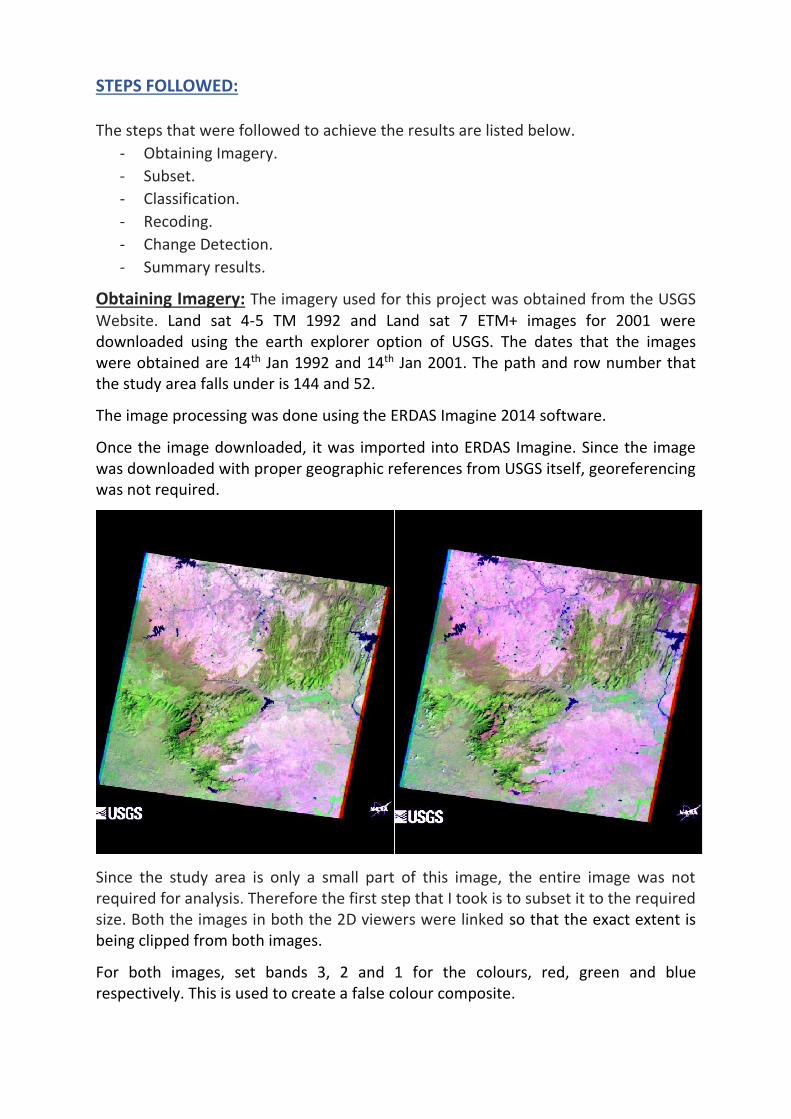
Obtaining Imagery: The imagery used for this project was obtained from the USGS

Website. Land sat 4-5 TM 1992 and Land sat 7 ETM+ images for 2001 were downloaded using the earth explorer option of USGS. The dates that the images were obtained are 14th Jan 1992 and 14th Jan 2001. The path and row number that the study area falls under is 144 and 52.

The image processing was done using the ERDAS Imagine 2014 software.

Once the image downloaded, it was imported into ERDAS Imagine. Since the image was downloaded with proper geographic references from USGS itself, georeferencing was not required.

Since the study area is only a small part of this image, the entire image was not required for analysis. Therefore the first step that I took is to subset it to the required size. Both the images in both the 2D viewers were linked so that the exact extent is being clipped from both images.

For both images, set bands 3, 2 and 1 for the colours, red, green and blue respectively. This is used to create a false colour composite.

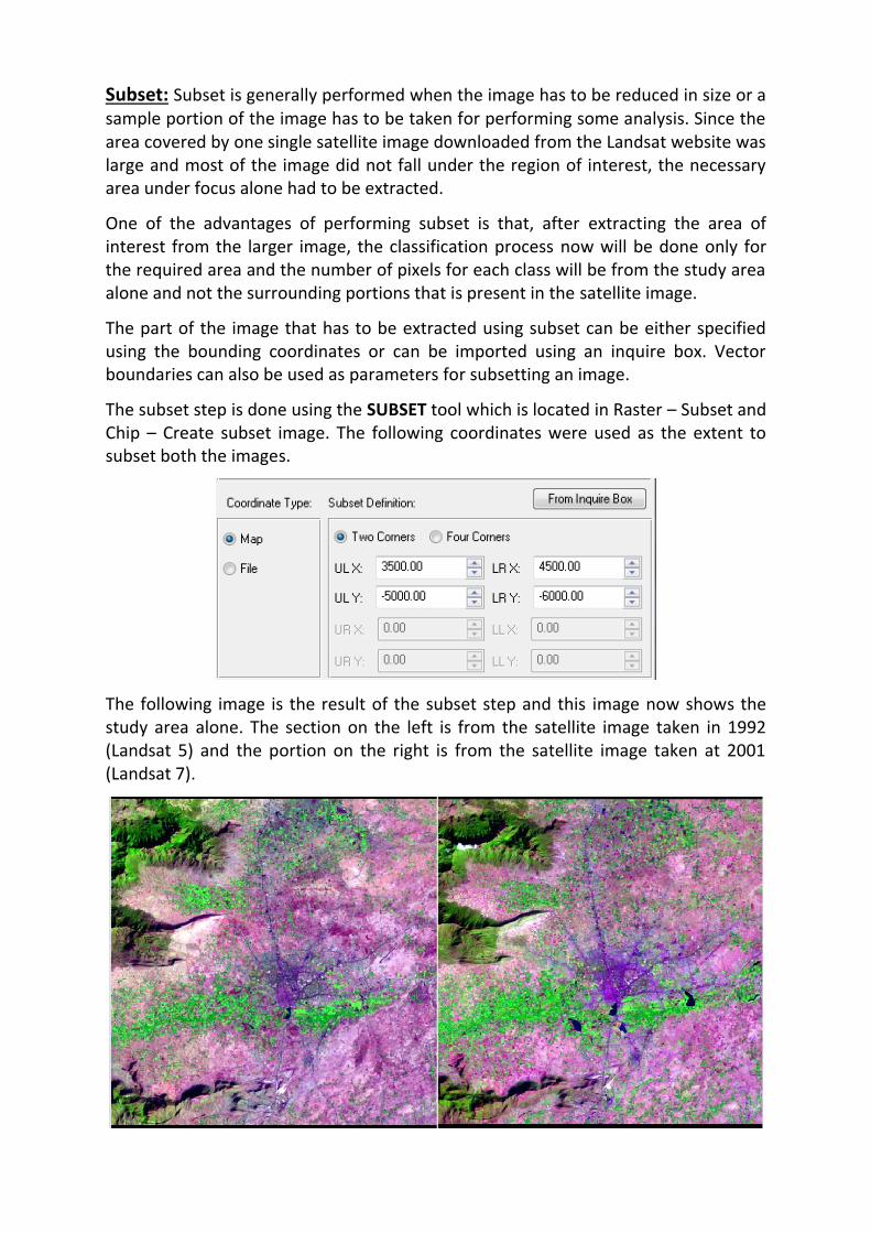
Subset: Subset is generally performed when the image has to be reduced in size or a sample portion of the image has to be taken for performing some analysis. Since the area covered by one single satellite image downloaded from the Landsat website was large and most of the image did not fall under the region of interest, the necessary area under focus alone had to be extracted.

One of the advantages of performing subset is that, after extracting the area of interest from the larger image, the classification process now will be done only for the required area and the number of pixels for each class will be from the study area alone and not the surrounding portions that is present in the satellite image.

The part of the image that has to be extracted using subset can be either specified using the bounding coordinates or can be imported using an inquire box. Vector boundaries can also be used as parameters for subsetting an image.

The subset step is done using the SUBSET tool which is located in Raster – Subset and Chip – Create subset image. The following coordinates were used as the extent to subset both the images.

The following image is the result of the subset step and this image now shows the study area alone. The section on the left is from the satellite image taken in 1992 (Landsat 5) and the portion on the right is from the satellite image taken at 2001 (Landsat 7).

Classification: In order to do change detection, the image has to be classified into appropriate classes first. Classification is the process of assorting the pixels into different classes on Land Use and Land cover based on characteristics of the light reflected from each of the LULC type in the area that this image covers.

There are two methods that can be used to perform Classification. One is the unsupervised classification where the software categorizes the pixels into distinct classes based on the number of classes specified by the user. The other method is where the user creates training classes/pixels where he/she specifies the type of pixels that falls under each class based on his/her knowledge of the area. The software then uses these samples and compares it with the rest of the image to match the characteristics and thus classifies the entire image.

The method that was chosen to follow for this project is UNSUPERVISED CLASSIFICATION. This method was chosen as there was lack of proper knowledge of the area, training pixels could not be created and associated to the right classes with accuracy. Since the unsupervised classification is computer automated, it was more preferable.

The output of the unsupervised classification first performed on Landsat 5 TM image is shown above. The number of desired classes was set to 15 and the number of iterations was set to 25.

Several different outputs were obtained by setting different desired number of classes while performing the classification and different iterations numbers were used to try and improve the accuracy of the classification process. After analysing the different outputs that were obtained, the classes that fall under “Urban” category were identified, color-coded differently and renamed.

The same procedure was followed in classifying the Landsat 7 ETM+ image and the urban classes were identified on that image as well.

The final classification outputs for both the images are shown below. The image on the left is the classified output of Landsat 5 TM taken in 1992 and the image on the right is the classified output of Landsat 7 ETM+ image taken in 2001.

From the images above, it can be clearly seen that there is a lot of change in the urban area between the two time periods that are considered. It is clearly seen that the concentration of the urban class had become dense in the central business district area of the city.

Recoding: Recoding is the process of reclassification of the classes. This is done by combining them based on similar characteristics and having a more general class. For example, the unsupervised classification may have resulted in 5 different classes within the forest area which may have been due to the different types of canopy cover within the forest. But if the user wants a general forest class and does not require the categorisation into sub classes, then the user performs recoding.

The goal of this project is to identify the change of the urban class alone. Therefore recoding was performed in such a way that every other class except the urban ones were categorized into one general non-urban class and the value of it was set to 0. The urban classes were set to the value 1. On doing this, it was easier to focus on the desired class alone.

After recoding both the classified output images and setting the appropriate colour for the class, the output obtained is shown below. These images which are the result of the recoding step are the ones that are to be used as input in the following change detection step.

Change Detection: Change detection is defined as a process used to identify the

change that occurred in a specific area over a span of time. By observing the same area at different time intervals using satellites or Aerial photography, the user can identify the change of land use and land cover in that area. Several other analysis can also be done with the help of change detection techniques such as change in the condition of the water or the degrading of a plant species etc.

There are several methods to perform change detection using satellite images such as image differencing, Principal Component Analysis, Image Regression etc. Most methods use statistical calculations to compare the brightness values of the pixels present in the two images and produce results.

Since the images used for this study were already classified, the Post classification comparison method was used. This is a simple and more promising method which produces accurate results if the classification is done accurately.

Since the images taken at the different times were already independently classified, these classified images can be used to produce change maps that will visualise the pixels that have changed from one class to another.

The following image shows the output of this step (on the left) in comparison with the two input images (on the right). The grey portion in the 2D viewer shows the pixels that have changed from one class to another in the duration of 10 years.

These change detection results can be summarised into a report to show the number of pixels changed from non-urban class to the urban class, the percentage of total pixels that have changed and also the area of change in Hectares.

Summary report: The summary report of the matrix option is used to obtain the

report that shows the overall change in percentage and also the change of area in hectares.

The input zone file was set to the reclassification result of the Landsat 5 image and the input class file was set to the reclassification result of the Landsat 7 TM image. From the interactive output option, it is possible to see the change of pixels from one class to the other and also the change of percentage and the change of area in Hectares.

The pixel change count values are recorded in an excel table to make it easier to interpret.

From this, we can see the number of pixels that has changed from one class to another.

RESULTS AND DISCUSSION:

The following image shows the change pixels that have changed from the non-urban class to the urban class over the period of 9 years.

From the above summary, it is possible to see that there is a moderate amount of change from one class to another. The change from the non-urban class to the urban class totals up to an area of 3.71 hectares.

From the image above, it is possible to visually interpret that there is more densification of the urban class pixels within the same area when compared to the any expansion of the urban cluster.

From the knowledge I have about this area from living here during this time span, I have seen the development within the city, with new residential and commercial areas being built in the locations which were once green spaces (parks, barren land, banana plantation, corn plantations). It is also easy to interpret rom the image that there has been development along the roadway corridor (a line from the cluster in the middle going north). In India, it is common to set up shops and stores on the sides of roads. Since that road was converted to a full-fledged highway, there was rapid development along this corridor.

A few assumptions were made while doing this change detection analysis. During recoding the classes from the initial unsupervised classification step into urban and non-urban, it was done with the assumption that the classes that had pixels that were within only the major urban cluster and nowhere else belonged to the urban class. There were a few hilly regions on the north-west region of the image. There were a few pixels that had the characteristics of an urban class along the foot of the hills. Since my focus was on the central portion of the city more than the regions that lie in the outskirts, these classes along the foot of the hills were also considered non-urban.

Accuracy Assessment could not be done because I was not able to find a high resolution image for this area.

SOURCES:

1. http://earthexplorer.usgs.gov/ – Used to obtain Landsat imagery. 2. www.maps.google.com – Used to obtain the map for the study area. 3. www.wikipedia.com – Used to obtain general information about the city. 4. http://www.citypopulation.de/India-TamilNadu.html - Obtained population

information. 5. ERDAS Imagine Help – Used to figure out how to use the tools within the

software.