Ch. 8 Comparative-Static Analysis of General-Function Models
61
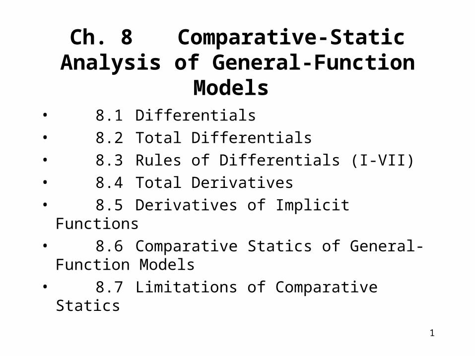
1 Ch. 8 Comparative-Static Analysis of General-Function Models • 8.1 Differentials • 8.2 Total Differentials • 8.3 Rules of Differentials (I-VII) • 8.4 Total Derivatives • 8.5 Derivatives of Implicit Functions • 8.6 Comparative Statics of General- Function Models • 8.7 Limitations of Comparative Statics
description
Ch. 8 Comparative-Static Analysis of General-Function Models. 8.1Differentials 8.2Total Differentials 8.3Rules of Differentials (I-VII) 8.4Total Derivatives 8.5Derivatives of Implicit Functions 8.6Comparative Statics of General-Function Models - PowerPoint PPT Presentation
Transcript of Ch. 8 Comparative-Static Analysis of General-Function Models
1
Ch. 8 Comparative-Static Analysis of General-Function
Models • 8.1 Differentials• 8.2 Total Differentials• 8.3 Rules of Differentials (I-VII)• 8.4 Total Derivatives• 8.5 Derivatives of Implicit Functions• 8.6 Comparative Statics of General-
Function Models• 8.7 Limitations of Comparative
Statics
2
011
1)9
01
1
1
1)8
01
1
1)7
1006)
1005)
4)
xoperator with derivative partiallim)3
2)
such thatother affect the w/oitselfby can vary each x
another one oft independen all are xvariables)1
167 p. s,Derivative Partial 4.7
00
111
10
111
i1
2
2
btb
tT
Gtb-b
-b)d(taG)t(IT
btb
t)b(C
Gtb-b
a-bdG)-t)(Ib(C
btbY
Gtb-b
GI a-bdY
) t ; (d tY; dT
) b ; (a b(Y-T); a C
G I C Y
fyx
ΔxΔy
Δx),x,Δx,xf(xΔxΔy
),x,,xf(xy
*
o
*
*
o
*
*
o
*
Δx
n
n
3
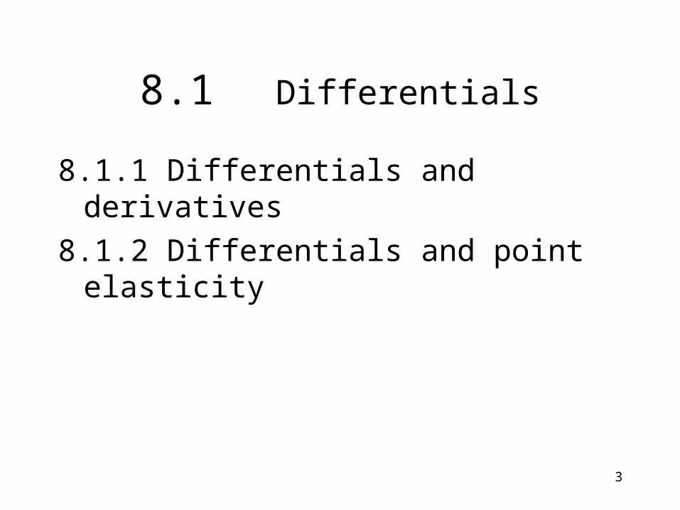
8.1Differentials
8.1.1 Differentials and derivatives8.1.2 Differentials and point
elasticity
4
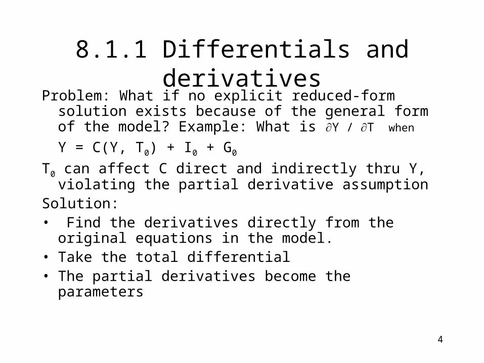
8.1.1 Differentials and derivatives
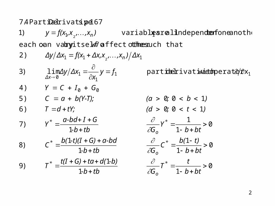
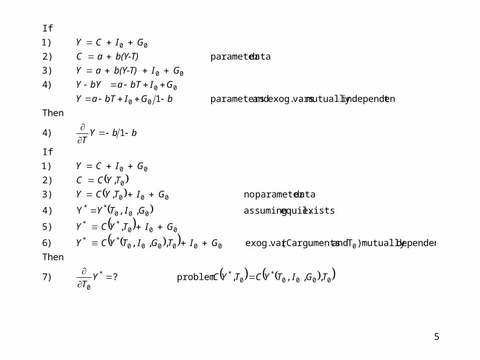
Problem: What if no explicit reduced-form solution exists because of the general form of the model? Example: What is Y / T when
Y = C(Y, T0) + I0 + G0
T0 can affect C direct and indirectly thru Y, violating the partial derivative assumption
Solution:• Find the derivatives directly from the
original equations in the model.• Take the total differential • The partial derivatives become the
parameters
5
TG ITYCTYCYT
G ITG ITY C Y
G ITY C Y
G ITY
G ITY CY
TY CC
G I C Y
bbYT
bGIbTaY
GIbTabYY
G I b(Y-T) a Y
b(Y-T) a C
G I C Y
0000*
0**
0
0000000**
000**
000**
000
0
00
00
00
00
00
,,,, :problem?)7
Then
dependentmutually )T and arguments (C var exog. ,,,)6
,5)
exists equil. assuming,,Y4)
dataparameter no,3)
,2)
1)
If
1)4
Then
tindependenmutually varsexog. and parameters1
)4
3)
dataparameter 2)
1)
If
6
xxfy
xxxfxfxf
xf
dxxfdy
xxxfy
xxxfy
xfxy
xxfxy
xyxfydx
dx
0
01001
1
0
)8
)7
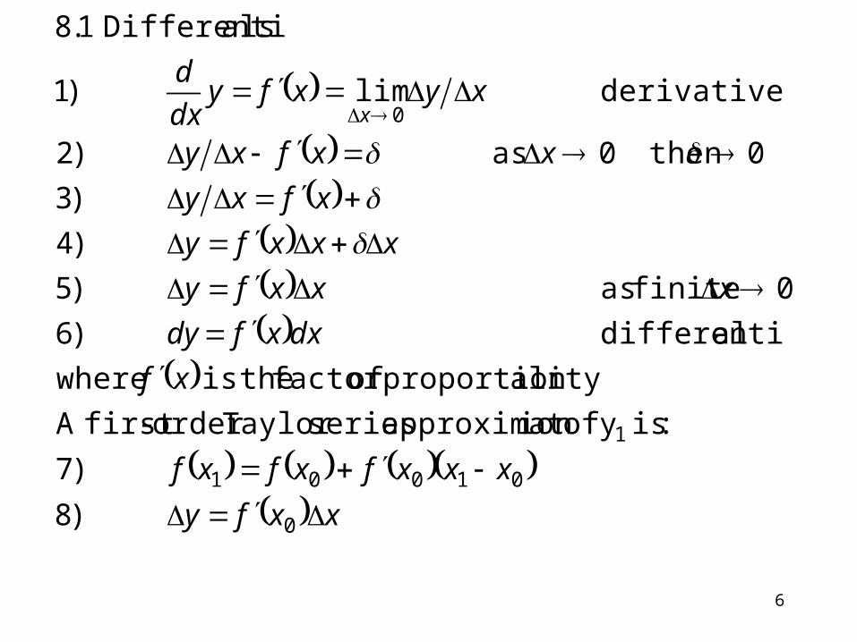
:is y ofion approximat seriesTaylor order -firstA
alityproportion offactor theis where
aldifferenti)6
0 finite as)5
)4
)3
0 then 0 as)2
derivativelim)1
alsDifferenti 1.8
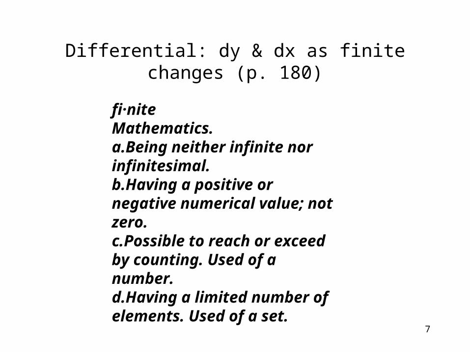
Differential: dy & dx as finite changes (p. 180)
7
fi·nite Mathematics. a.Being neither infinite nor infinitesimal. b.Having a positive or negative numerical value; not zero. c.Possible to reach or exceed by counting. Used of a number. d.Having a limited number of elements. Used of a set.
8
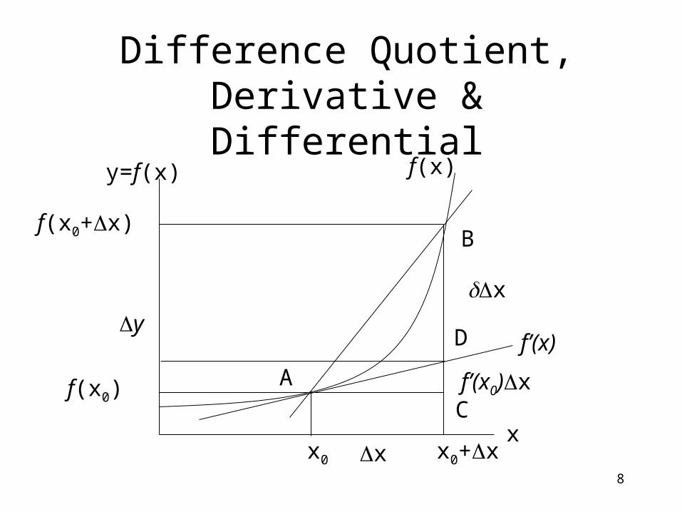
Difference Quotient, Derivative & Differential
f(x0+x)
f(x)
f(x0)
x0 x0+x
y=f(x)
x
y
x
f’(x)
f’(x0)x
x
A
C
D
B
9
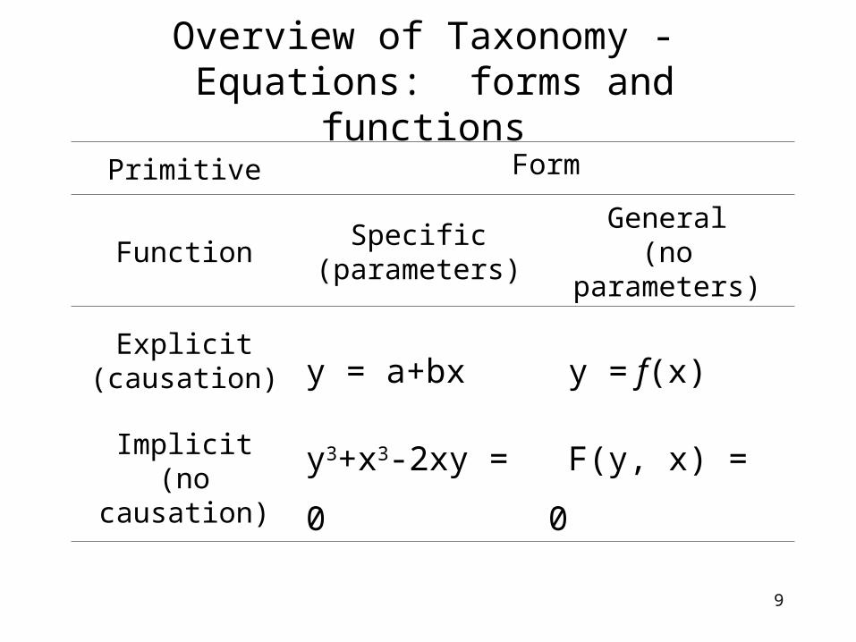
Overview of Taxonomy - Equations: forms and functions
Primitive Form
FunctionSpecific
(parameters)General
(no parameters)
Explicit(causation) y = a+bx y = f(x)
Implicit(no causation) y3+x3-2xy = 0 F(y, x) = 0
10
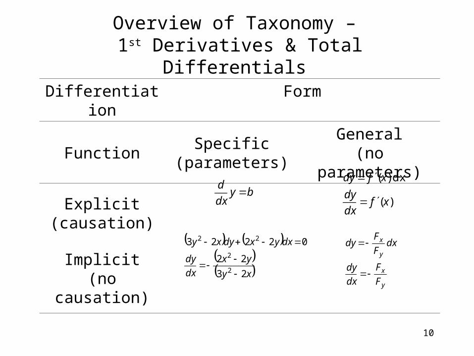
Overview of Taxonomy – 1st Derivatives & Total Differentials
Differentiation Form
FunctionSpecific
(parameters)General
(no parameters)
Explicit(causation)
Implicit(no causation)
bydx
d
)(
dx )(
xfdx
dy
xfdy
xy
yx
dx
dy
dxyxdyxy
23
22
02223
2
2
22
y
x
y
x
F
F
dx
dy
dxF
Fdy
11
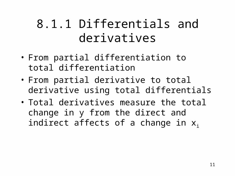
8.1.1 Differentials and derivatives
• From partial differentiation to total differentiation
• From partial derivative to total derivative using total differentials
• Total derivatives measure the total change in y from the direct and indirect affects of a change in xi
12
8.1.1 Differentials and derivatives
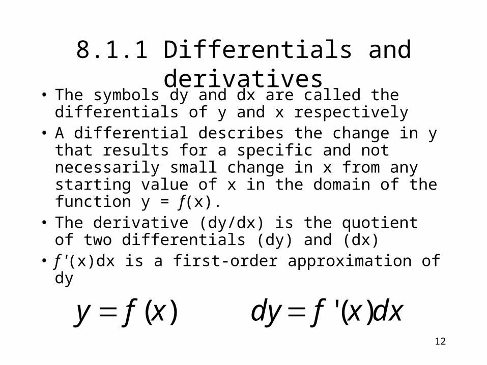
• The symbols dy and dx are called the differentials of y and x respectively
• A differential describes the change in y that results for a specific and not necessarily small change in x from any starting value of x in the domain of the function y = f(x).
• The derivative (dy/dx) is the quotient of two differentials (dy) and (dx)
• f '(x)dx is a first-order approximation of dy
dxxfdyxfy )(')(
13
8.1.1 Differentials and derivatives
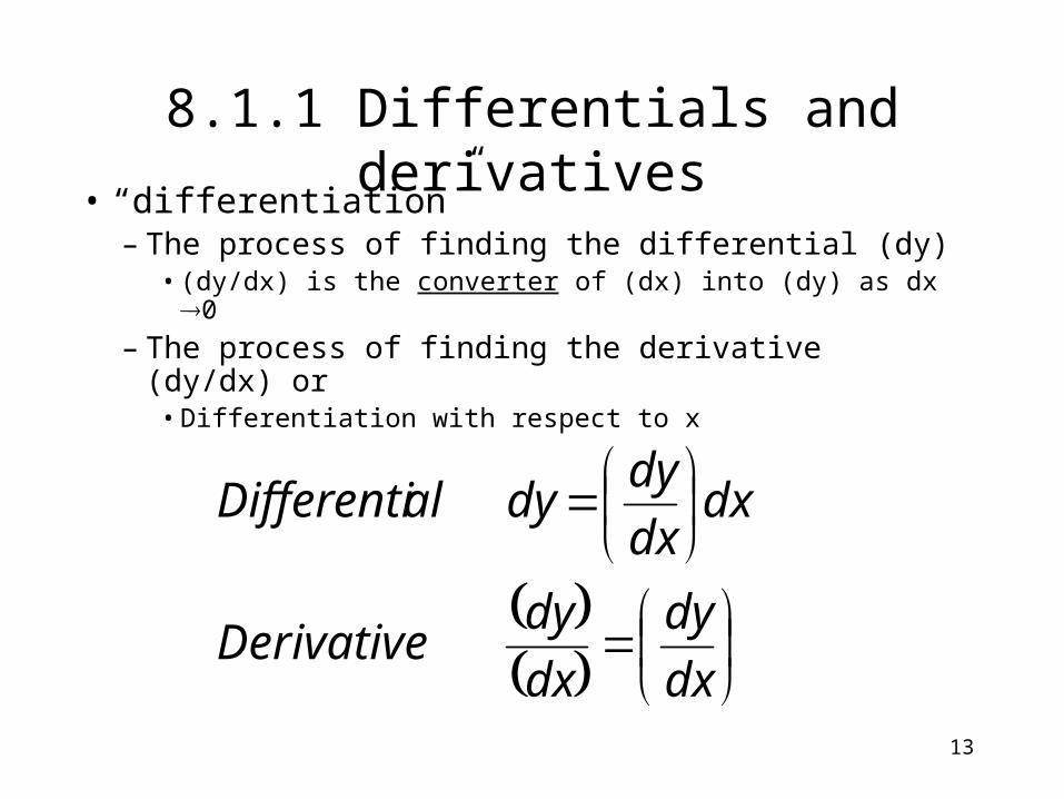
• “differentiation”– The process of finding the differential (dy)
• (dy/dx) is the converter of (dx) into (dy) as dx 0
– The process of finding the derivative (dy/dx) or• Differentiation with respect to x
dx
dy
dx
dyDerivative
dxdx
dydyalDifferenti
14
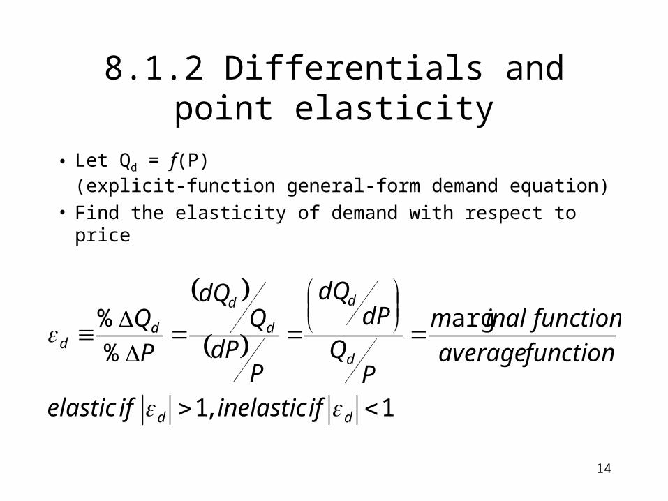
8.1.2 Differentials and point elasticity
• Let Qd = f(P) (explicit-function general-form demand equation)
• Find the elasticity of demand with respect to price
1,1
arg
%
%
dd
d
d
d
d
dd
ifinelasticifelastic
functionaverage
functioninalm
PQ
dPdQ
PdP
QdQ
P
Q
15
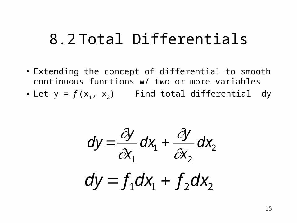
8.2 Total Differentials
• Extending the concept of differential to smooth continuous functions w/ two or more variables
• Let y = f (x1, x2) Find total differential dy
22
11
dxx
ydx
x
ydy
2211 dxfdxfdy
16
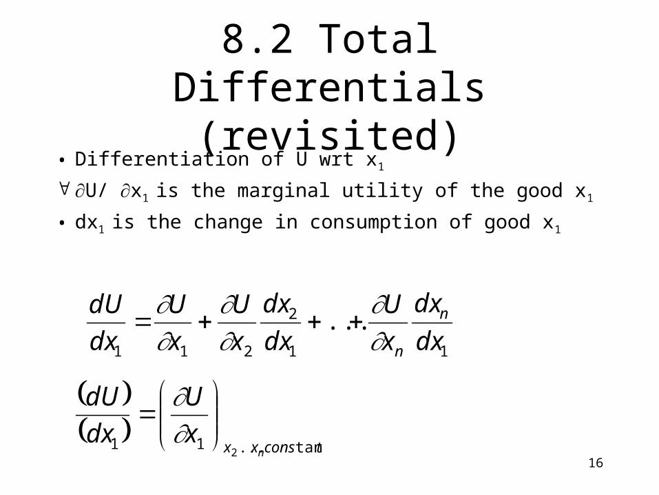
8.2 Total Differentials (revisited)
• Differentiation of U wrt x1
U/ x1 is the marginal utility of the good x1
• dx1 is the change in consumption of good x1
tconsxx nx
U
dx
dU
tan...112
11
2
211
...dx
dx
x
U
dx
dx
x
U
x
U
dx
dU n
n
17
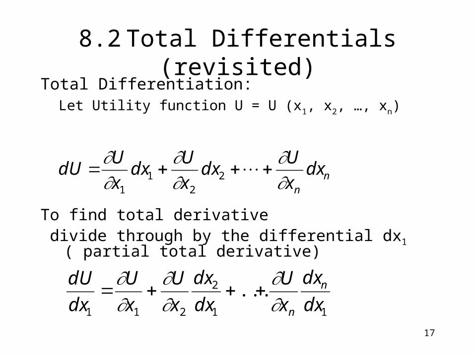
8.2 Total Differentials (revisited)
Total Differentiation: Let Utility function U = U (x1, x2, …, xn)
nn
dxx
Udx
x
Udx
x
UdU
22
11
11
2
211
...dx
dx
x
U
dx
dx
x
U
x
U
dx
dU n
n
To find total derivative divide through by the differential dx1 ( partial
total derivative)
18
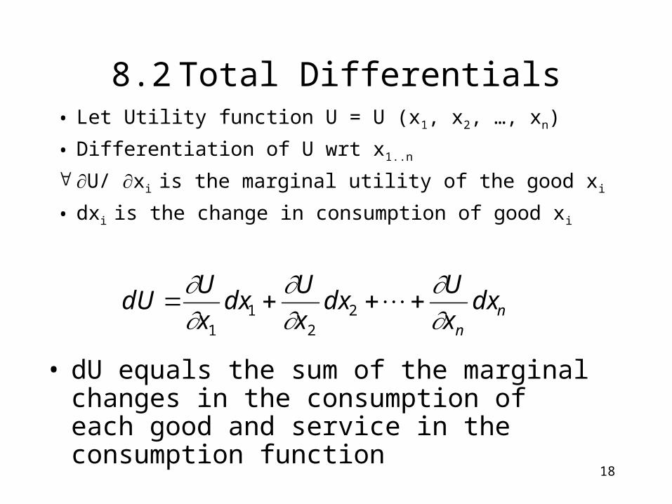
8.2 Total Differentials• Let Utility function U = U (x1, x2, …, xn)
• Differentiation of U wrt x1..n
U/ xi is the marginal utility of the good xi
• dxi is the change in consumption of good xi
nn
dxx
Udx
x
Udx
x
UdU
22
11
• dU equals the sum of the marginal changes in the consumption of each good and service in the consumption function
19
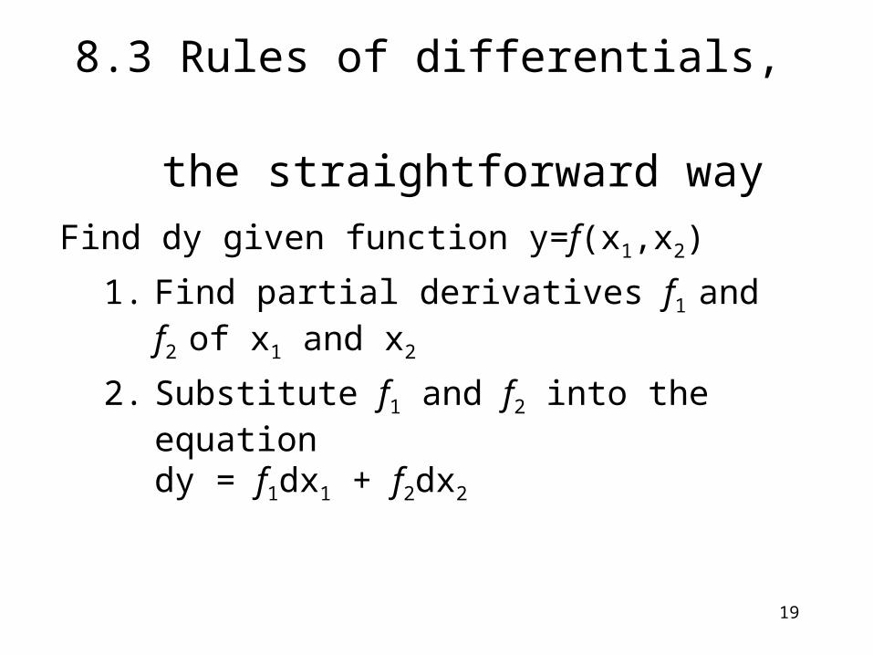
8.3 Rules of differentials, the straightforward way
Find dy given function y=f(x1,x2)
1. Find partial derivatives f1 and f2 of x1 and x2
2. Substitute f1 and f2 into the equationdy = f1dx1 + f2dx2
20
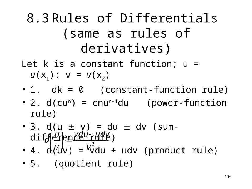
8.3 Rules of Differentials (same as rules of derivatives)
Let k is a constant function; u = u(x1); v = v(x2)
• 1. dk = 0 (constant-function rule)• 2. d(cun) = cnun-1du (power-function rule)• 3. d(u v) = du dv (sum-difference
rule)• 4. d(uv) = vdu + udv (product rule)• 5. (quotient rule)
2v
udvvdu
v
ud
21
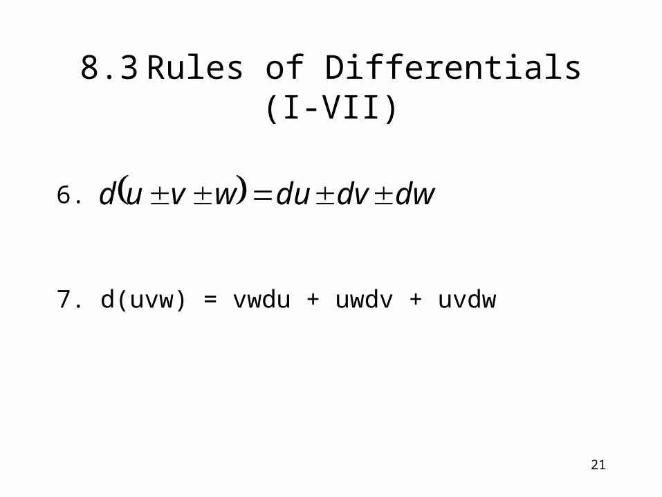
8.3 Rules of Differentials (I-VII)
6.
7. d(uvw) = vwdu + uwdv + uvdw
dwdvduwvud
22
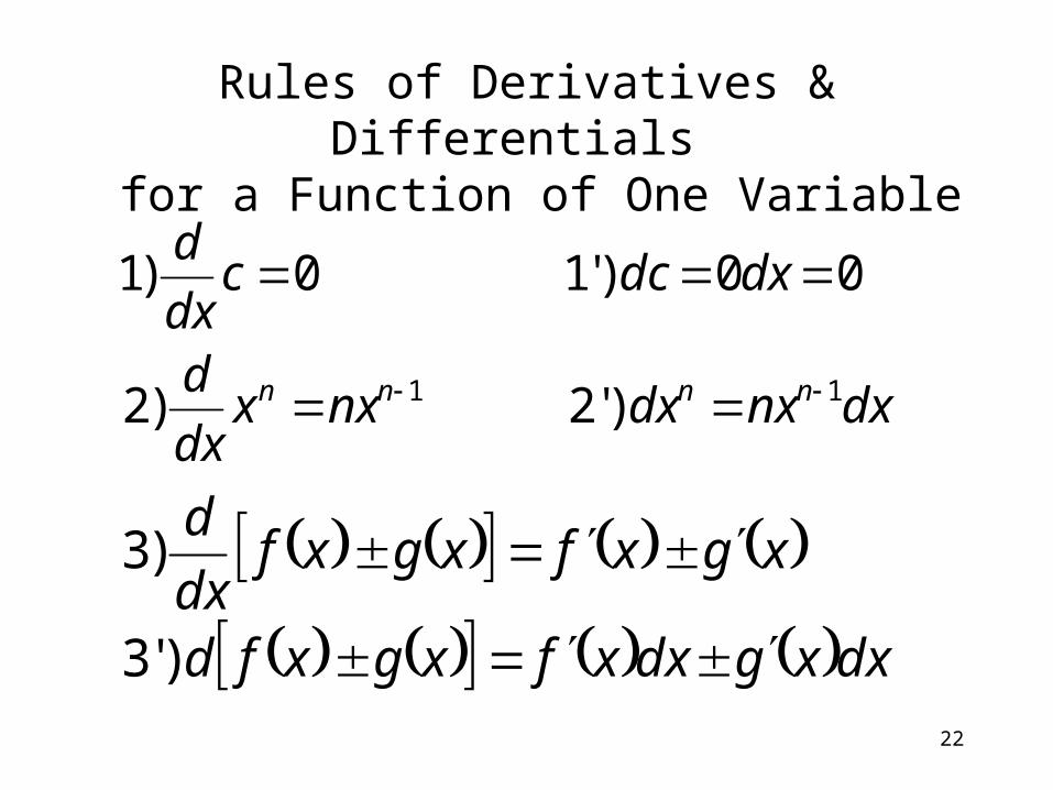
Rules of Derivatives & Differentials for a Function of One Variable
dxnxdxnxxdx
d
dxdccdx
d
nnnn 11 )'2)2
00)'10)1
dxxgdxxfxgxfd
xgxfxgxfdx
d
)'3
)3
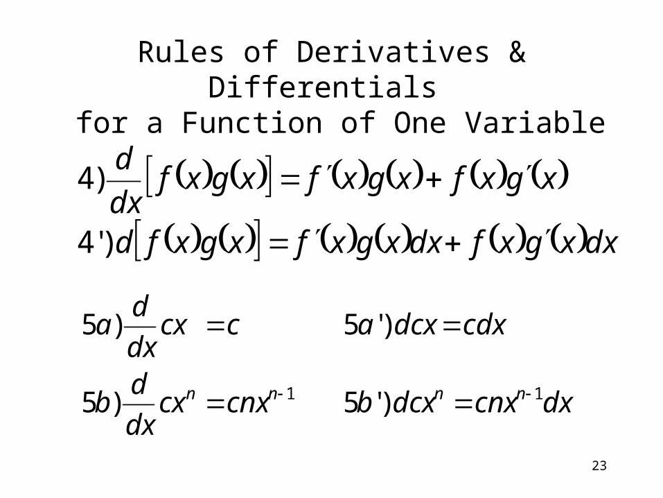
23
Rules of Derivatives & Differentials for a Function of One Variable
dxxgxfdxxgxfxgxfd
xgxfxgxfxgxfdx
d
)'4
)4
dxcnxdcxbcnxcxdx
db
cdxdcxaccxdx
da
nnnn 11 )'5)5
)'5)5
24
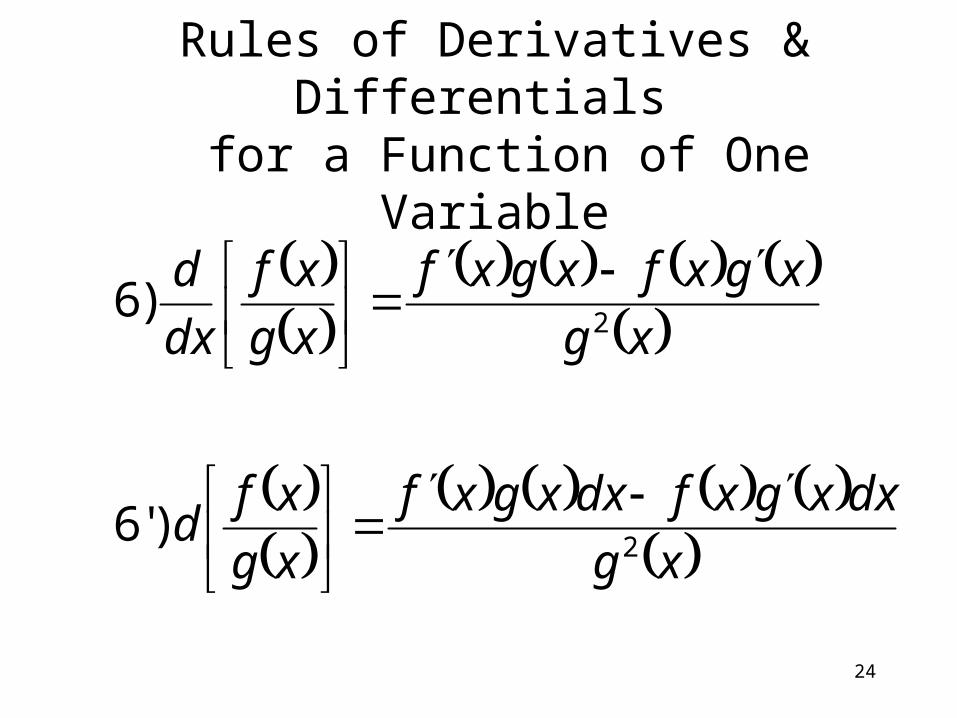
xg
dxxgxfdxxgxf
xg
xfd
xg
xgxfxgxf
xg
xf
dx
d
2
2
)'6
)6
Rules of Derivatives & Differentials
for a Function of One Variable
25
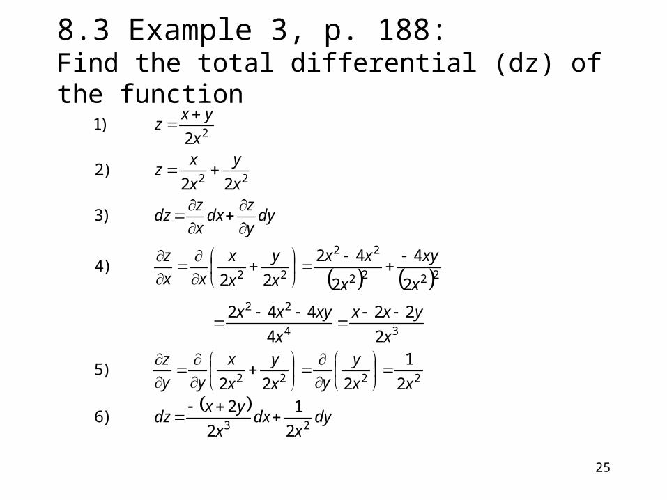
8.3 Example 3, p. 188: Find the total differential (dz) of the function
dy
xdx
x
yxdz
xx
y
yx
y
x
x
yy
zx
yxx
x
xyxx
x
xy
x
xx
x
y
x
x
xx
z
dyy
zdx
x
zdz
x
y
x
xz
x
yxz
23
2222
34
22
2222
22
22
22
2
2
1
2
2)6
2
1
222 )5
2
22
4
442
2
4
2
42
22)4
)3
22)2
2 )1
26
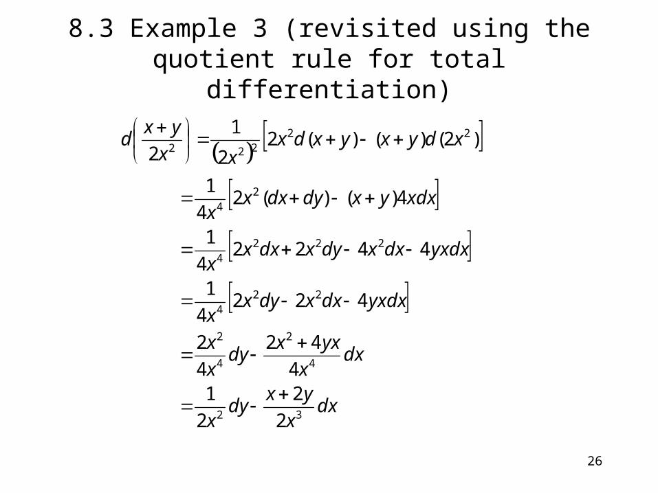
8.3 Example 3 (revisited using the quotient rule for total differentiation)
dxx
yxdy
x
dxx
yxxdy
x
x
yxdxdxxdyxx
yxdxdxxdyxdxxx
xdxyxdydxxx
xdyxyxdxxx
yxd
32
4
2
4
2
224
2224
24
22222
2
2
2
14
42
4
2
4224
1
44224
1
4)()(24
1
)2()()(22
1
2
27
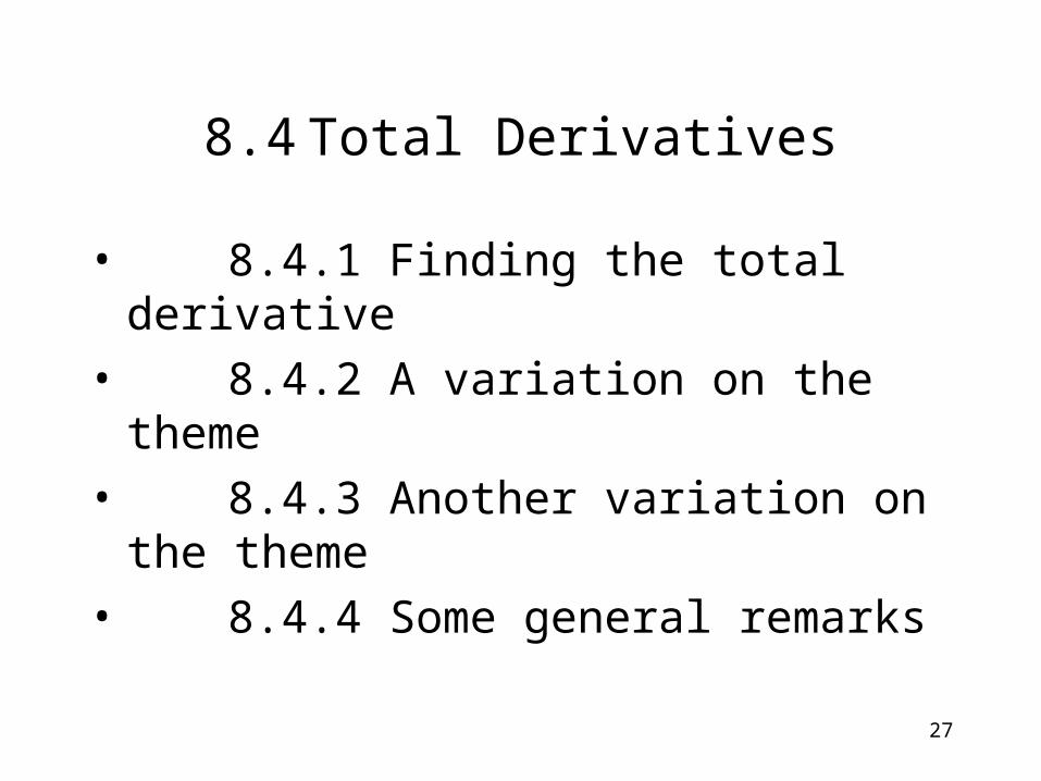
8.4 Total Derivatives
• 8.4.1 Finding the total derivative
• 8.4.2 A variation on the theme• 8.4.3 Another variation on the
theme• 8.4.4 Some general remarks
28
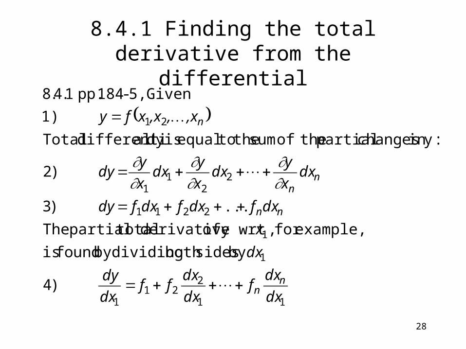
8.4.1 Finding the total derivative from the differential
11
221
1
1
1
2211
22
11
21
)4
by sidesboth dividingby found is
example,for ,y wrt of derivative totalpartial The
...)3
)2
:yin changes partial theof sum the toequal isdy aldifferenti Total
1)
Given 5,-184 pp. 1.4.8
dx
dxf
dx
dxff
dx
dy
dx
x
dxfdxfdxfdy
dxx
ydx
x
ydx
x
ydy
,x,,xxfy
nn
nn
nn
n
29
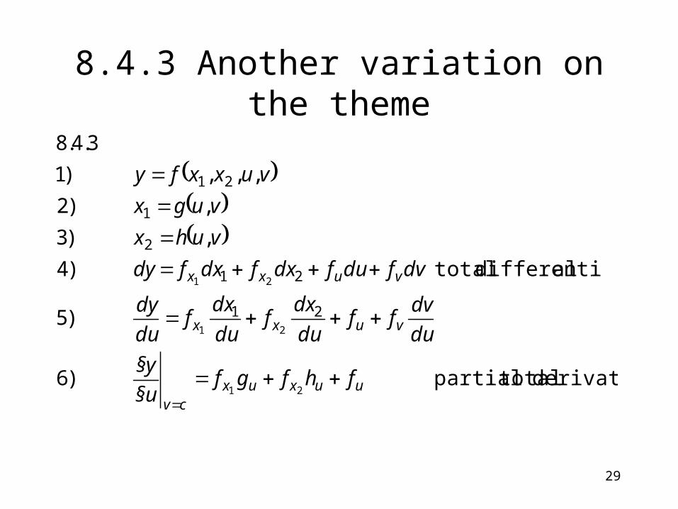
8.4.3 Another variation on the theme
derivative totalpartial)6
)5
aldifferenti total)4
,)3
,)2
,,,)1
3.4.8
21
21
21
21
21
2
1
21
uuxuxcv
vuxx
vuxx
fhfgf§u
§y
du
dvff
du
dxf
du
dxf
du
dy
dvfdufdxfdxfdy
vuhx
vugx
vuxxfy
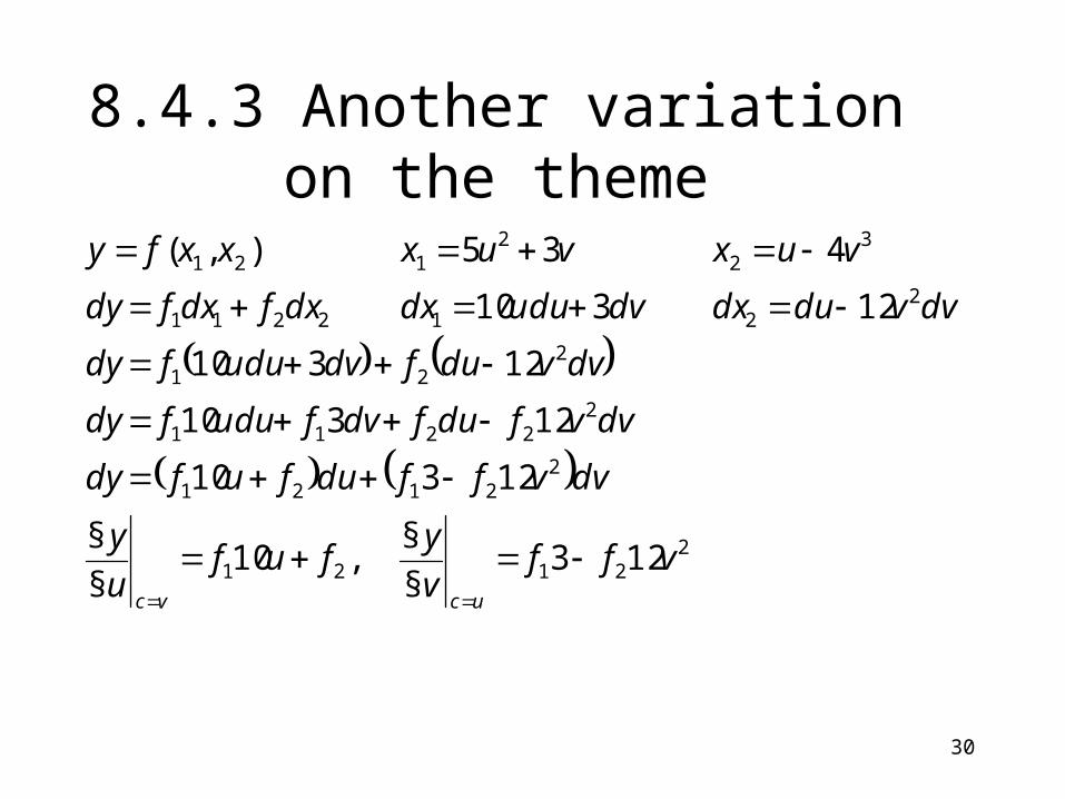
30
2
2121
22121
22211
221
2212211
32
2121
123§
§,10
§
§
12310
12310
12310
12310
435),(
vffv
yfuf
u
y
dvvffdufufdy
dvvfdufdvfudufdy
dvvdufdvudufdy
dvvdudxdvududxdxfdxfdy
vuxvuxxxfy
ucvc
8.4.3 Another variation on the theme
31
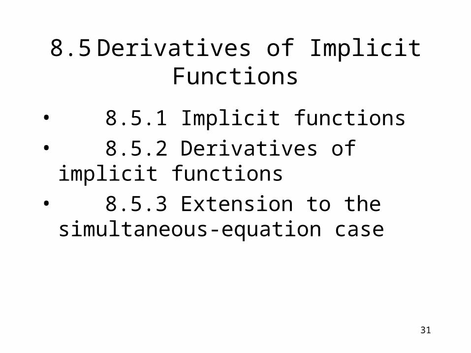
8.5 Derivatives of Implicit Functions
• 8.5.1 Implicit functions• 8.5.2 Derivatives of implicit
functions• 8.5.3 Extension to the
simultaneous-equation case
32
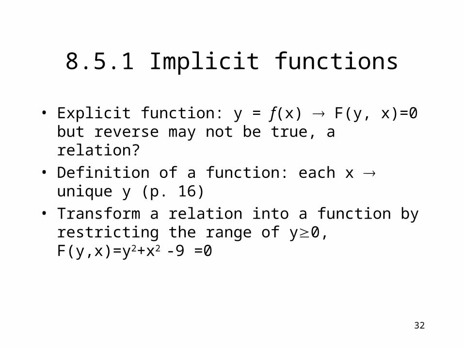
8.5.1 Implicit functions
• Explicit function: y = f(x) F(y, x)=0 but reverse may not be true, a relation?
• Definition of a function: each x unique y (p. 16)
• Transform a relation into a function by restricting the range of y0, F(y,x)=y2+x2 -9 =0
33
8.5.1 Implicit functions
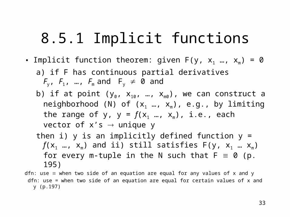
• Implicit function theorem: given F(y, x1 …, xm) = 0
a) if F has continuous partial derivativesFy, F1, …, Fm and Fy 0 and
b) if at point (y0, x10, …, xm0), we can construct a neighborhood (N) of (x1 …, xm), e.g., by limiting the range of y, y = f(x1 …, xm), i.e., each vector of x’s unique y
then i) y is an implicitly defined function y = f(x1 …, xm) and ii) still satisfies F(y, x1 … xm) for every m-tuple in the N such that F 0 (p. 195)
dfn: use when two side of an equation are equal for any values of x and y
dfn: use = when two side of an equation are equal for certain values of x and y (p.197)
34
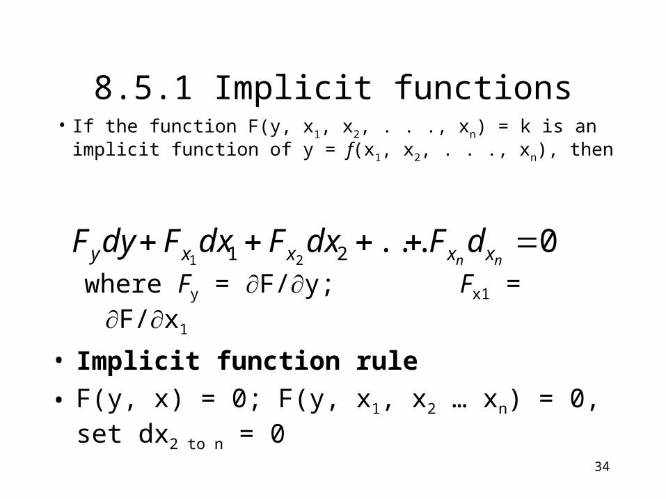
8.5.1 Implicit functions• If the function F(y, x1, x2, . . ., xn) = k is an
implicit function of y = f(x1, x2, . . ., xn), then
where Fy = F/y; Fx1 = F/x1
• Implicit function rule
• F(y, x) = 0; F(y, x1, x2 … xn) = 0, set dx2
to n = 0
0...21 21
nn xxxxy dFdxFdxFdyF
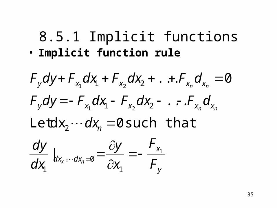
35
8.5.1 Implicit functions• Implicit function rule
y
xdxdx
n
xxxxy
xxxxy
F
F
x
y
dx
dy
dx
dFdxFdxFdyF
dFdxFdxFdyF
nx
nn
nn
1
21
21
10.
1
2
21
21
|
such that 0dxLet
...
0...
36
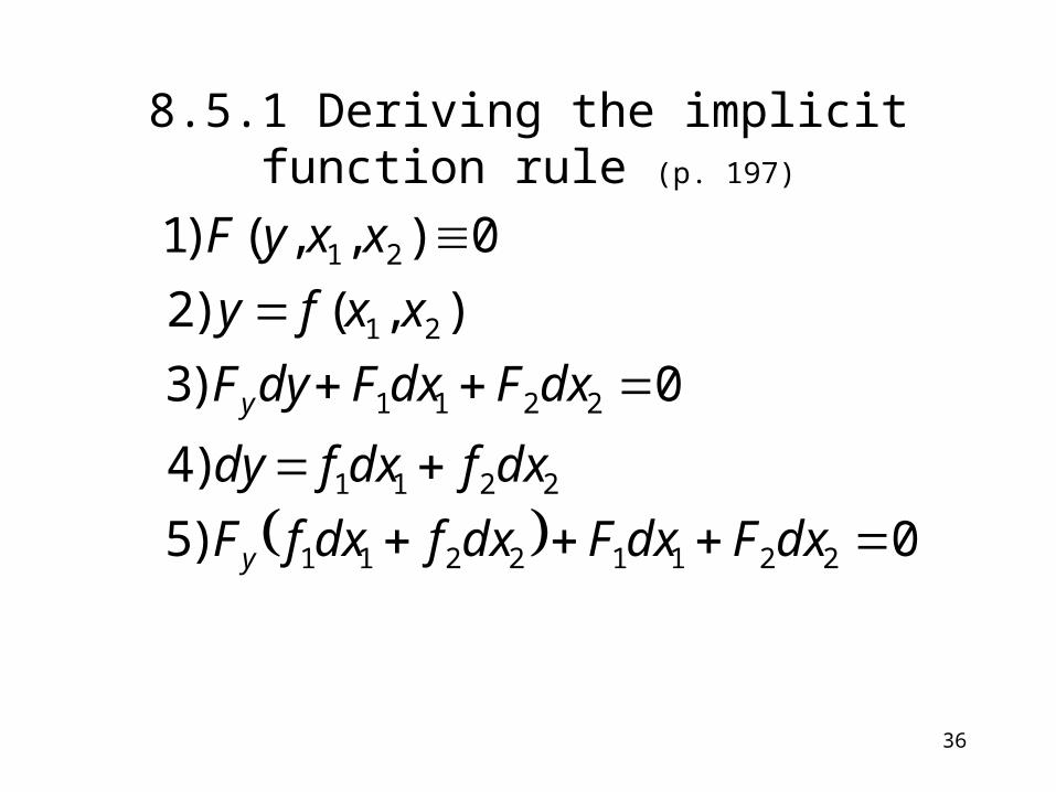
8.5.1 Deriving the implicit function rule (p. 197)
0)5
)4
0)3
),()2
0),,()1
22112211
2211
2211
21
21
dxFdxFdxfdxfF
dxfdxfdy
dxFdxFdyF
xxfy
xxyF
y
y
37
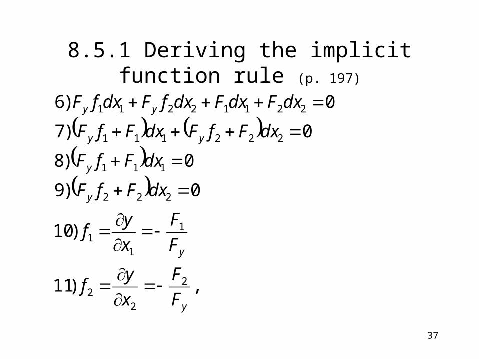
8.5.1 Deriving the implicit function rule (p. 197)
,)11
)10
0)9
0)8
0)7
0)6
2
22
1
11
222
111
222111
22112211
y
y
y
y
yy
yy
F
F
x
yf
F
F
x
yf
dxFfF
dxFfF
dxFfFdxFfF
dxFdxFdxfFdxfF
38
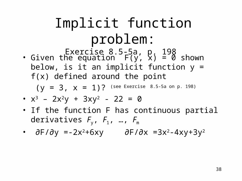
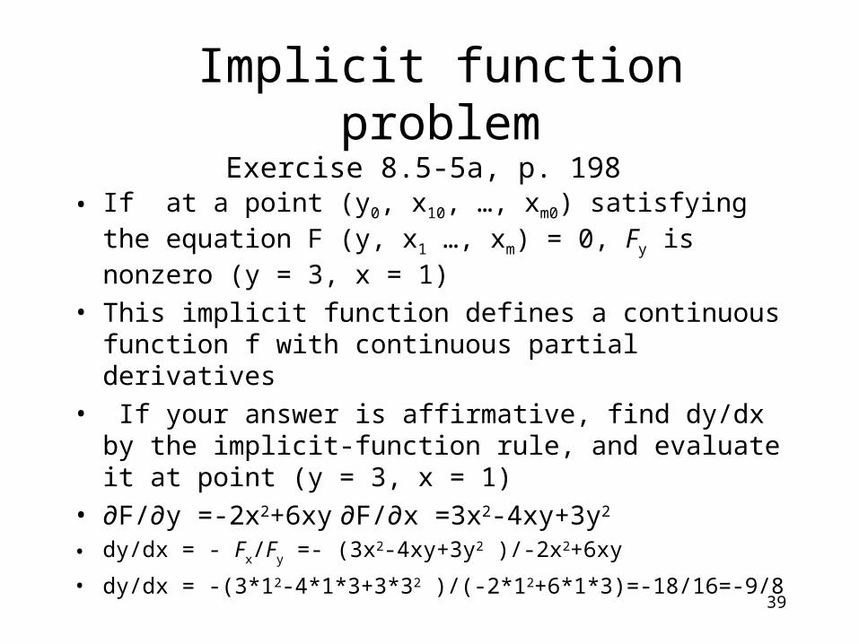
Implicit function problem:Exercise 8.5-5a, p. 198
• Given the equation F(y, x) = 0 shown below, is it an implicit function y = f(x) defined around the point (y = 3, x = 1)? (see Exercise 8.5-5a on p. 198)
• x3 – 2x2y + 3xy2 - 22 = 0• If the function F has continuous partial
derivatives Fy, F1, …, Fm
• ∂F/∂y =-2x2+6xy ∂F/∂x =3x2-4xy+3y2
39
Implicit function problemExercise 8.5-5a, p. 198
• If at a point (y0, x10, …, xm0) satisfying the equation F (y, x1 …, xm) = 0, Fy is nonzero (y = 3, x = 1)
• This implicit function defines a continuous function f with continuous partial derivatives
• If your answer is affirmative, find dy/dx by the implicit-function rule, and evaluate it at point (y = 3, x = 1)
• ∂F/∂y =-2x2+6xy ∂F/∂x =3x2-4xy+3y2 • dy/dx = - Fx/Fy =- (3x2-4xy+3y2 )/-2x2+6xy
• dy/dx = -(3*12-4*1*3+3*32 )/(-2*12+6*1*3)=-18/16=-9/8
40
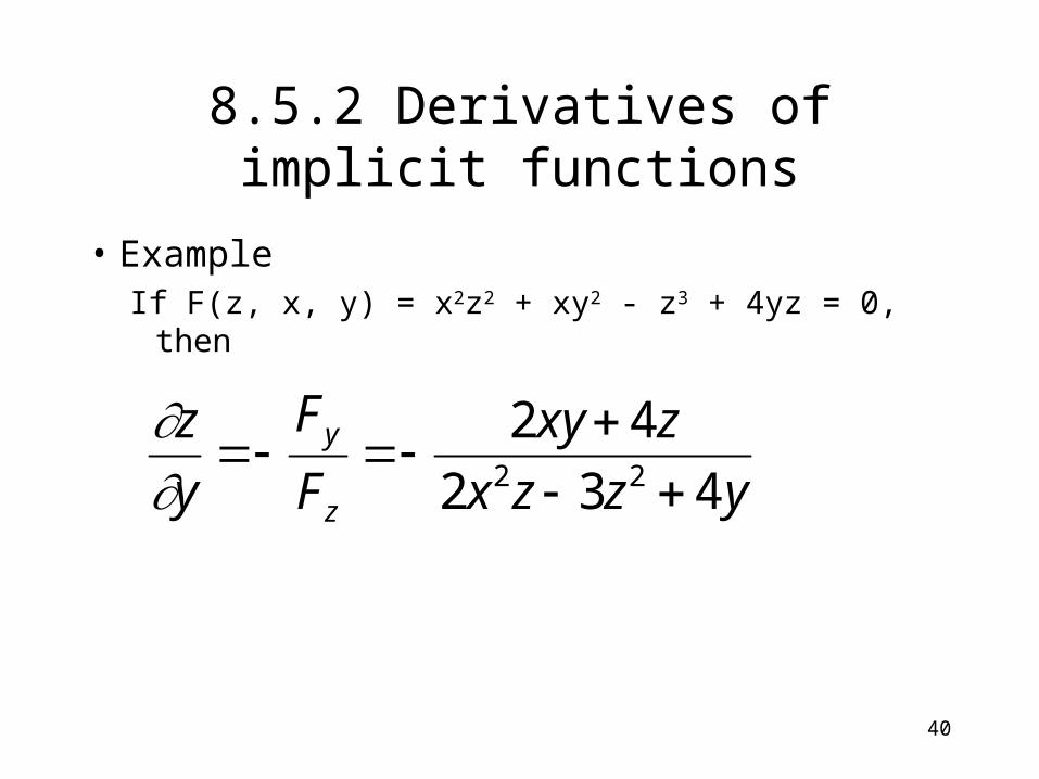
8.5.2 Derivatives of implicit functions
• ExampleIf F(z, x, y) = x2z2 + xy2 - z3 + 4yz = 0, then
yzzx
zxy
F
F
y
z
z
y
432
4222
41
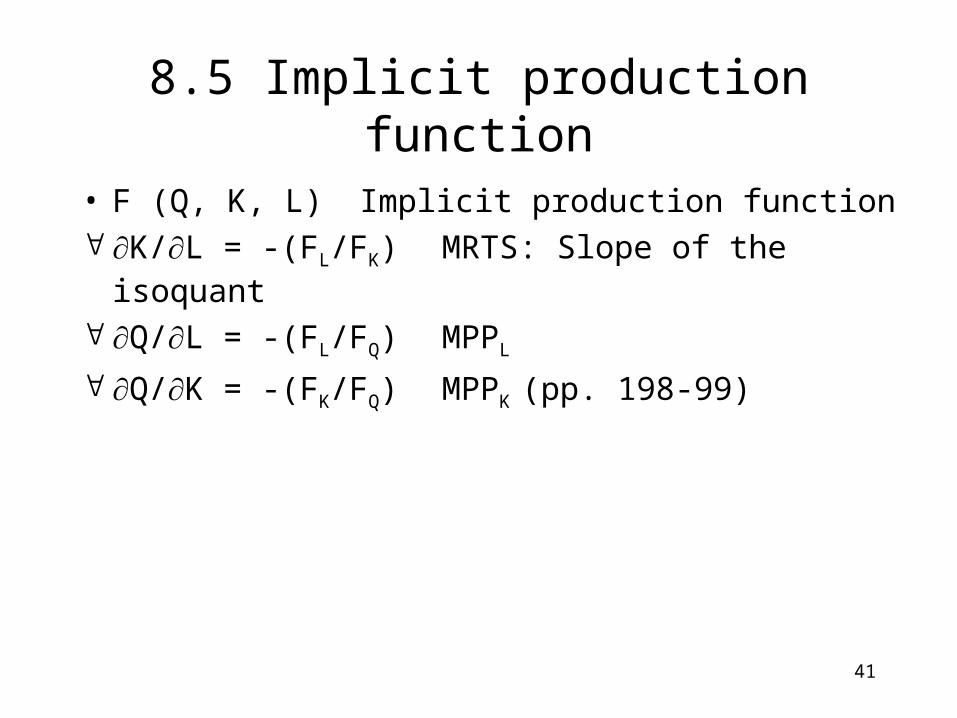
8.5 Implicit production function
• F (Q, K, L) Implicit production function K/L = -(FL/FK) MRTS: Slope of the isoquant
Q/L = -(FL/FQ) MPPL
Q/K = -(FK/FQ) MPPK (pp. 198-99)

42
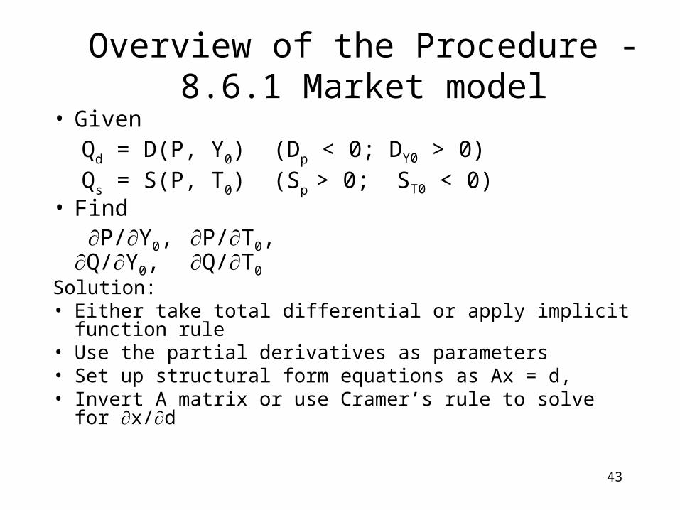
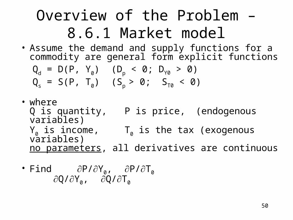
Overview of the Problem –8.6.1 Market model
• Assume the demand and supply functions for a commodity are general form explicit functionsQd = D(P, Y0) (Dp < 0; DY0 > 0)Qs = S(P, T0) (Sp > 0; ST0 < 0)
• where Q is quantity, P is price, (endogenous variables) Y0 is income, T0 is the tax (exogenous variables)no parameters, all derivatives are continuous
• Find P/Y0, P/T0 Q/Y0, Q/T0
43
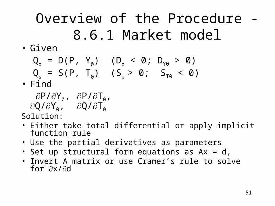
Overview of the Procedure -8.6.1 Market model
• GivenQd = D(P, Y0) (Dp < 0; DY0 > 0)Qs = S(P, T0) (Sp > 0; ST0 < 0)
• Find P/Y0, P/T0, Q/Y0, Q/T0
Solution: • Either take total differential or apply implicit function rule • Use the partial derivatives as parameters• Set up structural form equations as Ax = d, • Invert A matrix or use Cramer’s rule to solve for x/d
44
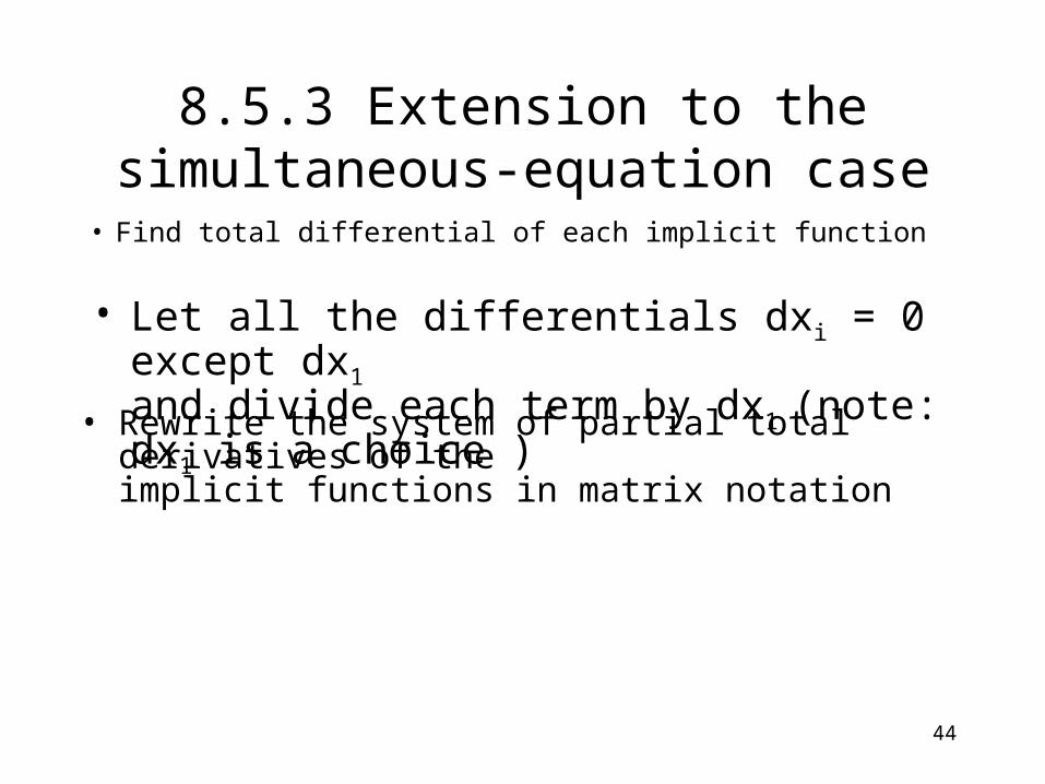
8.5.3 Extension to the simultaneous-equation case
• Find total differential of each implicit function
• Let all the differentials dxi = 0 except dx1
and divide each term by dx1 (note: dx1 is a choice )
• Rewrite the system of partial total derivatives of the implicit functions in matrix notation
45
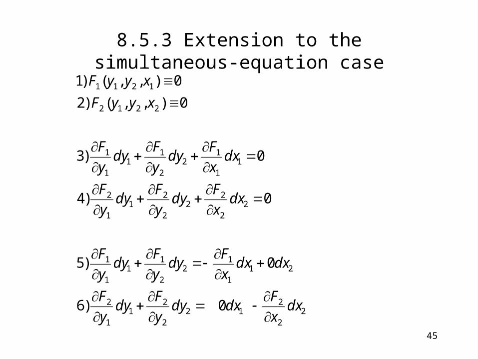
8.5.3 Extension to the simultaneous-equation case
22
212
2
21
1
2
211
12
2
11
1
1
22
22
2
21
1
2
11
12
2
11
1
1
2212
1211
0)6
0)5
0)4
0)3
0),,()2
0),,()1
dxx
Fdxdy
y
Fdy
y
F
dxdxx
Fdy
y
Fdy
y
F
dxx
Fdy
y
Fdy
y
F
dxx
Fdy
y
Fdy
y
F
xyyF
xyyF
46
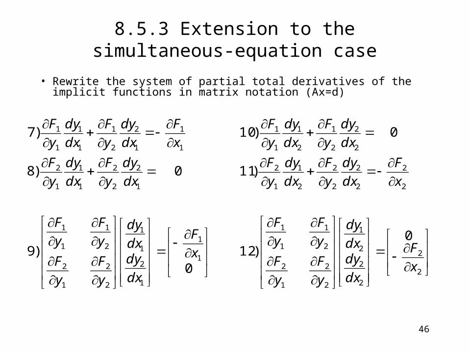
8.5.3 Extension to the simultaneous-equation case
• Rewrite the system of partial total derivatives of the implicit functions in matrix notation (Ax=d)
2
2
2
2
2
1
2
2
1
2
2
1
1
1
1
1
1
2
1
1
2
2
1
2
2
1
1
1
2
2
2
2
2
2
2
1
1
2
1
2
2
2
1
1
1
2
2
2
2
1
2
1
1
1
1
1
1
2
2
1
1
1
1
1
0)12
0)9
)110)8
0)10)7
x
F
dx
dydx
dy
y
F
y
F
y
F
y
F
x
F
dx
dydx
dy
y
F
y
F
y
F
y
F
x
F
dx
dy
y
F
dx
dy
y
F
dx
dy
y
F
dx
dy
y
F
dx
dy
y
F
dx
dy
y
F
x
F
dx
dy
y
F
dx
dy
y
F
47
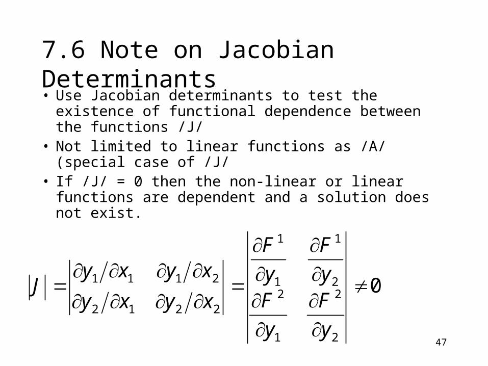
7.6 Note on Jacobian Determinants• Use Jacobian determinants to test the
existence of functional dependence between the functions /J/
• Not limited to linear functions as /A/ (special case of /J/
• If /J/ = 0 then the non-linear or linear functions are dependent and a solution does not exist.
0
2
2
1
22
1
1
1
2212
2111
y
F
y
Fy
F
y
F
xyxy
xyxyJ
48
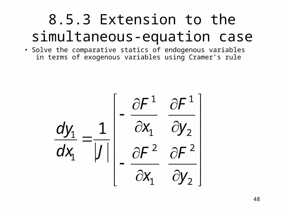
8.5.3 Extension to the simultaneous-equation case
• Solve the comparative statics of endogenous variables in terms of exogenous variables using Cramer’s rule
2
2
1
2
2
1
1
1
1
1 1
y
F
x
F
y
F
x
F
Jdx
dy
49
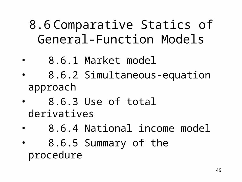
8.6 Comparative Statics of General-Function Models
• 8.6.1 Market model• 8.6.2 Simultaneous-equation
approach• 8.6.3 Use of total derivatives• 8.6.4 National income model• 8.6.5 Summary of the
procedure
50
Overview of the Problem –8.6.1 Market model
• Assume the demand and supply functions for a commodity are general form explicit functionsQd = D(P, Y0) (Dp < 0; DY0 > 0)Qs = S(P, T0) (Sp > 0; ST0 < 0)
• where Q is quantity, P is price, (endogenous variables) Y0 is income, T0 is the tax (exogenous variables)no parameters, all derivatives are continuous
• Find P/Y0, P/T0 Q/Y0, Q/T0
51
Overview of the Procedure -8.6.1 Market model
• GivenQd = D(P, Y0) (Dp < 0; DY0 > 0)Qs = S(P, T0) (Sp > 0; ST0 < 0)
• Find P/Y0, P/T0, Q/Y0, Q/T0
Solution: • Either take total differential or apply implicit function rule • Use the partial derivatives as parameters• Set up structural form equations as Ax = d, • Invert A matrix or use Cramer’s rule to solve for x/d
52
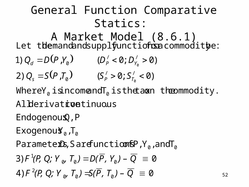
General Function Comparative Statics:
A Market Model (8.6.1)
0 )4
0 )3
T and ,Y P, of functions are S D, :Parameters
T,Y:Exogenous
P Q, :Endogenous
.continuous derivative All
commodity. on the tax theis T and income is Y Where
)0;0(,)2
)0;0(,)1
:becommodity afor functionssupply and demand Let the
0002
0001
00
00
00
//0
//0
0
0
Q) – , TPS(), T(P, Q; YF
Q) – , YPD(), T(P, Q; YF
SSTPSQ
DDYPDQ
TPs
YPd
53
General Function Comparative Statics: A Market Model
0//
0//
0//
0//
0*
0*
0*
0*
0
0
0
0
0
0
)8
)7
leftonvarsendog.onlyPut
0)6
0)5
;(4)&(3)equationsofaldifferentitotaltheTake
dTdP ,dYdP ,dTdQ ,dYdQ Find
0),()4
0),()3
dTSQdPdS
dYDQdPdD
QddTSPdS
QddYDPdD
QTPS
QYPD
TP
YP
TP
YP
54
General Function Comparative Statics: A Market Model
01
1)10
.det
0
0
1
1)9
);()8(&)7(
)8
)7
//
/
/
0
0
0/
/
/
/
0//
0//
0
0
0
PP
P
P
T
Y
P
P
TP
YP
DSS
DJ
JacobiantheofsigntheCalculate
dT
dY
S
D
Qd
Pd
S
D
dAxformatmatrixinequationsPut
dTSQdPdS
dYDQdPdD
55
General Function Comparative Statics: A Market Model
/
0
0/
/
/
0
0/
/
00
0
0
0/
/
/
/
0
0
0
0
1
1)13
01
1)12
dT var
)11(
0
0
1
1)11
TP
P
Y
P
P
T
Y
P
P
S
dT
QddT
Pd
S
D
D
dY
QddY
Pd
S
D
anddYsexogenouswrt
equationofsderivativetotalpartialtheTake
dT
dY
S
D
Qd
Pd
S
D
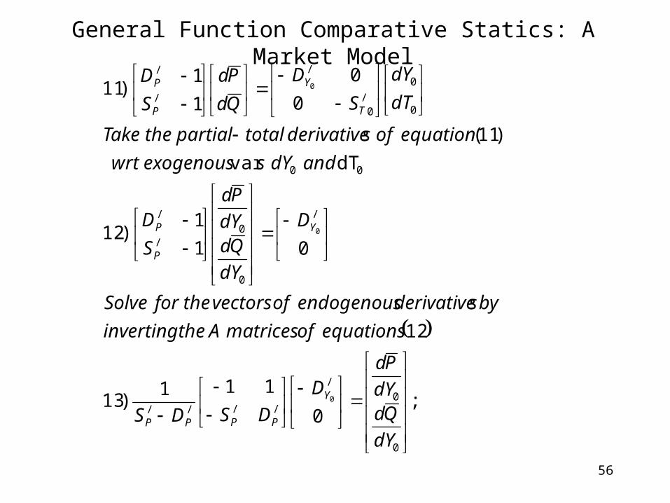
56
General Function Comparative Statics: A Market Model
;0
111)13
12
01
1)12
dT var
)11(
0
0
1
1)11
0
0/
////
/
0
0/
/
00
0
0
0/
/
/
/
0
0
0
dY
QddY
PdD
DSDS
equationsofmatricesAtheinverting
bysderivativeendogenousofvectorstheforSolve
D
dY
QddY
Pd
S
D
anddYsexogenouswrt
equationofsderivativetotalpartialtheTake
dT
dY
S
D
Qd
Pd
S
D
Y
PPPP
Y
P
P
T
Y
P
P
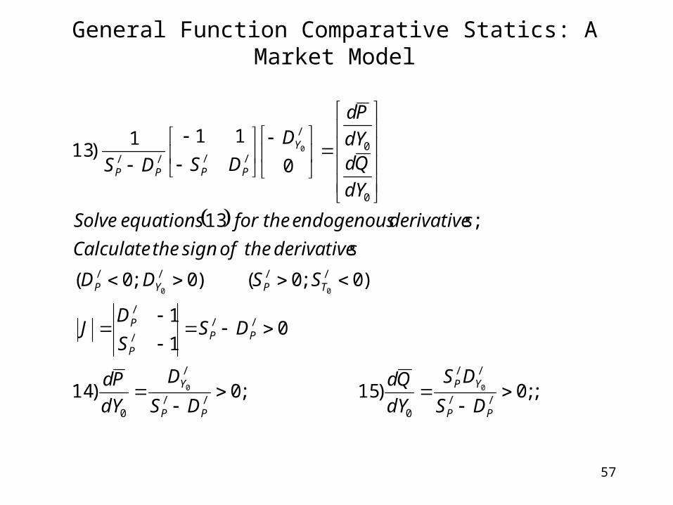
57
General Function Comparative Statics: A Market Model
;;0)15;0)14
01
1
)0;0()0;0(
;13
0
111)13
//
//
0//
/
0
//
/
/
////
0
0/
////
00
00
0
PP
YP
PP
Y
PP
P
P
TPYP
Y
PPPP
DS
DS
dY
Qd
DS
D
dY
Pd
DSS
DJ
SSDD
sderivativetheofsigntheCalculate
sderivativeendogenoustheforequationsSolve
dY
QddY
PdD
DSDS

58
General Function Comparative Statics: A Market Model
0)18;0)17
01
1
)0;0()0;0(
;16
0111)16
//
//
0//
/
0
//
/
/
////
0
0/////
00
00
0
PP
TP
PP
T
PP
P
P
TPYP
TPPPP
DS
SD
dT
Qd
DS
S
dT
Pd
DSS
DJ
SSDD
sderivativetheofsigntheCalculate
sderivativeendogenoustheforequationsSolve
dT
QddT
Pd
SDSDS
59
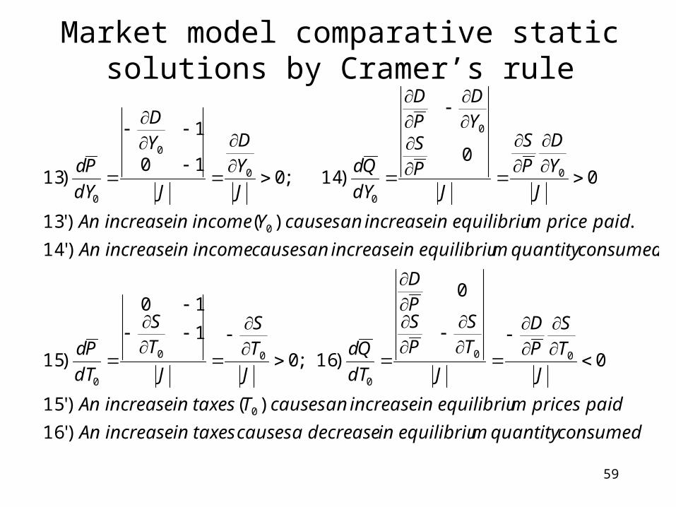
Market model comparative static solutions by Cramer’s rule
consumedquantitymequilibriuindecreaseacausestaxesinincreaseAn
paidpricesmequilibriuinincreaseancausesTtaxesinincreaseAn
J
TS
PD
J
TS
PSPD
dT
Qd
J
TS
J
TS
dT
Pd
consumedquantitymequilibriuinincreaseancausesincomeinincreaseAn
paidpricemequilibriuinincreaseancausesYincomeinincreaseAn
J
YD
PS
JPS
YD
PD
dY
Qd
J
YD
J
YD
dY
Pd
)'16
)()'15
0
0
)16;0
1
10
)15
.)'14
.)()'13
00
)14;010
1
)13
0
00
0
00
0
0
0
0
0
0
0
0
60
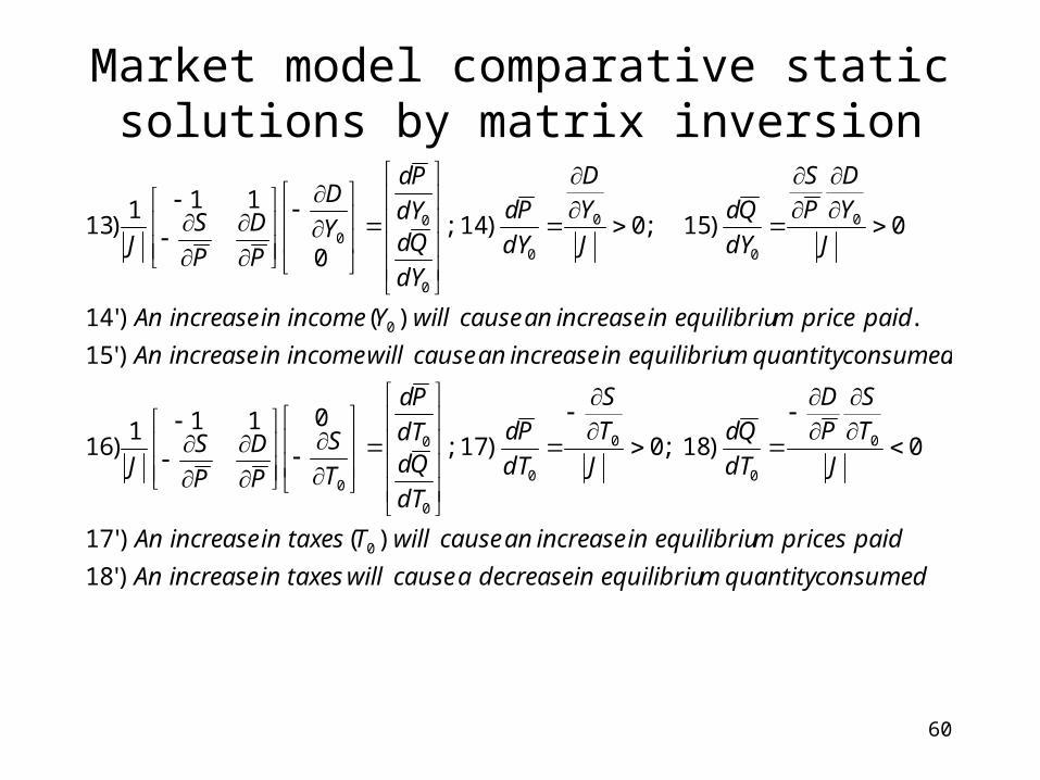
Market model comparative static solutions by matrix inversion
consumedquantitymequilibriuindecreaseacausewilltaxesinincreaseAn
paidpricesmequilibriuinincreaseancausewillTtaxesinincreaseAn
J
TS
PD
dT
Qd
J
TS
dT
Pd
dT
QddT
Pd
T
S
P
D
P
SJ
consumedquantitymequilibriuinincreaseancausewillincomeinincreaseAn
paidpricemequilibriuinincreaseancausewillYincomeinincreaseAn
J
YD
PS
dY
Qd
J
YD
dY
Pd
dY
QddY
Pd
Y
D
P
D
P
SJ
)'18
)()'17
0)18;0)17;0111
)16
.)'15
.)()'14
0)15;0)14;0
111)13
0
0
0
0
0
0
0
0
0
0
0
0
0
0
00
61
8.7 Limitations of Comparative Statics
• Comparative statics answers the question: how does the equilibrium change w/ a change in a parameter.
• The adjustment process is ignored
• New equilibrium may be unstable
• Before dynamic, optimization