CFD with OpenSource Software - Chalmershani/kurser/OS_CFD_2013/AbolfazlAsnagi/interP... · Asnaghi,...

Asnaghi, Shipping and Marine Technology, Chalmers University of Technology

CFD with OpenSource Software

A course at Chalmers University of Technology

Taught by Håkan Nilsson

interPhasChangeFoam Tutorial

and

PANS Turbulence Model

Developed for OpenFOAM-2.2.x

Author: Abolfazl Asnaghi

Peer reviewed by: Olivier Petit Tim Lackmann

Disclaimer: This is a student project work, done as part of a course where OpenFOAM and some

other OpenSource software are introduced to the students. Any reader should be aware that it

might not be free of errors. Still, it might be useful for someone who would like learn some

details similar to the ones presented in the report and in the accompanying les. The material has

gone through a review process. The role of the reviewer is to go through the tutorial and make

sure that it works, that it is possible to follow, and to some extent correct the writing. The

reviewer has no responsibility for the contents

Dec 2013


Preface

Current report contains descriptions of interPhaseChangeFoam solver and also detailed

explanation of adding a new turbulence model to OpenFoam code as the project report of

“MSc/PhD course in CFD with OpenSource software”. The OF2.2.x version has been used as the

default version for both of the cases.

In the first section of this report, interPhaseChangeFoam solver which has been used for

simulation of phase change between two incompressible-impressible flows has been described.

For phase change and as a default, different caviation phase change models have been considered

in this solver. Therefore, this solver has been used mostly for simulation of cavitation.

Previous students of this course have provided tutorial for this solver. Therefore, the emphasis of

this report would be on the sections which either need more explanation comparing to previous

tutorial or have been added/modified recently into the solver. Furthermore, in order to introduce

the way of modifying the solver, Singhal phase change model has been added to the solver, and

undertaken steps have been described.

It should be mentioned that it is assumed that the readers has gone through the lectures and

documents of the course, and therefore have some background on CFD/OpenFoam.

Finally, to show performance of the solver and its applicability, flows around two cases have

been simulated. The first case is the flow around a flat plate, and the second case is the flow

around a hydrofoil (NACA0009). At the end, few limitations and drawbacks of using this solver

have been discussed.

In the second section of the report, PANS turbulence model (Partially Averaged Navier Stokes)

has been presented. Numerical investigations of PANS turbulence models have shown their

merits and possible applicability to achieve high and precise results with lower computational

cost comparing to LES and DES approaches. Although there are still few unresolved problems

regarding stability of dynamic version of PANS models, promising results of these models have

caused its development especially in the cases that very fine mesh resolution is not possible due

to the lack of resources. For this tutorial, static version of PANS model based on the k-Epsilon

RANS model has been developed and implemented into the OpenFoam code. The

implementation is straightforward and can be easily extended to kOmega or other URANS

models. To verify the model and its superiority over original URANS model (here kEpsilon),

turbulent flow around a square cylinder has been simulated. To give a wider view, K-Epsilon,


OEEVM, and PANS k-Epsilon models have been compared and merits of the implemented

model over other models are verified.


Contents

Figure List ....................................................................................................................................... 5

Table List ........................................................................................................................................ 5

1. First Section: interPhaseChangeFoam ........................................................................................ 6

1.1 Introduction ........................................................................................................................... 6

1.2 Governing equations ............................................................................................................. 6

1.3 Solver members .................................................................................................................... 8

1.3.1 SchnerrSauer.C .............................................................................................................. 9

1.3.2 phaseChangeTwoPhaseMixture.C ............................................................................... 12

1.3.3 alphaEqn.H................................................................................................................... 13

1.3.4 alphaEqnSubCycle.H ................................................................................................... 15

1.3.5 pEqn.H ......................................................................................................................... 15

1.4 Modifications ...................................................................................................................... 16

1.4.1 alphaEqn.H................................................................................................................... 16

14.2 Negative pressure .......................................................................................................... 16

1.5 Test case: flow behind a flat plate....................................................................................... 16

2. Second Section: PANS ............................................................................................................. 19

2.1 Introduction ......................................................................................................................... 19

2.2 Background ......................................................................................................................... 19

2.3 Theory ................................................................................................................................. 20

2.4 Implementation into OpenFoam2.2x .................................................................................. 22

2.4.1 kEpsilonPANS.C ......................................................................................................... 22

2.4.2 kEpsilonPANS.H ......................................................................................................... 25

2.5 Results ................................................................................................................................. 26

2.6 Post processing.................................................................................................................... 27


3. References ................................................................................................................................. 31

Figure List

Figure (1-1) – Geometry and boundary conditions for simulation cavitation in 2d flat plate ...... 17

Figure (1-2) – one snapshot of cavitation and velocity vectors around the flat plate ................... 17

Figure (1-3) – Average drag coefficient of the 2d flat plate for cavitation number equal to one,

Experiments [8] ............................................................................................................................. 18

Figure (2-1) –Square cylinder mesh structure .............................................................................. 26

Table List

Table (2-1) – Comparing different turbulence models results for flow around the square cylinder,

Re=22e3, inlet velocity 0.54 m/s with 2% turbulence fluctuation ................................................ 27


1. First Section: interPhaseChangeFoam

1.1 Introduction

To simulate cavitating flows with OpenFoam code, there are few solvers available which have

been designed for simulating this type of fluids. One of these solvers is interPhaseChangeFoam

which has been especially written for incompressible/immiscible two phase flows. This solver in

the version of 2.2.x is located in OpenFoam/applications/solvers/multiphase. In the recently

released version of the code (OF2.2.2), interDyPhaseChangeFoam has been added to simulate

cavitation around moving objects like propellers.

In the following parts of the first section, first of all governing equations of two phase

incompressible flows are represented. Then all of the members of the solver are listed and for

those which we have more concerns all of the code parts have been described and explained.

The case folder for this solver like most of the solvers consists of three folders: time (zero),

constant, and system.

In the system folder, you have to define solution parameters (fvSolution file), schemes

(fvSchemes) and also time parameters (controlDict). In the constant folder, you have to define

the solver parameters like phase change model and its characteristics through transportProperties

file.

There is a tutorial for this solver where you can find a template and example of how to set these

parameters which is located at

“$WM_PROJECT_DIR/tutorials/multiphase/interPhaseChangeFoam”

In the following, governing equations, solver members list, solver members descriptions, results

for a test case, and some issues regarding the drawbacks of simulation of cavitation have been

presented.

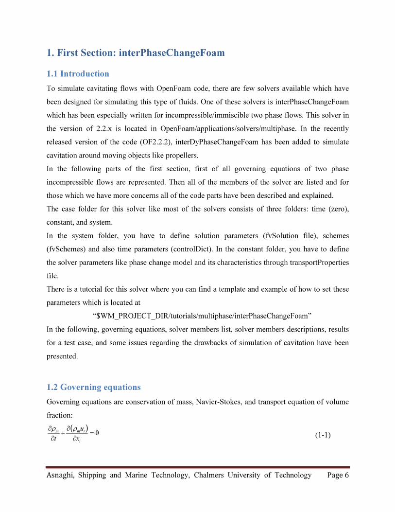
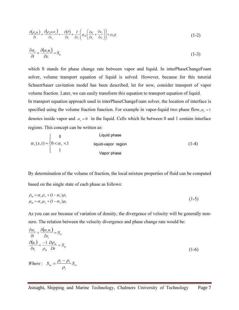
1.2 Governing equations

Governing equations are conservation of mass, Navier-Stokes, and transport equation of volume

fraction:

(1-1) ( )

0=∂

∂+

∂

∂

i

imm

x

u

t

ρρ


(1-2) ( ) ( ) ( )

gx

u

x

u

xx

P

x

uu

t

um

i

j

j

i

eff

jij

jimimρµ

ρρ+

∂

∂+

∂

∂

∂

∂+

∂

∂−=

∂

∂+

∂

∂

(1-3) ( )

α

αα

Sx

u

ti

ivv=

∂

∂+

∂

∂

which S stands for phase change rate between vapor and liquid. In interPhaseChangeFoam

solver, volume transport equation of liquid is solved. However, because for this tutorial

SchnerrSauer cavitation model has been described, let for now, consider transport of vapor

volume fraction. Later, we can easily transform this equation to transport equation of liquid.

In transport equation approach used in interPhaseChangeFoam solver, the location of interface is

specified using the volume fraction function. For example in vapor-liquid two phase flow, 1=vα

denotes inside vapor and 0=vα in the liquid. Cells which lie between 0 and 1 contain interface

regions. This concept can be written as:

(1-4)

Liquid phase

<<=

1

10

0

),(vv

tx αα liquid-vapor region

Vapor phase

By determination of the volume of fraction, the local mixture properties of fluid can be computed

based on the single state of each phase as follows:

(1-5) lvvvm

lvvvm

µαµαµ

ραραρ

)1(

)1(

−+=

−+=

As you can see because of variation of density, the divergence of velocity will be generally non-

zero. The relation between the velocity divergence and phase change rate would be:

(1-6)

( )

( )m

m

mi

i

i

ivv

SDt

D

x

u

Sx

u

t

=−

=∂

∂

=∂

∂+

∂

∂

ρ

ρ

αα

α

1

α

ρ

ρρSSWhere

l

vl

m

−

=:


1.3 Solver members

This solver consists of the following files/folders.

o alphaEqn.H

o alphaEqnSubCycle.H

o createFields.H

o interPhaseChangeFoam.C

o pEqn.H

o UEqn.H

o phaseChangeTwoPhaseMixtures Folder

• Kunz folder

� Kunz.C

� Kunz.H

• Merkle folder

� Merkle.C

� Merkle.H

• phaseChangeTwoPhaseMixture

� phaseChangeTwoPhaseMixture.C

� phaseChangeTwoPhaseMixture.H

� newPhaseChangeTwoPhaseMixture.C

� newPhaseChangeTwoPhaseMixture.H

• SchnerrSauer folder

� SchnerrSauer.C

� SchnerrSauer.H

o Make

• files

• options

Here, we have focused on those files which are more specific for this solver. The solver is

located at

“$WM_PROJECT_DIR/applications/solvers/multiphase/interPhaseChangeFoam”


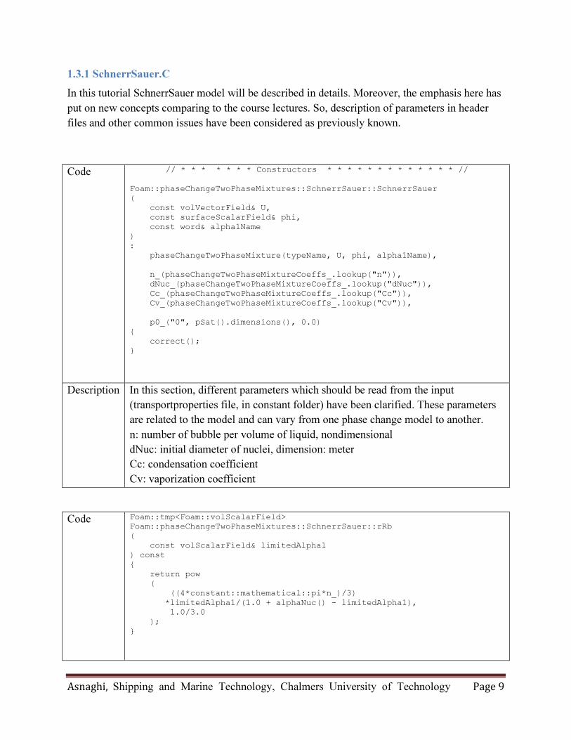
1.3.1 SchnerrSauer.C

In this tutorial SchnerrSauer model will be described in details. Moreover, the emphasis here has

put on new concepts comparing to the course lectures. So, description of parameters in header

files and other common issues have been considered as previously known.

Code // * * * * * * * Constructors * * * * * * * * * * * * * // Foam::phaseChangeTwoPhaseMixtures::SchnerrSauer::SchnerrSauer ( const volVectorField& U, const surfaceScalarField& phi, const word& alpha1Name ) : phaseChangeTwoPhaseMixture(typeName, U, phi, alpha1Name), n_(phaseChangeTwoPhaseMixtureCoeffs_.lookup("n")), dNuc_(phaseChangeTwoPhaseMixtureCoeffs_.lookup("dNuc")), Cc_(phaseChangeTwoPhaseMixtureCoeffs_.lookup("Cc")), Cv_(phaseChangeTwoPhaseMixtureCoeffs_.lookup("Cv")), p0_("0", pSat().dimensions(), 0.0) { correct(); }

Description In this section, different parameters which should be read from the input

(transportproperties file, in constant folder) have been clarified. These parameters

are related to the model and can vary from one phase change model to another.

n: number of bubble per volume of liquid, nondimensional

dNuc: initial diameter of nuclei, dimension: meter

Cc: condensation coefficient

Cv: vaporization coefficient

Code Foam::tmp<Foam::volScalarField> Foam::phaseChangeTwoPhaseMixtures::SchnerrSauer::rRb ( const volScalarField& limitedAlpha1 ) const { return pow ( ((4*constant::mathematical::pi*n_)/3) *limitedAlpha1/(1.0 + alphaNuc() - limitedAlpha1), 1.0/3.0 ); }


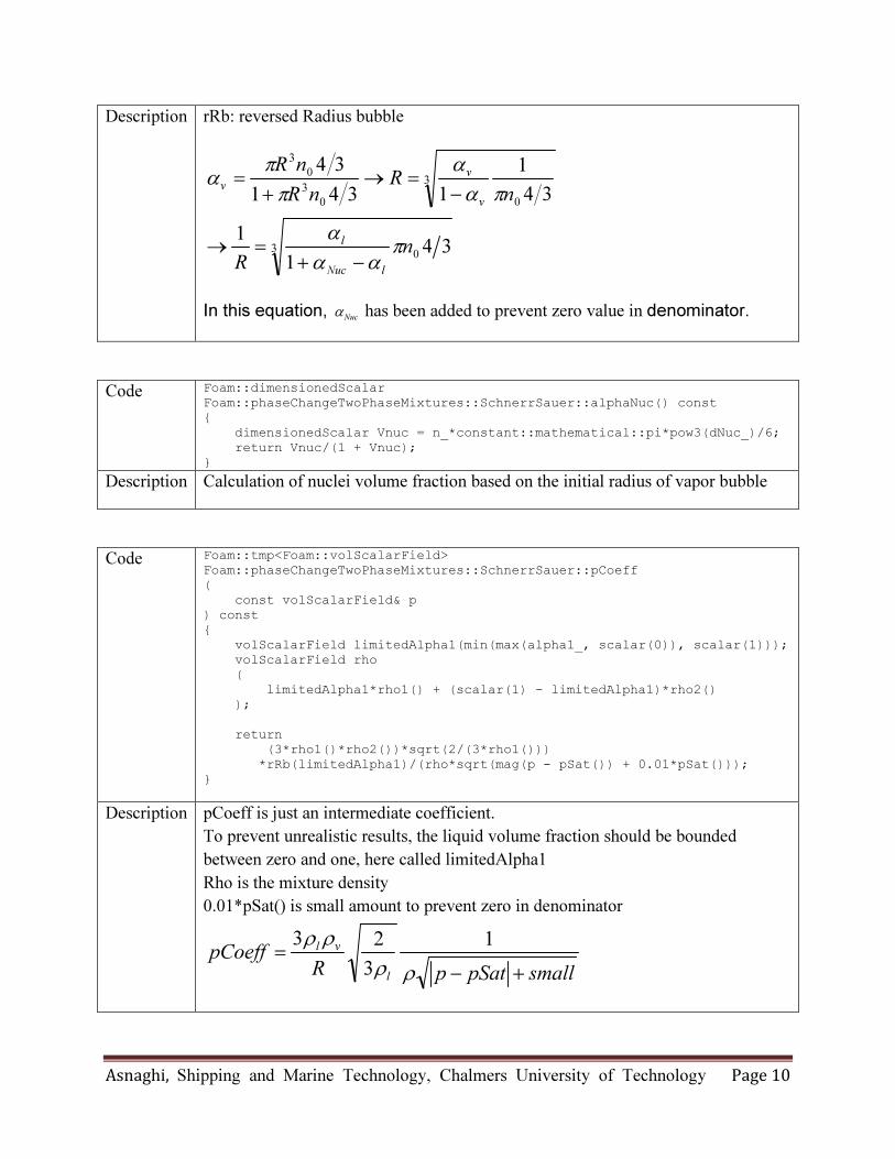
Description rRb: reversed Radius bubble

30

3

00

3

0

3

341

1

34

1

1341

34

nR

nR

nR

nR

lNuc

l

v

v

v

π

αα

α

πα

α

π

π

α

−+

=→

−

=→

+

=

In this equation, Nucα has been added to prevent zero value in denominator.

Code Foam::dimensionedScalar Foam::phaseChangeTwoPhaseMixtures::SchnerrSauer::alphaNuc() const { dimensionedScalar Vnuc = n_*constant::mathematical::pi*pow3(dNuc_)/6; return Vnuc/(1 + Vnuc); }

Description Calculation of nuclei volume fraction based on the initial radius of vapor bubble

Code Foam::tmp<Foam::volScalarField> Foam::phaseChangeTwoPhaseMixtures::SchnerrSauer::pCoeff ( const volScalarField& p ) const { volScalarField limitedAlpha1(min(max(alpha1_, scalar(0)), scalar(1))); volScalarField rho ( limitedAlpha1*rho1() + (scalar(1) - limitedAlpha1)*rho2() ); return (3*rho1()*rho2())*sqrt(2/(3*rho1())) *rRb(limitedAlpha1)/(rho*sqrt(mag(p - pSat()) + 0.01*pSat())); }

Description pCoeff is just an intermediate coefficient.

To prevent unrealistic results, the liquid volume fraction should be bounded

between zero and one, here called limitedAlpha1

Rho is the mixture density

0.01*pSat() is small amount to prevent zero in denominator

smallpSatpRpCoeff

l

vl

+−

=

ρρ

ρρ 1

3

23


Code Foam::Pair<Foam::tmp<Foam::volScalarField> > Foam::phaseChangeTwoPhaseMixtures::SchnerrSauer::mDotAlphal() const { const volScalarField& p = alpha1_.db().lookupObject<volScalarField>("p"); volScalarField limitedAlpha1(min(max(alpha1_, scalar(0)), scalar(1))); volScalarField pCoeff(this->pCoeff(p)); return Pair<tmp<volScalarField> > ( Cc_*limitedAlpha1*pCoeff*max(p - pSat(), p0_), Cv_*(1.0 + alphaNuc() - limitedAlpha1)*pCoeff*min(p - pSat(), p0_) ); }

Description mDotAlphal is a pair volScalarField. The first part is related to condensation, and

the second is related to evaporation. Pressure is loaded into this section by

lookupObject.

mDotAlphal will be used in transport equation of liquid volume fraction.

Code Foam::Pair<Foam::tmp<Foam::volScalarField> > Foam::phaseChangeTwoPhaseMixtures::SchnerrSauer::mDotP() const { const volScalarField& p = alpha1_.db().lookupObject<volScalarField>("p"); volScalarField limitedAlpha1(min(max(alpha1_, scalar(0)), scalar(1))); volScalarField apCoeff(limitedAlpha1*pCoeff(p)); return Pair<tmp<volScalarField> > ( Cc_*(1.0 - limitedAlpha1)*pos(p - pSat())*apCoeff, (-Cv_)*(1.0 + alphaNuc() - limitedAlpha1)*neg(p - pSat())*apCoeff ); }

Description mDotP is a pair volScalarField. The first part is related to condensation, and the

second is related to evaporation. Pressure is loaded into this section by

lookupObject.

Code bool Foam::phaseChangeTwoPhaseMixtures::SchnerrSauer::read() { if (phaseChangeTwoPhaseMixture::read()) { phaseChangeTwoPhaseMixtureCoeffs_ = subDict(type() + "Coeffs"); phaseChangeTwoPhaseMixtureCoeffs_.lookup("n") >> n_; phaseChangeTwoPhaseMixtureCoeffs_.lookup("dNuc") >> dNuc_; phaseChangeTwoPhaseMixtureCoeffs_.lookup("Cc") >> Cc_;


phaseChangeTwoPhaseMixtureCoeffs_.lookup("Cv") >> Cv_; return true; } else { return false; } }

Description Reading model parameters from input (constant/transportProperties)

1.3.2 phaseChangeTwoPhaseMixture.C

Code Foam::Pair<Foam::tmp<Foam::volScalarField> > Foam::phaseChangeTwoPhaseMixture::vDotAlphal() const { volScalarField alphalCoeff(1.0/rho1() - alpha1_*(1.0/rho1() - 1.0/rho2())); Pair<tmp<volScalarField> > mDotAlphal = this->mDotAlphal(); return Pair<tmp<volScalarField> > ( alphalCoeff*mDotAlphal[0], alphalCoeff*mDotAlphal[1] ); }

Description vDotAlphal which consists of two parts defined as follow:

−−=

valphaLmDotAlphaLvDotAlphaL

llρρρ

11.

1.

Code Foam::Pair<Foam::tmp<Foam::volScalarField> > Foam::phaseChangeTwoPhaseMixture::vDotP() const { dimensionedScalar pCoeff(1.0/rho1() - 1.0/rho2()); Pair<tmp<volScalarField> > mDotP = this->mDotP(); return Pair<tmp<volScalarField> >(pCoeff*mDotP[0], pCoeff*mDotP[1]); }

Description

−=

vmDotpvDotp

lρρ

11.

Code bool Foam::phaseChangeTwoPhaseMixture::read() { if (incompressibleTwoPhaseMixture::read()) { phaseChangeTwoPhaseMixtureCoeffs_ = subDict(type() + "Coeffs"); lookup("pSat") >> pSat_;


return true; } else { return false; } }

Description Looking up for coefficients and pSat

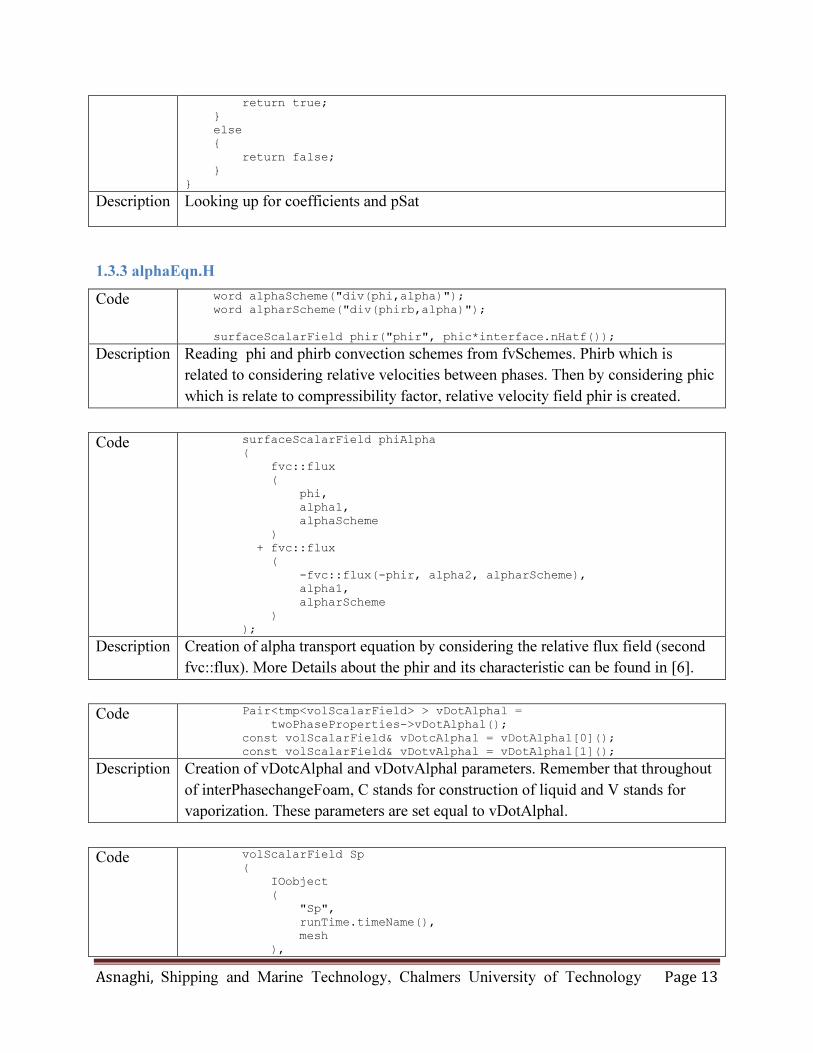
1.3.3 alphaEqn.H

Code word alphaScheme("div(phi,alpha)"); word alpharScheme("div(phirb,alpha)"); surfaceScalarField phir("phir", phic*interface.nHatf());

Description Reading phi and phirb convection schemes from fvSchemes. Phirb which is

related to considering relative velocities between phases. Then by considering phic

which is relate to compressibility factor, relative velocity field phir is created.

Code surfaceScalarField phiAlpha ( fvc::flux ( phi, alpha1, alphaScheme ) + fvc::flux ( -fvc::flux(-phir, alpha2, alpharScheme), alpha1, alpharScheme ) );

Description Creation of alpha transport equation by considering the relative flux field (second

fvc::flux). More Details about the phir and its characteristic can be found in [6].

Code Pair<tmp<volScalarField> > vDotAlphal = twoPhaseProperties->vDotAlphal(); const volScalarField& vDotcAlphal = vDotAlphal[0](); const volScalarField& vDotvAlphal = vDotAlphal[1]();

Description Creation of vDotcAlphal and vDotvAlphal parameters. Remember that throughout

of interPhasechangeFoam, C stands for construction of liquid and V stands for

vaporization. These parameters are set equal to vDotAlphal.

Code volScalarField Sp ( IOobject ( "Sp", runTime.timeName(), mesh ),


vDotvAlphal - vDotcAlphal ); volScalarField Su ( IOobject ( "Su", runTime.timeName(), mesh ), // Divergence term is handled explicitly to be // consistent with the explicit transport solution divU*alpha1 + vDotcAlphal );

Description Creation of Sp and Su for MULES solver.

al vDotcAlph+alpha1*divUSu

al vDotcAlph- lvDotvAlpha

=

=Sp

Code MULES::implicitSolve ( geometricOneField(), alpha1, phi, phiAlpha, Sp, Su, 1, 0 );

Description Solving the alpha equation by using MULES solver. Please take a look at NaiXian

Lu report for this course, 2008.

Code MULES::implicitSolve ( geometricOneField(), alpha1, phi, phiAlpha, Sp, Su, 1, 0 );

Description Solving the alpha equation by using MULES solver.

Please take a look at NaiXian Lu report for this course [7].

I strongly suggest that you add a bounding for alpha after solving the transport

equation to prevent from non-physical values.


1.3.4 alphaEqnSubCycle.H

Code surfaceScalarField rhoPhi ( IOobject ( "rhoPhi", runTime.timeName(), mesh ), mesh, dimensionedScalar("0", dimMass/dimTime, 0) );

Description Creation of surface scalar field for rhoPhi: mass flux

Code const dictionary& pimpleDict = pimple.dict(); label nAlphaCorr(readLabel(pimpleDict.lookup("nAlphaCorr"))); label nAlphaSubCycles(readLabel(pimpleDict.lookup("nAlphaSubCycles")));

Description Looking up to the pimple dictionary to read values of nAlphaSubCycles,

nAlphaCorr

1.3.5 pEqn.H

Code Pair<tmp<volScalarField> > vDotP = twoPhaseProperties->vDotP(); const volScalarField& vDotcP = vDotP[0](); const volScalarField& vDotvP = vDotP[1](); while (pimple.correctNonOrthogonal()) { fvScalarMatrix p_rghEqn ( fvc::div(phiHbyA) - fvm::laplacian(rAUf, p_rgh) - (vDotvP - vDotcP)*(pSat - rho*gh) + fvm::Sp(vDotvP - vDotcP, p_rgh) ); } }

Description Loading vDotP parameters as vDotcP and vDotvP.

Since we solve for p_rgh which is equal to p- rho*gh, we have to reduce the

hydrostatic pressure from pSat too: pSat - rho*gh


1.4 Modifications

1.4.1 alphaEqn.H

Although the MULES solver was developed to solve the equation of bounded variables;

sometimes it fails to keep the variable in its bounds. Therefore, in order to prevent unrealistic

values for alpha (i.e. values higher than one or lowers than zero); in alphaEqn.H the following

command line has been added after the MULES solver.

alpha1 = min(max(alpha1, scalar(0)), scalar(1));

14.2 Negative pressure

Depending on the flow conditions, in some cases the minimum pressure value may go below the

zero by using default values for number of nuclei, nuclei diameter, and coefficients. To prevent

from this unrealistic condition, one option is using a very high value for evaporation coefficient

(Cv around 5000). Another approach would be using a high value for number of nuclei (n0

around 1e14). It should be considered that alphaNuc should always have reasonable value

(around 1e-5). Therefore, in the case of using high value for n0, the diameter of nuclei should be

set according the reasonable value of alphaNuc.

Because the pressure values through solution have high importance, it may be necessary to watch

the pressure values during solution. Therefore, at the end of “interPhaseChangeFoam.C” file, and

inside the time loop add the following simple command.

Info << "Max pressure: " << max(p).value() << endl; Info << "Min pressure: " << min(p).value() << endl; Info << "Max velocity: " << max(mag(U)).value() << endl << endl;

1.5 Test case: flow behind a flat plate

Flow around a 2d flat plate has been simulated using the interPhaseChangeFoam solver. The

inlet velocity is 5 m/s, and outlet cavitation number is set equal to one. The height of the plat is

0.1 m and its thickness is 0.01 m. The experimental data for this case have been derived from [8].

In the Figure (1-1), geometry and boundary conditions have been presented. As it can be seen,

the inlet condition is velocity constant and outlet condition is pressure constant. H is the height


of the plate. In Figure (1-2), one snap shot of flow around the plate is depicted. This picture

shows the interaction between the vapor phases and velocity field.

Figure (1-1) – Geometry and boundary conditions for simulation cavitation in 2d flat plate

Figure (1-2) – one snapshot of cavitation and velocity vectors around the flat plate

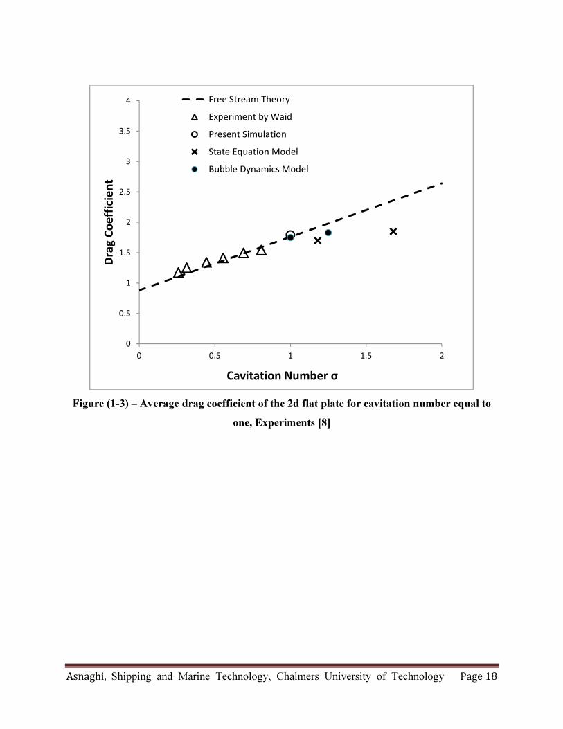
To validate the current simulation with experimental data, in Figure (1-3), variations of drag

coefficient by cavitation number is presented. As it can be seen, the comparison shows the

accuracy of the performed simulation. To obtain the drag coefficients, openFoam library has

been used. More details about post processing and data gathering have been provided in section

(2.6) of this report.


Figure (1-3) – Average drag coefficient of the 2d flat plate for cavitation number equal to

one, Experiments [8]

0

0.5

1

1.5

2

2.5

3

3.5

4

0 0.5 1 1.5 2

Dra

g C

oe

ffic

ien

t

Cavitation Number σ

Free Stream Theory

Experiment by Waid

Present Simulation

State Equation Model

Bubble Dynamics Model


2. Second Section: PANS

2.1 Introduction

Different turbulence models have different levels of accuracy in predicting Reynolds Stress

Tensors depending on their time or space turbulence spectrum cut off size. However, there are

usually limitations in selecting turbulence models based on the computational utilities, or in

simple words affordable computational cost. Among the different turbulence models categories,

the following models are more famous and have been used wider both in academic and industrial

applications:

• RANS (Reynolds Averaged Navier Stokes)

• LES (Large Eddy Simulation)

• DES (Detached Eddy Simulation)

• DNS (Direct Numerical Simulation) – less used in industry because of huge amount of

computational cost

• Hybrid method: combining the above mentioned turbulence models to get more efficient

models, e.g. PANS

There are a lot of papers describing these models and their applications which one can easily find

more information about these models. Generally speaking, it is hard to say which one of these

models is more appropriate than the others for a specified case.

In the following, PANS turbulence model has been described, and then added to OpenFoam

Turbulence Library. Finally, for well-known benchmark (flow over a square cylinder) numerical

results of this model has been compared with other available turbulence models in OpenFoam.

2.2 Background

RANS turbulence models use averaged velocity as the velocity appears in Navier-Stokes

equations. This averaged velocity is calculated by averaging over all velocity disturbance

spectrums in cut-off size (grid size). Although this approach will lead to an increase in speed of

calculation, because of averaging all velocity disturbance (which some of them can have

important energy content) it will cause in a lack of accuracy.

Another option would be to use DNS. This approach considers all of the velocity disturbance

spectrums during calculation of turbulence stress tensor. Therefore, this model will guarantee a

higher precision in solution. The main disadvantage of DNS is its CPU cost. Because in solving


procedure, all of the velocity disturbance spectrums have been considered (which some of them

may be not so important) the computational cost of this approach is very high, and is the major

barrier (currently!) in its development.

PANS stands for ‘Partially Averaged Navier Stockes”, and the idea of this method is to average

some portion of velocity disturbance spectrums. Therefore, it would be placed between RANS

and DNS.

PANS

RANS

DNS

Averaging all velocity

disturbance spectrums

Solving all velocity

disturbance spectrums

Lower CPU cost Higher CPU cost

It should be mentioned that the part of velocity disturbance spectrums that is averaged is called

unresolved part because we do not solve it directly. Effects of unresolved part are considered by

modeling, i.e. the turbulence model will handle that!

So, Partially Averaged Navier-Stokes (PANS) turbulence method provides a closure model for

any degree of velocity filtering - ranging from completely resolved Direct Numerical Simulation

(DNS) to completely averaged Reynolds Averaged Navier-Stokes (RANS) method. Preliminary

investigations of PANS show promising results but there still exist computational and physical

issues that must be addressed.

2.3 Theory

The PANS bridging method [2] provides a smooth transition from DNS to RANS based upon a

user specified filter parameter. The flow field is decomposed into resolved and residual terms

(unresolved) as opposed to the mean and fluctuating terms of RANS methodology. It is expected

that a PANS simulation can be more accurate as key fluctuations are considered in its resolved

part of the flow. The difference between PANS and LES methodologies is that PANS is


purposed for resolving significantly lesser number of scales. The control parameters of the PANS

model are resolved-to-unresolved kinetic energy and resolved-to-unresolved dissipation. The

closure equations are developed in a manner similar to the RANS model equations for an

arbitrary filter. Therefore, the PANS model is derived systematically from corresponding parent

RANS models. In this study, the parent RANS models used for simulations are kEpsilon. So, let

start from standard version of kEpsilon model [3]:

For turbulent kinetic energy K

(2-1) ( ) ( )

ρεσ

µµ

ρρ−+

∂

∂

+

∂

∂=

∂

∂+

∂

∂k

ik

t

ii

immP

x

k

xx

ku

t

k

For dissipation ε

(2-2) ( ) ( )

( )εεεε

ε

ερ

εε

σ

µµ

ερερS

kCPCP

kC

xxx

u

tbk

i

t

ii

imm +−++

∂

∂

+

∂

∂=

∂

∂+

∂

∂ 2

231

Turbulent viscosity is modeled as:

(2-3) ε

ρµµ

2k

Ct=

Production of k:

(2-4) 2Sp

tµ=

Model Constants:

(2-5) 3.1,0.1,09.0,33.0,92.1,44.1321

===−===εµεεεσσ

kCCCC

By decomposing the velocity field into the resolved and unresolved parts, and also by

introducing fK, and fEpsilon as the ratio of unresolved to resolved values, these equations can be

mapped into the PANS model. Few assumptions should be considered in order to simplify these

equations which have been discussed in literatures [4, 5].

The final equations governing PANS turbulence model are as follows (remember for parent

RANS kEpsilon):

(2-6) ( ) ( )

uu

i

u

ku

u

ii

uimumP

x

k

xx

ku

t

kρε

σ

µµ

ρρ−+

∂

∂

+

∂

∂=

∂

∂+

∂

∂


(2-7) ( ) ( )

εεε

ε

ερ

εε

σ

µµ

ερερS

kC

k

PCf

xxx

u

tu

u

u

uu

k

i

u

u

u

ii

uimum +

−+

∂

∂

+

∂

∂=

∂

∂+

∂

∂2

*

21

(2-8) u

u

ut

kC

ερµ

µ

2

=

(2-9) ε

ε

ε

uu

kf

K

Kf == ,

(2-10) ( )ε

εε

ε

εεσσ

f

fCC

f

fCC k

u

k

2

121

*

2, =−+=

As you can see, the shape of the equations are the same, and therefore relatively easy

modification would be required to create this new turbulence model from the already exist

kEpsilon model in OpenFoam.

2.4 Implementation into OpenFoam2.2x

Here is the procedure to create PANS turbulence model from original kEpsilon model in OF22x:

1- Open a new terminal

2- Load openfoam

3- Copy kEpsilon turbulence model to your directory

4- Rename the folder and its files (kEpsilon.C and kEpsilon.H) to kEpsilonPANS

5- Replace kEpsilon with kEpsilonPANS in .C and .H files

6- Go to Make folder, and then into the files

7- Replace kEpsilon with kEpsilonPANS, and also libkEpsilon with libkEpsilonPANS

8- Complete description of these procedures are presented in the course, and at the section

related to adding a new turbulence model. From now, PANS related modifications have

been presented in more details:

2.4.1 kEpsilonPANS.C

o It is necessary to read some information from the input regarding the PANS coefficients

(RASproperties file, and in the kEpsilonPANS dictionary). So, in the Constructors part of

kEpsilonPANS.C, and between definitions of sigmaEps_ and k_, define the following

parameters: fEpsilon, and fK

fEpsilon_

(

dimensioned<scalar>::lookupOrAddToDict


(

"fEpsilon",

coeffDict_,

1.0

)

),

fK_

(

dimensioned<scalar>::lookupOrAddToDict

(

"fK",

coeffDict_,

0.2

)

),

As you may say in these definitions, default values (1.0, 0.2) have been considered. So, if the

user does not define these parameters, these values would be considered.

o Then between definitions of epsilon_ and nut_, define the fields of kU_ and epsilonU_

kU_

(

IOobject

(

"kU",

runTime_.timeName(),

mesh_,

IOobject::NO_READ,

IOobject::AUTO_WRITE

),

autoCreateK("kU", mesh_)

),

epsilonU_

(

IOobject

(

"epsilonU",

runTime_.timeName(),

mesh_,

IOobject::NO_READ,

IOobject::AUTO_WRITE

),

autoCreateEpsilon("epsilonU", mesh_)

), These types of definitions will bring the necessity of having related files in time folder.

o After printCoeffs() add the following command. So you can be sure during simulation

that an appropriate turbulence model has been called.

Info << "Defining kEpsilonPANS model" << endl;


o In the kEpsilonPANS::read () section add the following commands. They will define

where and in which dictionary OF should look for values of fEpsilon_ and fK_

parameters.

fEpsilon_.readIfPresent(coeffDict());

fK_.readIfPresent(coeffDict());

o In the kEpsilonPANS::correct section, do the following:

• Add definitions of C2U parameters:

const dimensionedScalar C2U = C1_ + (fK_/fEpsilon_) * (C2_ - C1_);

• Because we are going to solve epsilonU and kU, replace epsilon and k with

epsilonU and kU in the section related to creating equations.

// Update unresolved epsilon and G at the wall

epsilonU_.boundaryField().updateCoeffs();

// Unresolved Dissipation equation

tmp<fvScalarMatrix> epsUEqn

(

fvm::ddt(epsilonU_)

+ fvm::div(phi_, epsilonU_)

- fvm::laplacian(DepsilonUEff(), epsilonU_)

==

C1_*G*(epsilonU_)/(kU_)

+ fvm::Sp(C1_*(1-fK_)*(epsilonU_)/(kU_),

epsilonU_)

- fvm::Sp(C2U*(epsilonU_)/(kU_), epsilonU_)

);

epsUEqn().relax();

epsUEqn().boundaryManipulate(epsilonU_.boundaryFiel

d());

solve(epsUEqn);

bound(epsilonU_, fEpsilon_ * epsilonMin_);

// Unresolved Turbulent kinetic energy equation

tmp<fvScalarMatrix> kUEqn

(

fvm::ddt(kU_)

+ fvm::div(phi_, kU_)

- fvm::laplacian(DkUEff(), kU_)

==

G


- fvm::Sp(epsilonU_*fK_/kU_, kU_)

);

kUEqn().relax();

solve(kUEqn);

bound(kU_, fK_ * kMin_);

• Calculate k, and epsilon based on the kU, and epsilon

// Calculation of Turbulent kinetic energy and Dissipation rate

k_ = kU_/fK_;

epsilon_ = (epsilonU_)/(fEpsilon_);

// Re-calculate viscosity

nut_ = Cmu_*sqr(kU_)/epsilonU_;

2.4.2 kEpsilonPANS.H

o Add definition of fEpsilon, and fK to protected data:model coefficients

dimensionedScalar fEpsilon_;

dimensionedScalar fK_;

o Add definition of kU, and epsilonU to protected data:Fields

volScalarField kU_;

volScalarField epsilonU_;

o In the Member Function, add definition of kU and epsilonU fields

//- Return the unresolved turbulence kinetic energy

virtual tmp<volScalarField> kU() const

{

return kU_;

}

//- Return the unresolved turbulence kinetic energy dissipation rate

virtual tmp<volScalarField> epsilonU() const

{

return epsilonU_;

}

o Define DkUEff, and DepsilonUEff fields

//- Return the effective diffusivity for unresolved k

tmp<volScalarField> DkUEff() const

{


return tmp<volScalarField>

(

new volScalarField("DkUEff", nut_/(fK_*fK_/fEpsilon_) + nu())

);

}

//- Return the effective diffusivity for unresolved epsilon

tmp<volScalarField> DepsilonUEff() const

{

return tmp<volScalarField>

(

new volScalarField("DepsilonUEff", nut_/(fK_*fK_*sigmaEps_/fEpsilon_) + nu())

);

}

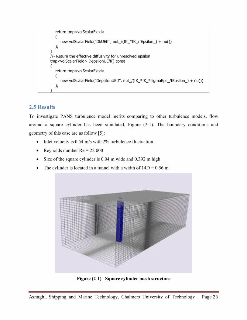
2.5 Results

To investigate PANS turbulence model merits comparing to other turbulence models, flow

around a square cylinder has been simulated, Figure (2-1). The boundary conditions and

geometry of this case are as follow [5]:

• Inlet velocity is 0.54 m/s with 2% turbulence fluctuation

• Reynolds number Re = 22 000

• Size of the square cylinder is 0.04 m wide and 0.392 m high

• The cylinder is located in a tunnel with a width of 14D = 0.56 m

Figure (2-1) –Square cylinder mesh structure


To compare PANS turbulence model with other turbulence models, OEEVM has been selected

from LES turbulence family, and from RANS turbulence family, kEpsilon has been selected.

Drag coefficients and Strouhal number for these three different turbulence models have been

compared with experimental data, Table (2-1). Results show that PANS results are very

promising and are in very good agreement with experimental data. Comparing PANS, and its

RANS parent turbulence model kEpsilon shows that by small code developing, it would be

possible to increase the accuracy of results significantly. However, more efforts especially in the

area of CPU cost should be performed to provide appropriate comparison tools.

Next possible steps to improve this work would be:

• Use two-stage PANS model or dynamic version of PANS

• Compare the performance of PANS in higher Reynolds number

• Try to implement PANS in other RANS turbulence models, e. kOmega

Table (2-1) – Comparing different turbulence models results for flow around the

square cylinder, Re=22e3, inlet velocity 0.54 m/s with 2% turbulence fluctuation

Turbulence model Cd Cd Error (%) Strouhal number St. Error (%)

kEpsilon 1.67 -20.5 0.1348 2.12

OEEVM (LES) 2.05 -2.4 0.1333 1

PANS

(fK=0.2, fEpsilon=1.0) 2.11 0.5 0.134 1.5

Reference Value (Exp.) 2.1 ----- 0.132 -----

2.6 Post processing

Analyzing the obtained numerical simulation and comparing them with experimental data could

be very time consuming task. To reduce the difficulty of this task, several libraries have been

added to the OpenFoam which using them during simulation for data gathering can increase the

simplicity of post processing analyses. In the following, one script to collect data at probe


locations, to calculate drag and lift forces, and to calculate mean fields for pressure, velocity,

turbulence intensities, and etc. has been described.

functions

{

probes

{

type probes;

functionObjectLibs ("libsampling.so");

enabled true;

outputControl timeStep;

outputInterval 1;

probeLocations

(

( 0.05 0.0 0.002 )

( 0.05 0.01 0.002 )

);

fields

(

p

);

}

forces

{

type forceCoeffs;

functionObjectLibs ( "libforces.so" );


outputInterval 1;

patches

(

walls

);

directForceDensity no;

pName p;

UName U;

rhoName rhoInf;

rhoInf 994.5;

CofR ( 0 0 0 );

liftDir ( 0 1 0 );

dragDir ( 1 0 0 );

pitchAxis ( 0 0 1 );

magUInf 0.54;

lRef 0.04;

Aref 0.0157;

Aref1 0.004;

rhoRef 994.5;

}

fieldAverage1

{

type fieldAverage;


functionObjectLibs ("libfieldFunctionObjects.so");

enabled true;

outputControl outputTime;

fields

(

U

{

mean on;

prime2Mean on;

base time;

}

p

{

mean on;

prime2Mean on;

base time;

}

);

}

}

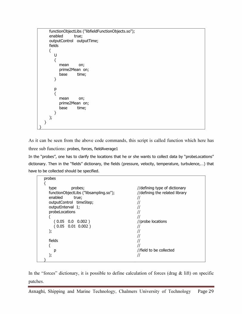
As it can be seen from the above code commands, this script is called function which here has

three sub functions: probes, forces, fieldAverage1

In the “probes”, one has to clarify the locations that he or she wants to collect data by “probeLocations”

dictionary. Then in the “fields” dictionary, the fields (pressure, velocity, temperature, turbulence,…) that

have to be collected should be specified.

probes

{

type probes;

functionObjectLibs ("libsampling.so");

enabled true;


outputInterval 1;

probeLocations

(

( 0.05 0.0 0.002 )

( 0.05 0.01 0.002 )

);

fields

(

p

);

}

//defining type of dictionary

//defining the related library

//

//

//

//

//

//probe locations

//

//

//

//

//

//field to be collected

//

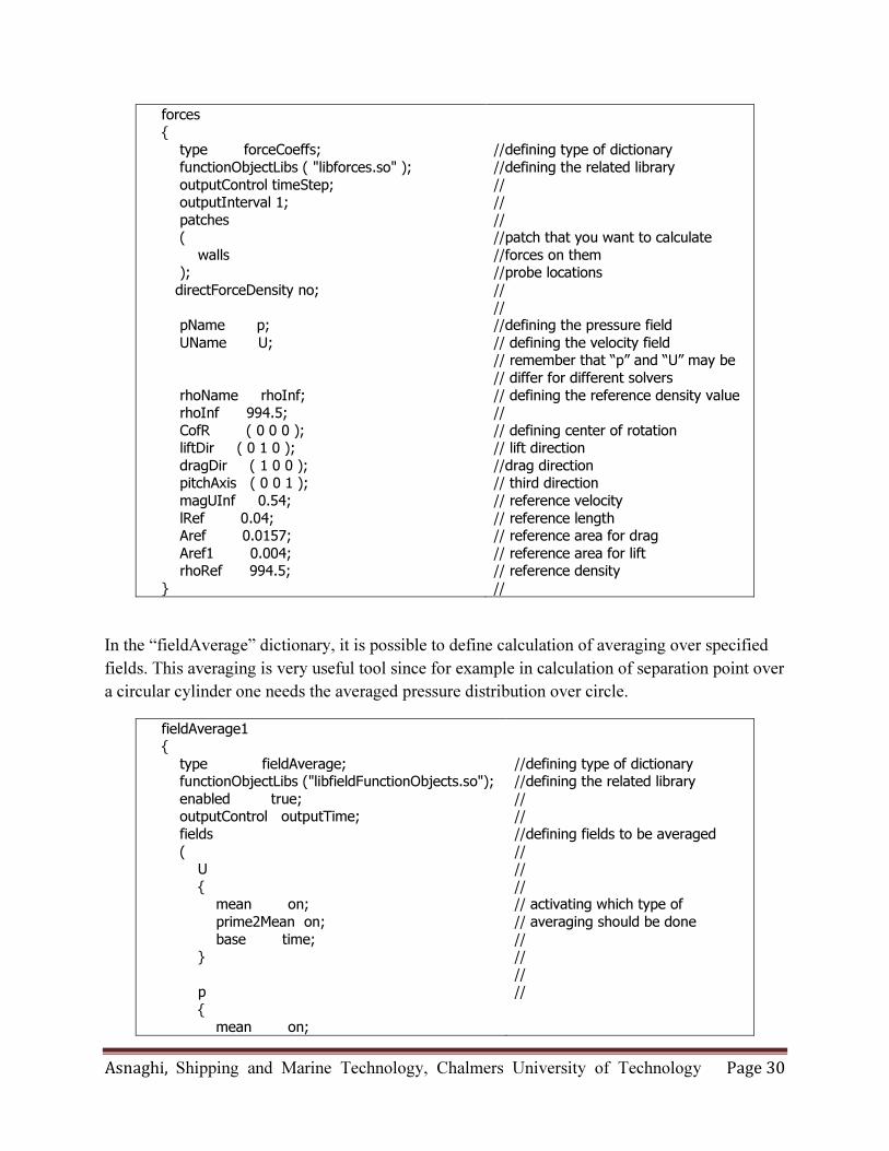
In the “forces” dictionary, it is possible to define calculation of forces (drag & lift) on specific

patches.


forces

{

type forceCoeffs;

functionObjectLibs ( "libforces.so" );


outputInterval 1;

patches

(

walls

);

directForceDensity no;

pName p;

UName U;

rhoName rhoInf;

rhoInf 994.5;

CofR ( 0 0 0 );

liftDir ( 0 1 0 );

dragDir ( 1 0 0 );

pitchAxis ( 0 0 1 );

magUInf 0.54;

lRef 0.04;

Aref 0.0157;

Aref1 0.004;

rhoRef 994.5;

}



//

//

//

//patch that you want to calculate

//forces on them

//probe locations

//

//

//defining the pressure field

// defining the velocity field

// remember that “p” and “U” may be

// differ for different solvers

// defining the reference density value

//

// defining center of rotation

// lift direction

//drag direction

// third direction

// reference velocity

// reference length

// reference area for drag

// reference area for lift

// reference density

//

In the “fieldAverage” dictionary, it is possible to define calculation of averaging over specified

fields. This averaging is very useful tool since for example in calculation of separation point over

a circular cylinder one needs the averaged pressure distribution over circle.

fieldAverage1

{

type fieldAverage;

functionObjectLibs ("libfieldFunctionObjects.so");

enabled true;

outputControl outputTime;

fields

(

U

{

mean on;

prime2Mean on;

base time;

}

p

{

mean on;



//

//

//defining fields to be averaged

//

//

//

// activating which type of

// averaging should be done

//

//

//

//


prime2Mean on;

base time;

}

);

}

3. References

1- R. E. Bensow & C. Fureby (2007) On the justification and extension of mixed models in

LES, Journal of Turbulence, 8, N54, DOI: 10.1080/14685240701742335

2- GIRIMAJI, S. S., “Partially-averaged Navier-Stokes method for turbulence: A Reynolds

averaged Navier-Stokes to direct numerical simulation bridging method”, Journal of Applied

Mechanics, Vol 73, page 413-421, 2006

3- http://www.cfd-online.com/Wiki/Standard_k-epsilon_model, Last Checked:14 Oct 2013

4- GIRIMAJI, S., JEONG, E. & SRINIVASAN, R., “Partially averaged Navier-Stokes

method for turbulence: Fixed point analysis and comparison with unsteady partially averaged

Navier-Stokes”, Journal of Applied Mechanics, Vol 73, page 422-429, 2006

5- Sharath Girimaji and Khaled Abdol-Hamid, “Partially-Averaged Navier Stokes Model for

Turbulence: Implementation and Validation”, 43rd AIAA Aerospace Sciences Meeting and

Exhibit. January 2005, Reno, Nevada

6- Henrik Rusche, PhD 2002, page 117, Equation 3.58, access through:

http://foamcfd.org/resources/theses.html

7- NaiXian Lu report for the course “MSc/PhD course in CFD with OpenSource software“

entitled as “Tutorial: Solve Cavitating flow around a 2D hydrofoil using a user modified

version of interPhaseChangeFoam“, 2008

8- A. Asnaghi, E. Jahanbakhsh, M. S. Seif, “Implementation of phase change thermodynamic

probability for unsteady simulation of cavitating flows”, International Journal for Numerical

Methods in Fluids, Volume 66, Issue 12, pages 1555–1571, 30 August 2011

CFD with OpenSource Software - Chalmershani/kurser/OS_CFD_2013/AbolfazlAsnagi/interP... · Asnaghi,...

Documents

Transcript of CFD with OpenSource Software - Chalmershani/kurser/OS_CFD_2013/AbolfazlAsnagi/interP... · Asnaghi,...