1

CFD simulation of the free surface flow

around a full scale oar blade. Master Thesis report.

Presented by: Jacobo Carrasco Heres.

Master thesis Advisor: Alban Leroyer.

Erasmus Mundus Masters of Science in Computational Mechanics, 2008-2010.

Laboratoire de Mécanique des Fluides, UMR CNRS 6598

2

Acknowledgments:

First of all, I want to thank all the teachers of the Masters program, since they all made

possible the masters course. I want to thank them as well since they all left a personal

mark in me. The classes I liked the most were always due to outstanding teaching. I want

to thank specially teachers that were available for me, whether it was for explaining

something I had doubts about but particularly teachers that were available just for talking.

I want to thank the Master Directors both in Barcelona and Nantes, professors Nicolas

Moes and Pedro Diez for being always willing to hear us, and willing to help us, as well as

professor Nicolas Chevaugeon. I want to thank as well the non-teaching staff for their

support and orientation at different points during the Masters.

I want to thank a lot all the researchers of the Equipe de Modélisation Numérique du

Laboratoire de Mécanique des Fluides de l’Ecole Centrale de Nantes, for all their

willingness to help, and for their great advise during this project.

I want to thank Professor Cartraud for his help to get an internship, and for his trust.

I want to say a big thank you to my thesis advisor Alban Leroyer, who was always available

and was very present during the development of my thesis project. I want to thank him for

his guidance, and for proposing a subject that suited my interests and that kept me

interested for its whole duration. I want to thank him for his help on this report, and for all

the time and work that he devoted to me.

I want to thank as well my friends and classmates of the masters program, for their

support and help, and because they helped me to finish the masters course.

It might be slightly unusual, but I want to thank a lot Violette Bruillard, her boyfriend and

her family, since they helped me a lot and made my life easier and better from the

moment I arrived in France. My life is much better because I met her, and I am deeply

grateful to all of them. The students from the Ecole Centrale as well were really

welcoming, and that is something I appreciated a lot, since because of that I had a great

experience here in France.

Finally, I want to thank my parents since they raised me with the idea of getting a good

education, because they taught me to work hard, and for their support (this includes my

brother) and motivation.

I think that all of this enabled me to complete the masters course, and to make the most

out of it.

3

Index.

1. Abstract. 4

2. Introduction. 5

2.1 Configuration of the boat-row system. 5

2.2 Previous results and state of the art. 6

2.3 Mathematical tools to manipulate the movement input. 7

2.3.1 Cardan angles. 7

2.3.2 Quaternions. 8

3. Methods. 11

3.1 Imposed motion. 11

3.1.1 Simple imposed motion. 13

3.1.2 Enhanced kinematic model of motion. 18

3.2 Shaft Flexibility. 22

4. Simulation, pre and post-processing. 30

4.1 Pre-processing. 30

4.1.1 Kinematic motion formatting. 30

4.1.2 Blade modeling. 31

4.1.3 Meshing the blade and its domain. 33

4.2 Configuration of the simulation. 38

4.2.1 Positioning the domain. 38

4.2.2 Configuration of the flow solver parameters. 39

4.3 Post-processing. 40

5. Results and Discussion. 45

6. Bibliography. 46

7. Appendix 1. 47

8. Appendix 2. 49

4

1.- Abstract.

The project consisted in the computation of the flow around a rowing blade with the Isis

CFD software, involving unsteady 3D flow with violent free surface motion, and including

some realistic conditions. The improvements are the implementation of the shaft

flexibility into the software Isis CFD, the consideration of a more realistic kinematic model

of motion that better describes the rowing movement, the simulation will use an

automatic grid refinement technique, and a real oar blade. Animation and post-processing

tools were also developed to complete the work.

5

2.- Introduction:

The purpose of the project is to perform a study of the flow around an oar blade. It

intends to consider realistic conditions, and to develop some tools for the processing of

the results of the simulation. The motion of the blade that is fed to the simulation is

treated with Matlab, and the flexibility of the blade is coded into the Isis-CFD software

(written in FORTRAN). The post-processing consists of an animation in VRML format and in

script language tools for Linux, which can deal with the outputs of Isis CFD.

To study the flow around the oar-blade, different steps were necessary to characterize the

simulation. The first step of the simulation was the geometric description, continuing with

considerations for the models used, then considering a new kinematic description and

finally the flexibility of the oar consideration.

2.1-Configuration of the boat-row system

The simulation of the flow around the oar-blade uses a single solid body that is the blade.

However, the real system is a boat and an oar. A blade by itself is meaningless in real life,

it depends on the system around it, namely the shaft and the boat. However, for the CFD

simulation only the blade is used, but its movement must include a contribution of the

movement of the boat, and the flexibility of the shaft, so even if they are not present, they

are considered. The blade used for the simulation is a numerisation of a competition

blade, in contrast to previous simulations where a simplified rectangular blade was used.

The results from the CFD calculations are compared to experimental results obtained with

an experimental device attached to a carriage, that reproduced the simplified motion that

is later presented. This experimental system reproduces the behavior of a boat with an

oar. The experimental device, shown in figure 1, is the mechanism that enables the

movement of the blade, and is attached to the carriage.

6

Fig. 1: Experimental device that reproduces blade motion, image taken from [2].

2.2- Previous results and state of the art.

The present project builds up on the results obtained from two articles (Leroyer et al.

2008, 2009), which consider a simplified blade, and a simplified imposed motion, in two

different configurations. The two configurations studied in the previous articles are

referred to as [1] and [2], and they include different initial parameters which shape the

imposed motion among other differences. Both articles show results that match

satisfactorily experimental results. Article [1] aimed at validating the capabilities of the

Isis-CFD Reynolds-Averaged Navier-Stokes Equations solver developed at the Fluid

Mechanics Laboratory of Ecole Centrale de Nantes to compute the flow around the blade

of a row (Leroyer et al. 2008).

Once the code’s results were validated, article [2] meant to evaluate the influence of free

surface, unsteadiness and viscous effects in the modeling of the hydrodynamic forces on

blades during a rowing stroke (Leroyer et al. 2009). Previous models and studies neglected

the effects of such parameters, and so one of the goals of the study was to assess their

7

importance. The results show that the free surface has a big impact on the fluid forces,

namely the lift and the drag. Unsteadiness is proven as well to be important to capture

the whole physics of the phenomenon accurately. Both considerations modify the values

obtained for the forces.

In article [5], Maccrossan studies backsplash, that is, the splashing of water towards the

bow of a boat at the moment of the catch of the oar. It analyses the rowing characteristics

of an elite athlete, so it shows accurate measures of a rowing stroke. It describes the

rowing movement and the configuration in a lot of detail. It is interesting because even if

they use different kinematics, the motion they study is similar to ours.

2.3- Mathematical tools to manipulate the movement input.

To manipulate the input for the Isis CFD flow solver, Cardan angle representation and

quaternions were used.

2.3.1-Cardan Angles

Cardan Angle representation is used to describe the orientation of the oar, decomposing it

into three successive rotations. The angles psi, theta and phi stand for yaw, pitch and roll

respectively. The yaw represents the rotation around the z axis, the pitch around the y

axis, and the roll around the x axis. This sequence of rotations describes accurately the

orientation of an object but it is not commutative (it must be performed in this order).

Fig.2: Reference axis for the blade and its’ Cardan Angles.

Yaw Ψ

Roll Φ

Pitch Θ

Z

Y

X

8

To illustrate the Cardan angles further, the pitch angle tells if the blade enters the water

or if it is outside. The roll describes the rotation of the blade with respect to the shaft’s

axis, while the yaw angle describes the fan movement where the oar describes almost a

semi-circle.

2.3.2-Quaternions

Quaternions can be seen as four element vectors that are very convenient to represent

rotations in space. They have a very good mathematical performance and hence they will

be used to represent the orientation with the Cardan angles. A single quaternion contains

the angle and axis of rotation describing the orientation, and so quaternion operations

enable us to represent the complete rotation with a single resulting quaternion.

Q=

𝑄𝑜𝒆𝑄1𝒊𝑄2𝒋𝑄3𝒌

(1)

The orientation of a body can be described by the product of three successive rotations by

the cardan angles. Three quaternions will be defined, containing each one a cardan angle.

The term 𝑄𝑜𝒆 can be considered the real part, and the terms 𝑄1𝒊, 𝑄2𝒋, 𝑄3𝒌, can be

considered the pure part, and can be compared to a vector. In the case of quaternions

representing cardan angles, the real part will contain the angle, and the vector will contain

the rotating axis.

Q= cos

𝛼

2

𝒏 sin𝛼

2

(2)

The rotation of angle 𝛼 around the axis n represents the three cardan angle rotations.

Quaternion operations will thus be necessary to manipulate the three successive simple

rotations that give the orientation. The quaternion basic operations are the following,

given:

Q=

𝑄𝑜𝒆𝑄1𝒊𝑄2𝒋𝑄3𝒌

(3)

9

P=

𝑃𝑜𝒆𝑃1𝒊𝑃2𝒋𝑃3𝒌

(4)

The addition rule for quaternions is component-wise addition, just like with normal

vectors.

For multiplication however, we have to consider the multiplicative properties of elements

i,j,k,

𝑖2 = 𝑗2 = 𝑘2 = ijk = -1, (5)

ij=-ji=-k, (6)

ik=-ki=j, (7)

jk=-kj=-I (8)

Which yields:

QP= 𝑄𝑜 𝒆 + 𝑄1 𝒊 + 𝑄2 𝒋 + 𝑄3 𝒌 𝑃𝑜 𝒆 + 𝑃1 𝒊 + 𝑃2 𝒋 + 𝑃3 𝒌 =

= 𝑄𝑜𝑃𝑜 − 𝑄1𝑃1 − 𝑄2𝑃2 − 𝑄3𝑃3 𝒆 + 𝑄0𝑃1 + 𝑄1𝑃𝑜 + 𝑄2𝑃3 − 𝑄3𝑃2 𝒊 +

+ 𝑄0𝑃2 + 𝑄2𝑃0 + 𝑄3𝑃1 − 𝑄1𝑃3 𝒋 + 𝑄0𝑃3 + 𝑄3𝑃0 + 𝑄1𝑃2 − 𝑄2𝑃1 𝒌 (9)

So, if a rotation is decomposed into three successive simple rotations by the quaternions

of the cardan angles, the total rotation is given by the multiplication of the yaw, pitch and

roll quaternions:

𝑄𝑡 = 𝑄Ψ 𝑄𝛩 𝑄𝛷 (10)

Once the total quaternion representing the rotation is obtained, it has to be applied to the

position vector. To rotate the position vector of the blade, the quaternion of the final

rotation has to be put in a Passage Matrix, which will perform the transformation. The

passage matrix containing a quaternion is defined as follows:

MP =

2 𝑞02 + 𝑞1

2 − 1 2 𝑞1𝑞2 − 𝑞0𝑞3 2 𝑞1𝑞3 + 𝑞0𝑞2

2 𝑞1𝑞2 + 𝑞0𝑞3 2 𝑞02 + 𝑞2

2 − 1 2 𝑞2𝑞3 − 𝑞0𝑞1

2 𝑞1𝑞3 − 𝑞0𝑞2 2 𝑞2𝑞3 + 𝑞0𝑞1 2 𝑞02 + 𝑞3

2 − 1

(11)

10

This matrix will then be multiplied by the position vector to obtain the rotated vector. This

is used as well for the rotation due to flexibility, which uses passage matrices to orient the

shaft vector and the force.

11

3.-Methods:

The purpose of the project is to perform a simulation with more realistic considerations.

To prepare the simulation, the motion of the boat had to be imposed, for which an

enhanced kinematic model of motion was used; the flexibility of the shaft, which was

previously considered to be completely rigid, had to be considered. Automatic grid

refinement was used, as it reduces the computational cost of simulations and because it

improves the quality of the results.

First of all, a simulation was configured reproducing the movement laws used in [1], to

have a comparison point with the previous results, and from there new features were

added to the simulation, building to a new completer one.

3.1-Imposed motion

The blade motion is constructed considering the movement of the boat and the

movement of the row. The boat is moving forward, in the positive X direction, while the

oar had a more complex movement, with rotations on the three axes. The accuracy and

smoothness of the motion input is very important for the stability and accuracy of the

results, so it is advisable to use quite small time steps to discretize the movement. Failing

to discretize adequately the results can result in the calculation diverging quickly.

Simulations were launched testing two different cases, an imposed motion given by

formulas, which was already tested in other publications ([1] and [2]), and an enhanced

kinematic model of motion that included the catch and the finish of the row, as well as the

natural movement of the boat in the water, which is a more accurate representation. The

first configuration is helpful as a test case study, since results exist for these conditions.

The new proposed model of motion however has no reference for comparison.

The following figure illustrates the boat and the row, and shows the global reference for

the model of motion.

12

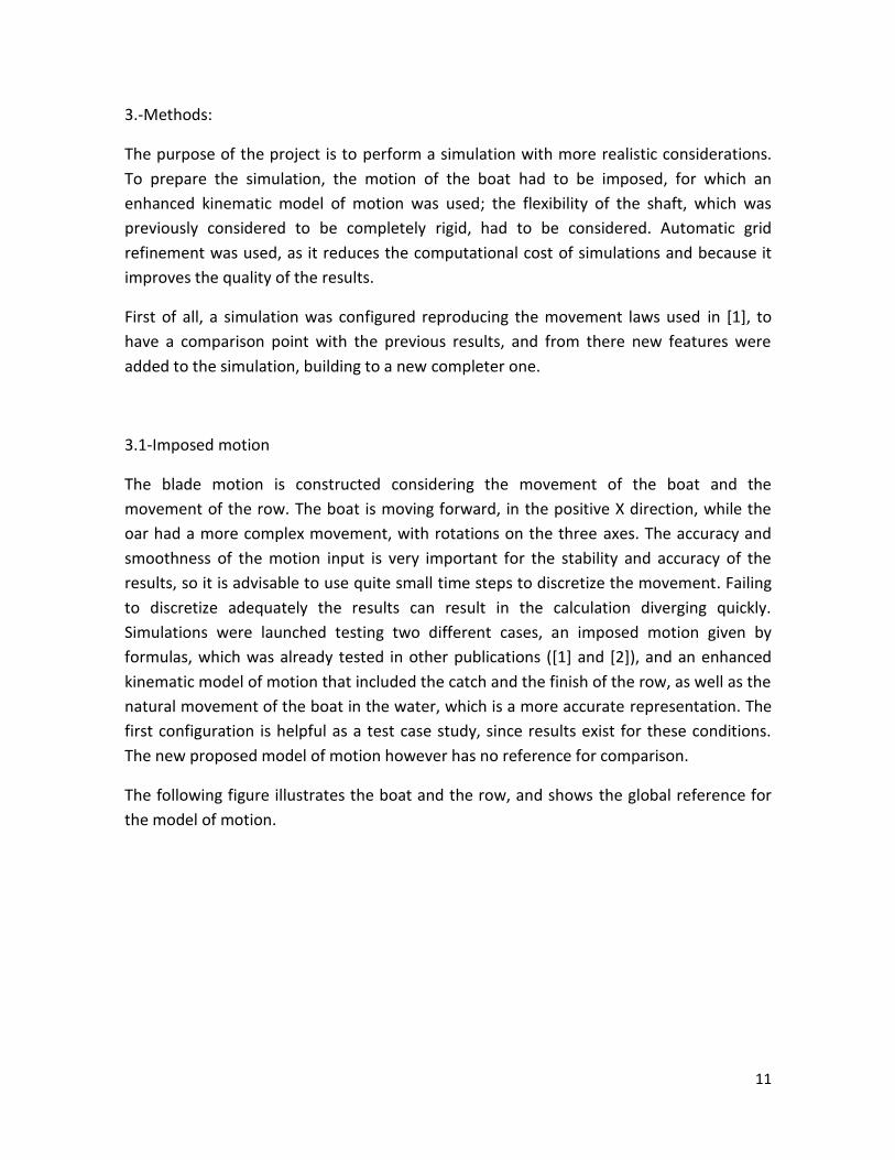
Fig. 3: Boat and oar system.

This figure represents the whole system that is studied, even if in the simulation the only

actual body is the blade. However, this drawing helps visualize the system and understand

the rowing motion. The boats’ front corresponds to the side with the black circle, and that

is the direction of the boats’ movement. The Origin for the model of motion ( the global

reference ) is on the axis of the geometric center of the boat (for the x and y coordinates),

and it is located on the surface of the water ( for the z coordinate ), which is the free

surface. The points 1 and 2 on the oar signal the point where the shaft joins the blade, and

the oarlock, according to the configuration used in [1]. Point 1 is the point where the

movement of the blade is defined. The movement files that are fed to Isis CFD all refer to

this point. Point 2, the oarlock, is only used as a reference to locate the blade and to

establish its rotation, but it is not really used for anything else. However, for the new

simulation considering a real blade and flexibility, there is a small difference. Point 1 is still

the same point, where we will define movement, apply the force, and where we will

impose flexibility (flexibility is considered through a motion correction), but point 2 is

rather the point where the sensor for the reaction is.

However, the position of the oar in the figure is not its actual initial position and

orientation. Point 1’s starting site is rather physically located at,

13

[0.9289, 2.0105, 0.2478],

while the oarlock is correctly located at,

[0, 0.838, 0.375].

In the second case, where Point 2 rather signals the sensor, it is located at 0.441m from

the oarlocks position.

This initial position is shown because it illustrates well the system, and because that

orientation was used for meshing, since it simplified the process. Having the oar blade

aligned initially with the x axis was useful, since that made the mesh more regular. Having

the body parallel to the domain made the cells around it more regular and allowed having

a coarser mesh, since the body “respects” the direction of the mesh generation.

3.1.1 Simple imposed motion.

A simple imposed motion was programmed, reproducing the input motion described in

[1]. A program was written in MATLAB that creates the input files for Isis CFD, both for the

imposed motion explained in this section, or the new kinematic model that includes the

whole movement, from before the catch of the oar, the movement under water, and

lastly the finish of the oar. This new movement description will be explained later in the

report.

The boat starts at rest completely still, and then it starts moving in the positive X direction,

following a quarter-sinus law that leads it to its final velocity, where it stays constant. The

final velocity varies depending on the configuration used ([1] or [2]). The transition from

rest to the final constant velocity is given by:

𝑣𝑒𝑙(𝑖) = 𝑉𝑓 ∙ sin(

𝜋

2 ∙

𝑡𝑖

𝑡𝑡ℎ𝑟𝑒𝑠 ℎ𝑜𝑙𝑑) 𝑡𝑖 < 𝑡𝑡ℎ𝑟𝑒𝑠ℎ𝑜𝑙𝑑

𝑉𝑓 𝑡𝑖 ≥ 𝑡𝑡ℎ𝑟𝑒𝑠ℎ𝑜𝑙𝑑

(12)

Then the velocity of the boat is integrated to obtain its displacement, since the simulation

rather uses the displacement. The displacement is given by:

𝑑𝑖𝑠𝑝 (𝑖) = 𝑉𝑓 ∙

2 ∙ 𝑡𝑡ℎ𝑟𝑒𝑠 ℎ𝑜𝑙𝑑

𝜋 ( 1 − cos

𝜋

2 ∙

𝑡𝑖

𝑡𝑡ℎ𝑟𝑒𝑠 ℎ𝑜𝑙𝑑 ) 𝑡𝑖 < 𝑡𝑡ℎ𝑟𝑒𝑠ℎ𝑜𝑙𝑑

𝑑𝑖𝑠𝑝𝑖−1 + 𝑉𝑓 ∙ 𝑡𝑖 − 𝑡𝑖−1 𝑡𝑖 ≥ 𝑡𝑡ℎ𝑟𝑒𝑠ℎ𝑜𝑙𝑑

(13)

14

The input blade motion for the simulation considers the blade movement and its

orientation. The motions’ x component is the result of the boat movement and the

addition of the rotation of the blade. The y component of motion is completely given by

the row motion, while the z component of motion stays constant, since in this simplified

case, we consider that the blade is already submerged in the water and that it stays put at

that height. We then have to give as well the orientation of the oar-blade, which is mainly

the result of the rowing motion. The orientation of the oar is described by the Cardan

angles psi, theta and phi (yaw, pitch and roll respectively). These angles are first defined,

and then manipulated using quaternion operations to obtain the components of

displacement and orientation. However, for the simplified motion, the only angular

movement is the yaw, and we consider zero the pitch and roll.

The yaw movement is the main part of the movement since it is the actual rowing. It is

given by:

Ψ = 2 ∙ tan−1 𝑒𝐾 𝑡𝑖−𝑡0−𝑡Ψ 𝑡𝑖 ≥ 𝑡Ψ

𝑎 + 𝑏 𝑡𝑖 − 𝑡Ψ + 𝑐 𝑡𝑖 − 𝑡Ψ 2 𝑡𝑖 < 𝑡Ψ (14)

The motion’s initial transitory period is given by a Parabolic Junction law, which gives the

constants a, b, c, while K, t0 and 𝑡Ψ are given by the experimental configuration. The

parabolic junction law is used to reduce the velocity discontinuity at 𝑡Ψ . Smoothening

discontinuities and avoiding big leaps in the behavior is important to avoid triggering

divergence, which is a difficult issue for many simulations.

𝑎 = 2 ∙ tan−1 𝑒𝐾 −𝑡0 (15)

𝑏 = 𝐾 ∙ sin 2 ∙ tan−1 𝑒𝐾 −𝑡0 (16)

𝑐 = 𝑏2

4 𝑎 (17)

The pitch describes the catch and the finish of the rowing movement, but it was

considered zero in [1] and [2]. The catch is the moment when the oar blade touches and

enters the water, while the finish is the opposite, the moment when the oar has

completed its displacement on the water and comes out. When studying the enhanced

movement, the catch and the finish are considered, including even the contribution of the

natural tilting of the boat due to the movement of water.

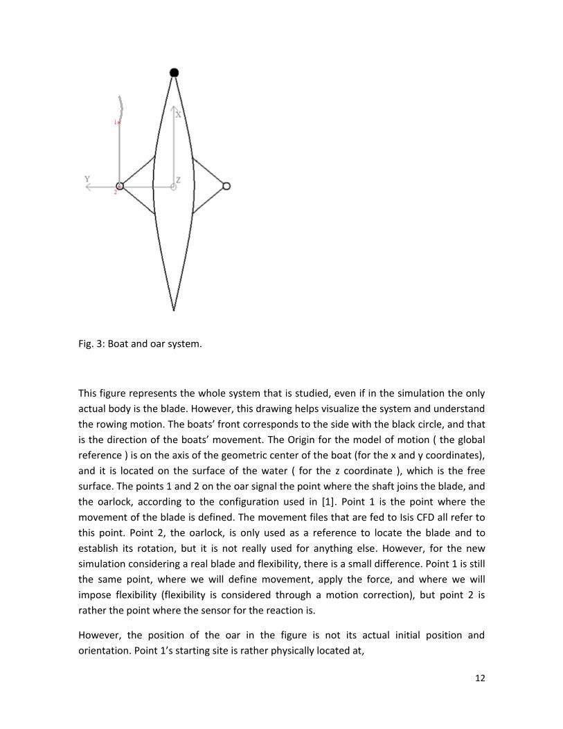
The simplified motion is illustrated in figure 4, that shows the oar blade displacement and

rotation at different time steps through its entire span.

15

Fig. 4: Prescribed motion of the blade, taken from [2]

The following are the quaternions of the yaw, pitch, and roll

Qyaw=

cos

Ψ

2

00

sinΨ

2

(18)

Qpitch=

cos

𝜃

2

0

sin𝜃

2

0

(19)

Qroll=

cos

Φ

2

sinΦ

2

00

(20)

16

which are then orderly multiplied to obtain the total quaternion, which represents the

whole rotation.

Finally the movement due to the boat and the movement of the blade are added to obtain

the final displacement which is fed to the simulation.

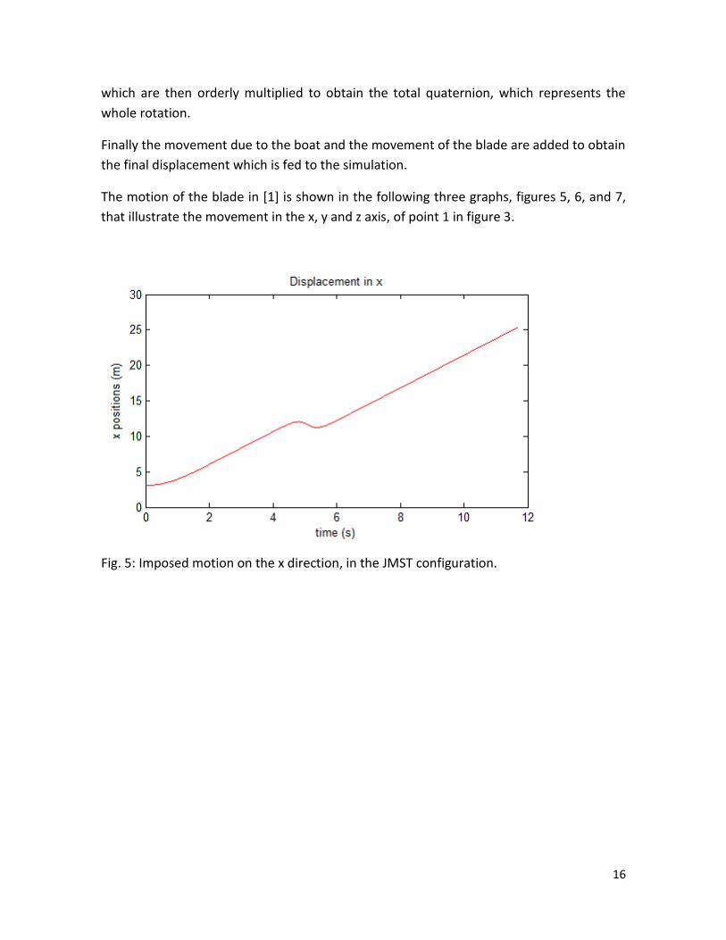
The motion of the blade in [1] is shown in the following three graphs, figures 5, 6, and 7,

that illustrate the movement in the x, y and z axis, of point 1 in figure 3.

Fig. 5: Imposed motion on the x direction, in the JMST configuration.

17

Fig. 6: Imposed motion on the y direction, in the JMST configuration.

Fig. 7: Imposed rotation motion, in the JMST configuration.

As we can see, the blade moves quite smoothly and regularly, but in the two-second

period between 4 and 6s, the blade turns around, and we see the effect of the rotation in

18

the x and y components of motion as well. We can see it on the x component as the

movement decreases for a short leap of time, until the blade stops rotating and the

positive direction displacement continues. The effect on the y component is even clearer,

since y keeps constant, except for the time period of the rotation, where there is a peak in

the movement.

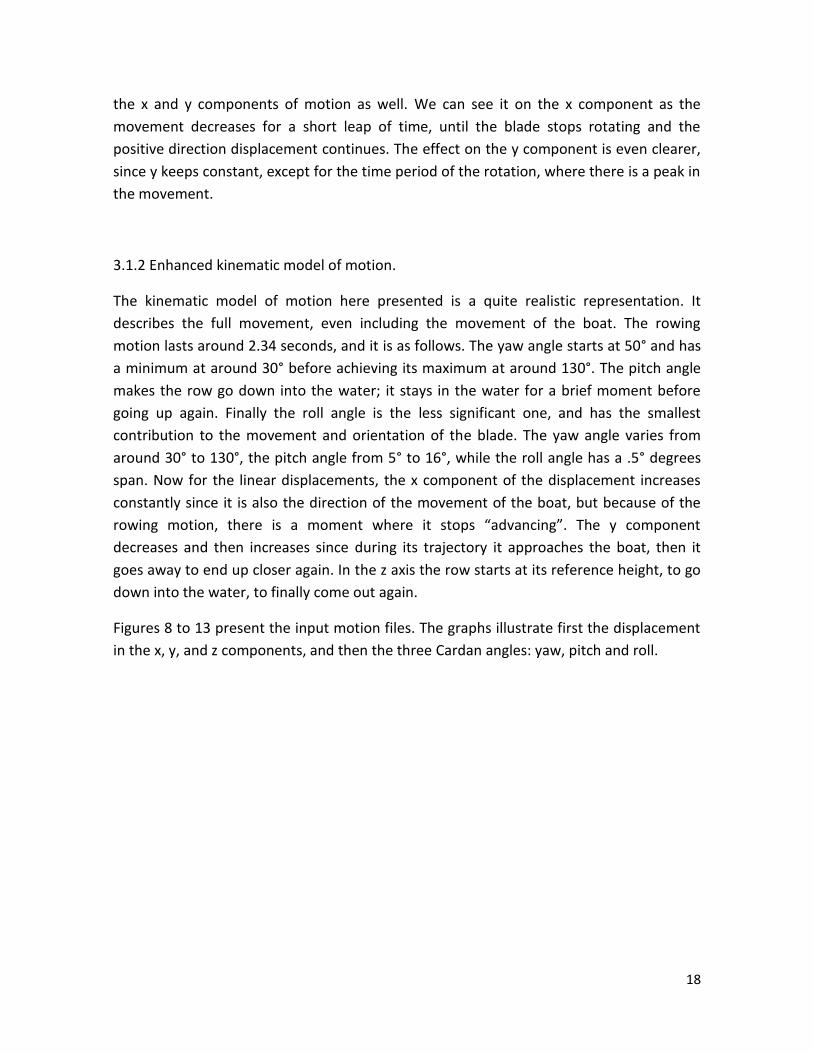
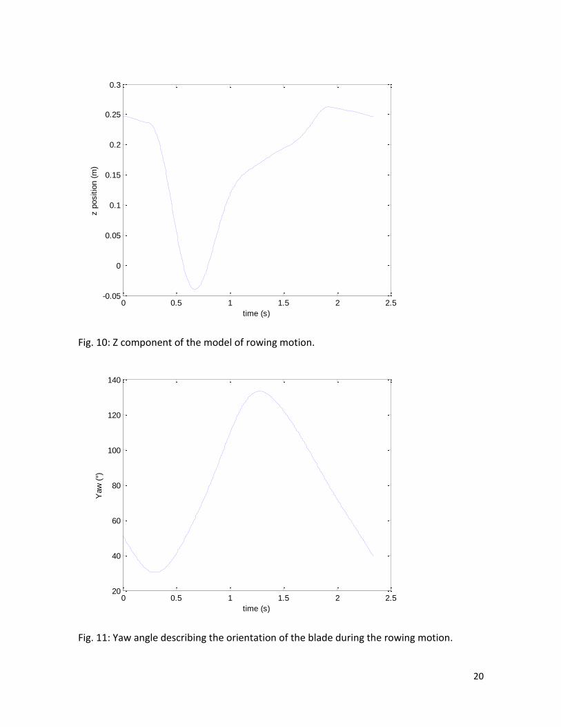
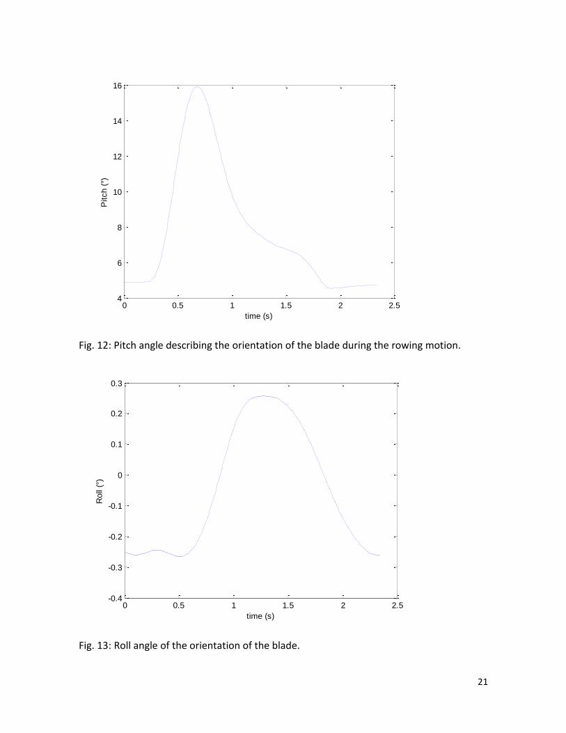
3.1.2 Enhanced kinematic model of motion.

The kinematic model of motion here presented is a quite realistic representation. It

describes the full movement, even including the movement of the boat. The rowing

motion lasts around 2.34 seconds, and it is as follows. The yaw angle starts at 50° and has

a minimum at around 30° before achieving its maximum at around 130°. The pitch angle

makes the row go down into the water; it stays in the water for a brief moment before

going up again. Finally the roll angle is the less significant one, and has the smallest

contribution to the movement and orientation of the blade. The yaw angle varies from

around 30° to 130°, the pitch angle from 5° to 16°, while the roll angle has a .5° degrees

span. Now for the linear displacements, the x component of the displacement increases

constantly since it is also the direction of the movement of the boat, but because of the

rowing motion, there is a moment where it stops “advancing”. The y component

decreases and then increases since during its trajectory it approaches the boat, then it

goes away to end up closer again. In the z axis the row starts at its reference height, to go

down into the water, to finally come out again.

Figures 8 to 13 present the input motion files. The graphs illustrate first the displacement

in the x, y, and z components, and then the three Cardan angles: yaw, pitch and roll.

19

Fig. 8: X component of the model of rowing motion.

Fig. 9: Y component of the rowing model of motion.

0 0.5 1 1.5 2 2.50

2

4

6

8

10

12

time (s)

x p

ositio

n (

m)

0 0.5 1 1.5 2 2.51.6

1.7

1.8

1.9

2

2.1

2.2

2.3

2.4

2.5

time (s)

y p

ositio

n (

m)

20

Fig. 10: Z component of the model of rowing motion.

Fig. 11: Yaw angle describing the orientation of the blade during the rowing motion.

0 0.5 1 1.5 2 2.5-0.05

0

0.05

0.1

0.15

0.2

0.25

0.3

time (s)

z p

ositio

n (

m)

0 0.5 1 1.5 2 2.520

40

60

80

100

120

140

time (s)

Yaw

(°)

21

Fig. 12: Pitch angle describing the orientation of the blade during the rowing motion.

Fig. 13: Roll angle of the orientation of the blade.

0 0.5 1 1.5 2 2.54

6

8

10

12

14

16

time (s)

Pitch (

°)

0 0.5 1 1.5 2 2.5-0.4

-0.3

-0.2

-0.1

0

0.1

0.2

0.3

time (s)

Roll

(°)

22

When comparing the new model of motion we can see that the only component where

there is some similarity is x, where the shape of the curve is similar both for the simplified

motion and for the new motion. In both cases the curve increases until the moment when

the oar rotates, where the displacement is almost compensated by the rotating

movement and hence the blade stops advancing.

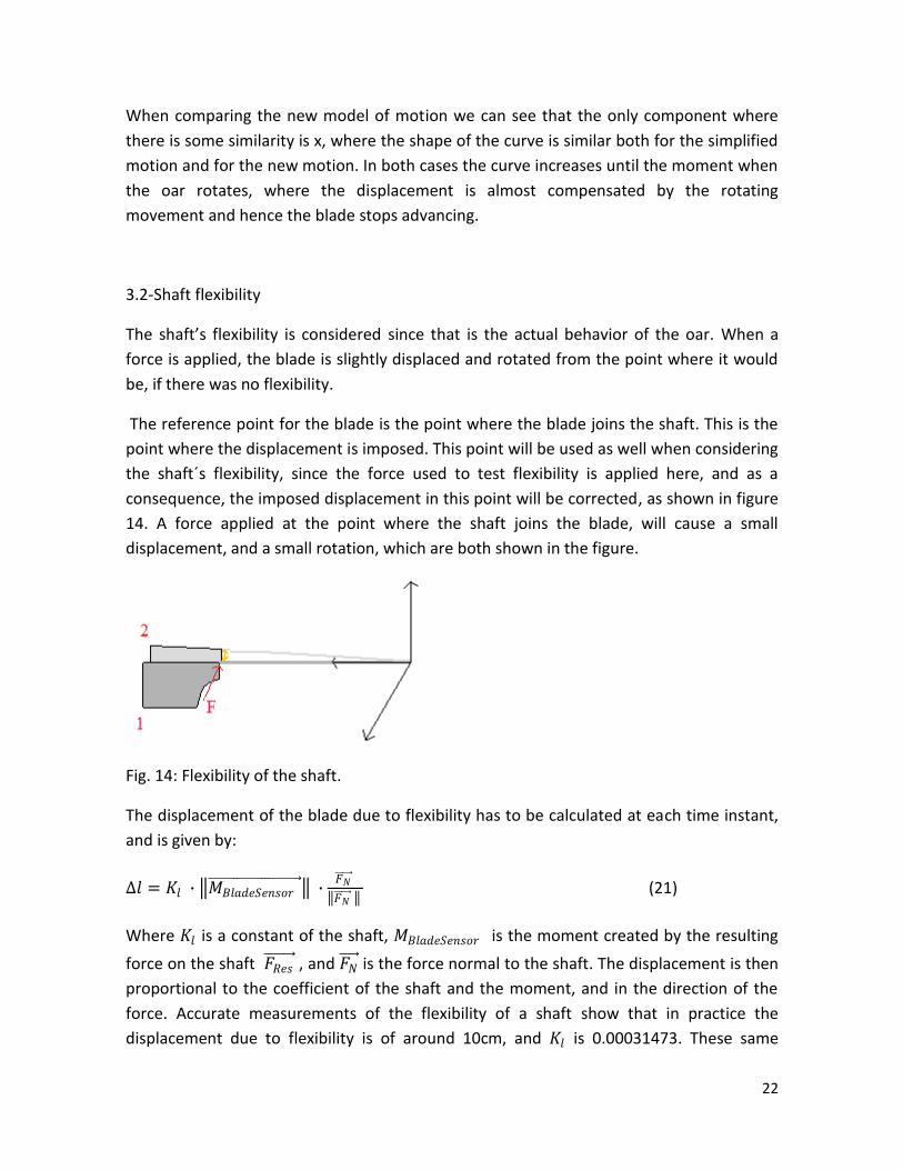
3.2-Shaft flexibility

The shaft’s flexibility is considered since that is the actual behavior of the oar. When a

force is applied, the blade is slightly displaced and rotated from the point where it would

be, if there was no flexibility.

The reference point for the blade is the point where the blade joins the shaft. This is the

point where the displacement is imposed. This point will be used as well when considering

the shaft´s flexibility, since the force used to test flexibility is applied here, and as a

consequence, the imposed displacement in this point will be corrected, as shown in figure

14. A force applied at the point where the shaft joins the blade, will cause a small

displacement, and a small rotation, which are both shown in the figure.

Fig. 14: Flexibility of the shaft.

The displacement of the blade due to flexibility has to be calculated at each time instant,

and is given by:

∆𝑙 = 𝐾𝑙 ∙ 𝑀𝐵𝑙𝑎𝑑𝑒𝑆𝑒𝑛𝑠𝑜𝑟 ∙

𝐹𝑁

𝐹𝑁 (21)

Where 𝐾𝑙 is a constant of the shaft, 𝑀𝐵𝑙𝑎𝑑𝑒𝑆𝑒𝑛𝑠𝑜𝑟 is the moment created by the resulting

force on the shaft 𝐹𝑅𝑒𝑠 , and 𝐹𝑁

is the force normal to the shaft. The displacement is then

proportional to the coefficient of the shaft and the moment, and in the direction of the

force. Accurate measurements of the flexibility of a shaft show that in practice the

displacement due to flexibility is of around 10cm, and 𝐾𝑙 is 0.00031473. These same

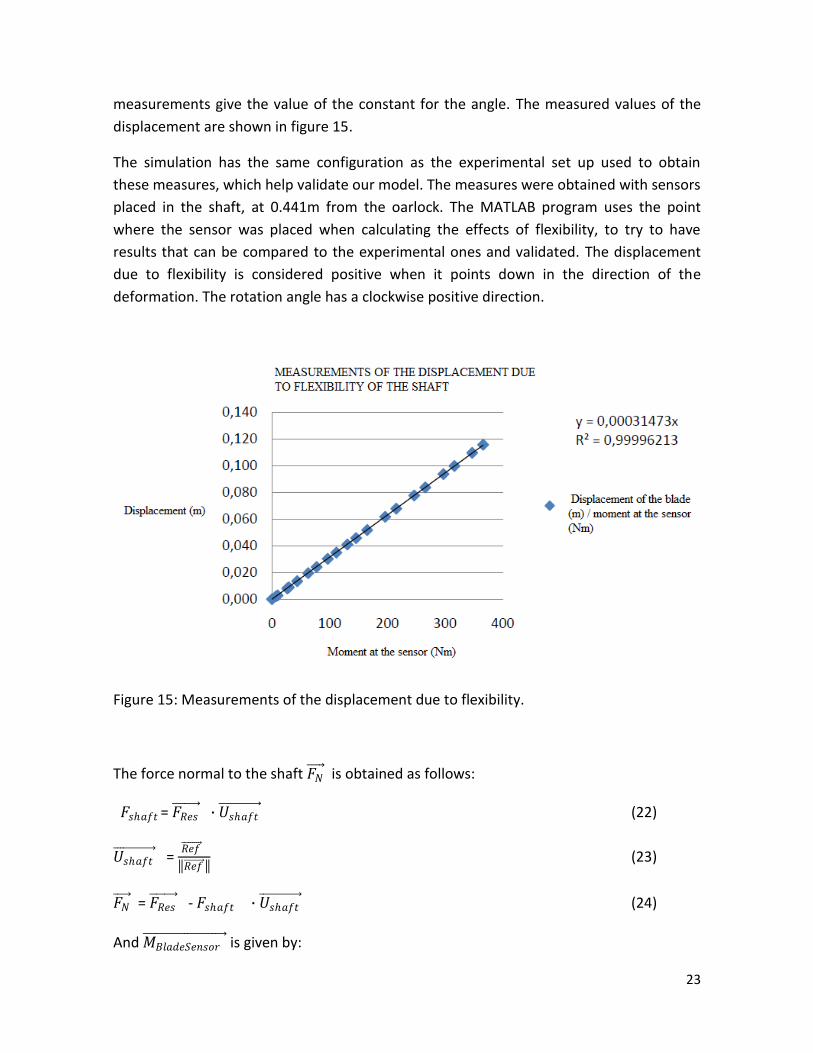
23

measurements give the value of the constant for the angle. The measured values of the

displacement are shown in figure 15.

The simulation has the same configuration as the experimental set up used to obtain

these measures, which help validate our model. The measures were obtained with sensors

placed in the shaft, at 0.441m from the oarlock. The MATLAB program uses the point

where the sensor was placed when calculating the effects of flexibility, to try to have

results that can be compared to the experimental ones and validated. The displacement

due to flexibility is considered positive when it points down in the direction of the

deformation. The rotation angle has a clockwise positive direction.

Figure 15: Measurements of the displacement due to flexibility.

The force normal to the shaft 𝐹𝑁 is obtained as follows:

𝐹𝑠ℎ𝑎𝑓𝑡 = 𝐹𝑅𝑒𝑠 ∙ 𝑈𝑠ℎ𝑎𝑓𝑡

(22)

𝑈𝑠ℎ𝑎𝑓𝑡 =

𝑅𝑒𝑓

𝑅𝑒𝑓 (23)

𝐹𝑁 = 𝐹𝑅𝑒𝑠

- 𝐹𝑠ℎ𝑎𝑓𝑡 ∙ 𝑈𝑠ℎ𝑎𝑓𝑡 (24)

And 𝑀𝐵𝑙𝑎𝑑𝑒𝑆𝑒𝑛𝑠𝑜𝑟 is given by:

24

𝑀𝐵𝑙𝑎𝑑𝑒𝑆𝑒𝑛𝑠𝑜𝑟 = 𝑅𝑒𝑓 × 𝐹𝑅𝑒𝑠

(25)

Where 𝑅𝑒𝑓 is the vector from the sensor to the reference point where the shaft joins the

blade.

Now for the rotation of the blade due to the flexibility of the shaft, the angle that it makes

with respect to the position of the shaft without flexibility is:

∆𝛺 = 𝐾𝛺 ∙ 𝑀𝐵𝑙𝑎𝑑𝑒𝑆𝑒𝑛𝑠𝑜𝑟 (26)

Where again 𝐾𝛺 is a constant of the shaft equal to 0.00038521, obtained from

experimental measurements of flexibility. The angular displacement due to flexibility is

also proportional to the moment. The value of the constant was obtained from

experimental measures, which are shown in figure 16.

Fig. 16: Measurements of the angular displacement due to flexibility.

The axis of rotation for this angle is the unitary vector given by:

𝑒 = 𝑀𝐵𝑙𝑎𝑑𝑒𝑆𝑒𝑛𝑠𝑜𝑟

𝑀𝐵𝑙𝑎𝑑𝑒𝑆𝑒𝑛𝑠𝑜𝑟 (27)

We finally obtain the orientation of the blade with:

𝑄𝑡𝑖 = 𝑄𝑓𝑖

∙ 𝑄𝑖 (28)

25

Where 𝑄𝑡𝑖 is the final quaternion containing the orientation of the blade; 𝑄𝑓𝑖

is the

quaternion containing the rotation due to the flexibility of the shaft, and 𝑄𝑖 is the

quaternion containing the rotation due to the imposed motion of the blade.

𝑄𝑓𝑖 =

cos∆𝛺

2

𝑒 sin∆𝛺

2

(29)

The flexibility function was programmed in FORTRAN to include it in Isis CFD. To validate

the flexibility of the blade, a simple case was tested, in a configuration where the resulting

value is simple enough as to calculate it analytically, and that shows a response that we

know beforehand. The analytical value was calculated as well in Matlab to compare to the

results obtained with Isis CFD.

The analytical configuration that was studied was the case where there is only an imposed

yaw movement, with the force acting on the point where the shaft joins the blade, point 1

of figure 3. The force was imposed in the y, z and x directions to compare the results in

these cases. The results obtained with Matlab and Isis CFD are identical, and they are

shown in figures 19, 20 and 21. This test case used exaggerated values for the constants

of the shaft (in both cases equal to 1), since that illustrates more obviously the result of

flexibility.

Figure 18 shows the imposed movement for the simulation, and the resulting movement

due to the effect of flexibility, with a force of 50N acting on the y axis applied again on

point 1 of figure 3, on the negative direction. These graphs are obtained with matlab, and

illustrate the input movement created for Isis CFD, and the resulting movement that

should be obtained due to the consideration of flexibility. As this force is perpendicular to

the shaft, it causes some moment, and consequently some bending. The bending causes

some linear displacement and a modification of the orientation of the blade. The bending

consequence is a modification of the positions in the x and y axis (upper right and left

graphs respectively), but not in the z one (lower left), as it is shown in the figure. This

figure shows as well the difference in the yaw angle (the modification of the orientation of

the blade), which is shown in the lower right corner. In the case of the yaw angle, the

result of flexibility is introducing some offset into the original trajectory. The main effect

of the flexibility can be seen on the period when the blade is turning, seconds 4 to 6, in

which the movement is significantly modified. Before and after this period, the flexibility

only introduces a small offset into the movement.

26

Fig. 17: Effect of flexibility due to a force applied on the negative y direction.

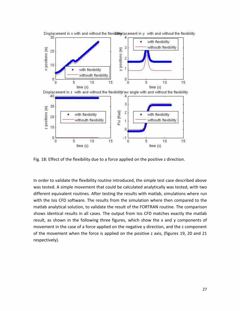
Figure 18 shows the effect of flexibility when the applied force of 50N is applied on the

positive z direction. In this case a peak is present as well on the moment that the blade is

turning. However, as the force is applied on the z axis, there is a very limited effect on x,

while the main impact of the force is seen on the y and z imposed movements. One

difference between the results of the displacement to the previous case is that the force

applied on the z axis introduces an offset in the z component of movement, but without

any peaks. This behavior is quite logical, both in the case of the force applied in the

negative y direction, as well as in this case. In both cases the effect on the yaw angle is

similar.

Finally, imposing a force in the x direction causes no modification or bending whatsoever.

As the force is applied on the axis of the shaft, there is no moment, and the flexibility is

proportional to the moment. The case was considered and tested, but its results are not

shown since they show nothing worth highlighting. The input motion is not displaced, and

the yaw angle remains the same.

27

Fig. 18: Effect of the flexibility due to a force applied on the positive z direction.

In order to validate the flexibility routine introduced, the simple test case described above

was tested. A simple movement that could be calculated analytically was tested, with two

different equivalent routines. After testing the results with matlab, simulations where run

with the Isis CFD software. The results from the simulation where then compared to the

matlab analytical solution, to validate the result of the FORTRAN routine. The comparison

shows identical results in all cases. The output from Isis CFD matches exactly the matlab

result, as shown in the following three figures, which show the x and y components of

movement in the case of a force applied on the negative y direction, and the z component

of the movement when the force is applied on the positive z axis, (figures 19, 20 and 21

respectively).

28

Fig. 19: Comparison of the X component with an applied force on the –y direction.

Fig. 20: Comparison of the y component with an applied force on the –y direction.

29

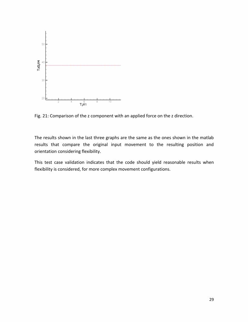
Fig. 21: Comparison of the z component with an applied force on the z direction.

The results shown in the last three graphs are the same as the ones shown in the matlab

results that compare the original input movement to the resulting position and

orientation considering flexibility.

This test case validation indicates that the code should yield reasonable results when

flexibility is considered, for more complex movement configurations.

30

4. Simulation, pre and post-processing.

The complete simulation of the rowing movement required different stages, all of them

leading to a better understanding of the problem, and to a better representation of the

phenomenon. The complete simulation entailed first of all preparing the input files for the

simulation. The second step was the creation and meshing of the body (the blade) and the

domain. Afterwards, the simulation needed configuring, which meant establishing the

physics of the problem, and the hypothesis that enable us to resolve the problem. The

final step of the simulation consists of performing the post-treatment of results.

All the necessary steps to perform the simulation follow a different logic, and they are

performed with different tools. The pre-processing was mainly done using with MATLAB.

To have a realistic blade, a real blade was scanned and the resulting mesh treated to form

a solid. It was then necessary to make sense of a point cluster to define a solid that could

be meshed with a computer aided design software (CAD). The solid and the domain were

put together to create the input mesh for the simulation with a meshing software. The

simulation in Isis CFD was then configured. Finally the results of the simulation are post-

treated. The post-treatment entails treating the output information from Isis CFD to put it

into an intelligible format, which can be compared and which enables us to understand

the result. These is all achieved with graphing tools, both to present the numerical data in

a format which allows easy comparison, and to give results that illustrate the problem

studied.

4.1 Pre-processing.

The pre-processing has three main components, the kinematic motion file treating, the

blade cad model treatment, and the meshing.

4.1.1 Kinematic motion formatting.

The kinematic motion that is fed to the simulation was developed by another team of the

department of fluid mechanics. We received files that give the position and the

orientation of the reference point ( the junction between the shaft and the blade ), and

we only had to format them so that they could be fed to Isis CFD.

The first important consideration for these files is that they give the position and

orientation of the reference point, but what the simulation uses is the displacement so we

31

had to change them. This entailed a simple subtraction of the initial position, which gave

us the real displacement at each time instant.

The motion files use a different reference from the one used for the flexibility law, and

that make the values of the motion and position “inaccessible” or practically

“untouchable”. The reason for this is first of all that the reference is in the center of the

boat and at the free surface level, and not in the oar lock as in the case of the flexibility

law. Then, the oar lock is a complex joint where there is not only rotation but also a slight

displacement ( to model appropriately an oar lock ), and so the position of the reference

point is not as obvious as it would seem.

Finally there is a geometrical consideration that impacts the input kinematic motion files.

The reference point where the shaft joins the blade is physically not on the blade. This

reference point is rather the center of the axis of the shaft, at the height where it reaches

the blade. The shaft and the blade are not aligned and so this point is outside the body of

the blade.

4.1.2 Blade modeling.

A realistic blade was one of the important considerations to be added to improve the

simulation. In previous simulations a rectangular and very simple blade was used. To

upgrade the current simulation, a realistic blade was included. A real blade was scanned

with a sophisticated scanner system that is used industrially to have precise models of

objects. The blade was scanned with the help of Florent Laroche and Fabrice Brau, of the

Ecole Centrale de Nantes. This gave a mesh or point cluster that had to be further treated

to obtain a solid CAD blade model that could be used. This was imported to a meshing

software where its domain was created so they could be meshed and fed to Isis CFD.

The scanner creates automatically a 3D mesh of points of the image. For the scanner to

have some reference, small circular stickers are placed randomly to give it a pattern, so

that it can recognize its position and orientation. Having an appropriate reference for the

scanner is a crucial point for a successful scan, especially around the edges. To capture the

edges adequately, and to enable the scanner to identify the two faces of the blade, as well

as the shaft, round globes were attached to the blades’ corners to smoothen the

transition from one side to the other, and they were removed from the mesh once the

scanning was completed. This gave an accurate model of the blade that was treated

further. The shaft was included on the scanned model, mainly because it was necessary as

reference for the motion and orientation, even if the solid model used doesn’t actually

have the shaft. However, the reference point where the shaft joins the blade is not

32

located on the blade, but rather on the shaft, so that when we removed the shaft, we had

to make sure that we could still find this important reference point.

The Geomagic Studio software was used to clean and make sense out of the mesh of

points obtained from the scanner. This mesh was then transformed into a solid with the

software Rhinoceros. The CAD file output from Geomagic contained enough points to

create the faces of the oar blade, and to orient its shaft, even if the shaft was not

completely scanned. Some traces on the model allowed us to build a circular solid shaft

that was used only to orient the blade. The scanner takes as first reference or world

reference the normal of its first scan, so the model it creates does not necessarily match

the configuration we used on paper. When creating the solid with Rhinoceros, one of the

important tasks was reorienting the blade so that it fit our configuration. The desired

orientation placed the shaft of the blade completely horizontal, with the x axis matching

the shafts’ axis, the z direction pointing upwards, and the y axis “perpendicular” to the

blade. In this orientation the shaft is parallel to the free surface, even if the edge of the

blade is not. The blade will be afterwards reoriented when meshing to place it in a more

favorable position. Another limit of the scanning was that as the edges of the blade were

too abrupt to allow the scanner to orient itself, the numerisation of the shaft does not

really contain enough points for the edges. As a consequence, the edges were constructed

by putting together the two faces of the blade. In a final step, once the shaft was

completely positioned and oriented, the round shaft was removed to end up with the

solid blade standing alone. The resulting solid model in Rhinoceros is shown in the figure

22.

33

Fig. 22: Numerisation of the real blade, treated with Rhinoceros.

4.1.3 Meshing the blade and its domain.

The Rhinoceros CAD model of the blade was exported in Parasolid format, and then

treated with the software CADFIX to obtain a body that could be meshed with the

meshing software HEXPRESS. The mesh resulting from the HEXPRESS meshing generator

was finally fed to Isis CFD.

To create the mesh in HEXPRESS, a rectangular box (the domain) was created around the

blade. The blade is slightly eccentric with respect to the domain, with a bigger distance to

the wall on the direction of movement, to avoid getting any disturbance because of the

effect of the wall on the fluid. The blade, was “subtracted” from this 6.5m x 6.5m x 2.75m

rectangular domain, so that the mesh covered only the domain (it would not make sense

for the mesh to include the insides of the solid blade). The blade needed to be reoriented

before the domain could be meshed, so the blade was rotated 13.08: so that the upper

34

edge of the blade was parallel to the free surface. At this point the domain is created. This

domain file consists of the domain area with the blade inside, and it may be finally

meshed.

The mesh generation configuration has different stages, Initial mesh, Adapt to geometry,

Snap to geometry, Optimize, and Viscous layers. As these steps progress, the mesh gets

more refined and fits better the geometry of the blade. The Initial mesh step was

configured to have 1176 cells, with a 14 x 14 cell division on the x and y axis, and 6 on the

z direction. This initial coarse mesh is not very representative of the geometry, since it is

more a division of the domain than a mesh of the solid.

In the second stage of the process, the initial coarse mesh is adapted to the blade

geometry. This stage makes a mesh that suits better the geometry, but without being

completely adjusted to the blade. To configure the mesh refinement and adaption at this

stage, there are general parameters describing the whole mesh and domain, parameters

specific to the geometry, and parameters that enable us to have specific refined areas.

When building the mesh during this step, we tried to obtain a compromise between the

quality of the mesh, and its resulting size. The maximum number of refinements of the

initial mesh was set to 8, and the refinement diffusion threshold was set to 3. The

refinement diffusion threshold sets the number of adjacent layers that will be refined as a

result of their proximity to areas of interest. These parameters guide the general

refinement of the mesh, both around the blade and in the domain. Next, we set the

criteria for refinement of the mesh around the surfaces. The surface adaptation contains

the target cell size in all the three directions for the mesh. It is important to highlight that

the target cell size in this simulation is not the same for the edges of the blade than for the

faces. It is also important to stress that these values guide the cell refinement around this

area, but they are not necessarily the final size of the cells of the mesh. Also, even if we

set similar values for both the faces and the edges, the mesh refinement is highly

dependent on the geometry, so the final cell sizes between the faces and the edges will

differ. The main goal of the refinement of the mesh for the blade was to obtain a regular

mesh covering the whole surface of the blade, with regular elements all over its surface.

The quality of the mesh around the edges and close to curves was also an important

consideration guiding the choices for the configuration of the mesh adaptation, since it

was important to obtain a mesh that faithfully represents the body. Table 1 shows the

target cell size for the blade:

35

Direction Edges Faces

X 0.1 0.01

Y 0.05 0.05

Z 0.1 0.01

Table 1 Target cell size for refinement.

Refinement boxes were defined to obtain precise results in areas of interest. A refinement

box was set around the blade, to improve the quality of the results around the blade,

where the interaction of the fluid with the structure takes place and where all the forces

and pressures act. A refinement area was set as well enclosing the free surface, to capture

precisely the free surface evolution. These refinement boxes have again refinement

parameters of their own to guide the mesh in their area. The refinement boxes were

configured as follows in tables 2 and 3. Table 2 contains the parameters for the box

around the blade, while table 3 contains the parameters for the box that contains the

whole free surface, which actually exceeds the domain. The refinement box around the

free surface is bigger than the domain so that we will have a very regular mesh all over the

domain in every direction, even in the edges of the boundary.

X Y Z

First corner 1.2 0 0

Opposite corner 2.4 1.4 0.45

Target cell size 0.03 0.03 0.03

Diffusion 4

Table 2. Configuration of the box around the blade.

X Y Z

First corner -1.7 3.5 .35

Opposite corner 5.3 -3.4 .5

Target cell size .25 .25 .25

Diffusion 2

Table 3. Configuration of the box around the free surface.

After the mesh snapping and optimization stages, which are not customized, the final

mesh is obtained. In the mesh snapping stage, the input mesh is still really coarse and it is

not well adjusted to the geometry. The mesh at this stage is rather the result of the

configuration of the previous steps. In this step, the elements around the blade are

36

treated so that they fit the solid. However, at this stage the mesh still has some irregular

elements and it does not fit precisely the blade. The optimization step is necessary to fit

the mesh to the blade, and to try to get a good quality mesh around the blade, even when

snapping it to the geometry.

The mesh is not refined following viscous layers considerations, since it is not the case

studied. The mesh of the blade is shown in the figure 23. As the figure illustrates, the

elements on the faces of the mesh are quite rectangular and regular, and the elements

around the edges and curves are regular as well. The mesh is quite fine, which is quite

desirable in terms of result quality, but heavier as well in terms of computational time.

Coarser meshes were tried where the elements in the center were not as small but very

regular as well, but they had the disadvantage that as they were bigger, the elements at

the edges and corners were quite distorted. The mesh elements of the domain

surrounding the blade are quite small as well to fit the shape of the blade, and get coarser

as the distance to the blade increases. Special attention was paid to the elements at the

rounded up corners, where they must follow the shape of the blade, both the mesh on the

solid, and on the domain.

Fig. 23 Meshed Blade view in HEXPRESS.

37

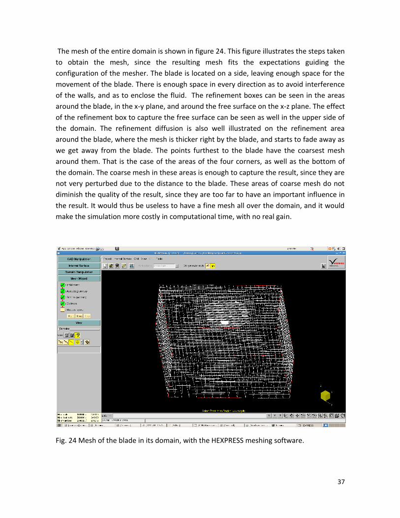
The mesh of the entire domain is shown in figure 24. This figure illustrates the steps taken

to obtain the mesh, since the resulting mesh fits the expectations guiding the

configuration of the mesher. The blade is located on a side, leaving enough space for the

movement of the blade. There is enough space in every direction as to avoid interference

of the walls, and as to enclose the fluid. The refinement boxes can be seen in the areas

around the blade, in the x-y plane, and around the free surface on the x-z plane. The effect

of the refinement box to capture the free surface can be seen as well in the upper side of

the domain. The refinement diffusion is also well illustrated on the refinement area

around the blade, where the mesh is thicker right by the blade, and starts to fade away as

we get away from the blade. The points furthest to the blade have the coarsest mesh

around them. That is the case of the areas of the four corners, as well as the bottom of

the domain. The coarse mesh in these areas is enough to capture the result, since they are

not very perturbed due to the distance to the blade. These areas of coarse mesh do not

diminish the quality of the result, since they are too far to have an important influence in

the result. It would thus be useless to have a fine mesh all over the domain, and it would

make the simulation more costly in computational time, with no real gain.

Fig. 24 Mesh of the blade in its domain, with the HEXPRESS meshing software.

38

4.2 Configuration of the Simulation.

The configuration of the simulation entails establishing the physics of the problem, and all

the hypothesis that enable us to represent and solve the problem. There are many

important considerations in this stage, some of them because of the actual physics of the

problem, and some others due to limitations of the methods or the software.

4.2.1 Positioning the domain.

The two hundred and forty nine thousand-cell mesh was imported to the Isis CFD solver.

Once in the flow solver, first of all the mesh had to be reoriented and repositioned. We

have to give the initial cardan angles to the solver, so that it knows the initial position and

orientation, since it was in this position that the imposed motion was calculated. Now,

again the whole domain will be manipulated to place it in its initial position. It is very

important not to modify the position and orientation of the system from the one

considered when calculating the model of motion, since the input motion would not be

valid for a different configuration.

The reference configuration for the blade was in a position and orientation that does not

match any time instant of the movement of the blade. The result is that if the simulation is

started on this position, there will be a leap in the first time instant, which causes

divergence of the initial solution. It is thus a reasonable choice to place the blade in the

position it has at time instant t=0s.

The translation of the blade for the flow solver is obtained by subtracting the reference

position from the position coordinates at t=0s,

[0.9289, 2.0105, 0.2478]-[1.53, 0.838, 0.375]=[-0.6011, 1.1725, -0.1272] (30)

The first coordinates signal the position of the point where the shaft joins the blade at

t=0s taken from the enhanced model of motion files. The second position gives the

coordinates of the same point that were originally used to create the mesh.

Now that the reference point is in its right position, we can reorient it so that it matches

the input orientation files. The orientation axis and angle was obtained with MATLAB,

using quaternion operations to obtain a resulting axis and angle of rotation, that is:

[-0.1523, 0.3083, 0.9390] at an angle of 53.9087:.

These resulting axis and angle were obtained from the cardan angle decomposition of the

angles at t=0s, that are 51.011605° for the yaw, 17.931464° for the pitch, and -0.246478°

39

for the roll. The pitch angle is an exception, since it is both the initial angle from the

motion files, plus the 13.08° realignment that was performed previously to the blade.

Another option for the position of the blade and its domain that avoids divergence is to

keep the domain horizontal, and to refine the free surface mesh, and then with that

refined mesh, to start the final computation.

4.2.2 Configuration of the flow solver parameters.

Now that the domain was repositioned and reoriented, the simulation can be configured.

The configuration of the simulation includes the physics of the problem, but also numeric

considerations to solve the system. The configuration will be presented and explained in

the same order as the software presents them.

First of all we are dealing with two fluids, water and air. The mathematical model or

regime is treated as laminar, so that we can obtain a solution with Isis CFD. Reference

length and velocity are now stated, at 0.45m and 3m/s, that are the length of the oar and

the final velocity of the boat. Boundary conditions are now defined as well. The sides of

the domain have a prescribed pressure, while the upper and lower lids are set to far field

conditions.

The next step is the motion definition. The input motion files of the motion shown in

chapter 3 are defined. A reference point is set at the position at t=0s. The angles of the

orientation at that same time instant for the yaw, pitch and roll are given (including the

13.08: that the blade was rotated). The mesh motion is defined as rigid motion, to avoid

problems with deformed elements due to the violent perturbation of the fluid.

Now the computational control variables are set. The time step law used is adapted to

Courant number, for a maximum of 1000 time steps, and a maximum of 5 non-linear

iterations. The maximum time step is set at 0.015s, and a maximum of 5 cycles is set for

subcycling acceleration. The size of the time step both for computational control and for

the input motion files was important, since big time steps made the simulation to abrupt

which caused its divergence. Finally the output motion variables were selected, as well as

the characteristics of the output.

On simpler test case simulations, automatic grid refinement was tested. This tool gives the

option to configure the automatic grid refinement according to a certain established logic.

The type of refinement, target grid spacing and maximum number of refinements can be

defined, as can the number of layers that will be refined, and the frequency. This

40

functionality has two main advantages, depending on how it is configured. It can give

better precision since the area of interest will always be quite refined, or it can reduce

considerably the computational time, since coarser meshes can be used together with the

automatic refinement.

4.3 Post-Processing.

Post-processing is the stage where the results are prepared to be studied and understood.

Its main objective is to try to make sense out of the results, and to present them in a

suitable way for the audience to fully understand what was done and what was achieved.

The post-processing was a big part of the project, and had different stages. To illustrate

the problem studied, an animation was done with VRML language that showed the blade

and its movement. Results were also obtained with Isis CFD that depict the blade and the

free surface around it, as well as some files containing only probes of the free surface.

The meshed blade that is used for the Isis CFD simulation is treated to change its format

into VRML format (.wrl). This format change is achieved with a FORTRAN routine

developed specifically for this animation. Developing this tool implied studying and

understanding the different meshing formats involved. This routine has a practical

application, since it can be used to provide another formatting option for the Isis CFD

software, since it was this software’s output that the program converted.

A MATLAB program was created, that receives as input the motion files for the position

and orientation in text format, and the blade mesh in VRML format, and uses them to

build a VRML animation file. This program outputs as well the new motion files for Isis

CFD, since the software uses the displacement and not the position. Another output of the

MATLAB program is the flexibility curves that were used to validate the flexibility of the

shaft.

The following four figures, 25 through 28 show the actual results of animation with VRML.

To begin with, figure 25 shows the real oar that was used. With the FORTRAN routine that

was created and the MATLAB file, we can transform the outputs of Isis CFD into an

animation with VRML even for other objects.

41

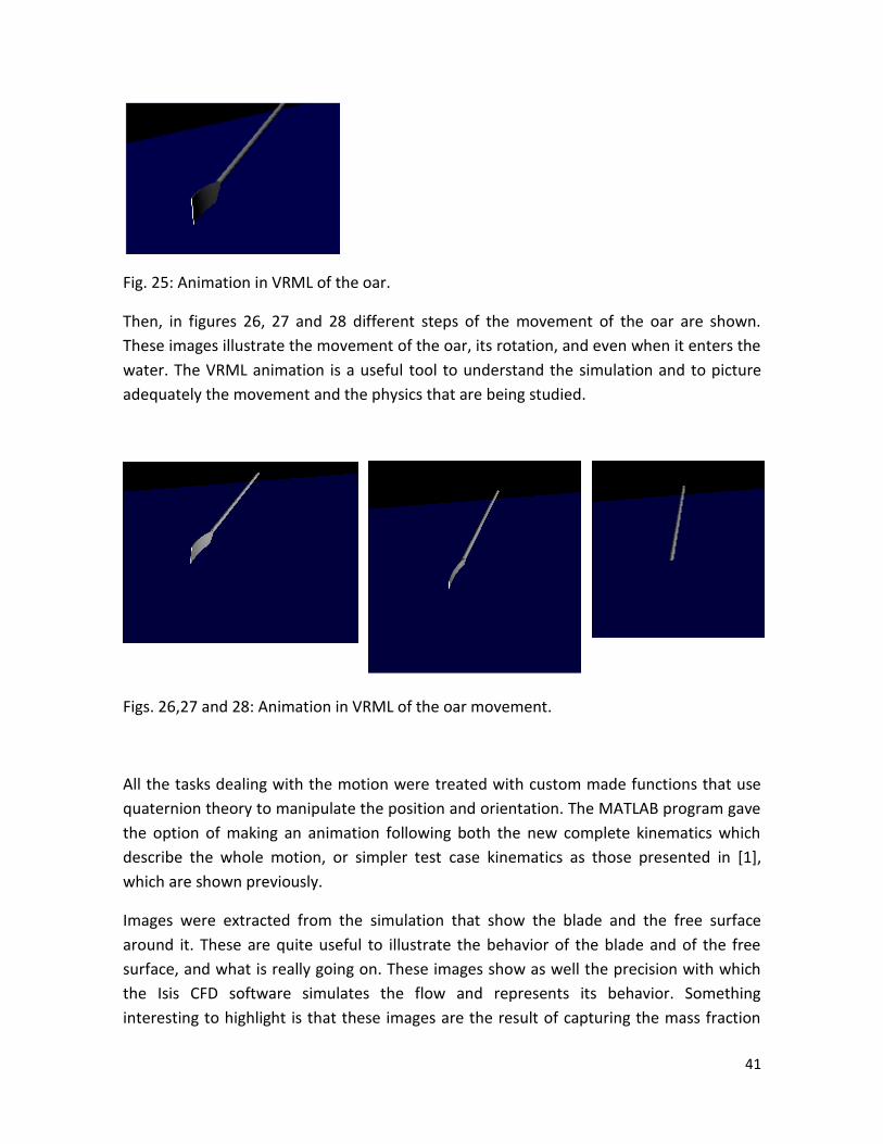
Fig. 25: Animation in VRML of the oar.

Then, in figures 26, 27 and 28 different steps of the movement of the oar are shown.

These images illustrate the movement of the oar, its rotation, and even when it enters the

water. The VRML animation is a useful tool to understand the simulation and to picture

adequately the movement and the physics that are being studied.

Figs. 26,27 and 28: Animation in VRML of the oar movement.

All the tasks dealing with the motion were treated with custom made functions that use

quaternion theory to manipulate the position and orientation. The MATLAB program gave

the option of making an animation following both the new complete kinematics which

describe the whole motion, or simpler test case kinematics as those presented in [1],

which are shown previously.

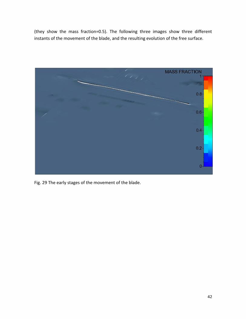
Images were extracted from the simulation that show the blade and the free surface

around it. These are quite useful to illustrate the behavior of the blade and of the free

surface, and what is really going on. These images show as well the precision with which

the Isis CFD software simulates the flow and represents its behavior. Something

interesting to highlight is that these images are the result of capturing the mass fraction

42

(they show the mass fraction=0.5). The following three images show three different

instants of the movement of the blade, and the resulting evolution of the free surface.

Fig. 29 The early stages of the movement of the blade.

43

Fig. 30 Oar blade and the free surface around it.

Fig. 31 Oar blade and the free surface around it when the blade starts turning.

44

The first image shows an early stage of movement in which the blade is still in a direction

parallel to the flow, which does not cause very turbulent flow. As the time passes, the

blade starts to rotate away from the direction of the flow, which causes a more violent

free surface motion, as can be seen first in figure 30 and then more clearly in figure 31

when the blade is already turning.

Finally to obtain the images from Isis CFD that render the free surface, again there was

some treatment of the files. First of all the simulation was run in four blocks (processors),

so the image files were divided as well in four. The first step to acquire the images was to

put them together with an existing python routine. A small tool that automatically put

together the four blocks for all the free surface probes was developed. The main objective

was to include in the VRML animation these images, but it was not possible since that

requires further programming but now in java, and because of time limitations. This

remains an objective for further work.

45

5. Results and Discussion.

The project aimed at obtaining an improved simulation that better represented the

physics of the blade rowing system. The proposed improvements were considering the

flexibility of the blade, using a realistic blade, and introducing a new model of motion that

described the full movement of the blade. Automatic grid refinement would be tested as

well.

A method for considering the flexibility of the blade was proposed and implemented. The

equations to obtain it are presented; the flexibility law was programmed in FORTRAN,

implemented in Isis CFD, and then validated in a simple test case comparing it to results

obtained independently with MATLAB. The resulting graphs presented previously in the

report show an exact match between the results obtained with Isis CFD and MATLAB.

Considering this, it can be said that the objective was achieved.

A realistic blade should be introduced. A real full scale blade was scanned and numerised.

The data obtained was treated to obtain a CAD model that could be fed to the meshing

software. The resulting blade solid was input to the meshing software, and afterwards to

the flow solver. We can thus conclude that the objective was fulfilled.

A new model of motion that described the full movement of the blade should be

considered. Input files developed by the fluid mechanics team of the Ecole Centrale

Nantes were treated and used as input. These files represent the whole movement

appropriately, and include realistic physical considerations. This objective is then achieved

as well.

Automatic grid refinement should be tested. Automatic grid refinement was included in

some of the simpler computations, but not in the last more complete ones.

Further contributions were made, additional to the main objectives of the project.

MATLAB and FORTRAN tools for pre and post processing were developed. Ranging from

small tools to change the format of input files (mesh format), to building animation files,

these tools will be useful for further work on the project.

Future work can be envisaged for the VRML animation to include the free surface probes

in the animation (requires java programming, and it was out of the scope of the project).

The automatic grid refinement should be further tested to illustrate the benefits it

represents. The reason for divergence of the solution can be studied.

46

Bibliography:

[1] Experimental and numerical investigations of the flow around an oar blade. A. Leroyer, S. Barré,.... Journal of Marine Science and Technology, vol 13, p1-15 (2008) [2] Influence of free surface, unsteadiness and viscous effects on oar blade hydrodynamic loads A. Leroyer, J-M. Kobus, S. Barré and M. Visonneau Journal of Sport Sciences (accepted)

[3] Etude du couplage écoulement/movement pour des corps solides ou à déformation

imposée par résolution des équations de Navier-Stokes. Contribution à la modélisation

numérique de la cavitation. Alban Leroyer. 20/12/2004.

[4] Note sur l’utilisation des angles de Cardan. FINE-MARINE 2.1, 25 février 2009.

[5] Back-splash in rowing-shell propulsion. M.N. Macrossan and N.W. Macrossan. June 6

2006.

[6]Rapport Déformation de l’aviron dynamométrique bâbord 556, Aviron de couple

Concept2: palette lisse à lèvre.

[7] Mécanique des milieu continus. Nicolas Moës. Course notes.

[8] Note on the “time-splitting” of the fraction volume equation in FINE/MARINE.

23/02/09

[9] New algorithms to speed up RANSE computations in hydrodynamics. Alban Leroyer et

al. 2009

[10] Quaternions and Rotations in 3-Space: How it Works. Vernon Chi. 25/09/1998

[11] Rotations using Quaternions.

[12] Refinement implementation in FINE/Marine GUI. Jeroen Wackers. 25/06/2009.

[13] Résultats expérimentaux sur palette plate en vue de réaliser des calculs numériques.

47

Appendix 1:

The MATLAB program has the following files:

oarVrmlIsis.m (main file)

lineCount.m

psi.m

theta.m

phi.m

vit.m

quatProd.m

rotaciones.m

qtoAA.m

qPass.m

resDisp.m

otherFlexibility2.m

input4Isis.m

quatMult.m

quatMult2.m

quatMult3.m

grafOutputs.m

parabolicJuntion.m

that are all thoroughly commented so that their purpose and their logic can be easily

understood and followed.

It uses as input 6 motion text files: position in x,y, and z directions, as well as the yaw,

pitch and roll angles. It has as well an input mesh file in VRML format.

48

Its outputs are files containing the three components of displacement, as well as the three

cardan angles describing the orientation. An output animation file is also created in VRML

file.