CFD Modelling of Laminar, Open-Channel Flows of Non ... · CFD Modelling of Laminar, Open-Channel...

CFD Modelling of Laminar, Open-Channel Flows of Non-Newtonian Slurries

by

César Montilla Pérez

A thesis submitted in partial fulfillment of the requirements for the degree of

Master of Science

in

Chemical Engineering

Department of Chemical and Materials Engineering University of Alberta

© César Montilla Pérez, 2017

ii

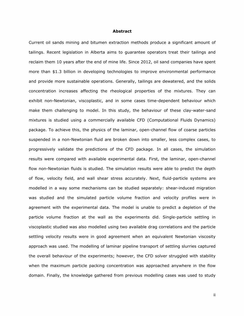
Abstract

Current oil sands mining and bitumen extraction methods produce a significant amount of

tailings. Recent legislation in Alberta aims to guarantee operators treat their tailings and

reclaim them 10 years after the end of mine life. Since 2012, oil sand companies have spent

more than $1.3 billion in developing technologies to improve environmental performance

and provide more sustainable operations. Generally, tailings are dewatered, and the solids

concentration increases affecting the rheological properties of the mixtures. They can

exhibit non-Newtonian, viscoplastic, and in some cases time-dependent behaviour which

make them challenging to model. In this study, the behaviour of these clay-water-sand

mixtures is studied using a commercially available CFD (Computational Fluids Dynamics)

package. To achieve this, the physics of the laminar, open-channel flow of coarse particles

suspended in a non-Newtonian fluid are broken down into smaller, less complex cases, to

progressively validate the predictions of the CFD package. In all cases, the simulation

results were compared with available experimental data. First, the laminar, open-channel

flow non-Newtonian fluids is studied. The simulation results were able to predict the depth

of flow, velocity field, and wall shear stress accurately. Next, fluid-particle systems are

modelled in a way some mechanisms can be studied separately: shear-induced migration

was studied and the simulated particle volume fraction and velocity profiles were in

agreement with the experimental data. The model is unable to predict a depletion of the

particle volume fraction at the wall as the experiments did. Single-particle settling in

viscoplastic studied was also modelled using two available drag correlations and the particle

settling velocity results were in good agreement when an equivalent Newtonian viscosity

approach was used. The modelling of laminar pipeline transport of settling slurries captured

the overall behaviour of the experiments; however, the CFD solver struggled with stability

when the maximum particle packing concentration was approached anywhere in the flow

domain. Finally, the knowledge gathered from previous modelling cases was used to study

iii

the laminar, open-channel flow of coarse particles in non-Newtonian suspension. The model

developed in this study was able to predict the settling of coarse particles when compared

with experimental data. It was found that particles settle predominantly in the sheared zone

where they form a stationary bed, as also indicated by the velocity profiles. In addition, a

parametric study was performed to determine which flow parameters and rheological

properties have a significant impact on the transport of coarse particles suspended in a non-

Newtonian carrier fluid. The simulation results showed that the flow rate, mixture density,

and bulk particle volume fraction are the most impactful parameters in hindering coarse

particle settling. The variation of the mixture yield stress had no significant effect on coarse

particle settling. An increase in particle diameter had an increasing effect on particle

settling. Replacing the semi-circular channel geometry by an equivalent rectangular channel

increased the size the depth the settled bed. The model presented in this study can be used

to evaluate multiple conditions and for scaling purposes, or to enable the selection of a

limited experimental matrix.

iv

Acknowledgements

I would like to express my gratitude to my supervisor, Dr. Sean Sanders, for giving me the

opportunity of being part of the Pipeline Transport Processes research group, and for

guiding me throughout this research project.

Special thanks to Terry for her invaluable support during the project. I would also like to

thank my fellow group members for all the insightful conversations.

My sincerest gratitude goes to Diego, friends, and family for their invaluable support along

this journey.

This research was conducted through the support of the Institute for Oil Sands Innovation

(IOSI) and the NSERC Industrial Research Chair in Pipeline Transport Processes (RSS). The

contributions of Canada’s Natural Sciences and Engineering Research Council (NSERC) and

the Industrial Sponsors (Canadian Natural Resources Limited, CNOOC-Nexen Inc.,

Saskatchewan Research Council’s Pipe Flow Technology CentreTM, Shell Canada Energy,

Suncor Energy, Syncrude Canada Ltd., Total SA, Teck Resources Ltd., and Paterson & Cooke

Consulting Engineering Ltd.) are also recognized with gratitude

v

Table of Contents

1. Introduction ...................................................................................................... 1

1.1 Oil sands overview ....................................................................................... 1

1.2 Research context and objectives .................................................................... 2

1.3 Thesis contents ........................................................................................... 6

1.4 Contributions .............................................................................................. 6

2. Literature review ............................................................................................... 8

2.1 Introduction ................................................................................................ 8

2.2 Fluid behaviour classification ......................................................................... 8

2.2.1 Non-Newtonian fluids ................................................................................ 9

2.3 Open-channel flow ..................................................................................... 10

2.3.1 Sheet flow of viscoplastic fluids ................................................................. 10

2.3.2 Friction losses on laminar, open-channel, flow of non-Newtonian fluids ........... 12

2.4 Fluid-particle systems ................................................................................. 15

2.4.1 Single-particle systems ............................................................................ 16

2.4.2 Multi-particle systems .............................................................................. 22

2.5 Numerical modelling ................................................................................... 27

2.5.1 Numerical modelling of viscoplastic fluids ................................................... 27

2.5.2 Numerical modelling of coarse particle suspensions ...................................... 28

2.6 STAR-CCM+: Overview ............................................................................... 29

2.6.1 Meshing capabilities ................................................................................ 29

2.6.2 Multiphase flow modelling ........................................................................ 32

2.6.3 Non-Newtonian flow modelling .................................................................. 35

2.6.4 Solution Analysis .................................................................................... 35

3. Homogeneous, laminar, open-channel flow of non-Newtonian fluids ........................ 37

3.1 Semi-circular channel ................................................................................. 37

3.1.1 Model validation ..................................................................................... 41

3.2 Rectangular channel ................................................................................... 50

vi


3.3 Modelling limitations ................................................................................... 54

3.4 Conclusions ............................................................................................... 55

3.5 Recommendations ...................................................................................... 56

4. Fluid-particle systems – preliminary studies ......................................................... 57

4.1 Shear-induced migration ............................................................................. 57


4.2 Single-particle settling in viscoplastic fluids .................................................... 65


4.3 Laminar transport of coarse particles ............................................................ 70


4.4 Modelling limitations ................................................................................... 75

4.5 Conclusions ............................................................................................... 75

4.6 Recommendations ...................................................................................... 76

5. Laminar, open-channel flow of thickened tailings .................................................. 77

5.1 Model validation......................................................................................... 79

5.2 Parametric analysis .................................................................................... 85

5.3 Limitations ................................................................................................ 98

5.4 Conclusions ............................................................................................... 99

5.5 Recommendations ..................................................................................... 100

6. Conclusions and recommendations for future work .............................................. 101

6.1 Summary and conclusions .......................................................................... 101

6.2 Recommendations for future work ............................................................... 102

References ........................................................................................................... 104

APPENDIX A: SOFTWARE AND HARDWARE TECHNICAL SPECIFICATIONS ...................... 113

APPENDIX B: SIMULATION DATA ............................................................................. 116

vii

List of Figures

Figure 1.1: Tailings pond schematic5. .......................................................................... 1

Figure 1.2: Types of fluid flow behaviour (reproduced)20. ............................................... 3

Figure 1.3: A high-level summary of a tailings disposal design strategy4 .......................... 4

Figure 2.1: Schematic representation of unidirectional shearing flow20. ............................ 9

Figure 2.2: Flow configuration for sheet flow reproduced from De Kee et al.44 ................. 11

Figure 2.3: Moody diagram showing the relationship between the Fanning friction factor and

the Reynold number defined by Equation (2.21), with ReH defined by Equation (2.17) ..... 15

Figure 2.4: Schematic representation of forces acting on a falling solid sphere ................ 17

Figure 2.5: Shape of the sheared envelope surroinding a sphere in creeping motion through

viscoplastic fluids: (a) Ansley and Smith67, (b) Yoshioka et al68., (c) Beris et al.62 from61. 19

Figure 2.6: Relative fall velocity versus Reynolds number70 with 𝜏𝑟𝑒𝑓 = 0.3𝜏 .................... 21

Figure 2.7: Equation (2.39) prediction using experimental data from Valentik and

Whitmore74, Ansley and Smith67, Wilson et al.70, Tran et al.75, and Shokrollahzadeh35. ..... 22

Figure 2.8: Prism layer mesher example, with (a) Progressive layer stretching and (b)

Constant stretching ................................................................................................ 30

Figure 2.9: (a) Source, (b) target, and (c) guide surfaces for directed meshing ............... 31

Figure 2.10: Directed mesh example ........................................................................ 31

Figure 2.11: Example of derived parts created using STAR-CCM+: a plane and a vertical

centerline inside a cylinder ...................................................................................... 36

Figure 3.1: Saskatchewan Research Council’s 156.7 mm flume circuit used by Spelay17 ... 37

Figure 3.2: Mesh structure for the semi-circular channel simulations ............................. 38

Figure 3.3: Maximum CFL number monitor extracted from STAR-CCM+ for Case 1A ........ 40

Figure 3.4: Example of residuals plot for Case 4A ....................................................... 41

Figure 3.5: Contour plot of the volume fraction of mixture for case 1A in a plane

perpendicular to the flow direction ............................................................................ 43

Figure 3.6: Parity plot for experimental and predicted depth of flow for the conditions shown

in Table 3.3. .......................................................................................................... 43


in Table 3.3. .......................................................................................................... 44

Figure 3.8: Wall stress distribution for Case 2B (experimental conditions shown in Table 3.3)

........................................................................................................................... 45

Figure 3.9: Parity plot for experimental and predicted wall shear stress for the conditions

shown in Table 3.3. ................................................................................................ 45

viii

Figure 3.10: Parity plot for experimental and predicted average velocity for the conditions

shown in Table 3.3. ................................................................................................ 46

Figure 3.11: Normalized centerline velocity profile comparison between experiments by

Spelay and simulation results for Case 2A. ................................................................ 47


Spelay and simulation results for Case 2B. ................................................................ 47


Spelay and simulation results for Case 2G. ................................................................ 48

Figure 3.14: Comparison of the simulation results and Fanning friction factor correlation by

Burger et al.53 ....................................................................................................... 49

Figure 3.15: Schematic of rectangular flume used by Haldenwang et al.45 ...................... 50

Figure 3.16: Mesh structure for the rectangular channel simulations .............................. 51

Figure 3.17: Comparison of the normalized centerline velocity profile between simulations

and the laminar sheet flow model44 for Case 3A .......................................................... 52


and the laminar sheet flow model44 for Case 3B .......................................................... 53


and the laminar sheet flow model44 for Case 4A .......................................................... 54


and the laminar sheet flow model44 for Case 4B. ......................................................... 54

Figure 4.1: (a) Schematic of the experimental setup (b) Superconducting 1.9 T magnet29 57

Figure 4.2: Mesh structure for the shear-induced migration simulations ......................... 58

Figure 4.3: Minimum particle volume fraction monitor with respect of time for Case 5B .... 59

Figure 4.4: Contour plot of the particle volume fraction for Case 5B in a plane perpendicular

to the flow direction ............................................................................................... 60

Figure 4.5: Contour plot of the carrier fluid velocity for Case 5B in a plane perpendicular to

the flow direction ................................................................................................... 61

Figure 4.6: Developed particle volume fraction comparison between simulation results and

experiments by Hampton et al.29 for Case 5A ............................................................. 61


experiments by Hampton et al.29 for Case 5B ............................................................. 62


experiments by Hampton et al.29 for Case 5C ............................................................. 62

Figure 4.9: Developed velocity profile comparison between simulation results and

experiments by Hampton et al.29 for Case 5A ............................................................. 63

ix


experiments by Hampton et al.29 for Case 5B ............................................................. 64


experiments by Hampton et al.29 for Case 5C ............................................................. 64

Figure 4.12: Schematic representation of the settling column used by Shokrollahzadeh35 . 66

Figure 4.13: Mesh representation for single-particle settling simulations. ....................... 67

Figure 4.14: Maximum particle velocity monitor plot using STAR-CCM+ for Case 10B ...... 67

Figure 4.15: Comparison between simulation results and experiments for a particle settling

in a viscoplastic fluid. Conditions listed in Table 4.5 .................................................... 69

Figure 4.16: Comparison between simulation results and the Newtonian drag curve ........ 70

Figure 4.17: The 50 mm pipeflow loop used in the experiments by Gillies et al.32 where: d)

Gamma ray densitometer, g) Glass observation section, h) Heat Exchanger, a) Hot film

anemometer, s) Sampler, T) Temperature sensor, V) Acrylic observation section ............ 70

Figure 4.18: Mesh structure used in the laminar transport of coarse particles simulations . 71

Figure 4.19: Particle volume fraction profile between simulation results and experiments by

Gillies et al.32 for Case 11A ...................................................................................... 72


Gillies et al.32 for Case 11B ...................................................................................... 73

Figure 4.21: Simulated velocity profiles for Cases 11A and 11B .................................... 74

Figure 5.1: Mesh structure used for thickened tailings simulations ................................ 77

Figure 5.2: Contour plot for particle volume fraction, 14.5 m away from the channel inlet,

perpendicular to the flow, for Case 12B ..................................................................... 80

Figure 5.3: Contour plot for mixture velocity magnitude 14.5 m away from the channel inlet,

perpendicular to the flow, for Case 12B ..................................................................... 80

Figure 5.4: Chord-averaged particle volume fraction comparison between simulation results

and experiments by Spelay17 for Case 12A ................................................................ 81


and experiments by Spelay17 for Case 12B ................................................................ 81


and experiments by Spelay17 for Case 12C ................................................................ 82


and experiments by Spelay17 for Case 12D ................................................................ 82

Figure 5.8: Simulated centerline velocity profile for the carrier fluid, 14.5 m away from the

channel inlet, for Case 12B ...................................................................................... 83

Figure 5.9: Particle volume fraction variation with time for case 10B ............................. 84

x

Figure 5.10: Simulated maximum particle volume fraction variation with distance from the

inlet ..................................................................................................................... 85

Figure 5.11: Simulated maximum wall shear stress variation with distance from the inlet . 85

Figure 5.12: Chord-averaged particle volume fraction variation with carrier fluid yield stress

........................................................................................................................... 86

Figure 5.13: Predicted carrier fluid centerline velocity profile with varying carrier fluid yield

stress ................................................................................................................... 87

Figure 5.14: Chord-averaged particle volume fraction profile with varying channel diameter

and depth of flow ................................................................................................... 88

Figure 5.15: Predicted carrier fluid centerline velocity profile with varying channel diameter

and depth of flow ................................................................................................... 88


and constant depth of flow ...................................................................................... 89


and constant depth of flow ...................................................................................... 89

Figure 5.18: Chord-averaged particle volume fraction profile in a semi-circular and

rectangular channel ................................................................................................ 90

Figure 5.19: Predicted carrier fluid centerline velocity profile in a semi-circular and

rectangular channel ................................................................................................ 90

Figure 5.20: Contour plot for velocity of the particle phase 14.5 m away from the channel

inlet in: (a) Semi-circular channel and (b) rectangular channel ..................................... 91

Figure 5.21: Contour plot for shear stress 14.5 m away from the channel inlet in: (a) Semi-

circular channel and (b) rectangular channel .............................................................. 92

Figure 5.22: Chord-averaged particle volume fraction with varying particle diameter ....... 93

Figure 5.23: Predicted carrier fluid centerline velocity profile with varying particle diameter

........................................................................................................................... 93

Figure 5.24: Chord-averaged particle volume fraction with varying particle volume fraction

........................................................................................................................... 94

Figure 5.25: Relative particle volume fraction profiles with varying inlet particle volume

fraction ................................................................................................................ 94

Figure 5.26: Carrier fluid velocity profiles with varying inlet particle volume fraction ........ 95

Figure 5.27: Chord-averaged particle volume fraction with varying carrier fluid density .... 95

Figure 5.28: Predicted carrier fluid centerline velocity profile with varying carrier fluid

density ................................................................................................................. 96

Figure 5.29: Chord averaged particle volume fraction profile with varying flow rate ......... 97

xi

Figure 5.30: Normalized centerline velocity profile with varying flow rate ....................... 97

xii

List of Tables

Table 1.1: Tailings management technologies used in current oil sands mining projects ..... 2

Table 2.1: Drag coefficient correlations based on the particle’s Reynolds number ............ 16

Table 3.1: STAR-CCM+ models used on the semi-circular channel simulations ................ 39

Table 3.2: Rheological properties of the mixtures modelled in this study17 ...................... 41

Table 3.3: Experimental conditions considered for modelling in the semi-circular channel

reported by Spelay17 .............................................................................................. 42

Table 3.4: Rheological properties of the fluids evaluated by Haldenwang et al.45 ............. 51

Table 3.5: Experimental conditions considered for modelling in the rectangular channel

reported by Haldenwang et al.45 ............................................................................... 51

Table 4.1: STAR-CCM+ models used in the modelling of shear-induced migration ........... 58

Table 4.2: Experimental conditions modelled for shear-induced migration29 .................... 60

Table 4.3: Experimental entrance length and simulated average wall shear stress for cases

in Table 4.2 ........................................................................................................... 65

Table 4.4: STAR-CCM+ models used in the single-particle settling simulations ................ 66

Table 4.5: Experimental conditions used in the particle settling simulations of the present

study35 ................................................................................................................. 68

Table 4.6: Modelling approaches for a solid sphere settling in a viscoplastic fluid. ............ 68

Table 4.7: Experimental conditions modelled for the laminar transport of settling slurries . 72

Table 5.1: STAR-CCM+ models used to model thickened tailings ................................... 78

Table 5.2: Mixture and particle properties used in the modelling of the laminar, open-

channel flow of thickened tailings17 ........................................................................... 79

Table 5.3: Experimental conditions modelled in the transport of coarse particle suspended in

a viscoplastic fluid. ................................................................................................. 79

xiii

List of Symbols

Symbol Description Units

A Area m2

a Geometrical parameter for the Kozicki and Tiu model -

a Numerical constant for the Blasius equation -

a Particle radius m

𝑎𝑇 Temperature factor (Equation 2.68) -

𝐵𝑖𝐻𝐵 Bingham number -

b Geometrical parameter for the Kozicki and Tiu model -

b Numerical constant for the Blasius equation -

𝐶𝐷 Drag coefficient -

𝐶2 Quadratic coefficient (Equation 2.44) -

c Numerical constant for the Blasius equation -

d Numerical constant for the Blasius equation -

d Particle diameter m

e Fitting parameter (Equation 2.18) -

𝐹1 Power law relationship for laminar flows -

𝐹2 Power law relationship for turbulent flows -

F𝐵 Buoyancy force N

F𝐷 Drag force N

F𝐺 Gravity force N

(𝐅𝑖𝑛𝑡)𝑖 Internal forces of the ith phase (Equation 2.65) N

𝑭𝑠 Surface forces acting on the particle N

𝑭𝑏 Body forces acting on the particle N

𝑓(𝜙) Hindrance function -

𝑓𝑁𝑒𝑤𝑡𝑜𝑛𝑖𝑎𝑛(𝜙) Hindrance function for a Newtonian fluid -

𝑓 Fanning friction factor -

g Gravity force vector m/s2

g Gravity force magnitude m/s2

h Depth of flow m

j Fitting parameter (Equation 2.18) -

𝐾𝑠 Contact contribution (Equation 2.47) -

𝐾𝑠 Sedimentation flux coefficient (Equation 2.57) kg/m3

xiv

K Numerical constant dependent of channel shape -

𝐾𝑐 Proportional constant (Equation 2.53) -

𝐾 Proportional constant (Equation 2.54) -

𝐾𝑛 Contact contribution (Equation 2.55) -

k Consistency index Pa.sn

𝑘𝑟 Relative consistency index -

𝑚𝑖𝑗 Mass transfer rate to phase i, from phase j (𝑚𝑖𝑗 ≥ 0). kg/s

𝑚𝑗𝑖 Mass transfer rate to phase j, from phase i (𝑚𝑗𝑖 ≥ 0). kg/s

𝑚𝑝 Particle mass kg

𝑁𝑠 Flux due to sedimentation (Equation 2.57) m/s

𝑁𝑐 Flux due to spatially varying interaction (Equation 2.53) m/s

𝑁 Flux due to spatially varying viscosity (Equation 2.54) m/s

n Power law exponent -

𝑛𝑟 Relative power law exponent -

p Pressure Pa

𝑄∗ Modified dynamic parameter -

𝑅𝑒 Reynolds number -

𝑅𝑒∗ Shear Reynolds number -

𝑅𝑒𝐵∗ Reynolds number for Bingham fluids in open-channel flow -

𝑅𝑒𝐵 Abulnaga’s Reynolds number -

𝑅𝑒𝐻 Haldenwang et al. Reynolds number -

𝑅𝑒𝑝 Particle Reynolds number -

𝑅𝑒𝑃𝐿 Reynolds number for power law fluids -

𝑅𝑒𝑝∗ Reynolds number for power law fluids in open-channel flow -

𝑅𝑒𝑍ℎ𝑎𝑛𝑔 Zhang’s Reynolds number -

𝑅ℎ Hydraulic radius m

𝑠𝑖𝛼 Phase mass source term (Equation 2.66) kg/m3

𝑠𝑖𝑉 Phase momentum source term (Equation 2.65) kg*m/s

t Fitting parameter (Equation 2.18) -

�̅� Average velocity m/s

𝑉∞ Particle terminal velocity m/s

𝑉∞,𝑠 Hindered particle settling velocity m/s

xv

𝑉∗ Shear velocity m/s

𝑉𝑥 Velocity component in the X direction m/s

𝑉𝑦< Velocity component in the Y direction in the plug m/s

𝑉𝑦> Velocity component in the Y direction in the sheared zone m/s

𝐯𝑔 Grid velocity (Equation 2.64) m/s

𝒗𝒑 Particle velocity m/s

X(n) Deviation factor -

x0 Distance between the free surface and the yielding transition

surface m

𝑌𝐺 Static equilibrium parameter -

Greek symbols

Symbol Description Units

𝛼 Channel slope with respect of the horizontal degrees

𝛼 Rheogram shape factor (Equation 2.39) -

𝛼 Drag force constant (Equation 2.60) -

𝛼𝐵 Rheogram shape factor calculated from the Bingham model -

�̇� Shear rate s-1

�̇��̅�(𝜙) Average local shear rate (Equation 2.60) s-1

𝑟 Relative viscosity -

𝑠 Viscosity of the suspension Pa.s

𝑐 Viscosity of the carrier fluid Pa.s

[] Krieger and Dougherty exponent -

𝜇 Newtonian viscosity Pa.s

𝜇𝑎𝑝𝑝 Apparent viscosity Pa.s

𝜇𝑒𝑞 Equivalent viscosity Pa.s

𝜇𝑖 Dynamic viscosity of the ith phase Pa.s

𝜇0 Yielding viscosity Pa.s

𝜇𝑝 Bingham plastic viscosity Pa.s

𝜉 Relative shear stress -

𝜌 Density kg/m3

xvi

𝜌𝑖 Density of the ith phase kg/m3

𝜌𝑠 Particle density kg/m3

𝜌𝑓 Fluid density kg/m3

𝜏 Shear Stress Pa

𝜏̅ Mean surficial stress (Equation 2.36) Pa

𝜏𝑖 Molecular stress (Equation 2.65) Pa

𝜏𝑖𝑡 Turbulent stress (Equation 2.65) Pa

𝜏𝑟𝑒𝑓 Reference shear stress Pa

𝜏𝑤 Wall shear stress Pa

𝜏𝑥𝑦 Shear stress at any point X on a surface parallel to Y-axis Pa

𝜏𝑦 Yield stress Pa

𝜏𝑦𝐵 Bingham yield stress Pa

𝜏𝑦𝐻 Herschel-Bulkley yield stress Pa

𝜏𝑦𝑟 Relative yield stress -

𝜙 Particle volume fraction -

𝜙𝑚𝑎𝑥 Particle maximum packing volume fraction -

𝜒 Yield stress to wall shear stress ratio -

𝜒 Void fraction -

1

1. Introduction

1.1 Oil sands overview

Every mining operation in the world produces tailings. This is particularly important in the

process of mining oil sand and extracting bitumen for upgrading to synthetic crude oil, as

significant volumes of fluid fine tailings are produced. For instance, historical production

rates of 1 million barrels of oil per day1,2 result in approximately 0.3 million m3 tailings

produced per day3. These mixtures are composed of water, clay, sand, and some residual

bitumen. Without going into details of any specific mining operation, a generalized

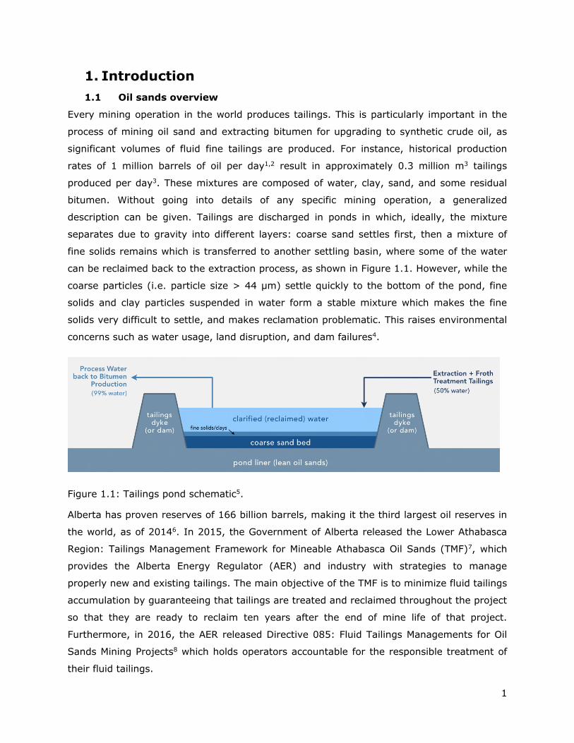
description can be given. Tailings are discharged in ponds in which, ideally, the mixture

separates due to gravity into different layers: coarse sand settles first, then a mixture of

fine solids remains which is transferred to another settling basin, where some of the water

can be reclaimed back to the extraction process, as shown in Figure 1.1. However, while the

coarse particles (i.e. particle size > 44 μm) settle quickly to the bottom of the pond, fine

solids and clay particles suspended in water form a stable mixture which makes the fine

solids very difficult to settle, and makes reclamation problematic. This raises environmental

concerns such as water usage, land disruption, and dam failures4.

Figure 1.1: Tailings pond schematic5.

Alberta has proven reserves of 166 billion barrels, making it the third largest oil reserves in

the world, as of 20146. In 2015, the Government of Alberta released the Lower Athabasca

Region: Tailings Management Framework for Mineable Athabasca Oil Sands (TMF)7, which

provides the Alberta Energy Regulator (AER) and industry with strategies to manage

properly new and existing tailings. The main objective of the TMF is to minimize fluid tailings

accumulation by guaranteeing that tailings are treated and reclaimed throughout the project

so that they are ready to reclaim ten years after the end of mine life of that project.

Furthermore, in 2016, the AER released Directive 085: Fluid Tailings Managements for Oil

Sands Mining Projects8 which holds operators accountable for the responsible treatment of

their fluid tailings.

2

Since 2012, oil sand companies have spent more than $1.3 billion in developing

technologies to improve environmental performance and provide more sustainable

operations focusing in 4 major areas: greenhouse gases, water, land, and tailings9. In the

management of tailings, most projects are focused on accelerated dewatering as it leads to

more efficient process water recycling (and thus reduced fresh water consumption) and

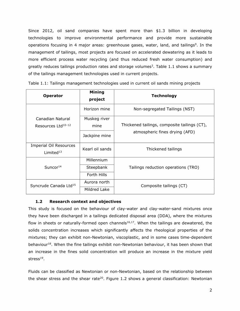
greatly reduces tailings production rates and storage volumes3. Table 1.1 shows a summary

of the tailings management technologies used in current projects.

Table 1.1: Tailings management technologies used in current oil sands mining projects

Operator Mining

project Technology

Canadian Natural

Resources Ltd10–12

Horizon mine Non-segregated Tailings (NST)

Muskeg river

mine Thickened tailings, composite tailings (CT),

atmospheric fines drying (AFD) Jackpine mine

Imperial Oil Resources

Limited13 Kearl oil sands Thickened tailings

Suncor14

Millennium

Tailings reduction operations (TRO) Steepbank

Forth Hills

Syncrude Canada Ltd15 Aurora north

Composite tailings (CT) Mildred Lake

1.2 Research context and objectives

This study is focused on the behaviour of clay-water and clay-water-sand mixtures once

they have been discharged in a tailings dedicated disposal area (DDA), where the mixtures

flow in sheets or naturally-formed open channels16,17. When the tailings are dewatered, the

solids concentration increases which significantly affects the rheological properties of the

mixtures; they can exhibit non-Newtonian, viscoplastic, and in some cases time-dependent

behaviour18. When the fine tailings exhibit non-Newtonian behaviour, it has been shown that

an increase in the fines solid concentration will produce an increase in the mixture yield

stress19.

Fluids can be classified as Newtonian or non-Newtonian, based on the relationship between

the shear stress and the shear rate20. Figure 1.2 shows a general classification: Newtonian

3

fluids are characterized by a linear relationship between shear stress and shear rate, where

the slope of the line is defined as the Newtonian viscosity of the fluid. Non-Newtonian fluids

usually show a non-linear relationship and can be further classified as dilatant, pseudo-

plastic, or viscoplastic, the latter being characterized by the presence of a yield stress,

defined as stress required for the material to flow. Below this threshold, the material will

behave as an elastic solid. There are several mathematical models to describe the non-

Newtonian flow behaviour and they will be explained in more detail in Chapter 2.

Figure 1.2: Types of fluid flow behaviour (reproduced)20.

Typically, the design of the tailings disposal system begins with the design of a thickener,

which provides an overflow that can be reused in the process. The underflow or dewatered

tailings, exhibit non-Newtonian behaviour. Their high apparent viscosity makes it cost-

prohibitive to operate under turbulent conditions, in most cases. Thus, most dewatered

tailings lines operate under laminar flow conditions. As such, it becomes critical to

understand the underlying mechanisms involved in coarse solids transport under these

conditions17 because of the implications in the pump system design/power consumption. For

example, consider the design sequence shown in Figure 1.3, which suggests that one should

design the disposal system back-to-front; namely, selecting the disposal method first, then

the designing the pumping system, and ending with the thickener design, or the method by

which the tailings are dewatered. The rheological properties of the tailings are needed to

predict consolidation, as well as for the design of the tailings line, and the suction side of

the pump for the thickener4.

4

Figure 1.3: A high-level summary of a tailings disposal design strategy4

Advances in hardware and in Computational Fluids Dynamics (CFD) techniques have

permitted the use of CFD in many areas, such as sports, automotive, chemical and mineral

processing, civil and environmental engineering, heat transfer, power generation, among

others. Simulations can complement experiments, providing a cost-effective way to study

multiple scenarios that would be otherwise difficult, or even impossible, with experiments21.

However, modelling tailings mixtures poses many challenges because they are non-

Newtonian (usually viscoplastic), time-dependent, and contain coarse (settling)

particles17,22. One of the challenges in modelling yield stress fluid flows is to properly

represent the region where the shear stress is below the yield stress23. Methods have been

developed to overcome this and will be explained in more detail in Chapter 2.

Solid particles suspended in a fluid are known to affect the resistance of the mixture to flow,

or its suspension viscosity, which has been found to be an increasing function of the solid

particle volume fraction24. For concentrated suspensions, where the particle volume fraction

is greater than 0.15, the suspension viscosity increases rapidly with particle volume

fraction24; semi-empirical correlations have been proposed to account for this effect25–27.

Other phenomena that can be present when studying suspensions is the shear-induced

migration of solid particles because of gradients in shear rate28–30, and hindered-settling

when dealing with particles that are heavier than the suspending fluid31,32.

5

Few numerical studies have been performed to study the open-channel flow of coarse

particle, non-Newtonian suspensions. For example, Spelay17 studied the behaviour of

tailings mixtures for a variety of conditions both experimentally and numerically. He

attempted to use a commercial CFD package to model tailings mixtures, however, the CFD

packages at the time were unable to incorporate the physics of the problem properly. Thus,

he developed his own code that could predict the behaviour of laminar, open-channel flow of

tailings. Despite the model being limited to one-dimensional flow of suspensions, he could

validate the model for the laminar flow of thickened tailings successfully. Treinen and

Jacobs33 used commercial software to study particle settling and shear-induced migration in

viscoplastics fluids. Their results were able to capture overall behaviour but their predictions

differ from experimental results. Sittoni et al34 proposed a 2DV (two dimensional vertical)

numerical module, referred to as Delft3D slurry. The authors showed some promising

preliminary results but their model requires further validation.

As shown above, most numerical models are limited to one or two-dimensional studies, and

some of their results need further validation using experimental studies. Thus, the objective

of this project is to develop a reliable, three-dimensional model that can predict the flow

behaviour of non-Newtonian tailings mixtures, using a commercial CFD package. In

addition, one of the overall objectives of this work is to study the main parameters that

govern the transport of monodisperse coarse solids in these mixtures. To achieve this, the

physics of the laminar, open-channel flow of coarse particles in non-Newtonian suspensions

are broken down into smaller, less complex cases, to progressively validate the predictions

of the CFD package. The modelling is divided in the following cases: laminar, open-channel

flow non-Newtonian fluids; fluid-particle systems, which include shear-induced migration,

single-particle settling, laminar pipeline transport of settling slurries, and laminar,

heterogeneous, open-channel flow of coarse particles in non-Newtonian suspensions. Each

modelling stage is validated using available experimental data and correlations from a

variety of studies. In summary, to complete the project, the following activities were

undertaken:

Model and validate the laminar, homogeneous, open-channel flow of non-Newtonian

fluids

Model and validate the shear-induced migration of solid particles suspended in a

Newtonian carrier fluid

Model and validate the single-particle settling of a sphere through a viscoplastic fluid

Model and validate the laminar pipeline transport of coarse particles suspended in a

Newtonian fluid

6

Model and validate the laminar, heterogeneous, open-channel flow of non-Newtonian

fluids

1.3 Thesis contents

The thesis contains six chapters, including the current one. Chapter 2 provides a literature

review of the main concepts and studies relevant to the project, including an overview of

STAR-CCM+, the commercial CFD package used throughout this project.

In Chapter 3, the focus is on the open-channel flow of homogeneous, non-Newtonian fluids.

The predictions of the CFD model are tested against experimental data, using parameters

that fully describe these type of flows, i.e., depth of flow, fluid velocity and wall shear

stress. Limitations, conclusions, and recommendations specific to the application of the CFD

model to these types of flows are included at the end of the chapter.

In Chapter 4, a number of different fluid-particle systems are evaluated. Specifically, the

chapter focuses on characteristic behavior of suspensions: shear-induced migration, single-

particle settling and laminar pipeline transport of settling slurries. For this evaluation, the

following studies were considered: Hampton et al.29 studied the shear-induced migration of

solid particles suspended in a Newtonian fluid using nuclear magnetic resonance (NMR);

Shokrollahzadeh35 studied the single-particle settling of spheres through viscoplastic fluids;

and Gillies et al.32 studied the laminar pipeline transport of coarse particles suspended in a

Newtonian fluid. Limitations, conclusions, and recommendations specific to these

simulations are included at the end of the chapter.

In Chapter 5, the results from previous chapters are combined, and a model to characterize

the flow behavior of non-Newtonian suspensions under laminar, open-channel flow is

presented. This model is validated with the experimental data of Spelay17. In addition, a

parametric study is performed to determine the suspension properties and flow parameters

that have dominant effects on monodisperse coarse particle transport. At the end of the

chapter, modelling limitations, conclusions, and recommendations are shown.

Finally, Chapter 6 contains a summary and extended discussion of the main findings of this

project, an assessment of the extent to which the objectives of this project were

accomplished, and recommendations for future work.

1.4 Contributions

There are currently few numerical models that can be used to study coarse particle

transport in non-Newtonian fluids. This project presents a three-dimensional numerical

7

model, developed using a commercial CFD package, to study the behaviour of monodisperse

non-Newtonian suspensions flowing under laminar, open-channel flow conditions.

The model uses rheological properties, volume fraction of the phases, carrier fluid and solid

particle properties, as well as operating conditions as inputs. Although the model was

validated successfully using data from previous studies, the available experimental data sets

were limited to four conditions. The author therefore recommends that more experimental

studies are needed to further validate the model.

Fluid dynamics researchers can benefit from the model presented in this project by using it

to plan their experimental protocols and in identifying relevant conditions when time and

resources might be limited. The model can also help visualize flow phenomena when flow

visualization from experiments is difficult. CFD researchers can continue to expand the

modelling capabilities as advances in software and hardware become available. Design

engineers can use this model in the preliminary design of tailings disposal systems. In

addition, design and operations engineers can use the model to assess multiple conditions

and their effect on the transport of thickened tailings for their specific conditions.

8

2. Literature review

2.1 Introduction

This chapter contains a review of the most relevant literature to the primary objective of the

project; namely, to apply a commercial CFD model that can predict the behaviour of non-

Newtonian suspensions flowing under laminar, open-channel flow conditions.

First, a general summary fluid behaviour classification is presented. This will provide the

reader with a basic understanding of rheology concepts and will highlight distinct

characteristics of Newtonian and non-Newtonian fluids. In addition, the relevant constitutive

equations that can describe the behaviour of different non-Newtonian fluids are shown, as

these are critical to the mathematical modelling of the fluids and slurries described in the

thesis.

Next, open-channel flows are discussed and a model to study laminar sheet flows is

introduced, which is relevant to the results presented in Chapter 3. In addition, the friction

losses on open channels are explained, along with the definition of the Reynolds number for

non-Newtonian fluids, and how it relates to friction losses.

Subsequently, fluid-particle systems are discussed. This section is divided into single-

particle and multi-particle systems, and provide the framework to understand characteristic

phenomena of these systems. The results in Chapter 4 and 5 can be understood after this

background has been presented.

Finally, an overview of STAR-CCM+, the CFD package used in this study is given, which

provides with the terminology and models used throughout this project.

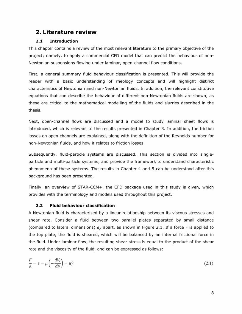
2.2 Fluid behaviour classification

A Newtonian fluid is characterized by a linear relationship between its viscous stresses and

shear rate. Consider a fluid between two parallel plates separated by small distance

(compared to lateral dimensions) 𝑑𝑦 apart, as shown in Figure 2.1. If a force F is applied to

the top plate, the fluid is sheared, which will be balanced by an internal frictional force in

the fluid. Under laminar flow, the resulting shear stress is equal to the product of the shear

rate and the viscosity of the fluid, and can be expressed as follows:

𝐹

𝐴= 𝜏 = 𝜇 (−

𝑑𝑉𝑥𝑑𝑦) = 𝜇�̇� (2.1)

9

Figure 2.1: Schematic representation of unidirectional shearing flow (reproduced)20.

The constant of proportionality,𝜇, also known as the Newtonian viscosity, is independent of

shear rate (�̇�) or shear stress (𝜏). The plot of shear stress against shear rate for a

Newtonian is a straight line of slope 𝜇, which passes through the origin (as shown in Figure

1.2)20.

2.2.1 Non-Newtonian fluids

Most of the mixtures that are modelled in this study behave as non-Newtonian fluids. These

types of fluids show a non-linear relationship between the shear rate and shear stress.

While this feature is useful to differentiate them from Newtonian fluids, there are several

subcategories for non-Newtonian fluids, which were summarized in the previous chapter, in

Figure 1.2.

A dilatant, or shear-thickening fluid is characterized by an increase in the aparent viscosity

with increasing shear rate; a mixture of corn starch and water is a good example of this

type of fluid. Pseudo-plastic, or shear-thinning fluids are the most common type of non-

Newtonian fluids observed20. Their aparent viscosity decreases with increasing shear rate;

quicksand is a natural example of a shear-thinning fluid. A viscoplastic, or yield stress fluid,

will deform as an elastic body when the magnitude of an external stress is smaller than the

yield stress. Once the applied stress exceeds the yield stress, the material will flow. As a

consequence, the flow curve for this type of fluid may or may not be linear but it will not

pass through the origin20. Toothtpaste, mayonnaise, cement, and drilling mud are examples

of common viscoplastic fluids. It will be shown later in the thesis how the intrinsic

differences between these model affects how they are modelled and studied.

i. Constitutive rheological equations for non-Newtonian fluids

Several empirical models have been proposed to account for the behaviour of viscoplastic

fluids; only the ones relevant to this project, shown for one dimensional steady shear, are

defined20 here:

10

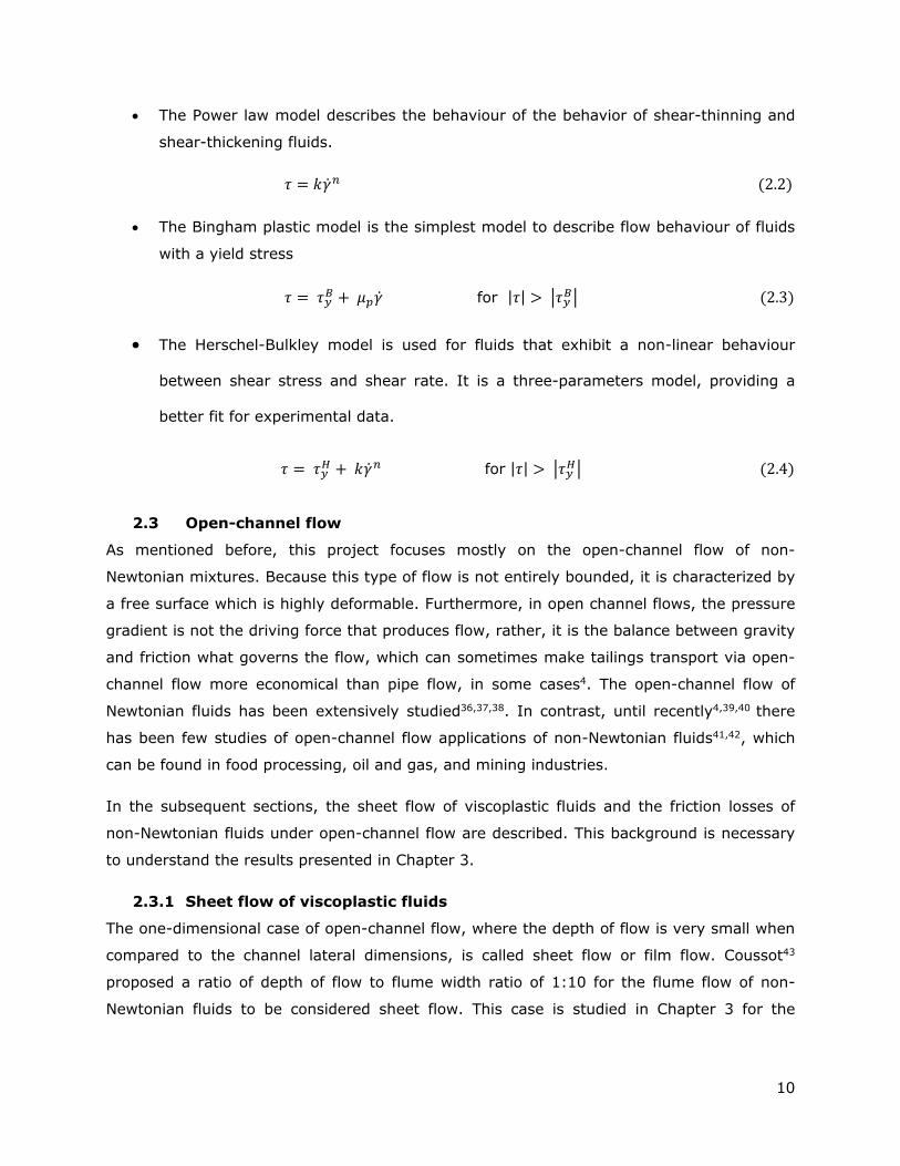
The Power law model describes the behaviour of the behavior of shear-thinning and

shear-thickening fluids.

𝜏 = 𝑘�̇�𝑛 (2.2)

The Bingham plastic model is the simplest model to describe flow behaviour of fluids

with a yield stress

𝜏 = 𝜏𝑦𝐵 + 𝜇𝑝�̇� for |𝜏| > |𝜏𝑦

𝐵| (2.3)

The Herschel-Bulkley model is used for fluids that exhibit a non-linear behaviour

between shear stress and shear rate. It is a three-parameters model, providing a

better fit for experimental data.

𝜏 = 𝜏𝑦𝐻 + 𝑘�̇�𝑛 for |𝜏| > |𝜏𝑦

𝐻| (2.4)

2.3 Open-channel flow

As mentioned before, this project focuses mostly on the open-channel flow of non-

Newtonian mixtures. Because this type of flow is not entirely bounded, it is characterized by

a free surface which is highly deformable. Furthermore, in open channel flows, the pressure

gradient is not the driving force that produces flow, rather, it is the balance between gravity

and friction what governs the flow, which can sometimes make tailings transport via open-

channel flow more economical than pipe flow, in some cases4. The open-channel flow of

Newtonian fluids has been extensively studied36,37,38. In contrast, until recently4,39,40 there

has been few studies of open-channel flow applications of non-Newtonian fluids41,42, which

can be found in food processing, oil and gas, and mining industries.

In the subsequent sections, the sheet flow of viscoplastic fluids and the friction losses of

non-Newtonian fluids under open-channel flow are described. This background is necessary

to understand the results presented in Chapter 3.

2.3.1 Sheet flow of viscoplastic fluids

The one-dimensional case of open-channel flow, where the depth of flow is very small when

compared to the channel lateral dimensions, is called sheet flow or film flow. Coussot43

proposed a ratio of depth of flow to flume width ratio of 1:10 for the flume flow of non-

Newtonian fluids to be considered sheet flow. This case is studied in Chapter 3 for the

11

validation of the CFD model to study the homogeneous, open-channel flow of non-

Newtonian mixtures.

In 1990, De Kee et al44. studied the steady, laminar, one dimensional, fully developed flow

of viscoplastic fluids along an inclined plane. They used the Herschel-Bulkley model, defined

in Equation (2.3), to describe the fluid behaviour, and proposed a laminar sheet model to

fully describe this type of flow; a schematic of the flow configuration can be seen in Figure

2.2.

Figure 2.2: Flow configuration for sheet flow reproduced from De Kee et al.44

By using the equations of continuity and motion, it was shown that:

𝜏𝑥𝑦 = 𝜌𝑔𝑥 sin 𝛼 (2.5)

At the wall, the maximum shear stress is determined by

𝜏𝑤 = 𝜌𝑔ℎ sin 𝛼 (2.6)

Figure 2.2 shows there is a plug-like region were the velocity will be constant, and hence,

the shear rate is zero whereas the shear stress is equal to the yield stress. In the plug,

described by, 0 ≤ x ≤ x0, the velocity is predicted using

𝑉𝑦< =

𝑛𝑘

(𝑛 + 1)𝜌𝑔 sin 𝛼(𝜏𝑤𝑘)(𝑛+1𝑛)

(1 −𝜏𝑦

𝜏𝑤)(𝑛+1𝑛)

(2.7)

α

Y

X

h Xo

𝑉𝑦<

𝑉𝑦>

Flow

12

Below the plug, where x0 < x ≤ h, the point velocity is given by

𝑉𝑦> =

𝑛𝑘

(𝑛 + 1)𝜌𝑔 sin 𝛼(𝜏𝑤𝑘)(𝑛+1𝑛)

(1 −𝜏𝑦


(

1 − (

𝜏𝑥𝑦𝜏𝑦

− 1

𝜏𝑤𝜏𝑦− 1

)

(𝑛+1𝑛)

)

(2.8)

The average velocity is given by

�̅� = 𝑛𝑘

(2𝑛 + 1)𝜌𝑔 sin𝛼(𝜏𝑤𝑘)(𝑛+1𝑛)

(1 −𝜏𝑦


(1 + (𝑛 + 1

𝑛)𝜏𝑦

𝜏𝑤) (2.9)

This model will be used in the simulation cases of Chapter 3. It was recently validated by

Haldenwang et al45, who performed experiments using Ultrasonic Velocity Profiling (UVP) to

characterize the behaviour of non-Newtonian fluids in a rectangular flume.

2.3.2 Friction losses on laminar, open-channel, flow of non-Newtonian fluids

Predicting the friction losses is an important component in designing and characterizing

open-channel flows. In this section, the different methods that have been proposed are

reviewed. These methods are most often based on a reworking of the Reynolds number.

Thus, a review of the Reynolds number definitions for non-Newtonian fluids is also provided.

Alderman and Haldenwang46 performed a review of the available models to predict the

open channel flow of non-Newtonian fluids in a rectangular channel using the experimental

data from Haldenwang and Slatter47. For laminar flow, the database consisted of

experimental data for CMC solutions, kaolin suspensions, and bentonite suspensions. An in-

line tube viscometer was used for rhelogical characterization. For each type of fluid, the

comparison was made by calculating the non-Newtonian Reynolds number as defined by

each author and the Fanning friction factor, for open-channel flow, defined as

𝑓 =2𝜏𝑤𝜌�̅�2

= 2𝑅ℎ𝑔 sin 𝜃

�̅�2 (2.10)

The calculated results were then compared against the following equation for laminar flow:

𝑓 =16

𝑅𝑒 (2.11)

Multiple definitions for the non-Newtonian Reynolds number have been proposed. Kozicki

and Tiu48 proposed a method for modelling the steady, fully developed laminar flow of any

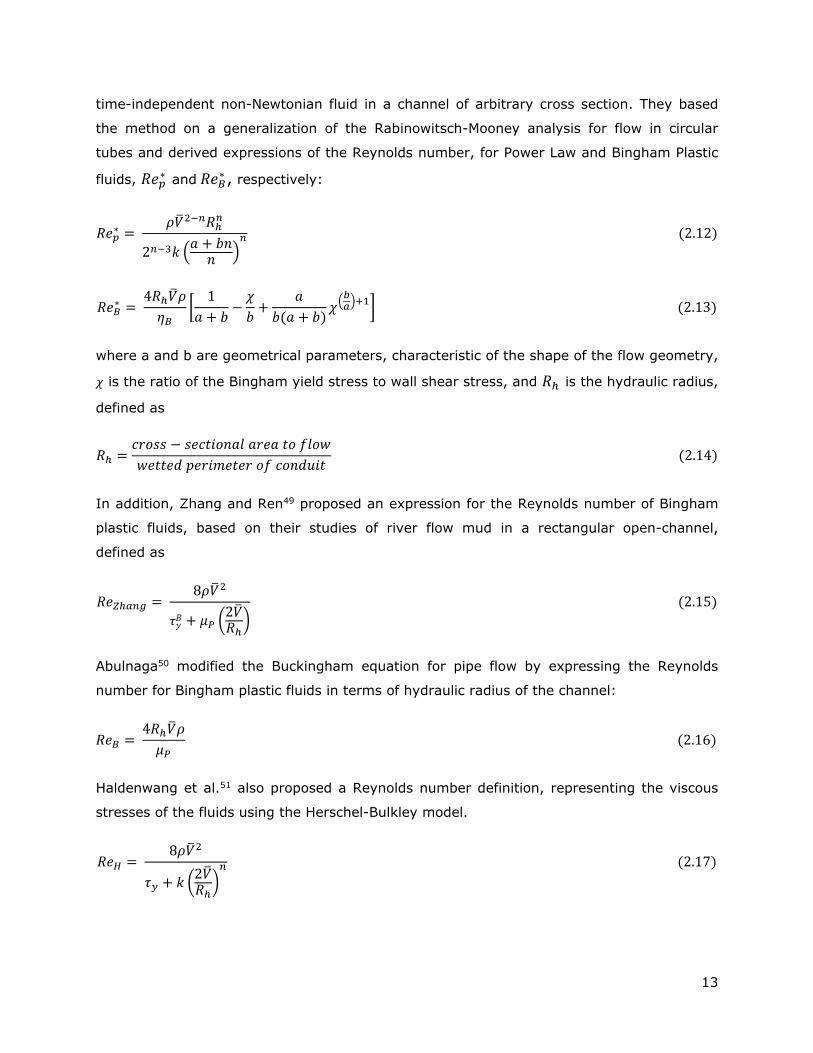
13

time-independent non-Newtonian fluid in a channel of arbitrary cross section. They based

the method on a generalization of the Rabinowitsch-Mooney analysis for flow in circular

tubes and derived expressions of the Reynolds number, for Power Law and Bingham Plastic

fluids, 𝑅𝑒𝑝∗ and 𝑅𝑒𝐵

∗ , respectively:

𝑅𝑒𝑝∗ =

𝜌�̅�2−𝑛𝑅ℎ𝑛

2𝑛−3𝑘 (𝑎 + 𝑏𝑛𝑛

)𝑛 (2.12)

𝑅𝑒𝐵∗ =

4𝑅ℎ�̅�𝜌

𝜂𝐵[1

𝑎 + 𝑏−𝜒

𝑏+

𝑎

𝑏(𝑎 + 𝑏)𝜒(𝑏𝑎)+1] (2.13)

where a and b are geometrical parameters, characteristic of the shape of the flow geometry,

𝜒 is the ratio of the Bingham yield stress to wall shear stress, and 𝑅ℎ is the hydraulic radius,

defined as

𝑅ℎ =𝑐𝑟𝑜𝑠𝑠 − 𝑠𝑒𝑐𝑡𝑖𝑜𝑛𝑎𝑙 𝑎𝑟𝑒𝑎 𝑡𝑜 𝑓𝑙𝑜𝑤

𝑤𝑒𝑡𝑡𝑒𝑑 𝑝𝑒𝑟𝑖𝑚𝑒𝑡𝑒𝑟 𝑜𝑓 𝑐𝑜𝑛𝑑𝑢𝑖𝑡 (2.14)

In addition, Zhang and Ren49 proposed an expression for the Reynolds number of Bingham

plastic fluids, based on their studies of river flow mud in a rectangular open-channel,

defined as

𝑅𝑒𝑍ℎ𝑎𝑛𝑔 = 8𝜌�̅�2

𝜏𝑦𝐵 + 𝜇𝑃 (

2�̅�𝑅ℎ)

(2.15)

Abulnaga50 modified the Buckingham equation for pipe flow by expressing the Reynolds

number for Bingham plastic fluids in terms of hydraulic radius of the channel:

𝑅𝑒𝐵 = 4𝑅ℎ�̅�𝜌

𝜇𝑃 (2.16)

Haldenwang et al.51 also proposed a Reynolds number definition, representing the viscous

stresses of the fluids using the Herschel-Bulkley model.

𝑅𝑒𝐻 = 8𝜌�̅�2

𝜏𝑦 + 𝑘 (2�̅�𝑅ℎ)𝑛 (2.17)

14

This definition can be used for Power Law, Bingham plastic, and Herschel-Bulkley fluids by

substituting the corresponding rheological parameters. During their experiments, they

evaluted carboxymethylcellulose (CMC) solutions, kaolin suspensions, and bentonite

suspensions.

As mentioned above, each Reynolds number definition was compared with the f = 16/Re

line. For Power Law fluids, the comparison was made between the definitions decribed by

Equations (2.12) and (2.17), and it was determined that both definitions predicted the

friction losses accuratelly, when compared with Equation (2.11). For Bingham platic fluids,

the comparison was made using the Reynolds number defined by Equations (2.13), (2.15),

(2.16), and (2.17). Only the definitions given by Equations (2.15) and (2.17) collapsed on

the f = 16/Re line accurately. For Herschel-Bulkley fluids, only the Reynolds number

defined by Equation 2.17 was available at the time and was found to predict the friction

losses accurately, when compared with Equation (2.11).

Burger et al.52 later confirmed that for non-Newtonian, laminar open-channel flows the

friction factor to Reynold number relationship depends on channel shape, similar to the case

of Newtonian, laminar, open-channel flow, where the laminar friction losses are defined by f

= K/Re, where K is a numerical constant dependent on channel shape36. Through their

experiments using flumes with different cross-sectional shapes, they determined values of

the constant K for rectangular, semi-circular, triangular, and trapezoidal flumes.

More recently, Burget et al.53 expanded that approach to turbulent flow regimes by using a

composite power law approach54, given by

𝑓 = 𝐹2 + (𝐹1 − 𝐹2)

(1 + (𝑅𝑒𝑡)𝑒

)𝑗 (2.18)

where 𝑒, 𝑡 and 𝑗 are fitting parameters; 𝐹1 and 𝐹2 are the power law relationships covering

the laminar and turbulent flows respectively:

𝐹1 = 𝑎𝑅𝑒𝑏 (2.19)

𝐹2 = 𝑐𝑅𝑒𝑑 (2.20)

In Equation (2.19) 𝑎 has same value of K, dependent of channel shape as mentioned above;

and 𝑏 has a numerical value of -1. In Equation (2.20) 𝑐 and 𝑑 are constants determined for

a modified Blasius Equation.

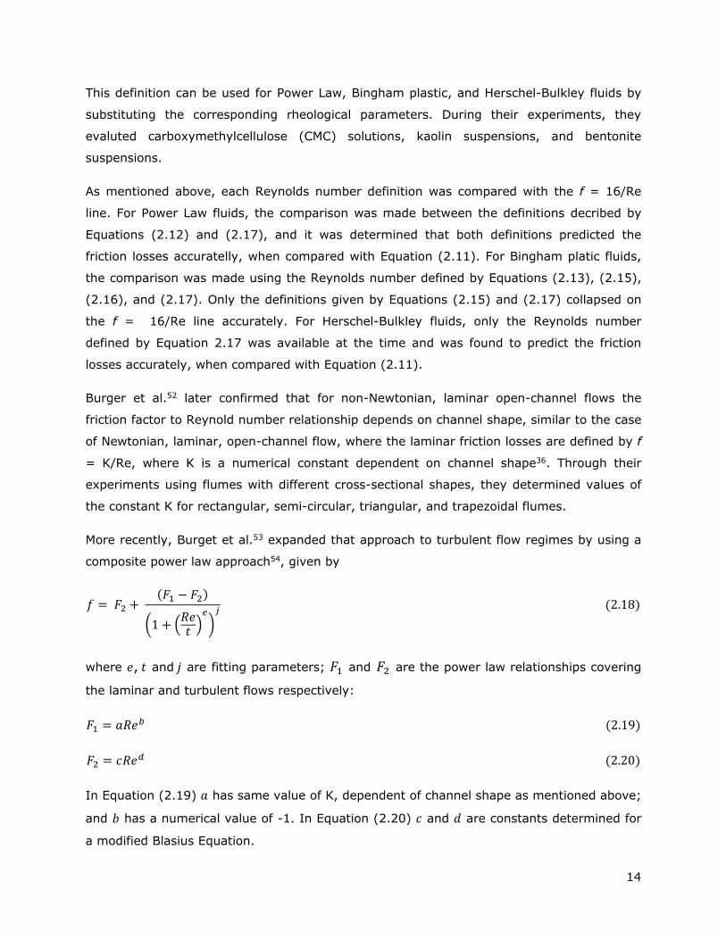
15

Based on the approach by Burger et al. 53, the Fanning friction factor for a Bingham plastic

fluid in a semi-circular channel can be written as

𝑓 = 0.048𝑅𝑒𝐻−0.2049 +

(16.2𝑅𝑒𝐻−1 − 0.048𝑅𝑒𝐻

−0.2049)

(1 + (𝑅𝑒𝐻1055

)230

)

0.015 (2.21)

where the Reynolds number is defined by Equation (2.17). Equation (2.21) can be

represented graphically as seen in Figure 2.3.

Figure 2.3: Moody diagram showing the relationship between the Fanning friction factor and

the Reynold number defined by Equation (2.21), with ReH defined by Equation (2.17)

2.4 Fluid-particle systems

Thickened tailings are complex clay-water-sand mixtures17. Ideally, we can divide these

mixtures into a non-Newtonian carrier fluid composed of the clay and water and a particle

phase composed of the sand particles. To model these mixtures, an understanding of how

fluids interact with solid particles within a suspension is critical.

This section starts by describing how a single particle behaves in a fluid. Specifically, the

settling under the effect of gravity of a particle through a Newtonian fluid is explained;

followed by a summary on recent advances and correlations to describe single-particle

settling through non-Newtonian fluids, as this is not fully understood yet. Understanding

how a single particle settles through non-Newtonian media acts as a basis to understand

16

settling of particles in a suspension. This background will be useful in understanding some

of the results presented in Chapter 4. Next, multi-particle systems are defined. The

hydrodynamics effects for dilute, semi-dilute, and concentrated suspensions are shown,

both for Newtonian and non-Newtonian fluids. Other phenomena such as particle migration

and sedimentation are shown, as these are prevalent in concentrated suspensions, such as

the ones that will be studied in Chapter 4 and 5

2.4.1 Single-particle systems

For a single spherical particle moving in a fluid. The Stokes’ law55 describes the total drag

force resisting slow, steady motion of a particle of diameter d, in a fluid of viscosity, µ:

𝐹𝐷 = 3𝜋𝑑𝜇𝑈 (2.22)

where U is the relative velocity between the particle and the fluid.

In addition, a single particle Reynolds number, 𝑅𝑒𝑝, and a drag coefficient, CD, can be

defined:

𝑅𝑒𝑝 = 𝑈𝜌𝑓𝑑

𝜇𝑓 (2.23)

𝐶𝐷 =

4𝐹𝐷𝜋𝑑2

12𝜌𝑓𝑈

2=

24

𝑅𝑒𝑝 (2.24)

Stokes’ law is only valid for 𝑅𝑒𝑝 < 0.3. At 𝑅𝑒𝑝 > 0.3 the fluid inertia begins to dominate the

motion because of the higher relative velocities. Table 2.1 shows the proposed correlations

for the calculation of the drag coefficient based on the particle’s Reynolds number.

Table 2.1: Drag coefficient correlations based on the particle’s Reynolds number

Region CD 𝑅𝑒𝑝 range

Stokes55 24

𝑅𝑒𝑝 𝑅𝑒𝑝 < 0.3

Intermediate56 24

𝑅𝑒𝑝(1 + 0.15𝑅𝑒𝑃

0.687) 0.3 < 𝑅𝑒𝑝< 500

Newton’s Law57 ~0.44 500 < 𝑅𝑒𝑝< 200000

17

i. Drag on a sphere in Newtonian fluids

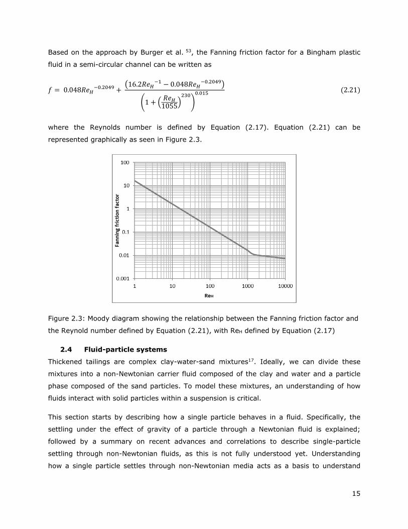
For a solid sphere falling under gravity through a Newtonian fluid, the force balance can be

given as57

Gravity Force (F𝐺) – Buoyancy Force (F𝐵) – Drag Force (F𝐷) = 0 (2.25)

A schematic representation is given by Figure 2.4.

Figure 2.4: Schematic representation of forces acting on a falling solid sphere

For a spherical particle, Equation (2.25) becomes,

𝜋𝑑3

6𝜌𝑠𝑔 −

𝜋𝑑3

6𝜌𝑓𝑔 −

1

2𝐶𝐷𝜌𝑓𝑉∞

2𝜋𝑑2

4= 0 (2.26)

Thus, the particle settling velocity is given by

𝑉∞ = √4𝑑𝑔(𝜌𝑠 − 𝜌𝑓)

3𝐶𝐷𝜌𝑓 (2.27)

where CD is the drag coefficient, and can be related to the particle’s Reynolds number, 𝑅𝑒𝑝,

as shown in Table 2.1

ii. Drag on a sphere in non-Newtonian fluids

In power law fluids, the drag coefficient can be expressed in terms of the Reynolds number

and the power law index. For the creeping flow region (Re << 1), the result can be

expressed as a deviation factor X(n), from Stokes’ law:

FG

FB

FD

18

𝐶𝐷 = 24

𝑅𝑒𝑃𝐿𝑋(𝑛) (2.28)

where X(n)58 and RePL59 are defined by

𝑋(𝑛) = 6(𝑛−1)/2 (3

𝑛2 + 𝑛 + 1)𝑛+1

(2.29)

𝑅𝑒𝑃𝐿 = 𝜌𝑉2−𝑛𝑑𝑛

𝑘 (2.30)

For 𝑅𝑒𝑃𝐿 ≤ 500 the values of drag coefficient are represented by the following equation60:

𝐶𝐷 = 24

𝑅𝑒𝑃𝐿(1 + 0.148𝑅𝑒𝑃𝐿

2.35𝑛

2.42𝑛+0.918) (2.31)

In viscoplastic fluids, a parameter is introduced which describes, for a spherical particle, the

static equilibrium between gravity and the yield stress of a fluid61:

𝑌𝐺 = 𝜏𝑦

𝑔𝑑(𝜌𝑠 − 𝜌𝑓) (2.32)

Although this parameter theoretically is intended to provide insight on the balance of forces

around a sphere, several studies have reported different YG values. For example, Beris et

al.62 reported YG ~ 1/21 from their simulation results by solving the equations of motion,

which was later confirmed through experiments conducted by Tabuteau et al.63. Other

researchers have reported YG ~ 0.2 based on the assumption that the buoyant weight of a

sphere is supported by the vertical component of the force due to the yield stress acting

over the sphere surface64,65,66. The discrepancies seem to be related to the yield stress

measurement methods and the underlying differences surrounding the way the yield stress

has been measured61.

Once the sphere starts to move the flow field will have a characteristic shape, refered to as

a sheared envelope. As the shear stress decreases to a value below the fluid yield stress,

the fluid will no longer flow and will behave as an elastic solid. The shape and size of the

envelope is dependent on the carrier fluid yield stress, the size and density of the sphere

and the relative velocity between the sphere and the fluid61. Figure 2.5 shows examples of

the sheared envelope as depicted by various investigators62,67,68.

19

Figure 2.5: Shape of the sheared envelope surroinding a sphere in creeping motion through

viscoplastic fluids: (a) Ansley and Smith67, (b) Yoshioka et al68., (c) Beris et al.62 from61.

For most applications of a settling sphere through a yield stress fluid, correlations are used

to determine the drag coefficient (and hence, the terminal settling velocity). An extensive

review of the available correlations can be found elsewhere61. Thus, only methods relevant

to the modelling of Chapter 4 will be explained here.

Atapattu et al.69 extended the analysis of Ansley and Smith67, and developed a method for

predicting the drag coefficient from their experimental data using

𝐶𝐷 = 24

𝑄∗ (2.33)

where,

𝑄∗ = 𝑅𝑒𝑃𝐿

1 +7𝜋24𝐵𝑖𝐻𝐵

(2.34)

𝐵𝑖𝐻𝐵 = 𝜏𝑦𝐻

𝑘 (𝑉∞𝑑)𝑛 (2.35)

20

While this correlation collapses the data to the Newtonian standard drag curve, it was

limited to experiments using Herschel-Bulkley fluids where 0.43 ≤ n ≤ 0.84, and 10-8 ≤ Q*

≤ 0.3. Consequently, for systems with Q* > 0.3 the error in prediction increases

dramatically35.

Wilson et al.70 proposed a direct method to calculate the terminal settling velocity of a

sphere in a viscoplastic fluid by implementing the pipe flow analysis of Prandtl71 and

Colebrook72. Since the shear stress distribution is not uniform around a particle, the

characteristic shear stress was defined as the mean surficial stress (𝜏̅) of a falling particle,

relating the immersed weight of the particle to its surface area:

𝜏̅ = 𝑑𝑔(𝜌𝑠 − 𝜌𝑓)

6 (2.36)

The particle shear velocity is defined as

𝑉∗ = √�̅�

𝜌𝑓= √

𝑑𝑔(𝜌𝑠 − 𝜌𝑓)

6𝜌𝑓 (2.37)

In addition, the shear Reynolds number is defined by

𝑅𝑒∗ = 𝑑𝜌𝑓𝑉

∗

𝜇 (2.38)

Wilson et al.70 represented the Newtonian drag curve in a V∞/V* vs Re* plot. An apparent

viscosity is calculated from the fluid and particle properties and then the terminal settling

velocity is calculated for an equivalent case in a Newtonian fluid using the apparent

viscosity. A reference point of 0.3𝜏̅ in the fluid rheogram was proposed to determine the

proper apparent viscosity from the equivalent Newtonian viscosity. The results from this

approach can be seen in Figure 2.6.

21

Figure 2.6: Relative fall velocity versus Reynolds number70 with 𝜏𝑟𝑒𝑓 = 0.3𝜏̅

While this method works very well for Re* > 100, its predictions seem to deviate noticeably

when Re* <100. In addition, the method is limited for systems where 0.3𝜏̅ > 𝜏𝑦, since

there are no points from the reogram when the reference point is below the yield stress.

In an effort to improve this method, Shokrollahzadeh35 performed high-quality

measurements of terminal settling velocities of single spheres in viscoplastic fluids and

developed a correlation using the analogy of the Wilson-Thomas model for the turbulent

pipe flow of Newtonian fluids73 defined by:

𝜇𝑎𝑝𝑝 = {𝜇𝑒𝑞(4.586𝛼

12.878𝜉1.612), 𝑓𝑜𝑟 𝛼 < 1.3

𝜇𝑒𝑞(5.139𝜉1.55𝑒(𝛼

3.995) + 𝜉2.747 + 0.731), 𝑓𝑜𝑟 𝛼 ≥ 1.3 (2.39)

where 𝛼, for a Bingham Plastic fluid, is given by

𝛼𝐵 = 1 + 𝜏𝑦𝐵

𝜏̅ (2.40)

𝜉 = 𝜏𝑦

𝜏̅ (2.41)

The results from this correlation can be seen in Figure 2.7. Later in Chapter 4, it will be

shown that this correlation can be used in the modelling of a single-particle settling in a

non-Newtonian fluid with better accuracy than other correlations.

22

Figure 2.7: Equation (2.39) prediction using experimental data from Valentik and

Whitmore74, Ansley and Smith67, Wilson et al.70, Tran et al.75, and Shokrollahzadeh35.

2.4.2 Multi-particle systems

In this section, multi-particle systems are described. Specifically, the phenomena resulting

from interactions between particles and carrier fluids are considered. These are of

importance for the modelling results showed in Chapters 4 and 5.

First, the hydrodynamic effects in Newtonian suspensions are shown, followed by recent

studies of non-Newtonian suspensions. Next, particle migration is introduced which is of

concern primarily for concentrated suspensions. Finally, sedimentation of particles both in

Newtonian and non-Newtonian suspensions is shown.

i. Hydrodynamic effects

When particles are added to a Newtonian fluid, its resistance to flow increases. This

behaviour was seen experimentally by Rutgers76. The relative viscosity, 𝑟, is defined by

𝑟=

𝑠

𝑐

(2.42)

23

where 𝑠 is the viscosity of the suspension, and

𝑐 is the viscosity of the carrier fluid. For

monodisperse spheres, the relative viscosity is an increasing function of the particle volume

fraction. From a physical point of view, solid particles can contribute to the viscosity in two

ways: first, the distortion of the flow lines because of the volume occupied by a particle in

the fluid and second, the surface roughness of the particle24.

For dilute systems, where the interactions between the particles can be neglected, Einstein

proposed the following expression for the relative viscosity77

𝑟= 1 + 2.5𝜙 (2.43)

where 𝜙 is the particle volume fraction.

In semi-dilute systems, where 𝜙 ~ 0.1, the distance between the particles cannot be

neglected, since the presence of a second particle alters the flow field significantly, which

changes the viscosity. The interaction between pairs of particles will be proportional to the

square of the volume fraction24:

𝑟= 1 + 2.5𝜙 + 𝐶2𝜙

2 +⋯ (2.44)

The quadratic coefficient, 𝐶2, can have different values depending on the particle shape,

particle size distribution, and particle surface roughness24.

In concentrated systems, the average distance between particles becomes sufficiently small

for lubrication hydrodynamic interactions to dominate the stresses24. Under shear flow,

experimental studies of the microstructure has shown the flow field to be anisotropic78. In

contrast to semi-dilute and dilute systems, the maximum packing concentration, 𝜙𝑚𝑎𝑥,

must be taken into account in any calculation involving concentrated suspensions, as flow

will cease once this limit is met (i.e. when particles are closely packed). The value of 𝜙𝑚𝑎𝑥

depends on particle shape and particle size distribution; for a spherical particle24 𝜙𝑚𝑎𝑥 ~

0.6.

Exact predictions of the suspension viscosity do not exist; thus, a number of semi-empirical

relations have been proposed, most of which will be used in the modelling of multi-particle

systems. For example, Krieger and Dougherty proposed25,26

𝑟= (1 −

𝜙

𝜙𝑚𝑎𝑥)−[]𝜙𝑚𝑎𝑥

(2.45)

24

where [] is equal to 2.5 for spherical particles. Thomas79 proposed the following expression

based on experimental data:

𝑟= 1 + 2.5𝜙 + 10.05𝜙2 + 0.00273𝑒(16.6𝜙) (2.46)

Morris and Boulay27 proposed the following expression for monodispersed spheres,

𝑟= 1 + 2.5𝜙 (1 −

𝜙

𝜙𝑚𝑎𝑥)−1

+ 𝐾𝑠 (𝜙

𝜙𝑚𝑎𝑥)2

(1 −𝜙


(2.47)

where Ks is the contact contribution and has a value of 0.1.

In addittion, Gillies et al.32 proposed

𝑟= 1 + 2.5𝜙 + 10𝜙2 + 0.0019𝑒(20𝜙) (2.48)

based on their experiments of sand particles suspended in a Newtonian fluid.

The effect of particle concentration on the apparent viscosity for non-Newtonian fluids has

also been studied. Chakrabandhu and Singh80 determined, from their experiments using

green peas suspended in a CMC solution, expressions for the relative viscosity, and

consistency coefficient for their conditions: specifically, temperatures from 85 to 135 °C,

and shear rates from 33 to 247 s-1 .

𝑟= 1 + 2.5𝜙 + 10.05𝜙2 + 20.84𝜙3 (2.49)

𝑘𝑟 =𝑘(𝜙)

𝑘 (0)= (1 + 2.5𝜙)𝑛𝑟

−2 (2.50)

where Kr and nr are the relative consistency coefficient and flow index, respectively.

More recently, Mahaut et al81., Chateau et al82., and Ovarlez et al83., have studied the

effects of coarse, monodispersed, spherical particle concentration on the suspension yield

stress and consistency, and have represented the effect as follows:

𝜏𝑦𝑟 = 𝜏𝑦(𝜙)

𝜏𝑦(0)= √(1 − 𝜙) (1 −

𝜙

𝜙𝑚𝑎𝑥)−2.5𝜙𝑚𝑎𝑥

(2.51)

𝑘𝑟 = 𝑘(𝜙)

𝑘 (0)= √((1 −

𝜙

𝜙𝑚𝑎𝑥)−2.5(𝑛+1)𝜙𝑚𝑎𝑥

) (1 − 𝜙)1−𝑛 (2.52)

25

Equations 2.51 and 2.52 were developed for 250 µm polystyrene particles suspended in a

concentrated emulsion, which was characterized as a Herschel-Bulkley fluid. The flow

behaviour of the suspension was evaluated in Couette geometry at shear rates from 0.01 to

80 s-1, with bulk particle volume fractions from 0.1 to 0.5. The equations above provided

good agreement when compared with their experiments; however, Ovarlez et al.83 made no

comments on their applicability to Bingham plastic fluids or in tube geometries. Despite this,

an attempt to use their equations in the modelling conditions of Chapter 5 will be made.

ii. Particle migration

Non-hydrodynamic effects such as interparticle forces can break the particle trajectories

causing diffusion and migration24. Furthermore, in concentrated suspensions, the

interactions between the particles result in chaotic motion84, which generates displacements

in various directions. Flow-induced self-diffusion, described as the random motion of a

particle in a flow field, was first reported by Eckstein et al85.

Shear-induced migration occurs when there are gradients in shear rate. This was shown by

Leighton and Acrivos28, where neutrally buoyant particles migrated to toward the cup (outer

cylinder) of a coaxial cylinder device during their experiments.

In the work of Phillips et al.30, the migration has been modelled using a local diffusion with a

diffusion flux model, and the significant driving forces for particle transport have been

reduced into two partial fluxes. The first flux is due to spatially varying interaction

frequency; i.e, particles moving from regions of high shear rate to regions of low shear rate:

𝑁𝑐 = −𝐾𝑐𝜙𝑎2∇(�̇�𝜙) (2.53)

The second flux is due to spatially varying viscosity:

𝑁 = −𝐾𝑎2�̇�𝜙2

(𝜙)∇((𝜙)) (2.54)

where 𝐾𝑐 and 𝐾 are proportionality constants and have values of 0.43 and 0.65,

respectively30.

Another approach to model migration is to relate the normal stresses or a “normal viscosity”

caused by the presence of particles as follows27:

𝑛= 𝐾𝑛 (

𝜙

𝜙𝑚𝑎𝑥)2

(1 −𝜙


(2.55)

26

where 𝐾𝑛 is the normal contact contribution and has a value of 0.75.

Shear-induced migration in non-Newtonian fluids has not been studied extensively. Rao et

al86 extended the Phillips model characterized by equations (2.53) and (2.54), to shear-

thinning fluids, which captured many of the trends from their experiments but failed to

agree quantitavely.

Ovarlez et al83. were able to predict theoretically shear-induced migration by relating it to

the normal stress differences in a concentric-cylinder Couette flow for yield stress fluids.

Moreover, the expression they derived is the same as for particles suspended in a

Newtonian fluid27, provided the carrier fluids have similar microstructure and the yield stress

suspension is sheared in the whole gap of the Couette geometry.

iii. Sedimentation

In concentrated suspensions, the settling of the particles is hindered when compared to the

single-particle settling process described in Section 2.4.1. The sedimentation can be

described by the empiricial expression by Richardson and Zaki31.

𝑉∞,𝑠𝑉∞

= (1 − 𝜙)𝑛 (2.56)

where 𝑉∞,𝑠 is the hindered settling rate of the particles, and 𝑛 is an empirical constant,

which is known to be influenced experimentally by wall effects87, particle size distribution88,

and flow regime.

For shear flow, Spelay17 extended the Phillips model, described by Equations (2.53) and

(2.54), to include a sedimentation flux as follows

𝑁𝑠 = 𝐾𝑠𝑎2𝜙𝑓(𝜙)�⃗� (2.57)

where

𝐾𝑠 = 2(𝜌𝑠 − 𝜌𝑓)

9 (2.58)

𝑓(𝜙) = (1 − 𝜙)

𝑠

(2.59)

In addition, Ovarlez et al.89 studied the shear-induced sedimentation of monodispersed,

glass particles in two yield stress fluids: a concentrated emulsion and Carbopol solution;

27

using a Coeutte cell. They determined that shear induces sedimentation in all the studied

systems, even in those stable at rest as per 𝑌𝐺 values (defined by Equation 2.32), and it can

be modelled by considering that the insterstitial fluid behaves like a viscous fluid in the

direction orthogonal to the shear. An increase in particle concentration was found to play

two roles: hinders settling and, at the same time, it decreases the viscous resistance of the

interstitial fluid because of shear concentration between the particles. At the plastic regime

(i.e. BiHB-1 << 1, as defined by Equation 2.35), they proposed a method to predict particle

sedimentation, defined by:

𝑉(𝜙) = 𝛼∆𝜌𝑔𝑑2

[�̇�𝑙̅ (𝜙)]

𝑓𝑁𝑒𝑤𝑡𝑜𝑛𝑖𝑎𝑛(𝜙) (2.60)

While Equation (2.60) agrees well with their experimental observations, Ovarlez et al.89

pointed out that it would be difficult to compare their experimental results with analytical or

numerical studies, because of the poor reproducibility of the concentrated emulsion, and

shear rate heterogeneities within the gap of the Couette cell. However, a qualitative

analysis, to summarize their results, can be made from Equation (2.60): the sedimentation

velocity increases with shear rate and for a given particle diameter and shear rate, the

sedimentation velocity is a decreasing function of the fluid yield stress. For a viscoplastic

fluid with given rheological properties, the sedimentation velocity is an increasing function

of particle diameter. These statements will be useful in testing the model in Chapter 5.

2.5 Numerical modelling

This section provides relevant background for the modelling of viscoplastic fluids, where two

main approaches are described, one of which is used during this project. In regard to

modelling suspensions, the main challenges are described, along with a review of relevant

numerical studies.

2.5.1 Numerical modelling of viscoplastic fluids

The challenge in modelling yield stress fluid flow is to properly represent the plug-like

region, where the shear stress is below the yield stress, and to track the surfaces that

separate the plug zones from the sheared zones23. Two approaches have been developed to

overcome these challenges. One approach relies on augmented Lagrangian methods to

solve the Navier-Stokes equations via an optimization algorithm90. The other method

regularizes the constitutive law for viscoplastic fluids. For an ideal viscoplastic fluid, the

apparent viscosity becomes infinite at the plug region; the method replaces this with a very

28

viscous fluid. Regularization methods are often the preferred approach because of their

simplicity of implementation in commercial CFD packages through user-defined functions91.

2.5.2 Numerical modelling of coarse particle suspensions

Modelling concentrated suspensions poses numerous challenges as many-body

hydrodynamic interactions must be calculated, while also resolving the spatial distribution of

the particles in the fluid. Since there is no exact method to predict how the viscosity varies

with the presence of particles24, various methods have been applied for approximation of

the many-body hydrodynamic interactions. Examples include Stokesian92 dynamics, the

Lattice Boltzmann93 method, and dissipative particle94 dynamics. However, these methods

become very limited when the concentration tends towards the maximum packing

concentration, since the particles all nearly touch, the time-step required to accurately

resolve motion tends to zero95. This is usually resolved by adding fictitious surface forces or

limitations on the forces acting between the particles24.

Spelay17 developed a code to model the laminar open-channel flow of negatively-buoyant

particles suspended in a viscoplastic fluid, by using the model defined by Equations (2.53),

(2.54), and (2.57), and successfully compared it with his experimental data. However, the

model is limited to laminar one-dimensional flow of suspensions, and it is not able to predict

the sliding bed moving en-bloc.

Most commercial CFD packages rely on the Granular Kinetic Theory (GKT) to account for the

behaviour of concentrated coarse particle suspensions. Ekambara et al96 studied the

horizontal slurry transport under turbulent regime using ANSYS-CFX as the CFD solver, and

the GKT model. Their model is able to predict coarse particle concentration profiles in

turbulent pipe flow, which they found to be primarly dependent upon the in-situ solids

volume fraction. In addition, the model was validated sucessfully against available

experimental data.

Eesa and Barigou97 studied the horizontal and vertical flow of coarse nearly-neutrally

buoyant particles in power law carrier fluids using ANSYS-CFX and the GKT model. Their

model was able to predict the particle phase velocity profile and pressure drop, which were

compared against experimental data and available correlations.

Treinen and Jacobs33 used Ansys Fluent and the GKT model to study particle settling and

shear migration in viscoplastics fluids. Three modelling scenarios were considered: quasi-

static settling, shear particle migration, and shear settling of particles. Their CFD model

predicted quasi-static settling in Newtonian fluids but it was not able to predict the

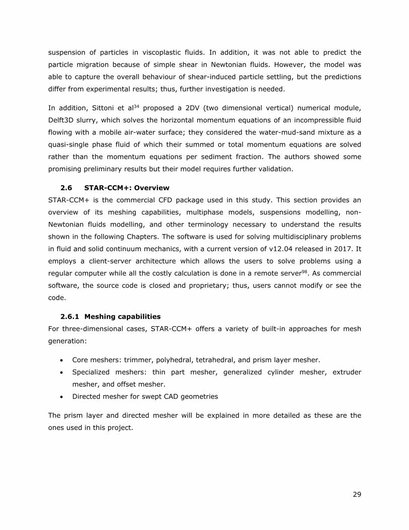
29

suspension of particles in viscoplastic fluids. In addition, it was not able to predict the

particle migration because of simple shear in Newtonian fluids. However, the model was

able to capture the overall behaviour of shear-induced particle settling, but the predictions

differ from experimental results; thus, further investigation is needed.

In addition, Sittoni et al34 proposed a 2DV (two dimensional vertical) numerical module,

Delft3D slurry, which solves the horizontal momentum equations of an incompressible fluid

flowing with a mobile air-water surface; they considered the water-mud-sand mixture as a

quasi-single phase fluid of which their summed or total momentum equations are solved

rather than the momentum equations per sediment fraction. The authors showed some

promising preliminary results but their model requires further validation.

2.6 STAR-CCM+: Overview

STAR-CCM+ is the commercial CFD package used in this study. This section provides an

overview of its meshing capabilities, multiphase models, suspensions modelling, non-

Newtonian fluids modelling, and other terminology necessary to understand the results

shown in the following Chapters. The software is used for solving multidisciplinary problems

in fluid and solid continuum mechanics, with a current version of v12.04 released in 2017. It

employs a client-server architecture which allows the users to solve problems using a

regular computer while all the costly calculation is done in a remote server98. As commercial

software, the source code is closed and proprietary; thus, users cannot modify or see the

code.

2.6.1 Meshing capabilities

For three-dimensional cases, STAR-CCM+ offers a variety of built-in approaches for mesh

generation:

Core meshers: trimmer, polyhedral, tetrahedral, and prism layer mesher.

Specialized meshers: thin part mesher, generalized cylinder mesher, extruder

mesher, and offset mesher.

Directed mesher for swept CAD geometries

The prism layer and directed mesher will be explained in more detailed as these are the

ones used in this project.

30

i. Prism layer mesher

The prism layer mesher is used in conjunction with other meshing techniques to generate

cells that are orthogonal to the wall surfaces or boundaries, which allows the CFD solver to

resolve near-wall flow more accurately, as well as flow features such as separation which

can affect drag or pressure drop results. The layers are characterized by their thickness,

number of cell layers, and size distribution; these features can be modified accordingly to

the needs of the user98, as shown in Figure 2.8.

(a)

(b)

Figure 2.8: Prism layer mesher example, with (a) Progressive layer stretching and (b)

Constant stretching

ii. Directed Meshing

The directed meshing technique is used to create a surface mesh and sweep it in a given

direction of the CAD geometry through its volume. This allows for stretching and control

over the mesh resolution in the direction where large gradients of the flow variables are not

expected98.

The surfaces of the geometry can be divided in the following categories for direct meshing:

Source surface, where the surface mesh is initially generated

Target surface, where the meshing ends

Guide surface, alongside which the surface mesh is swept from the source surface to

the target surface

A graphical representation of the categories can be seen in Figure 2.9.

31

Figure 2.9: (a) Source, (b) target, and (c) guide surfaces for directed meshing

The source surface mesh is related with a volume mesh distribution which is used to

generate the final volume mesh, which can be seen in Figure 2.10.

Figure 2.10: Directed mesh example

(a)

(b)

(c)

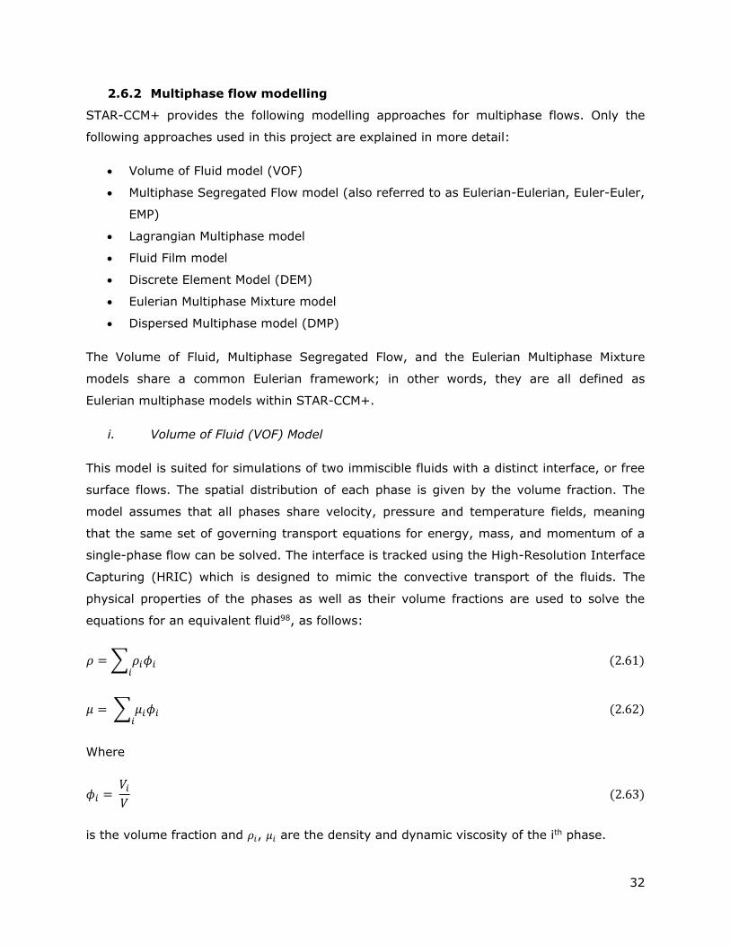
32

2.6.2 Multiphase flow modelling

STAR-CCM+ provides the following modelling approaches for multiphase flows. Only the

following approaches used in this project are explained in more detail:

Volume of Fluid model (VOF)

Multiphase Segregated Flow model (also referred to as Eulerian-Eulerian, Euler-Euler,

EMP)

Lagrangian Multiphase model

Fluid Film model

Discrete Element Model (DEM)

Eulerian Multiphase Mixture model

Dispersed Multiphase model (DMP)

The Volume of Fluid, Multiphase Segregated Flow, and the Eulerian Multiphase Mixture

models share a common Eulerian framework; in other words, they are all defined as

Eulerian multiphase models within STAR-CCM+.

i. Volume of Fluid (VOF) Model

This model is suited for simulations of two immiscible fluids with a distinct interface, or free

surface flows. The spatial distribution of each phase is given by the volume fraction. The

model assumes that all phases share velocity, pressure and temperature fields, meaning

that the same set of governing transport equations for energy, mass, and momentum of a

single-phase flow can be solved. The interface is tracked using the High-Resolution Interface

Capturing (HRIC) which is designed to mimic the convective transport of the fluids. The

physical properties of the phases as well as their volume fractions are used to solve the

equations for an equivalent fluid98, as follows:

𝜌 =∑ 𝜌𝑖𝜙𝑖 𝑖

(2.61)

𝜇 = ∑ 𝜇𝑖𝜙𝑖 𝑖

(2.62)

Where

𝜙𝑖 = 𝑉𝑖𝑉 (2.63)

is the volume fraction and 𝜌𝑖, 𝜇𝑖 are the density and dynamic viscosity of the ith phase.

33

Thus, the conservation equation for the transport of volume fraction 𝜙𝑖 is:

𝑑

𝑑𝑡∫𝜙𝑖𝑑𝑉

𝑉

+∫𝜙𝑖(𝐯 − 𝐯𝑔) ∙ 𝑑𝐚 = ∫(𝑆𝜙𝑖 −𝜙𝑖𝜌𝑖

𝐷𝜌𝑖𝐷𝑡) 𝑑𝑉

𝑉𝑆

(2.64)

ii. Multiphase Segregated Flow model

This model is based on an Eulerian-Eulerian formulation where the conservation equations

are solved for each distinct phase; the pressure equation is shared by all phases, while the

volume fraction gives the share of the flow domain each phase occupies. The model uses a

SIMPLE-type (Semi-Implicit Method for Pressure Linked Equations) approach as a solution

algorithm, which has separate pressure and velocity solvers98.

The conservation of momentum is given by

𝜕

𝜕𝑡∫𝜙𝑖𝜌𝑖𝜒𝑽�̇�𝑑𝑉

𝑉

+∮ 𝜙𝑖𝜌𝑖𝜒𝑽�̇� ⊗ (𝑽�̇� − 𝑽𝒈) ⋅ 𝑑𝒂𝐴

= − ∫𝜙𝑖𝜒∇𝑝𝑑𝑉

𝑉

+ ∫𝜙𝑖𝜌𝑖𝜒𝒈𝑑𝑉

𝑉

+∮ [𝜙𝑖(𝜏𝑖 + 𝜏𝑖𝑡)]𝜒 ⋅ 𝑑𝒂

𝐴

+ ∫𝐌𝑖𝜒𝑑𝑉

𝑉

+ ∫

𝑉

(𝐅𝑖𝑛𝑡)𝑖𝜒𝑑𝑉 + ∫ 𝑠𝑖𝑉 𝑑𝑉

𝜈

+ ∫𝛴𝑗≠𝑖(𝑚𝑖𝑗𝑽𝒋̇ −𝑚𝑗𝑖𝑽�̇�)𝜒 𝑑𝑉

𝑉

(2.65)

And, the conservation of mass is given by

𝜕

𝜕𝑡∫𝜙𝑖𝜌𝑖𝜒𝑑𝑉

𝑉

+ ∮ 𝜙𝑖𝜌𝑖𝜒(𝑽�̇� − 𝑽𝒈) ⋅ 𝑑𝒂𝐴

= ∫𝛴𝑗≠𝑖(𝑚𝑖𝑗 −𝑚𝑗𝑖)𝜒 𝑑𝑉

𝑉

+∫𝑠𝑖𝛼 𝑑𝑉

𝜈

(2.66)

The topology and physics of the interface between two phases are defined by phase

interactions in STAR-CCM+, each one identifies which phases interact, the interface

topology, models for the interface length, and interphase transfers98.

For multiphase segregated flows, these phase interactions are available:

Granular Particle Pair, used to define the interaction between two particle phases.

Continuous-Dispersed, used to define a phase that is dispersed in a continuous

phase.

Large Scale Interface (LSI), used for stratified two-phase flow with a dispersed two-

phase flow.

34

The Continuous-Dispersed phase interactions are of interest for this investigation. When

selecting the Continuous-Dispersed phase interaction the following models are automatically

selected:

Drag force, modelled as a linear multiplier of the relative velocity between two

phases

Interaction Length Scale, defined as the mean particle size, is used to calculate

Reynolds number and interaction area density

Interaction Area Density, specifies the interfacial area available for drag, and mass

transfers between phases

Also, when the continuous phase is a liquid and the dispersed phase is a bubble or a solid

particle, the suspension rheology model can be activated as additional modelling for the

phase interactions. As pointed out earlier, the presence of particles suspended in a liquid

has a strong effect on the mixture viscosity. STAR-CCM+ provides the following built-in

models for the relative viscosity: Krieger-Dougherty Model, defined by Equation (2.45); and

the Morris and Boulay model, defined by Equation (2.47). The normal viscosity can be

modelled using Equation (2.55). Also, the following interface transfer models available:

Lift force, used to model the perpendicular lift force that a particle can experience in

a non-uniform flow field

Wall lubrication force, used to model the force that a rising bubble experiences that

prevents it from touching the wall

Turbulent dispersion force, used to model the interaction between the dispersed

phase and the turbulent eddies

Virtual mass force, used to model an additional resistance that a particle experiences

accelerating through a fluid

iii. Lagrangian multiphase model

The Lagrangian model is designed to track the path of particles dispersed in a continuous

phase. In a Lagrangian frame, the conservation equations are solved for each individual

particle, which allows the user to calculate the trajectory of each particle. On the other

hand, the governing equations for the continuous phase are solved in an Eulerian frame

taking into account the dispersed phase98.

The interaction between the dispersed phase and the continuous phase can be modelled as

one-way coupling or two-way-coupling. In one-way coupling, the continuous phase

35

influences the dispersed phase but not the other way around. In two-way coupling the

continuous phase and the dispersed phase influence each other98.

The momentum conservation equation for a particle in a Lagrangian framework is given by

𝑚𝑝

𝑑𝒗𝑝

𝑑𝑡= 𝑭𝑠 + 𝑭𝑏 (2.67)

where 𝑭𝑠 denotes the surface forces action on the particle and 𝑭𝑏 represents the body

forces. Particles are introduced to the flow domain through discrete injectors, which define

the size and velocity of the particles.

2.6.3 Non-Newtonian flow modelling

Non-Newtonian fluids can be modelled in STAR-CCM+ using built-in models or user-defined

functions. Specifically, the non-Newtonian Generalized Power Law model uses the

regularization method, described in Section 2.5.1: at the plug region, the viscosity of the

mixture is modelled as a very high viscosity fluid; at the sheared region, the viscosity of the

mixture varies with shear rate. The formulation of the model is described by

𝜇(�̇�) =

{

𝑎𝑇 ∗ 𝜇0 , �̇� <

𝜏𝑦

𝜇0

𝑎𝑇 ∗𝜏𝑦 + 𝑘 [𝑎𝑇 (�̇� −

𝜏𝑦𝜇0)]𝑛

𝑎𝑇�̇� , �̇� >

𝜏𝑦

𝜇0

(2.68)

where 𝑎𝑇 is a temperature factor and 𝜇0 is the yielding viscosity, which is the value of

dynamic viscosity the solver uses at the plug region.

2.6.4 Solution Analysis

Simulation data can be accessed through field functions in STAR-CCM+, while the simulation

is running and when it is completed. The following strategies can be used to analyze the

data:

Reports, which can be created for specific quantities and can be monitored while the

simulation is running.

Scenes, which allow for dynamic viewing of a running simulation or converged

solution

Plots, which can be created using sets of data from the solution

Regardless of the chosen strategy, the parts that represent the actual size and shape of the

physical space from which the solution is extracted must be selected:

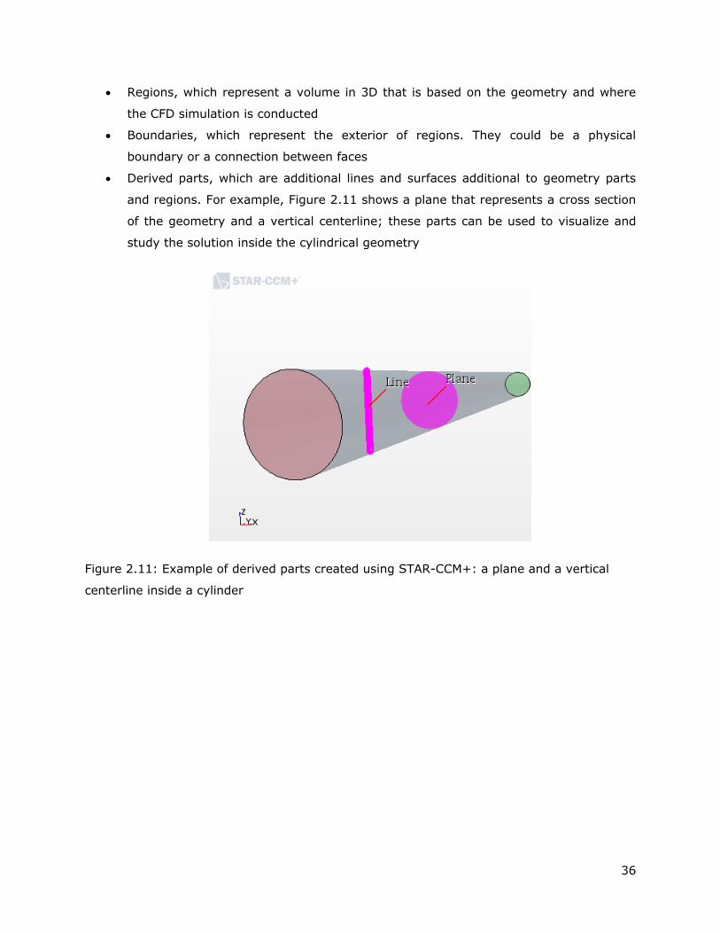
36

Regions, which represent a volume in 3D that is based on the geometry and where

the CFD simulation is conducted

Boundaries, which represent the exterior of regions. They could be a physical

boundary or a connection between faces

Derived parts, which are additional lines and surfaces additional to geometry parts

and regions. For example, Figure 2.11 shows a plane that represents a cross section

of the geometry and a vertical centerline; these parts can be used to visualize and

study the solution inside the cylindrical geometry

Figure 2.11: Example of derived parts created using STAR-CCM+: a plane and a vertical

centerline inside a cylinder

37

3. Homogeneous, laminar, open-channel flow of non-

Newtonian fluids

This study relates to the discharge of the tailings into a dedicated disposal area (DDA)

where tailings flow in sheets or in open channels16,17, with different shapes. The geometries,

semi-circular and rectangular, are idealized with respect how these mixtures might flow

once they have been disposed. As mentioned in Chapter 2, thickened tailings can be divided

into a suspension with two main components or phases: a carrier fluid, represented by the

clay-water, considered to be homogeneous, and sand particles as the coarse solid phase.

The focus of this chapter is on the behaviour of homogeneous clay-water mixtures to

stablish the foundations for subsequent modelling. To characterize this type of flow, the

ability of the model to predict depth of flow, velocity profile, and wall shear stress of

homogeneous non-Newtonian fluids is tested.

First, relevant details of the experimental setup, with which the experimental data was

obtained. Next, details about modelling with the STAR-CCM+ commercial software, such as

meshing, models, solver parameters, and boundary conditions are shown. The model is

validated using published data, with a total of 16 experimental conditions considered.

3.1 Semi-circular channel

For the semi-circular channel simulations, the experimental data from Spelay17 were used

for validation of the CFD model. His experimental study involved various clay-water and

clay-water-sand mixtures tested in a semi-circular flume, whose radius was 78 mm and was

18.5 m in length. Flume angles from 2 to 6˚, mixture flow rates from 0.24 to 6.40 L/s, and

mixture Bingham yield stress values from 0 to 40 Pa were tested experimentally. A

schematic of the flume and recirculating loop used during the experiments is shown as

Figure 3.1

Figure 3.1: Saskatchewan Research Council’s 156.7 mm flume circuit used by Spelay17

38

i. Geometry and meshing

The geometry was designed to match the setup by Spelay17 shown in Figure 3.1. The semi-

circular channel has a diameter of 105.7 mm and is 18.5 m in length. Preliminary

simulations using trimmed, polyhedral, and directed meshing techniques showed a variation

of less that 10% for the depth of flow prediction. However, as mentioned in Section 2.6.1

directed meshing is recommended for cases where the flow variables do not change

significantly in the direction of the flow98. This allowed for a mesh structure that had half the

numbers of cells, resulting in faster computation times, when compared with other

techniques. The mesh structure for the semi-circular channel, shown as Figure 3.2, has

22000 cells. The mesh is finer for cells orthogonal to the channel walls for better resolution

of flow variables near the wall, the bottom portion of the channel inlet represents where the

mixture is introduced to the flow domain and its size depends on the calculated depth of

flow using the experimental flow rate for each case.

Figure 3.2: Mesh structure for the semi-circular channel simulations

ii. Physics models

The main STAR-CCM+ models (as defined in Section 2.6.2) used to describe the physics of

the problem are shown in Table 3.1

39

Table 3.1: STAR-CCM+ models used on the semi-circular channel simulations

Category STAR-CCM+ model

Space Three dimensional

Time Implicit Unsteady (1st-order upwind)

Material Eulerian Multiphase

Eulerian Multiphase Model

Volume of Fluid (VOF) (2nd-order upwind)

Multiphase Equation of State

Multiphase Interaction

Viscous regime Laminar

Temperature Isothermal

Density Constant

Liquid phase viscosity Non-Newtonian Generalized Power Law

Drag force Schiller-Neumann

Other Gravity

iii. Solver parameters, stability and convergence

The convective Courant-Friedrichs-Lewy (CFL) number is defined as the ratio of the physical

time-step to the mesh convection time scale:

𝜎 = 𝑉∆𝑡

∆𝑥 (3.1)

For free surface flow applications, the convective CFL number is recommended to be less

than 0.5 in all cells98. If the free surface moves more than half a cell per time-step, it can

lead to divergence of the solver. Thus, the time-step was chosen to satisfy this requirement

in all simulation cases. Figure 3.3 shows how the maximum CLF number varied with time for

Case 1A during the simulations in this case, the time-step was set to 0.001 s to maintain

the CFL number between 0.3 and 0.5 for up to 50 s of solution time throughout the flow

domain.

The under-relaxation factor, a parameter that governs the extent to which the new solution

supplants the old solution at each iteration, was set to 0.7 by default for the velocity and

volume fraction solvers, and 0.2 for the Pressure solver.

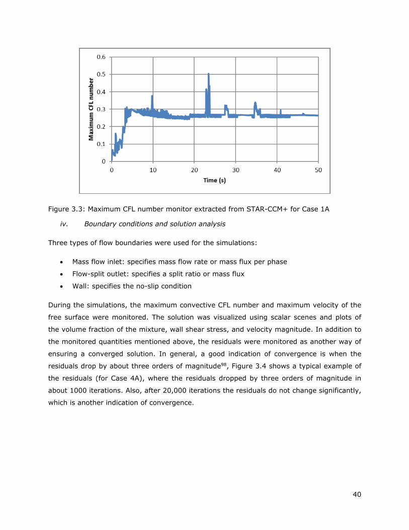
40

Figure 3.3: Maximum CFL number monitor extracted from STAR-CCM+ for Case 1A

iv. Boundary conditions and solution analysis

Three types of flow boundaries were used for the simulations:

Mass flow inlet: specifies mass flow rate or mass flux per phase

Flow-split outlet: specifies a split ratio or mass flux

Wall: specifies the no-slip condition

During the simulations, the maximum convective CFL number and maximum velocity of the

free surface were monitored. The solution was visualized using scalar scenes and plots of

the volume fraction of the mixture, wall shear stress, and velocity magnitude. In addition to

the monitored quantities mentioned above, the residuals were monitored as another way of

ensuring a converged solution. In general, a good indication of convergence is when the

residuals drop by about three orders of magnitude98, Figure 3.4 shows a typical example of

the residuals (for Case 4A), where the residuals dropped by three orders of magnitude in

about 1000 iterations. Also, after 20,000 iterations the residuals do not change significantly,

which is another indication of convergence.

41

Figure 3.4: Example of residuals plot for Case 4A

3.1.1 Model validation

The results are presented in three main categories: depth of flow prediction, wall shear

stress prediction, and velocity profile prediction. The properties of two of the non-

Newtonian, homogeneous mixtures evaluated by Spelay17 are shown in Table 3.2. These

mixtures were tested over a wide range of experimental conditions. For the modelling, a

representative data set, based on the Reynolds number for non-Newtonian fluids, (proposed

by Haldenwang et al.51 and presented here as Equation 2.15) was selected; these conditions

are shown in Table 3.3, the flow rate values were used as boundary conditions. Each

simulation was run for at least for two residence times to ensure development of the flow

solution.

Table 3.2: Rheological properties of the mixtures modelled in this study17

Mixture Density (kg/m3)

𝝉𝒚 (Pa)

k

(Pa.sn)

Power Law Exponent, n

1 1375 34.1 0.0305 1.0

2 1384 7 0.0125 1.0

42

Table 3.3: Experimental conditions considered for modelling in the semi-circular channel

reported by Spelay17

Case* Q (L/s) �̅�

(m/s) Slope (˚)

h1 (m) h2 (m) 𝝉𝒘

(Pa) ReH

(Eq.

2.17)

1A 5.96 0.71 4.5 0.0709 0.0700 39.2 156

1B 3.03 0.40 4.5 0.0647 0.0655 36.1 50

1C 1.27 0.19 4.5 0.0586 0.0592 33.6 12

1D 3.95 0.57 5 0.0607 0.0608 38.4 104

1E 2.02 0.42 6 0.0467 0.0461 37.7 57

2A 2.04 1.67 6 0.0186 0.0172 16.2 2835

2B 3.00 2.12 6 0.0234 0.0207 16.7 4481

2C 2.50 1.08 3 0.0307 0.0255 13.1 1582

2D 2.48 0.78 2 0.038 0.0319 11.1 916

2E 1.54 0.82 3 0.0257 0.0226 11.4 935

2F 2.00 0.66 2 0.0364 0.0310 10.8 669

2G 3.01 1.23 3 0.0322 0.0264 13.3 1984

*Numbers 1 and 2 represent the mixture that was used

i. Depth of flow prediction

For the semi-circular channel, Spelay17 reported depth of flow measurements 7.5 and 13.3

m away from the channel inlet. Consequently, planes were created at these positions for the

simulations; the value for the depth of flow was selected as the position where the volume

fraction of the mixture was 0.5 at the centerline. An example of a scalar scene is shown as

Figure 3.5, which shows the volume fraction distribution of the mixture on a plane

perpendicular to the flow direction; the color blue, occupying most of the upper part of the

channel, represents a mixture volume fraction of 0, whereas the color red, occupying the

bottom part of the channel, represents a mixture volume fraction of 1.0. In addition, a

parity plot between the simulation results and the experiments for the mixtures can be seen

in Figure 3.6.

43

Figure 3.5: Contour plot of the volume fraction of mixture for case 1A in a plane

perpendicular to the flow direction


in Table 3.3.

In Figure 3.6, the parity line (solid line) represents a perfect match between experiments

and simulations, while the dashed lines represent ± 10% of deviation from the parity line as

this was the error percentage reported by Spelay17 for the depth of flow measurements in

his study. Only 3 out of 24 data points are outside this limit, which indicates good

44

agreement between experiments and simulations results. However, there is a trend towards

the prediction of lower depths of flow than what experimentally measured for Mixture # 2.

This is associated with the higher average velocities, with 669 < ReH < 4481, which

contribute to the differences between experiments and predictions for that mixture, because

inertial effects can play a dominant role, causing rippled or wavy surfaces, which were not

considered for the modelling.

In addition, if the data of Figure 3.6 were redistributed using the plane on which they were

measured, as shown in Figure 3.7, it can be seen that there is more scatter when the

measurement was taken 7.5 m (Plane 1) away from the channel inlet when compared to the

measurements made 13.3 m (Plane 2) away from the inlet, regardless of the mixture

properties. This suggests the flow length of 7.5 m is not sufficient to achieve a steady value

of depth of flow for the range of conditions that were tested experimentally. Thus,

subsequent analysis will be made 13.3 m away from the channel inlet.


in Table 3.3.

While experimental uncertainties can influence the discrepancies between experiments and

simulation results, the modelling assumptions must be considered as well. Because there

was no information of the inlet depth of flow required for modelling, it was calculated for

these simulations using the experimental flow rate for each case in Table 3.3. Another

modelling assumption is the fact that, as mentioned in Chapter 2, all phases share the

velocity field when using the VOF model, namely, it does not allow for a no-shear

specification at the interface between the gas phase and liquid phase.

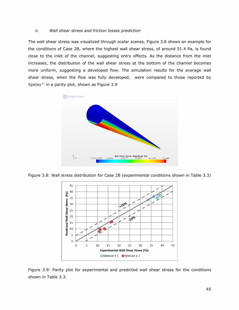
45

ii. Wall shear stress and friction losses prediction

The wall shear stress was visualized through scalar scenes, Figure 3.8 shows an example for

the conditions of Case 2B, where the highest wall shear stress, of around 51.4 Pa, is found

close to the inlet of the channel, suggesting entry effects. As the distance from the inlet

increases, the distribution of the wall shear stress at the bottom of the channel becomes

more uniform, suggesting a developed flow. The simulation results for the average wall

shear stress, when the flow was fully developed, were compared to those reported by

Spelay17 in a parity plot, shown as Figure 3.9

Figure 3.8: Wall stress distribution for Case 2B (experimental conditions shown in Table 3.3)

Figure 3.9: Parity plot for experimental and predicted wall shear stress for the conditions

shown in Table 3.3.

46

From Figure 3.9, it can be seen that all points corresponding to predicted and experimental

wall shear stress are within ± 10% of the parity line, which is the error reported by Spelay17

for the wall shear stress calculations in his study. In contrast with the results in Figure 3.6,

there is no over-prediction of the values for the wall shear stress and there are no clear

distinctions between the mixtures.

iii. Average velocity and velocity profiles prediction

The comparison of predicted and measured average velocity values for the cases in Table

3.3 is shown as Figure 3.10. The predicted average velocity was extracted from a plane

13.3 m away from the channel inlet. Only the cells where the mixture volume fraction was

between 0.5 and 1.0 were considered.

The prediction of the average velocity at a given location is tied to the depth of flow

prediction through the conservation of mass equation. Thus, as expected, the predicted

values for Mixture # 2 seem to deviate more from the parity line compared to those of

Mixture # 1. Spelay17 reported a 4% error in the measurements of the average velocity,

using this criterion, 3 data points can be rejected from Figure 3.10, while the rest shows

good agreement between experiments and simulation results.

Figure 3.10: Parity plot for experimental and predicted average velocity for the conditions

shown in Table 3.3.

Spelay17 also measured local mixture velocities with a Pitot tube. From the cases in Table

3.3, there were data available for local velocities only for cases 2A, 2B, and 2B, because the

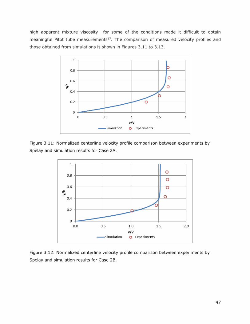
47

high apparent mixture viscosity for some of the conditions made it difficult to obtain

meaningful Pitot tube measurements17. The comparison of measured velocity profiles and

those obtained from simulations is shown in Figures 3.11 to 3.13.


Spelay and simulation results for Case 2A.


Spelay and simulation results for Case 2B.

48


Spelay and simulation results for Case 2G.

Figures 3.11 to 3.13 represent normalized plots of the velocity profiles. On the Y-axis, the

vertical position is normalized using the depth of flow; thus, a value of y/h = 1.0 represents

the location of the free surface. On the X-axis, the local velocity is normalized using the

average velocity. It can be seen that the CFD model can predict the expected trend of the

velocity profiles for a viscoplastic fluid; namely, the velocity is zero at the wall and increases

until it reaches a plug zone, where the shear stress is equal to the yield stress, and the

velocity becomes constant. The prediction for the conditions from Case 2A was in good

agreement with the experimental results. However, while more discrepancies were observed

for the conditions in Cases 2B and 2G, they are less than 10% of difference with respect of

the experiments. These discrepancies can be associated to various reasons: experimental

uncertainties, such as depth of flow measurements; Reynolds numbers near transition-

turbulence, as shown in Table 3.3 Cases 2A, 2B and 2G were evaluated under ReH >1984

conditions, while only laminar effects were considered in the modelling; and the absence of

a correlation in the literature that could account for the yield stress effect on the Pitot tube

measurements, for low Reynolds numbers. Spelay et al.99 assumed a Newtonian fluid of

equivalent apparent viscosity to account for this effect. To further analyze the velocity field

predictions, experiments from other researchers who measured the local mixtures velocities

using a different method are modelled in Section 3.2. This could provide more clarity on the

roots of the discrepancies between the experiments and simulations.

49

iv. Friction losses

As described in Section 2.3.1, Burger et al.53 proposed a correlation to predict the Fanning

friction factor using the Reynolds number for non-Newtonian fluids, and different channel

geometries. Specifically, for a semi-circular channel, the correlation is presented here as

Equation 2.20

𝑓 = 0.048𝑅𝑒−0.2049 + (16.2𝑅𝑒−1 − 0.048𝑅𝑒−0.2049)

(1 + (𝑅𝑒1055

)230

)

0.015 (2.20)

In addition, as a reminder, the Fanning friction factor and the non-Newtonian Reynolds

number are given by

𝑓 =2𝜏𝑤𝜌�̅�2

= 2𝑅ℎ𝑔 sin 𝜃

�̅�2 (2.16)

𝑅𝑒𝐻 = 8𝜌𝑉2

𝜏𝑦 + 𝑘 (2𝑉𝑅ℎ)𝑛 (2.15)

The simulation results were used to calculate the Reynolds numbers and the friction factors,

described by Equations 2.15 and 2.16, and then compared against Equation 2.20, shown as

a Moody diagram in Figure 3.14.

Figure 3.14: Comparison of the simulation results and Fanning friction factor correlation by

Burger et al.53

50

From Figure 3.14, it can be seen that when ReH < 2000, there is close agreement between

simulations and the predictions of Eq. (2.20). This range covers the laminar flow regime

(ReH ≤ 1000), and transition regimes (1000 < ReH ≤ 2000). For ReH > 2000, there is poorer

agreement between the simulation results and the predictions of Eq. (2.20), because inertial

effects were not considered during the modelling. This comparison helps to further validate

the model for ReH < 2000 values.

3.2 Rectangular channel

As discussed before, the purpose of these simulations is to study the uncertainties seen in

the velocity profile predictions for Cases 2A, 2B, and 2G. Specifically, the role of inertial

effects at high Reynolds numbers and the assumptions made to measure the local velocity

using a Pitot tube, are studied. To address this, the laminar experimental conditions of

Haldenwang et al.45 were modelled. They used an Ultrasonic Velocity Profiling (UVP) system

to measure the local mixture velocity and the laminar sheet flow model proposed by De Kee

et al.44 to study the flow of Power Law and Bingham Plastic fluids in a rectangular flume,

which was 300 mm in width and 10 m in length. A schematic representation of their setup is

shown as Figure 3.15.

Figure 3.15: Schematic of rectangular flume used by Haldenwang et al.45 available under a

Creative Commons Attibution Licence

The meshing technique was directed meshing, which resulted in a mesh structure of 46780

cells, shown as Figure 3.16. With respect to the physics of the problem, the same STAR-

CCM+ models, shown in Table 3.1, were used with the distinction that the temporal

discretization was steady.

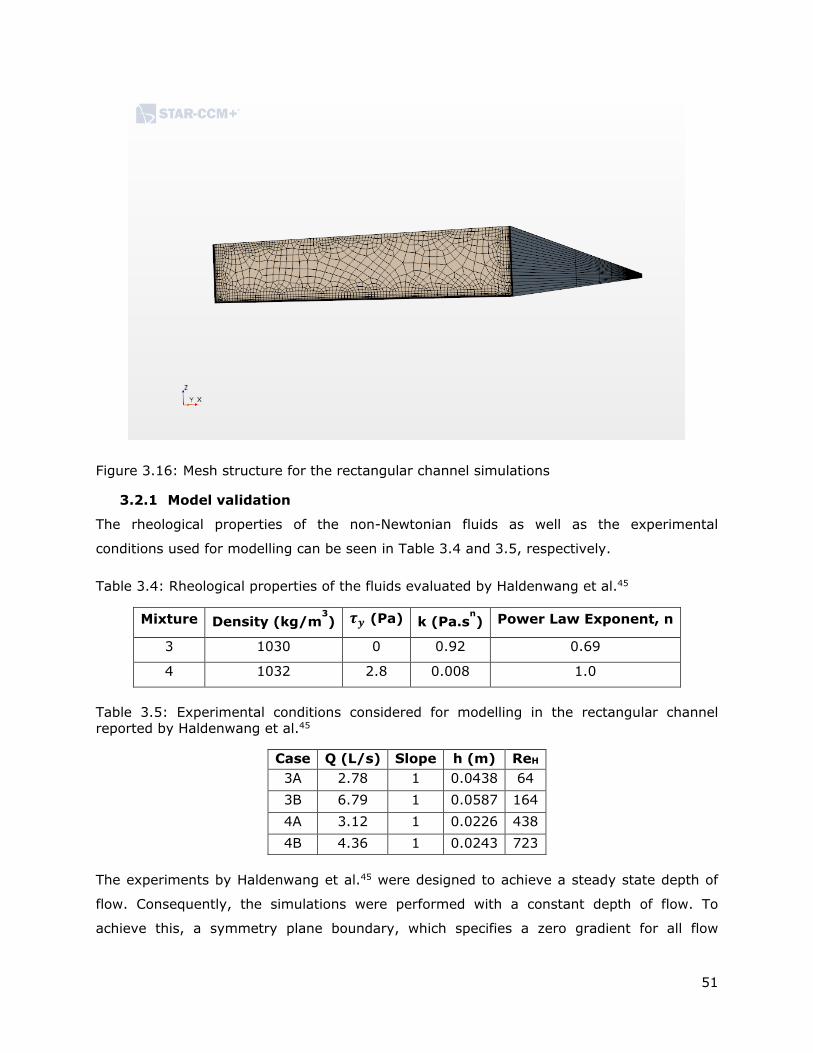
51

Figure 3.16: Mesh structure for the rectangular channel simulations


The rheological properties of the non-Newtonian fluids as well as the experimental

conditions used for modelling can be seen in Table 3.4 and 3.5, respectively.

Table 3.4: Rheological properties of the fluids evaluated by Haldenwang et al.45

Mixture Density (kg/m3) 𝝉𝒚 (Pa) k (Pa.s

n) Power Law Exponent, n

3 1030 0 0.92 0.69

4 1032 2.8 0.008 1.0

Table 3.5: Experimental conditions considered for modelling in the rectangular channel reported by Haldenwang et al.45

Case Q (L/s) Slope h (m) ReH

3A 2.78 1 0.0438 64

3B 6.79 1 0.0587 164

4A 3.12 1 0.0226 438

4B 4.36 1 0.0243 723

The experiments by Haldenwang et al.45 were designed to achieve a steady state depth of

flow. Consequently, the simulations were performed with a constant depth of flow. To

achieve this, a symmetry plane boundary, which specifies a zero gradient for all flow

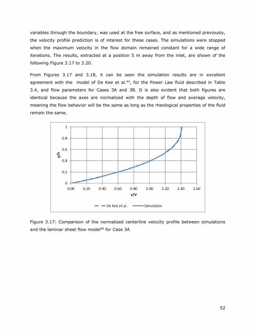
52

variables through the boundary, was used at the free surface, and as mentioned previously,

the velocity profile prediction is of interest for these cases. The simulations were stopped

when the maximum velocity in the flow domain remained constant for a wide range of

iterations. The results, extracted at a position 5 m away from the inlet, are shown of the

following Figure 3.17 to 3.20.

From Figures 3.17 and 3.18, it can be seen the simulation results are in excellent

agreement with the model of De Kee et al.44, for the Power Law fluid described in Table

3.4, and flow parameters for Cases 3A and 3B. It is also evident that both figures are

identical because the axes are normalized with the depth of flow and average velocity,

meaning the flow behavior will be the same as long as the rheological properties of the fluid

remain the same.


and the laminar sheet flow model44 for Case 3A

53


and the laminar sheet flow model44 for Case 3B

Likewise, Figures 3.19 and 3.20 show that the simulation results for the viscoplastic fluid

are consistent with the predictions from the model of De Kee et al.44 for the normalized

centerline velocity profiles. However, contrary to what was seen with Power Law fluids, the

normalized plots do not necessarily collapse on one single curve. This is because increasing

the flow rate changes the location of the surface that separates the sheared and the plug

regions; the sheared region increases while the plug region decreases with increasing flow

rate. This surface is located at y/h values of 0.3 and 0.35, for cases 4A and 4B,

respectively.

Given these results, a comparison between the predicted velocity profiles for the semi-

circular and the rectangular channel can be made. For the conditions evaluated by

Haldenwang et al.45 the v/V values at the core range from 1.11 to 1.13, whereas for Cases

2A, 2B, and 2G (from Spelay17) the v/V values range from 1.37 to 1.68. These remarkable

differences can be attributed to wall effects, and higher flow rates leading to transition or

turbulence. However, it is difficult to make a direct comparison between both sets of

experimental data because the mixtures properties (as shown in Tables 3.1 and 3.5), the

geometries of the channels, and the purpose of the studies were different. More studies on

this matter are needed to confirm the root of the differences.

54

Figure 3.19: Comparison of the normalized centerline velocity profile between simulations and the laminar sheet flow model44 for Case 4A


and the laminar sheet flow model44 for Case 4B.

3.3 Modelling limitations

The models are limited to laminar flow regime. It was shown that including

conditions in the transition or turbulent regime can lead to discrepancies between

experiments and simulations

The VOF model in STAR-CCM+ assumes a shared velocity, temperature, and

pressure fields for all phases which has implications on how the data is extracted

55

from the solution; the volume fraction of the mixture from 0.5 to 1.0 is used as a

condition to extract the velocity field corresponding to the mixture.

The model is restricted to homogeneous mixtures. The VOF model can be coupled

with LMP to include particle phases. However, this approach cannot be used for

concentrated suspensions as those shown in Chapter 4 and 5. In order to study

those suspensions, the Multiphase Segregated Flow, also known Eulerian Multiphase

will be used

3.4 Conclusions

A numerical model was developed using STAR-CCM+ to predict the behavior of non-

Newtonian mixtures flowing in a semi-circular flume under laminar flow. The model

can predict depth of flow, and wall shear stress within 10% of difference, and

average velocity within 4% of difference, when compared with the experimental

data from Spelay17

The Fanning friction factor was calculated from the simulation results, and then was

compared along with the Reynolds number in a Moody diagram using the correlation

by Burger et al.53 with excellent agreement

The simulated velocity profiles were compared with those measured by Spelay17.

While the expected trend for a viscoplastic fluid was seen, there were some

discrepancies between prediction and experiments. This could be attributed to

experimental uncertainties on the Pitot tube measurements, transition-to-turbulent

flow regimes, and VOF modelling assumptions

To further study the discrepancies surrounding the velocity profile predictions, the

experimental conditions by Haldenwang et al.45 were considered. These consisted of

non-Newtonian mixtures flowing in a rectangular flume under laminar flow. In

contrast to Spelay17, they used UVP as the method to measure local velocity which

was validated using the laminar sheet flow model44. The simulation results were in

close agreement with the prediction of the model by De Kee et al.44. Furthermore, a

comparison between the simulation results of the semi-circular and rectangular

channel showed that the normalized velocity distribution at the core for the cases in

the semi-circular channel were up to 48% higher than those in the rectangular

channel, suggesting inertial or wall effects were present. However, it is difficult to

make a direct comparison given that the mixture properties, geometries, and

purpose of the studies were different.

56

3.5 Recommendations

In order to improve the consistency, accuracy, and the stability of the model the following

activities are recommended:

Perform reliable, high-quality measurements of local velocities of viscoplastic fluids

flowing through an open channel. A comparison with additional experimental data,

maintaining ReH < 1000 and using mixtures with a wide range of yield stresses, for

example 2-40 Pa, could help to address some of the discrepancies observed in some

of the modelling results. In addition, if a Pitot tube is used in conjunction with

another measurement method, such as UVP, one could validate or disprove the

assumptions made for the Pitot tube local velocity measurements for viscoplastic

fluids

Study the ability of the Multiphase segregated model, described in Section 2.6.2, to

model the homogeneous, laminar, open-channel flow of non-Newtonian fluids. This

will allow to study the air and mixture phases separately and make it easier for the

user to extract the desired results

Although an informal grid refinement study was performed, it is recommended to

study the grid dependence of the results in more depth

57

4. Fluid-particle systems – preliminary studies

The purpose of this chapter is to present the results of a preliminary modelling study of

fluid-particle systems using STAR-CCM+ to test its ability to predict characteristic

phenomena of suspensions: shear-induced migration, quasi-static settling, and the laminar

transport of settling slurries. Three modeling scenarios are considered, as each provides the

opportunity to focus on a different mechanism.

4.1 Shear-induced migration

As mentioned in Chapter 2, particles tend to travel from high shear rate to lower shear rate

zones, causing heterogeneities in the particle volume fraction distribution28. For this case,

the experimental conditions described by Hampton et al.29 were modelled. They studied the

shear-induced migration of neutrally-buoyant particles in a tube by measuring the local

particle volume fraction and axial velocity using nuclear magnetic resonance (NMR) as

shown in Figure 4.1.

Figure 4.1: (a) Schematic of the experimental setup (b) Superconducting 1.9 T magnet29


The flow domain consisted of a circular tube that was 50.8 mm of diameter and was up to

40 m in length to match the experiments of Hampton et al.29. The meshing approach was

directed meshing and the cell count ranged from 6500 to 9000, with a base cell size of 4

mm, bigger than the smallest particle in the flow domain. The mesh structure is shown in

Figure 4.2.

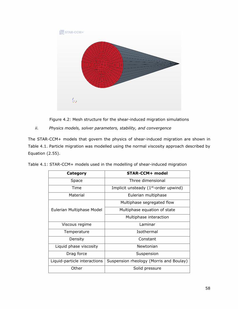
58

Figure 4.2: Mesh structure for the shear-induced migration simulations

ii. Physics models, solver parameters, stability, and convergence

The STAR-CCM+ models that govern the physics of shear-induced migration are shown in

Table 4.1. Particle migration was modelled using the normal viscosity approach described by

Equation (2.55).

Table 4.1: STAR-CCM+ models used in the modelling of shear-induced migration



Time Implicit unsteady (1st-order upwind)

Material Eulerian multiphase


Multiphase segregated flow

Multiphase equation of state

Multiphase interaction



Density Constant

Liquid phase viscosity Newtonian

Drag force Suspension

Liquid-particle interactions Suspension rheology (Morris and Boulay)

Other Solid pressure

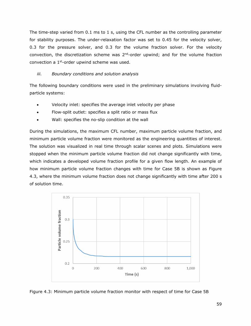
59

The time-step varied from 0.1 ms to 1 s, using the CFL number as the controlling parameter

for stability purposes. The under-relaxation factor was set to 0.45 for the velocity solver,

0.3 for the pressure solver, and 0.3 for the volume fraction solver. For the velocity

convection, the discretization scheme was 2nd-order upwind; and for the volume fraction

convection a 1st-order upwind scheme was used.

iii. Boundary conditions and solution analysis

The following boundary conditions were used in the preliminary simulations involving fluid-

particle systems:

Velocity inlet: specifies the average inlet velocity per phase


Wall: specifies the no-slip condition at the wall

During the simulations, the maximum CFL number, maximum particle volume fraction, and

minimum particle volume fraction were monitored as the engineering quantities of interest.

The solution was visualized in real time through scalar scenes and plots. Simulations were

stopped when the minimum particle volume fraction did not change significantly with time,

which indicates a developed volume fraction profile for a given flow length. An example of

how minimum particle volume fraction changes with time for Case 5B is shown as Figure

4.3, where the minimum volume fraction does not change significantly with time after 200 s

of solution time.

Figure 4.3: Minimum particle volume fraction monitor with respect of time for Case 5B

60


The experimental conditions modelled in this study are shown in Table 4.2, the average

velocity and the bulk particle volume fraction were used as boundary conditions. The solid

particle phase was modelled as monodisperse.

Table 4.2: Experimental conditions modelled for shear-induced migration29

Case �̅�

(m/s)

d

(mm)

μf

(Pa.s)

ρf

(kg/m3) 𝝓𝒔,𝒃𝒖𝒍𝒌

5A 0.1 3.175 2.1 1180.7 0.2

5B 0.1 3.175 2.1 1180.7 0.3

5C 0.1 3.175 2.1 1180.7 0.45

The scalar scenes of the developed particle volume fraction and velocity profiles for case 5B

are shown as Figure 4.4 and 4.5. They show the model can predict shear-induced particle

migration in a tube, namely, particles migrate towards the center of the tube because of the

gradients in velocity. The particle volume fraction and velocity profiles from the cases in

Table 4.2. are compared with experimental data from Hampton et al.29, shown in Figures

4.6 to 4.11. The solution time was around 2000 s for Case 5A, 1000 s for Case 5B, and

3500 s for Case 5C. Each simulation was completed in 1 to 4 hours.

Figure 4.4: Contour plot of the particle volume fraction for Case 5B in a plane perpendicular

to the flow direction

61

Figure 4.5: Contour plot of the carrier fluid velocity for Case 5B in a plane perpendicular to

the flow direction


experiments by Hampton et al.29 for Case 5A

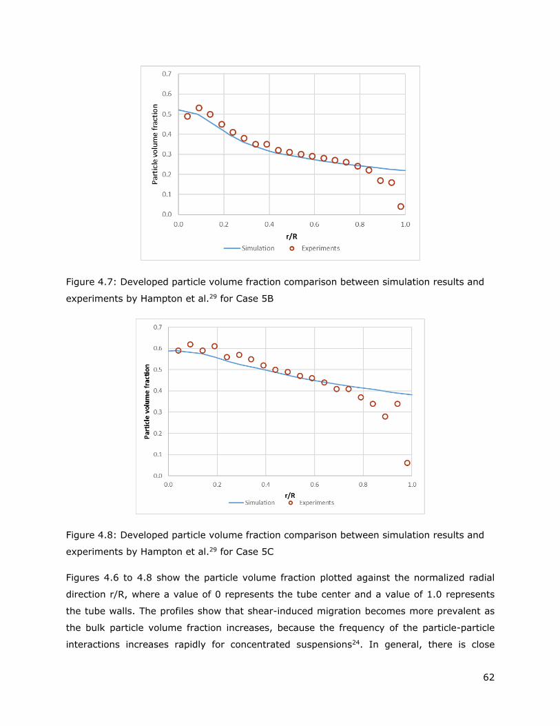
62


experiments by Hampton et al.29 for Case 5B


experiments by Hampton et al.29 for Case 5C

Figures 4.6 to 4.8 show the particle volume fraction plotted against the normalized radial

direction r/R, where a value of 0 represents the tube center and a value of 1.0 represents

the tube walls. The profiles show that shear-induced migration becomes more prevalent as

the bulk particle volume fraction increases, because the frequency of the particle-particle

interactions increases rapidly for concentrated suspensions24. In general, there is close

63

agreement between simulations and experiments for 0.2 ≤ r/R ≤ 0.8. However, the model

is unable to predict a decrease in volume fraction near the wall as was found in the

experiments. To further analyze these discrepancies, additional evaluations were

performed: the resolution of the mesh was improved at the wall to study a potential effect

on the numerical solution; the length of the tube was increased to up to 110 m, in case the

simulated flow length was not sufficient to fully develop the particle volume fraction profiles;

the time-step was decreased to evaluate its effect on the numerical solution; the lift force,

which is experienced by particles and is perpendicular to the relative velocity field, was

added as additional physics to the modelling. Also, the wall lubrication force model was

added. As described in Section 2.6.2, this model is used to prevent bubbles from touching

the walls100, STAR-CCM+ does not provide a similar built-in model to study wall collision for

solid spheres in an Eulerian or continuum framework. None of the approaches mentioned

above had a significant effect on the developed particle volume fraction profiles shown in

Figures 4.6 to 4.8. Also, Hampton et al.29 compared their experimental results with the

model of Phillips et al. 30, described in Section 2.4.2, and noticed the same limitations; in

fact, the predicted values obtained using the Phillips et al. 30 model at the wall for the cases

shown in Figures 4.6 to 4.8 are very similar to those predicted by the model presented here.

Thus, it is recommended that additional particle-level studies, such as with the use of DEM,

be conducted to study wall collisions in more detail and improve the suspension rheology

model. Although this is beyond the scope of this project, for a recent study on this subject

the reader is referred to the work of Tomac and Gutierrez101.


experiments by Hampton et al.29 for Case 5A

64


experiments by Hampton et al.29 for Case 5B


experiments by Hampton et al.29 for Case 5C

Figures 4.9 to 4.11 show a comparison between the simulated and experimental velocity

profiles. In these plots, the local velocity was normalized using the average velocity and

plotted against the normalized radial distance, r/R. There is close agreement between

experiments and simulation results for cases 5A and 5B. For case 5C, where the bulk

particle volume fraction is 0.45, there is more scatter in the experimental data because the

higher particle concentration causes an increase in particle-particle interactions, such as

collisions, which causes more (and stronger) fluctuations in the local velocity

65

measurements. It is also shown that the velocity profiles become blunter, i.e. v/V values at

the center of the tube start to decrease as the bulk particle concentration increases. This

effect is a consequence of the mixture viscosity increase with increasing particle volume

fraction.

As the particle volume fraction increases, the entrance length (L/D), necessary to achieve

fully developed profiles for the velocity and particle volume fraction, decreases rapidly,

which is consistent with the results reported by Hampton et al.29, shown in Table 4.3. In

addition, the simulated average wall shear stress is shown in Table 4.3; even though these

were not reported by Hampton et al.29, it can be seen that an increase in the particle bulk

volume fraction from 0.3 to 0.45 increases the average wall shear stress by 130 % which

has implications on the energy requirements to transport these suspensions.

Furthermore, it should be noted that STAR-CCM+ struggled with stability in the simulations

where the particle volume fraction anywhere in the flow domain approached the maximum

packing volume fraction. As mentioned in Chapter 2, most numerical methods become

limited when maximum packing is approached.

Table 4.3: Experimental entrance length and simulated average wall shear stress for cases

in Table 4.2

𝝓𝒔,𝒃𝒖𝒍𝒌 Entrance length (L/D)29 Average wall shear stress (Pa)

0.2 785 46

0.3 183 60

0.45 42 139

4.2 Single-particle settling in viscoplastic fluids

The settling of a falling sphere through a viscoplastic fluid35 is modelled. The experimental

study consisted on spheres being thrown from the top of a settling column. Several

viscoplastic mixtures were used with yield stress values ranging from 1.3 to 30 Pa. Different

types of spheres (ceramic, steel, and aluminum) with diameters ranging from 12.7 to 19

mm and densities from 2710 to 7841 kg/m3 were used. The settling velocities of the spheres

were measured using Electrical Impedance Tomography (EIT). With that information, a

correlation was developed to predict the terminal velocity of spheres as described in Chapter

2. A schematic representation of the settling column is shown as Figure 4.12.

66

Figure 4.12: Schematic representation of the settling column used by Shokrollahzadeh35


The geometry was created to be two dimensional and was 101.6 in width and 1.5 in height.

This resulted in a mesh structure with 1120 quadrilateral cells, as shown in Figure 4.13.


The main STAR-CCM+ models used for the description of the physics of single-particle

settling in viscoplastic fluids are shown in Table 4.3. The Lagrangian Multiphase model

(LMP) was used to model the solid particle phase, for better visualization and tracking of the

particle phase.

Table 4.4: STAR-CCM+ models used in the single-particle settling simulations


Space Two dimensional


Material Lagrangian multiphase

Eulerian multiphase (2nd-order upwind)



Density Constant

Other Gravity

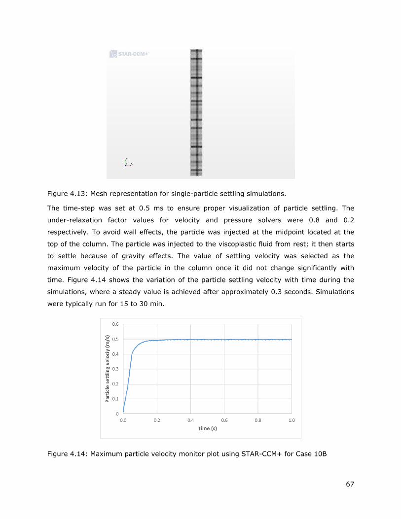
67

Figure 4.13: Mesh representation for single-particle settling simulations.

The time-step was set at 0.5 ms to ensure proper visualization of particle settling. The

under-relaxation factor values for velocity and pressure solvers were 0.8 and 0.2

respectively. To avoid wall effects, the particle was injected at the midpoint located at the

top of the column. The particle was injected to the viscoplastic fluid from rest; it then starts

to settle because of gravity effects. The value of settling velocity was selected as the

maximum velocity of the particle in the column once it did not change significantly with

time. Figure 4.14 shows the variation of the particle settling velocity with time during the

simulations, where a steady value is achieved after approximately 0.3 seconds. Simulations

were typically run for 15 to 30 min.

Figure 4.14: Maximum particle velocity monitor plot using STAR-CCM+ for Case 10B

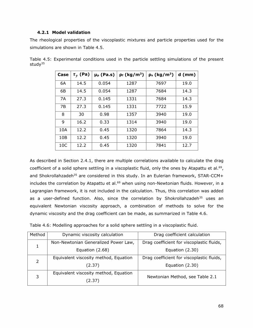
68


The rheological properties of the viscoplastic mixtures and particle properties used for the

simulations are shown in Table 4.5.

Table 4.5: Experimental conditions used in the particle settling simulations of the present

study35

Case 𝝉𝒚 (Pa) μp (Pa.s) ρf (kg/m3) ρs (kg/m3) d (mm)

6A 14.5 0.054 1287 7697 19.0

6B 14.5 0.054 1287 7684 14.3

7A 27.3 0.145 1331 7684 14.3

7B 27.3 0.145 1331 7722 15.9

8 30 0.98 1357 3940 19.0

9 16.2 0.33 1314 3940 19.0

10A 12.2 0.45 1320 7864 14.3

10B 12.2 0.45 1320 3940 19.0

10C 12.2 0.45 1320 7841 12.7

As described in Section 2.4.1, there are multiple correlations available to calculate the drag

coefficient of a solid sphere settling in a viscoplastic fluid, only the ones by Atapattu et al.69,

and Shokrollahzadeh35 are considered in this study. In an Eulerian framework, STAR-CCM+

includes the correlation by Atapattu et al.69 when using non-Newtonian fluids. However, in a

Lagrangian framework, it is not included in the calculation. Thus, this correlation was added

as a user-defined function. Also, since the correlation by Shokrollahzadeh35 uses an

equivalent Newtonian viscosity approach, a combination of methods to solve for the

dynamic viscosity and the drag coefficient can be made, as summarized in Table 4.6.

Table 4.6: Modelling approaches for a solid sphere settling in a viscoplastic fluid.

Method Dynamic viscosity calculation Drag coefficient calculation

1 Non-Newtonian Generalized Power Law,

Equation (2.68)

Drag coefficient for viscoplastic fluids,

Equation (2.30)

2 Equivalent viscosity method, Equation

(2.37)

Drag coefficient for viscoplastic fluids,

Equation (2.30)

3 Equivalent viscosity method, Equation

(2.37) Newtonian Method, see Table 2.1

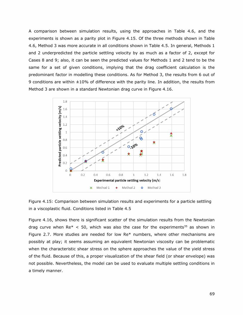
69

A comparison between simulation results, using the approaches in Table 4.6, and the

experiments is shown as a parity plot in Figure 4.15. Of the three methods shown in Table

4.6, Method 3 was more accurate in all conditions shown in Table 4.5. In general, Methods 1

and 2 underpredicted the particle settling velocity by as much as a factor of 2, except for

Cases 8 and 9; also, it can be seen the predicted values for Methods 1 and 2 tend to be the

same for a set of given conditions, implying that the drag coefficient calculation is the

predominant factor in modelling these conditions. As for Method 3, the results from 6 out of

9 conditions are within ±10% of difference with the parity line. In addition, the results from

Method 3 are shown in a standard Newtonian drag curve in Figure 4.16.

Figure 4.15: Comparison between simulation results and experiments for a particle settling

in a viscoplastic fluid. Conditions listed in Table 4.5

Figure 4.16, shows there is significant scatter of the simulation results from the Newtonian

drag curve when Re* < 50, which was also the case for the experiments35 as shown in

Figure 2.7. More studies are needed for low Re* numbers, where other mechanisms are

possibly at play; it seems assuming an equivalent Newtonian viscosity can be problematic

when the characteristic shear stress on the sphere approaches the value of the yield stress

of the fluid. Because of this, a proper visualization of the shear field (or shear envelope) was

not possible. Nevertheless, the model can be used to evaluate multiple settling conditions in

a timely manner.

70

Figure 4.16: Comparison between simulation results and the Newtonian drag curve

4.3 Laminar transport of coarse particles

The transport of negatively-buoyant particles was also studied. This combines the effects of

shear-induced migration and hindered-particle settling. The experimental studies by Gillies

et al.32 were modelled. Their setup consisted of a 50 mm (diameter) loop where sand

suspended in a Newtonian oil was circulated, shown here as Figure 4.17. They measured

solid concentration distribution, using a gamma ray densitometer; velocity distribution,

using a constant-temperature hot-film anemometer; as well as pressure gradients.

Figure 4.17: The 50 mm pipeflow loop used in the experiments by Gillies et al.32 where: d)

Gamma ray densitometer, g) Glass observation section, h) Heat Exchanger, a) Hot film

anemometer, s) Sampler, T) Temperature sensor, V) Acrylic observation section

71


The pipe was 52.5 mm in diameter and was 30 and 60 m in length for Cases shown in Table

4.7. The meshing approach was direct meshing, resulting in mesh structures with 6500 and

19000 cells for Cases 11A and 11B, respectively. The mesh structure for Case 11A is shown

as Figure 4.18.

Figure 4.18: Mesh structure used in the laminar transport of coarse particles simulations


The STAR-CCM+ models used to describe the physics involved in the laminar transport of

coarse particles are the same as those shown in Table 4.1, with the addition of the gravity

force model for negatively-buoyant particles.

The time-step varied from 0.01 ms to 0.5 s, and was determined by monitoring the CFL

number in the fluid domain. The under-relaxation factors were 0.27 for the velocity solver,

0.1 for the pressure solver, and 0.1 for the volume fraction solver. The simulations were

stopped when the maximum particle volume fraction and the particle volume fraction profile

did not change significantly with time.


The experimental conditions that were modelled are shown in Table 4.7. Preliminary

simulations were performed to choose the expression of relative viscosity that best

represented the experimental behaviour. As mentioned before, Equations (2.45) and (2.47)

are built-in within STAR-CCM+, whereas Equation (2.48) was introduced as a user-defined

function. The results showed that Equation (2.47), proposed by Morris and Boulay27,

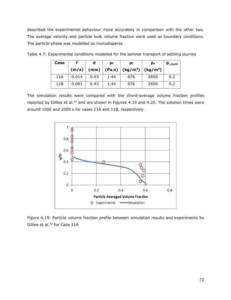
72

described the experimental behaviour more accurately in comparison with the other two.

The average velocity and particle bulk volume fraction were used as boundary conditions.

The particle phase was modelled as monodisperse

Table 4.7: Experimental conditions modelled for the laminar transport of settling slurries

Case �̅�

(m/s)

d

(mm)

μf

(Pa.s)

ρf

(kg/m3)

ρs

(kg/m3)

𝝓𝒔,𝒃𝒖𝒍𝒌

11A 0.014 0.43 1.44 876 2650 0.2

11B 0.061 0.43 1.44 876 2650 0.2

The simulation results were compared with the chord-average volume fraction profiles

reported by Gillies et al.32 and are shown in Figures 4.19 and 4.20. The solution times were

around 1000 and 2000 s for cases 11A and 11B, respectively.


Gillies et al.32 for Case 11A

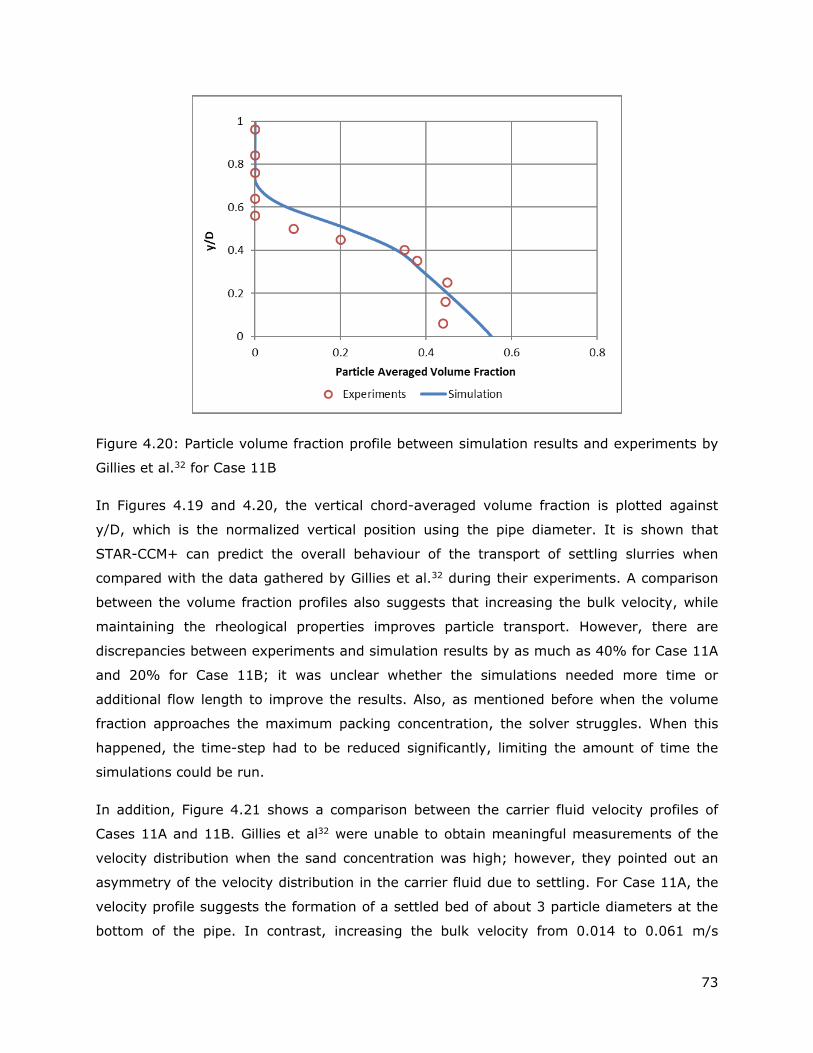
73


Gillies et al.32 for Case 11B

In Figures 4.19 and 4.20, the vertical chord-averaged volume fraction is plotted against

y/D, which is the normalized vertical position using the pipe diameter. It is shown that

STAR-CCM+ can predict the overall behaviour of the transport of settling slurries when

compared with the data gathered by Gillies et al.32 during their experiments. A comparison

between the volume fraction profiles also suggests that increasing the bulk velocity, while

maintaining the rheological properties improves particle transport. However, there are

discrepancies between experiments and simulation results by as much as 40% for Case 11A

and 20% for Case 11B; it was unclear whether the simulations needed more time or

additional flow length to improve the results. Also, as mentioned before when the volume

fraction approaches the maximum packing concentration, the solver struggles. When this

happened, the time-step had to be reduced significantly, limiting the amount of time the

simulations could be run.

In addition, Figure 4.21 shows a comparison between the carrier fluid velocity profiles of

Cases 11A and 11B. Gillies et al32 were unable to obtain meaningful measurements of the

velocity distribution when the sand concentration was high; however, they pointed out an

asymmetry of the velocity distribution in the carrier fluid due to settling. For Case 11A, the

velocity profile suggests the formation of a settled bed of about 3 particle diameters at the

bottom of the pipe. In contrast, increasing the bulk velocity from 0.014 to 0.061 m/s

74

increases the particle transport to the extent that there is no formation of a settled bed, as

shown by the velocity profile for case 11B. The simulated pressure drops were 650 Pa and

3000 Pa, whereas the ones reported by Gillies et al.32 were 800 Pa and 2900 Pa for the

conditions simulated in cases 11A and 11B.

Figure 4.21: Simulated velocity profiles for Cases 11A and 11B

The goal of the studies presented in this chapter was to model characteristic phenomena of

suspensions involved in the subsequent modelling stages of the present study; i.e. shear-

induce migration, single-particle settling in viscoplastic fluids, and the laminar pipeline

transport of settling slurries. Experimental studies where each mechanism could be studied

separately were chosen. For the shear-induce migration modelling, it was shown that by

using the “normal viscosity” approach, proposed by Morris and Boulay27, the model captures

the overall behaviour of particles migrating towards the center of a tube due to shear rate

gradients. However, the model is unable to account for particle-wall collisions. The extent

to which this lack of particle-wall interaction can affect particle settling modelling is

unknown; numerical, particle-level studies can be done to improve the predictions of the

model. Single-particle settling of a sphere in a viscoplastic fluid was modelled using

experimental conditions from Shokrollahzadeh’s35 study. Two correlations for the calculation

of the drag coefficient were considered35,69, it was determined that the one proposed by

Atapattu et al.69 underpredicted the experimental results in all cases; the correlation

proposed by Shokrollahzadeh35 produced better simulation results when compared with the

75

experimental data. However, care should be taken when using this correlation as it assumes

an equivalent Newtonian viscosity to account for the viscosity of the viscoplastic fluid, and

its results deviate considerably from a Newtonian drag curve when Re* < 50. For the

laminar pipeline transport of settling slurries, the studies by Gillies et al32 were modelled.

While the model predicts the overall behaviour of particle settling, there were discrepancies

between simulations and experiments of up to 40%, it is unclear if more time or longer

pipes were needed to refine the results. The simulated pressure gradients were within 20%

of difference for Case 11A and 4% for Case 11B.

4.4 Modelling limitations

The suspension rheology model is unable to predict a decrease in the particle volume

fraction at the wall to the extent the experiments by Hampton et al.29 showed for the

shear-induced migration of neutrally buoyant particles suspended in a Newtonian

fluid

The STAR-CCM+ solver struggled with stability of the simulation when the volume

fraction within the flow domain approached the maximum packing concentration,

requiring a significant decrease in time-step, limiting the amount of time each

simulation could be run

The built-in mesh generation models in STAR-CCM+ only allowed for tube lengths up

to 115 m

The drag force calculation in a Lagrangian framework within STAR-CCM+ does not

allow to introduce non-Newtonian behaviour on its calculation, which requires the

use of UDFs to account for this effect

The model developed for the study of single-particle settling in viscoplastic fluids

uses Shokrollahzadeh’s35 approach to calculate for an equivalent Newtonian

viscosity. Thus, it suffers from the same limitations as the correlation and deviates

significantly from the Newtonian drag curve when Re* < 50

4.5 Conclusions

A numerical model was developed to study the shear-induced migration of neutrally

buoyant particles suspended in a Newtonian Fluid, which was successfully compared

with experimental data by Hampton et al.29

There was good agreement between the simulated velocity profiles and the

experiments, for all cases

There were discrepancies on the particle volume fraction predictions as r/R > 0.8, for

all cases

76

A numerical model to study particle settling of a sphere in viscoplastic fluids was

developed and compared successfully with available experimental data by

Shokrollahzadeh35

There is significant scatter of the particle settling velocity results and the Newtonian

drag curve for Re* < 50

A numerical model was developed to study the laminar transport of settling slurries

and compared successfully with experimental data

There model was able to capture the overall behaviour as seen in the experiments by

Gillies et al.32. However, there were discrepancies between simulation results and

experiments. This is related with the instability of the model when solving the flow

when maximum packing is reached in the flow domain

The simulated velocity profiles showed the formation of a settled bed at the bottom

of the pipe and asymmetry between the upper and lower half because of the effect of

particle settling. Increasing the bulk velocity improves particle transport under

laminar flow conditions to the extent that the settled bed disappears

For two different cases, the simulated pressure gradients were within 20% and 4%

of difference when compared with the experiments

4.6 Recommendations

The following studies are recommended to expand the reliability of the model and improve

our understanding of the physics:

Study in more detail the wall effects on particle volume fraction profiles of neutrally

buoyant particle in a tube. DEM studies can be done to account for particle wall

collisions. This could aid in the development of models that account accurately for

particle-wall collisions.

Validate the single-particle settling model using data from studies with Power Law

fluids and Herschel-Bulkley fluids to further study the effect of the yield stress in

particle settling

Study the mechanism(s) that govern particle settling in viscoplastic fluids at Re* <

50

77

5. Laminar, open-channel flow of non-Newtonian

suspensions

Recall that the main goal of this project is to model the settling behaviour of monodisperse

coarse particles, suspended in a non-Newtonian fluid flowing under laminar, open-channel

flow conditions. The experimental data from Spelay17 were used for validation of the CFD

model; a description of his experimental setup is shown in Chapter 3.

Preliminary modelling studies with three Eulerian phases (i.e. carrier fluid-coarse particle-air

phases) proved to be more challenging than expected. A single simulation could take weeks

or months because of the small time-steps required to archive stability of the solver. Thus,

the focus was shifted to the study of particle settling only; in other words, the simulations

were set up using a constant depth of flow. This allowed for faster simulations because the

air phase was not considered into the calculations.


The same semi-circular channel as described in Section 3.1 was modelled, with the

distinction that the channel was truncated to match a constant depth of flow throughout the

channel for each condition. Likewise, the meshing technique was directed meshing, resulting

in approximately 27000 cells. A schematic of the mesh is shown as Figure 5.1.

Figure 5.1: Mesh structure used for non-Newtonian suspension simulations

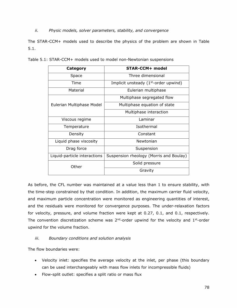
78

ii. Physic models, solver parameters, stability, and convergence

The STAR-CCM+ models used to describe the physics of the problem are shown in Table

5.1.

Table 5.1: STAR-CCM+ models used to model non-Newtonian suspensions




Material Eulerian multiphase


Multiphase segregated flow

Multiphase equation of state

Multiphase interaction



Density Constant

Liquid phase viscosity Newtonian

Drag force Suspension

Liquid-particle interactions Suspension rheology (Morris and Boulay)

Other Solid pressure

Gravity

As before, the CFL number was maintained at a value less than 1 to ensure stability, with

the time-step constrained by that condition. In addition, the maximum carrier fluid velocity,

and maximum particle concentration were monitored as engineering quantities of interest,

and the residuals were monitored for convergence purposes. The under-relaxation factors

for velocity, pressure, and volume fraction were kept at 0.27, 0.1, and 0.1, respectively.

The convention discretization scheme was 2nd-order upwind for the velocity and 1st-order

upwind for the volume fraction.

iii. Boundary conditions and solution analysis

The flow boundaries were:

Velocity inlet: specifies the average velocity at the inlet, per phase (this boundary

can be used interchangeably with mass flow inlets for incompressible fluids)


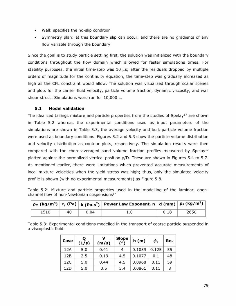
79

Wall: specifies the no-slip condition

Symmetry plan: at this boundary slip can occur, and there are no gradients of any

flow variable through the boundary

Since the goal is to study particle settling first, the solution was initialized with the boundary

conditions throughout the flow domain which allowed for faster simulations times. For

stability purposes, the initial time-step was 10 s; after the residuals dropped by multiple

orders of magnitude for the continuity equation, the time-step was gradually increased as

high as the CFL constraint would allow. The solution was visualized through scalar scenes

and plots for the carrier fluid velocity, particle volume fraction, dynamic viscosity, and wall

shear stress. Simulations were run for 10,000 s.

5.1 Model validation

The idealized tailings mixture and particle properties from the studies of Spelay17 are shown

in Table 5.2 whereas the experimental conditions used as input parameters of the

simulations are shown in Table 5.3, the average velocity and bulk particle volume fraction

were used as boundary conditions. Figures 5.2 and 5.3 show the particle volume distribution

and velocity distribution as contour plots, respectively. The simulation results were then

compared with the chord-averaged sand volume fraction profiles measured by Spelay17

plotted against the normalized vertical position y/D. These are shown in Figures 5.4 to 5.7.

As mentioned earlier, there were limitations which prevented accurate measurements of

local mixture velocities when the yield stress was high; thus, only the simulated velocity

profile is shown (with no experimental measurements) as Figure 5.8.

Table 5.2: Mixture and particle properties used in the modelling of the laminar, open-channel flow of non-Newtonian suspensions17

ρm (kg/m3) 𝝉𝒚 (Pa) k (Pa.sn) Power Law Exponent, n d (mm) ρs (kg/m3)

1510 40 0.04 1.0 0.18 2650

Table 5.3: Experimental conditions modelled in the transport of coarse particle suspended in

a viscoplastic fluid.

Case Q

(L/s)

V

(m/s)

Slope

(°) h (m) 𝝓𝒔 ReH

12A 5.0 0.41 4 0.1039 0.125 55

12B 2.5 0.19 4.5 0.1077 0.1 48

12C 5.0 0.44 4.5 0.0968 0.11 59

12D 5.0 0.5 5.4 0.0861 0.11 8

80

Figure 5.2: Contour plot for particle volume fraction, 14.5 m away from the channel inlet,

perpendicular to the flow, for Case 12B

Figure 5.3: Contour plot for mixture velocity magnitude 14.5 m away from the channel inlet,

perpendicular to the flow, for Case 12B

81


and experiments by Spelay17 for Case 12A


and experiments by Spelay17 for Case 12B

82


and experiments by Spelay17 for Case 12C


and experiments by Spelay17 for Case 12D

Figures 5.4 to 5.7 show good agreement between experiments and simulation data for the

conditions in Table 5.2. However, in all cases there is a tendency for more scatter for y/D <

0.2 values, which can be associated with experimental uncertainties in the volume fraction

de profiles and the fact the relative viscosity expressions proposed by Morris and Boulay27

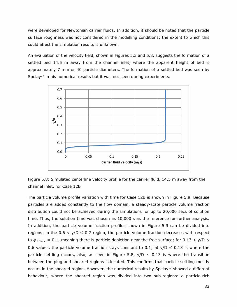
83

were developed for Newtonian carrier fluids. In addition, it should be noted that the particle

surface roughness was not considered in the modelling conditions; the extent to which this

could affect the simulation results is unknown.

An evaluation of the velocity field, shown in Figures 5.3 and 5.8, suggests the formation of a

settled bed 14.5 m away from the channel inlet, where the apparent height of bed is

approximately 7 mm or 40 particle diameters. The formation of a settled bed was seen by

Spelay17 in his numerical results but it was not seen during experiments.

Figure 5.8: Simulated centerline velocity profile for the carrier fluid, 14.5 m away from the

channel inlet, for Case 12B

The particle volume profile variation with time for Case 12B is shown in Figure 5.9. Because

particles are added constantly to the flow domain, a steady-state particle volume fraction

distribution could not be achieved during the simulations for up to 20,000 secs of solution

time. Thus, the solution time was chosen as 10,000 s as the reference for further analysis.

In addition, the particle volume fraction profiles shown in Figure 5.9 can be divided into

regions: in the 0.6 < y/D ≤ 0.7 region, the particle volume fraction decreases with respect

to 𝜙𝑠,𝑏𝑢𝑙𝑘 = 0.1, meaning there is particle depletion near the free surface; for 0.13 < y/D ≤

0.6 values, the particle volume fraction stays constant to 0.1; at y/D ≤ 0.13 is where the

particle settling occurs, also, as seen in Figure 5.8, y/D ~ 0.13 is where the transition

between the plug and sheared regions is located. This confirms that particle settling mostly

occurs in the sheared region. However, the numerical results by Spelay17 showed a different

behaviour, where the sheared region was divided into two sub-regions: a particle-rich

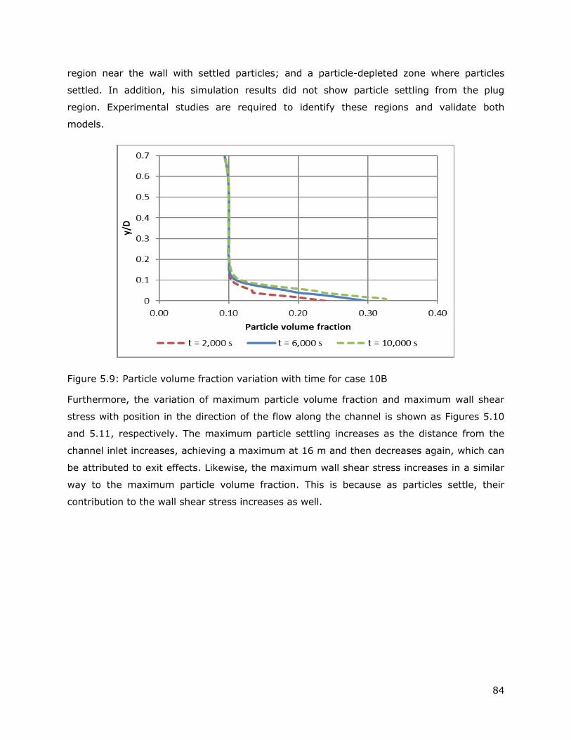
84

region near the wall with settled particles; and a particle-depleted zone where particles

settled. In addition, his simulation results did not show particle settling from the plug

region. Experimental studies are required to identify these regions and validate both

models.

Figure 5.9: Particle volume fraction variation with time for case 10B

Furthermore, the variation of maximum particle volume fraction and maximum wall shear

stress with position in the direction of the flow along the channel is shown as Figures 5.10

and 5.11, respectively. The maximum particle settling increases as the distance from the

channel inlet increases, achieving a maximum at 16 m and then decreases again, which can

be attributed to exit effects. Likewise, the maximum wall shear stress increases in a similar

way to the maximum particle volume fraction. This is because as particles settle, their

contribution to the wall shear stress increases as well.

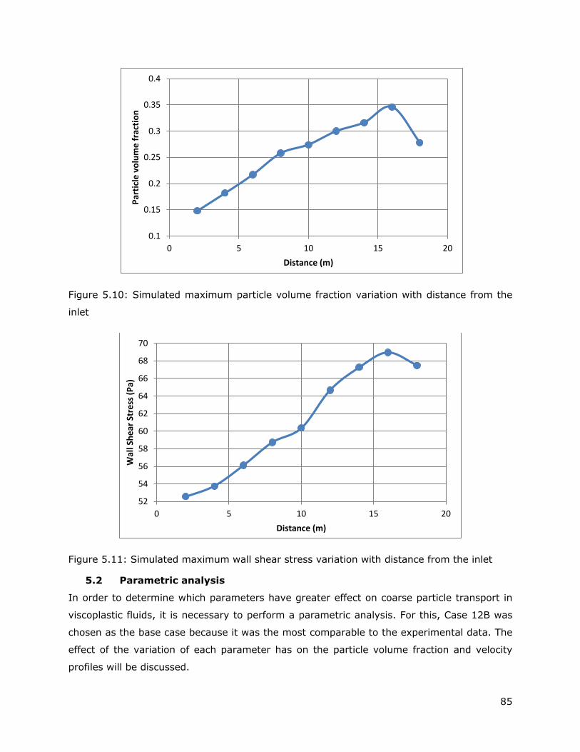
85

Figure 5.10: Simulated maximum particle volume fraction variation with distance from the

inlet

Figure 5.11: Simulated maximum wall shear stress variation with distance from the inlet

5.2 Parametric analysis

In order to determine which parameters have greater effect on coarse particle transport in

viscoplastic fluids, it is necessary to perform a parametric analysis. For this, Case 12B was

chosen as the base case because it was the most comparable to the experimental data. The

effect of the variation of each parameter has on the particle volume fraction and velocity

profiles will be discussed.

0.1

0.15

0.2

0.25

0.3

0.35

0.4

0 5 10 15 20

Par

ticl

e v

olu

me

fra

ctio

n

Distance (m)

52

54

56

58

60

62

64

66

68

70

0 5 10 15 20

Wal

l Sh

ear

Str

ess

(P

a)

Distance (m)

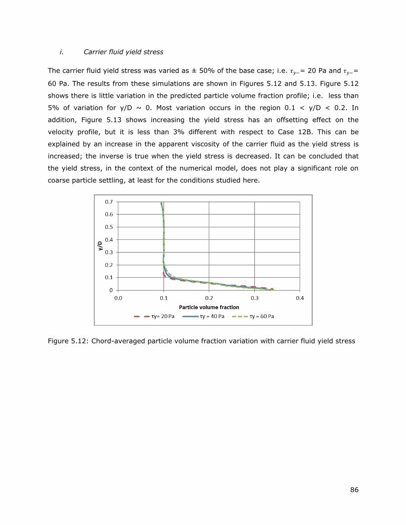
86

i. Carrier fluid yield stress

The carrier fluid yield stress was varied as ± 50% of the base case; i.e. 𝜏𝑦−= 20 Pa and 𝜏𝑦−=

60 Pa. The results from these simulations are shown in Figures 5.12 and 5.13. Figure 5.12

shows there is little variation in the predicted particle volume fraction profile; i.e. less than

5% of variation for y/D ~ 0. Most variation occurs in the region 0.1 < y/D < 0.2. In

addition, Figure 5.13 shows increasing the yield stress has an offsetting effect on the

velocity profile, but it is less than 3% different with respect to Case 12B. This can be

explained by an increase in the apparent viscosity of the carrier fluid as the yield stress is

increased; the inverse is true when the yield stress is decreased. It can be concluded that

the yield stress, in the context of the numerical model, does not play a significant role on

coarse particle settling, at least for the conditions studied here.

Figure 5.12: Chord-averaged particle volume fraction variation with carrier fluid yield stress

87

Figure 5.13: Predicted carrier fluid centerline velocity profile with varying carrier fluid yield

stress

ii. Flow geometry

The impact of changing the channel geometry on particle settling was studied as follows:

Channel diameter and depth of flow (i.e. keeping a constant h/D ratio)

Channel diameter increase with constant depth of flow

Replacement of the semi-circular channel with an equivalent rectangular channel

Channel diameter

Scaling the channel diameter and the depth of flow by 50% has a minor effect on the

normalized particle volume fraction and velocity profiles as shown in Figures 5.14 and 5.15.

However, there is some variation for 0 ≤ y/D ≤ 0.04 where the particle volume fraction at

the wall increases by 16% when compared with the results from Case 12B. In addition, the

height of the settled bed is increased from approximately 7 mm to 14 mm when the channel

diameter is increased by 50%. These results suggest the model could be used for scaling

purposes.

88


and depth of flow


and depth of flow

When the diameter is increased while keeping a constant depth of flow, there is more wall

area for particles to settle. Consequently, particle settling is increased by as much as 17%

with respect to the base case. In addition, the height of the settled bed is increased from 7

mm to 9 mm, approximately. This is shown in Figures 5.16 and 5.17 by plotting the

simulation data against a y/h for an equivalent comparison.

89


and constant depth of flow


and constant depth of flow

Rectangular channel

The channel geometry was changed to a rectangular channel of equivalent hydraulic radius

as the semi-circular channel in Case 12B. Consequently, the dimensions of the rectangular

channel are 0.1077 m in height (equivalent to the depth of flow) and 0.1614 m in width.

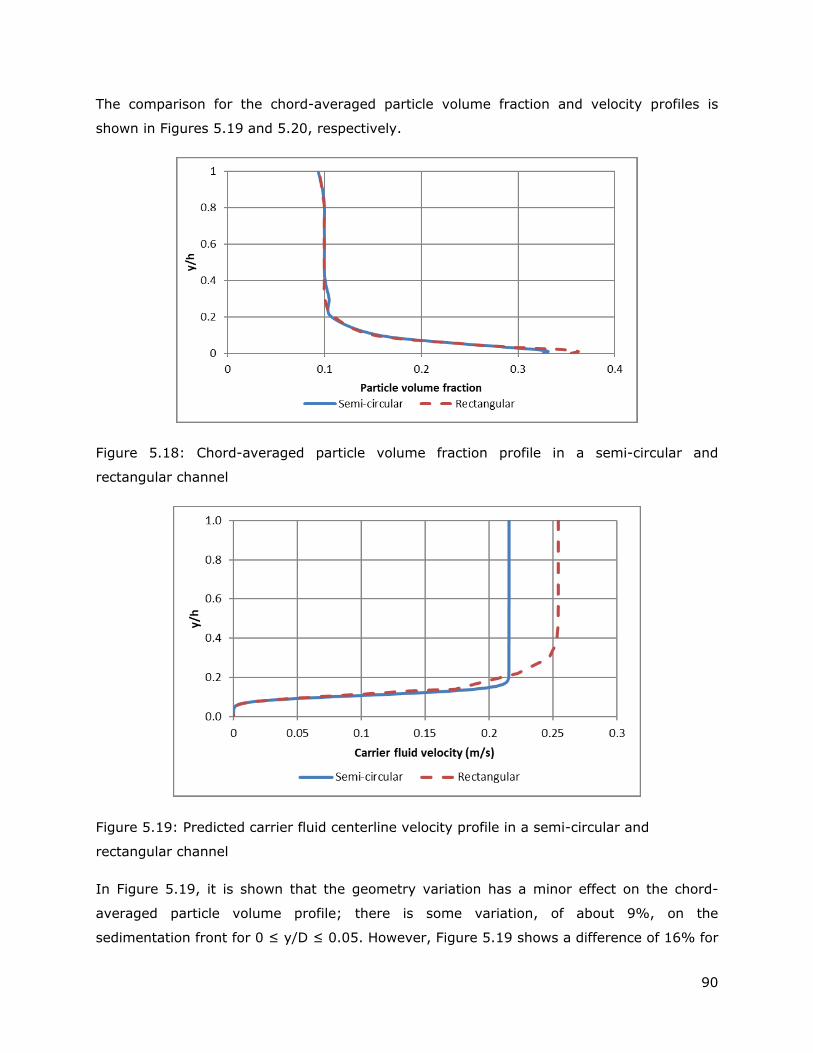
90

The comparison for the chord-averaged particle volume fraction and velocity profiles is

shown in Figures 5.19 and 5.20, respectively.

Figure 5.18: Chord-averaged particle volume fraction profile in a semi-circular and

rectangular channel

Figure 5.19: Predicted carrier fluid centerline velocity profile in a semi-circular and

rectangular channel

In Figure 5.19, it is shown that the geometry variation has a minor effect on the chord-

averaged particle volume profile; there is some variation, of about 9%, on the

sedimentation front for 0 ≤ y/D ≤ 0.05. However, Figure 5.19 shows a difference of 16% for

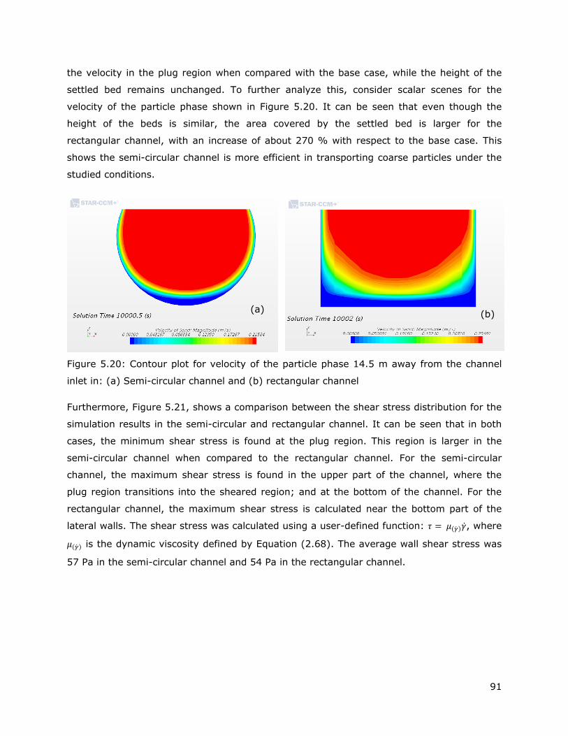
91

the velocity in the plug region when compared with the base case, while the height of the

settled bed remains unchanged. To further analyze this, consider scalar scenes for the

velocity of the particle phase shown in Figure 5.20. It can be seen that even though the

height of the beds is similar, the area covered by the settled bed is larger for the

rectangular channel, with an increase of about 270 % with respect to the base case. This

shows the semi-circular channel is more efficient in transporting coarse particles under the

studied conditions.

Figure 5.20: Contour plot for velocity of the particle phase 14.5 m away from the channel

inlet in: (a) Semi-circular channel and (b) rectangular channel

Furthermore, Figure 5.21, shows a comparison between the shear stress distribution for the

simulation results in the semi-circular and rectangular channel. It can be seen that in both

cases, the minimum shear stress is found at the plug region. This region is larger in the

semi-circular channel when compared to the rectangular channel. For the semi-circular

channel, the maximum shear stress is found in the upper part of the channel, where the

plug region transitions into the sheared region; and at the bottom of the channel. For the

rectangular channel, the maximum shear stress is calculated near the bottom part of the

lateral walls. The shear stress was calculated using a user-defined function: 𝜏 = 𝜇(�̇�)�̇�, where

𝜇(�̇�) is the dynamic viscosity defined by Equation (2.68). The average wall shear stress was

57 Pa in the semi-circular channel and 54 Pa in the rectangular channel.

(a) (b)

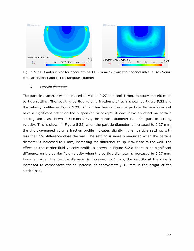
92

Figure 5.21: Contour plot for shear stress 14.5 m away from the channel inlet in: (a) Semi-

circular channel and (b) rectangular channel

iii. Particle diameter

The particle diameter was increased to values 0.27 mm and 1 mm, to study the effect on

particle settling. The resulting particle volume fraction profiles is shown as Figure 5.22 and

the velocity profiles as Figure 5.23. While it has been shown the particle diameter does not

have a significant effect on the suspension viscosity24, it does have an effect on particle

settling since, as shown in Section 2.4.1, the particle diameter is to the particle settling

velocity. This is shown in Figure 5.22, when the particle diameter is increased to 0.27 mm,

the chord-averaged volume fraction profile indicates slightly higher particle settling, with

less than 5% difference close the wall. The settling is more pronounced when the particle

diameter is increased to 1 mm, increasing the difference to up 19% close to the wall. The

effect on the carrier fluid velocity profile is shown in Figure 5.23: there is no significant

difference on the carrier fluid velocity when the particle diameter is increased to 0.27 mm.

However, when the particle diameter is increased to 1 mm, the velocity at the core is

increased to compensate for an increase of approximately 10 mm in the height of the

settled bed.

(a) (b)

93

Figure 5.22: Chord-averaged particle volume fraction with varying particle diameter

Figure 5.23: Predicted carrier fluid centerline velocity profile with varying particle diameter

iv. Bulk particle volume fraction

The bulk particle volume fraction of the suspension was increased to 0.2 and 0.3 v/v. The

resulting particle volume fraction and velocity profiles are shown in Figures 5.24 and 5.26.

94

Figure 5.24: Chord-averaged particle volume fraction with varying particle volume fraction

As expected, increasing the particle volume fraction tends to hinder settling. Figure 5.24

shows the chord-averaged particle volume fraction profiles, for bulk volume fractions of 0.1

and 0.2 v/v the profiles tend to the same values as at y/D approaches zero. In addition, the

deviation from the particle volume fraction at the core is higher for the 0.1 v/v case. To

illustrate this point, the volume fraction profiles are normalized using the average particle

volume fraction, as shown in Figure 5.25. As the bulk particle volume fraction is increased

the deviation from the volume fraction of the plug decreases. The carrier fluid velocity

profiles, shown in Figure 5.26, also show a decrease in size of the settled bed as the inlet

particle volume fraction is increased.

Figure 5.25: Relative particle volume fraction profiles with varying inlet particle volume

fraction

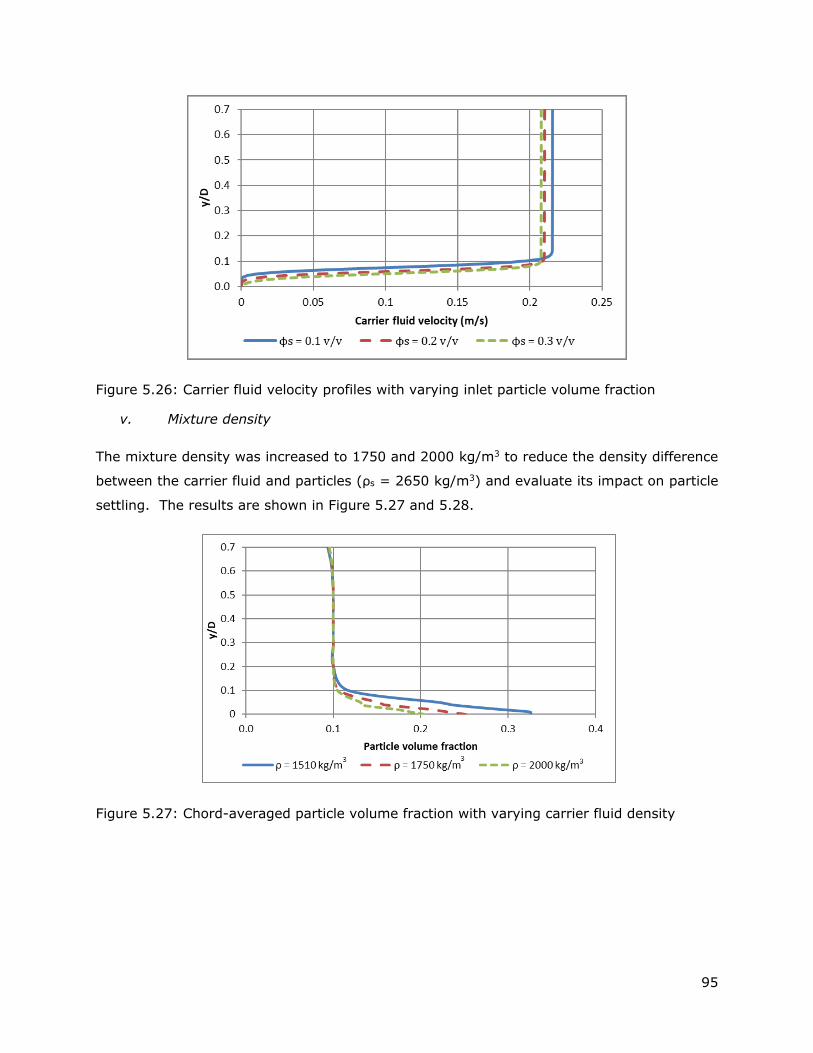
95

Figure 5.26: Carrier fluid velocity profiles with varying inlet particle volume fraction

v. Mixture density

The mixture density was increased to 1750 and 2000 kg/m3 to reduce the density difference

between the carrier fluid and particles (ρs = 2650 kg/m3) and evaluate its impact on particle

settling. The results are shown in Figure 5.27 and 5.28.

Figure 5.27: Chord-averaged particle volume fraction with varying carrier fluid density

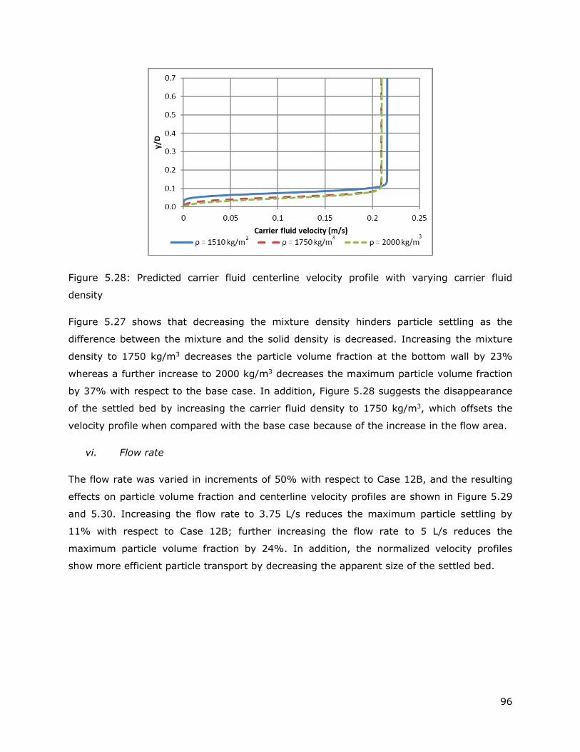
96

Figure 5.28: Predicted carrier fluid centerline velocity profile with varying carrier fluid

density

Figure 5.27 shows that decreasing the mixture density hinders particle settling as the

difference between the mixture and the solid density is decreased. Increasing the mixture

density to 1750 kg/m3 decreases the particle volume fraction at the bottom wall by 23%

whereas a further increase to 2000 kg/m3 decreases the maximum particle volume fraction

by 37% with respect to the base case. In addition, Figure 5.28 suggests the disappearance

of the settled bed by increasing the carrier fluid density to 1750 kg/m3, which offsets the

velocity profile when compared with the base case because of the increase in the flow area.

vi. Flow rate

The flow rate was varied in increments of 50% with respect to Case 12B, and the resulting

effects on particle volume fraction and centerline velocity profiles are shown in Figure 5.29

and 5.30. Increasing the flow rate to 3.75 L/s reduces the maximum particle settling by

11% with respect to Case 12B; further increasing the flow rate to 5 L/s reduces the

maximum particle volume fraction by 24%. In addition, the normalized velocity profiles

show more efficient particle transport by decreasing the apparent size of the settled bed.

97

Figure 5.29: Chord averaged particle volume fraction profile with varying flow rate

Figure 5.30: Normalized centerline velocity profile with varying flow rate

From the parametric analysis, it is shown the carrier fluid density, flow rate, and coarse

particle volume fraction each play a major role in coarse particle settling; increasing one of

these parameters can decrease particle settling significantly. However, the implications of

changing these parameters must be considered to determine the best approach from an

operational point of view. For example, increasing the coarse particle volume fraction might

have effects in the erosion rate of the channel, increasing the carrier fluid density might not

be beneficial for the rest of the process, since this would imply adding more particles to the

system; furthermore, increasing the flow rate of the suspension is dependent on pump

capacity and can affect erosion of the pipe walls. On the other hand, varying the yield stress

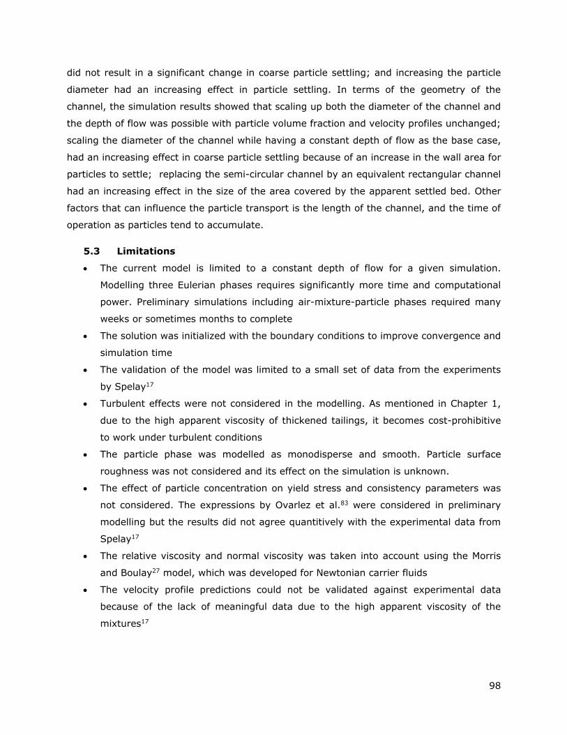
98

did not result in a significant change in coarse particle settling; and increasing the particle

diameter had an increasing effect in particle settling. In terms of the geometry of the

channel, the simulation results showed that scaling up both the diameter of the channel and

the depth of flow was possible with particle volume fraction and velocity profiles unchanged;

scaling the diameter of the channel while having a constant depth of flow as the base case,

had an increasing effect in coarse particle settling because of an increase in the wall area for

particles to settle; replacing the semi-circular channel by an equivalent rectangular channel

had an increasing effect in the size of the area covered by the apparent settled bed. Other

factors that can influence the particle transport is the length of the channel, and the time of

operation as particles tend to accumulate.

5.3 Limitations

The current model is limited to a constant depth of flow for a given simulation.

Modelling three Eulerian phases requires significantly more time and computational

power. Preliminary simulations including air-mixture-particle phases required many

weeks or sometimes months to complete

The solution was initialized with the boundary conditions to improve convergence and

simulation time

The validation of the model was limited to a small set of data from the experiments

by Spelay17

Turbulent effects were not considered in the modelling. As mentioned in Chapter 1,

due to the high apparent viscosity of thickened tailings, it becomes cost-prohibitive

to work under turbulent conditions

The particle phase was modelled as monodisperse and smooth. Particle surface

roughness was not considered and its effect on the simulation is unknown.

The effect of particle concentration on yield stress and consistency parameters was

not considered. The expressions by Ovarlez et al.83 were considered in preliminary

modelling but the results did not agree quantitively with the experimental data from

Spelay17

The relative viscosity and normal viscosity was taken into account using the Morris

and Boulay27 model, which was developed for Newtonian carrier fluids

The velocity profile predictions could not be validated against experimental data

because of the lack of meaningful data due to the high apparent viscosity of the

mixtures17

99

The model does not account for microstructure changes in the mixture because of

shear rate variation, as it was shown recently by Ovarlez et al.83 during their

experimental studies

5.4 Conclusions

A numerical model was developed to predict coarse particle settling in the laminar,

open-channel flow of non-Newtonian suspensions and successfully compared with

experimental data. There was good agreement between the simulation results and

the experiments by Spelay17 for the particle volume fraction distribution

The simulated velocity profiles suggested the formation of a settled bed for the

conditions that were studied

A parametric analysis was performed to identify the major parameters affecting

coarse particle settling. Increasing the yield stress had a minor effect on the

simulated particle volume fraction and velocity profiles

Increasing the channel diameter, while increasing the depth of flow (constant h/D

values) had a minor effect on the particle volume fraction and velocity profiles. The

height of the settled bed was increased with the scale up as well

Increasing the channel diameter, while maintaining the depth of flow constant with

respect of the base case, had an increase on the maximum particle volume fraction

at the bottom of the channel. Consequently, the velocity profile changed to account

for an increase in size of the settled bed, i.e. the velocity at the core increases

Changing the flow geometry to a rectangular channel of equivalent hydraulic radius

to the base had a minor effect on the shape of the particle volume fraction. However,

there was a significant offset of the velocity profile. Closer inspection of the scalar

scenes revealed that the cross-sectional area of the settled bed increased

significantly in the rectangular channel when compared with the semi-circular

channel results. Thus, a semi-circular channel is more efficient transporting coarse

particles under the studied conditions

Increasing the particle diameter had an increasing effect on coarse particle settling

when evaluation the particle volume fraction profiles. The velocity profiles changed

to account for an increase in particle settling

Increasing the bulk particle volume fraction hindered particle settling. The particle

volume fraction profiles were compared using a relative particle volume fraction,

which showed the smaller the bulk volume fraction the more it deviates from the

particle volume fraction at the plug region. Furthermore, the simulated velocity

100

profiles indicated a decrease in the apparent height of the settled bed with increasing

particle volume fraction

Increasing the carrier fluid density also had a hindering effect on coarse particle

settling. Furthermore, the size of the settled bed decreases with increasing mixture

density.

Increasing the flow rate improves the transport of coarse particles, by decreasing the

particle settling at the bottom of the channel. This is also shown in the velocity

profiles where there is no indication of settled bed.

Of the parameters studied, flow rate, carrier fluid density, and particle volume

fraction were the ones which had the most significant impact on coarse particle

settling. Considerations should be taken on how these parameters affect other

integral parts of the process, such as channel erosion, pump capacity, and friction

losses

5.5 Recommendations

The following studies are recommended to improve the modelling of non-Newtonian

suspensions:

Develop experimental techniques to study the presence of a settled bed more

accurately. This will improve the validation of the model

Develop experimental studies to evaluate microstructure changes in water-clay-sand

mixtures as this would improve our understanding in the area and develop models

that can account for this effect properly

Validate the expressions developed by Ovarlez et al.83 to account for the particle

volume fraction effect on yield stress and consistency index using water-clay-sand

mixtures so they can be incorporated in the modelling stage of these suspensions

Study the effect of particle surface roughness on the rheological parameters and flow

characteristics, to evaluate to what extent this difference affects the velocity field in

viscoplastic carrier fluids

Continue developing the CFD model to include air, clay-water mixture, and solid

particle phases as advances in software and hardware become available

Perform experiments where the velocity distribution of clay-water-sand mixtures can

be measured to further validate the model

101

6. Conclusions and recommendations for future work

6.1 Summary and conclusions

The primary goal of this project was to develop a model, using a commercially-available

CFD software, to predict the flow behaviour of non-Newtonian suspensions under laminar,

open-channel flow conditions. This was achieved by first validating STAR-CCM+ modelling

capabilities in less complex cases. First, the ability of the model to predict depth of flow,

wall shear stress, and velocity field of homogeneous, non-Newtonian mixtures was validated

against experimental data17,45, as shown in Chapter 3. In Chapter 4, shear-induced

migration, single-particle settling, and laminar transport of settling slurries were studied

separately and compared with experimental data29,32,35. Lastly, in Chapter 5, the transport

of monodisperse coarse particles suspended in viscoplastic fluids was modelled and

compared against experimental data17. After a thorough validation, it was possible to study

several modelling conditions, that would be otherwise difficult and expensive with

experiments to determine efficient approaches to coarse particle transport using non-

Newtonian fluids.

The main findings of this project are summarized as follows:

The model developed using STAR-CCM+, for the laminar, open-channel flow of non-

Newtonian fluids can successfully predict the depth of flow, wall shear stress, and

velocity field when compared with experimental data from Spelay17. Also, the local

mixture velocity was studied further by using the laminar sheet flow model44, to

address some of the discrepancies observed earlier during the studies, as shown in

Section 3.2. The simulation results were used to calculate the Fanning friction factor

and compare it with an available correlation53 with excellent agreement. The model

presented in Chapter 3 can be used to study the behaviour of these mixtures under a

wide range of conditions.

Shear-induced migration of neutrally-buoyant particles suspended in a Newtonian

fluid, was modelled using the normal viscosity approach in Chapter 4, which was

compared with experimental data by Hampton et al.29. The simulation results showed

migration towards the center of the tube because of gradients in shear rate.

However, the model is not able to predict particle-wall collisions, which caused a

depletion of the particle volume fraction at the walls in the experiments

Single-particle settling through viscoplastic fluids was modelled implementing two

different correlations. The correlation by Shokrollahzadeh35, which uses an

102

“equivalent Newtonian viscosity” to account for the dynamic viscosity of the

viscoplastic fluids proved to be the better of the two, for the evaluated conditions

shown in Section 4.2. While the model is in good agreement with experimental

data35, it suffers from the same limitations as the correlation; i.e., there is significant

scatter of the results with respect of the Newtonian Drag curve as Re* < 50

The laminar pipeline transport of settling was modelled as preliminary studies of

monodisperse coarse particle settling. While the simulation results capture the

overall behaviour of particle settling in Newtonian slurries when compared to the

experimental data of Gillies et al.32, there were some discrepancies in the particle

volume fraction profiles. This was associated with the stability of the solver as the

particle volume fraction reached the maximum packing fraction in the flow domain.

In addition, the velocity profiles showed an asymmetry with respect of the center of

the pipe that is characteristic of particle settling and asymmetric particle

concentration profiles

In Chapter 5, a model was developed to study monodisperse coarse particle settling

in non-Newtonian fluids under laminar, open-channel flow. The simulated volume

fraction profiles were compared successfully with experimental data from Spelay17.

The simulation results showed that particles settle predominantly in the sheared

zone where they form a stationary bed. The maximum particle volume fraction and

maximum wall shear stress were found 16 m away from the channel inlet

A parametric analysis involving the mixture yield stress, channel geometry, particle

diameter, particle volume fraction, mixture density, and flow rate was performed.

The results showed that increasing flow rate, particle volume fraction, and the

density of the suspending fluid are the parameters which have a greater hindering

effect on coarse particle settling. Also, the simulation results showed that the model

can be used for scaling purposes

6.2 Recommendations for future work

The following studies are proposed to improve the model and the knowledge of non-

Newtonian suspensions:

Perform reliable, high-quality measurements of local velocities of viscoplastic fluids

flowing through an open channel. A comparison with additional experimental data,

maintaining ReH < 1000 and using mixtures with a wide range of yield stresses, for

example 2-40 Pa, could help to address some of the discrepancies observed in some

of the modelling results. In addition, if a Pitot tube is used in conjunction with

103

another measurement method, such as ultrasonic velocity profiling (UVP), one could

validate or disprove the assumptions made for the Pitot tube local velocity

measurements for viscoplastic fluids

Study the ability of the Multiphase segregated model, described in Section 2.6.2, to

model the homogeneous, laminar, open-channel flow of non-Newtonian fluids. This

will allow to study the air and mixture phases separately and make it easier for the

user to extract the desired results

Study in more detail the wall effects in particle volume fraction profiles of neutrally

buoyant particle in a tube. Discrete Element Method (DEM) studies can be done to

account for particle-wall collisions, which can aid in the development of more

accurate models in an Eulerian framework

Study the mechanism(s) that govern particle settling in viscoplastic fluids when Re*

< 50, as that is would provide more insight for modelling purposes. For example,

particle-level numerical studies, using DEM or Lattice-Boltzmann, can be performed

to study the drag around a sphere as they settle in a viscoplastic fluid in more detail

Develop experimental protocols to characterize and evaluate microstructure changes

in water-clay-sand mixtures under shear, as it has been shown the microstructure of

viscoplastic suspensions is shear-dependent, while the model assumes a constant

microstructure. Ovarlez et al.83 used a rheo-X-microtomography setup to study the

microstructure of polystyrene particles suspended in a concentrated emulsion, a

similar setup could be used to study sand-clay-water mixtures

Study the effect of particle surface roughness in the rheological parameters and flow

characteristics. This would provide more insight in how surface roughness affects the

flow field as this was not considered in the modelling. Ovarlez et al.89 used nuclear

magnetic resonance (NMR) to measure the local particle volume fraction and local

suspension velocities in a Couette geometry. A similar setup can be used to

characterize neutrally-buoyant suspensions with rough and smooth particles

Continue developing the CFD model to include air, clay-water mixture, and solid

particle phases at the same time in the calculation of the flow behaviour of non-

Newtonian suspensions, as advances in software and hardware become available, as

this was one of the challenges during this study. This can provide with more

applications for the model, such as the prediction of the slope of the deposit once the

thickened tailings have been disposed.

104

References

(1) National Energy Board. 2016 Estimated Production of Canadian Crude Oil and

Equivalent https://www.neb-one.gc.ca/nrg/sttstc/crdlndptrlmprdct/stt/stmtdprdctn-

eng.html (accessed Apr 21, 2017).

(2) Government of Alberta. Alberta Energy Facts

http://www.energy.alberta.ca/oilsands/791.asp (accessed Apr 21, 2017).

(3) Masliyah, J. H.; Czarnecki, J.; Xu, Z. Colloidal Science in Tailings Management. In

Handbook on Theory and Practice of Bitumen Recovery from Athabasca Oil Sands;

Kingsley Knowledge Publishing, 2011; p 392.

(4) Boger, D. V. Rheology and the resource industries. Chem. Eng. Sci. 2009, 64 (22),

4525–4536.

(5) Oil Sands Magazine. MINING FOR BITUMEN

http://www.oilsandsmagazine.com/technical/mining (accessed Jun 23, 2017).

(6) Alberta Energy. About Oil Sands http://www.energy.alberta.ca/OilSands/791.asp

(accessed Jun 23, 2017).

(7) Government of Alberta. Alberta’s Tailings Management Framework

https://www.aer.ca/about-aer/spotlight-on/alberta-tailings-managment-framework

(accessed Aug 27, 2017).

(8) Alberta Energy Regulator. Directive 085 https://www.aer.ca/rules-and-

regulations/directives/directive-085 (accessed Aug 27, 2017).

(9) Canada’s Oil Sands Innovation Alliance. About COSIA http://www.cosia.ca/about-

cosia (accessed Apr 21, 2017).

(10) Canadian Natural Ltd. Horizon Oil Sands Application for tailings management plan

(TMP); 2016.

(11) Shell Canada Energy. Muskeg River Mine Fluid Tailings Management Plan; 2016.

(12) Shell Canada Energy. Jackpine Mine Fluid Tailings Management Plan; 2016.

(13) Imperial Oil Resources Ventures Limited. Kearl Oil Sands Tailings Management Plan;

2016.

105

(14) Suncor Energy. Report on Sustainability 2017

https://sustainability.suncor.com/2017/en/environment/tailings-management.aspx

(accessed Aug 28, 2017).

(15) Syncrude. Tailings Management Plan Application Syncrude Aurora North Mine; 2016.

(16) Sun, R.; Goldszal, A.; Li, C. Optimizing the capture of oil sand fines in sand beach

area. In Proceedings of the International Oil Sands Tailings Conference; Edmonton,

Canada, 2012.

(17) Spelay, R. B. SOLIDS TRANSPORT IN LAMINAR, OPEN CHANNEL FLOW OF NON-

NEWTONIAN SLURRIES, University of Saskatchewan, 2007.

(18) Shook, C. A.; Gillies, R. G.; Sanders, R. S. Pipeline Hydrotransport with Applications

in the Oil Sand Industry; SRC Pipe Flow Technology Centre: Saskatoon, SK, 2002.

(19) Sumner, R. S.; Munkler, J. J.; Carriere, S. M.; Shook, C. A. Rheology of Kaolin

Slurries Containing Large Silica Particles. J. Hydrol. Hydromechanics 2000, 48 (2),

110–124.

(20) Chhabra, R. P.; Richardson, J. F. Non-Newtonian Flow in the Process Industries,

Fundamentals and Engineering Applications, 1st ed.; Butterworth Heinemann: Oxford,

1999.

(21) Tu, J.; Yeoh, G. H.; Liu, C. Computational fluid dynamics: a practical approach, 1st

Editio.; Butterworth Heinemann: Amsterdam, 2008.

(22) Treinen, J. M.; Cooke, R. Energy induced rheology reduction of flocculated slurries. In

Proceedings of the 18th International Conference on Hydrotransport; BHR Group: Rio

de Janeiro, Brazil, 2010; p 487.

(23) Balmforth, N. J.; Frigaard, I. A.; Ovarlez, G. Yielding to Stress: Recent Developments

in Viscoplastic Fluid Mechanics. Annu. Rev. Fluid Mech. 2014, 46 (1), 121–146.

(24) Mewis, J.; Wagner, N. J. Colloidal Suspension Rheology; Varma, A., Ed.; Cambridge

University Press: New York, 2012.

(25) Krieger, I. M.; Dougherty, T. J. A mechanism of non-Newtonian flow in suspensions of

rigid spheres. Trans Soc Rheol 1959, 3, 137.

(26) Krieger, I. M. Rheology of monodisperse latices. Adv Colloid Interface 1972, 3, 111.

106

(27) Morris, J. F.; Boulay, F. Curvilinear flows of noncolloidal suspensions: The role of

normal stresses. J. Rheol. (N. Y. N. Y). 1999, 43 (5), 1213.

(28) Leighton, D.; Acrivos, A. The shear-induced migration of particles in concentrated

suspensions. J. Fluid Mech. 1987, 181, 415–439.

(29) Hampton, R. E.; Mammoli, A. a.; Graham, A. L.; Tetlow, N.; Altobelli, S. a. Migration

of particles undergoing pressure-driven flow in a circular conduit. J. Rheol. (N. Y. N.

Y). 1997, 41 (3), 621.

(30) Phillips, R. J.; Armstrong, R. C.; Brown, R. A.; Graham, A. L.; Abbott, J. R.; Phillips,

R. J.; Armstrong, R. C.; Brown, R. A.; Graham, A. L.; Abbott, J. R. A constitutive

equation for concentrated suspensions that accounts for shear ‐ induced particle

migration A constitutive equation for concentrated for shear-induced particle

migration suspensions that accounts. Phys. Fluids 1992, 30, 30–40.

(31) Richardson, J. F.; Zaki, W. N. Sedimentation and fluidization. Trans. Inst. Chem.

1954, 35, 32.

(32) Gillies, R. G.; Hill, K. B.; McKibben, M. J.; Shook, C. A. Solids transport by laminar

Newtonian flows. Powder Technol. 1999, 104 (3), 269–277.

(33) Treinen, J. M.; Jacobs, J. The Applicability of The Eulerian-Eulerian CFD Approach

Using Granular Kinetic Theory to Predict Particle Settling and Migration in Viscoplastic

Fluids. In 17th International Conference on Transport and Sedimentation of Solid

Particles; Sobota, J., van Rhee, C., Eds.; Wroclaw: Delft, The Netherlands, 2015; pp

345–354.

(34) Sittoni, L.; Talmon, A.; van Kester, J.; Uittenbogaard, R. Latest numerical

developments for the prediction of beaching flow and segregating behavior of thick

Non-Newtonian mixtures. In 17th International Conference on Transport and

Sedimentation of Solid Particles; Sobota, J., van Rhee, C., Eds.; Wroclaw: Delft, The

Netherlands, 2015; pp 309–316.

(35) Shokrollahzadeh, A. Terminal Settling Velocity of a Sphere in a non-Newtonian Fluid,

University of Alberta, 2015.

(36) Straub, L. G.; Silberman, E.; Nelson, H. C. Open channel flow at small Reynolds

numbers. Trans ASCE 1958, 123, 685–706.

107

(37) Chow, V. Te. Open-channel hydraulics; McGraw-Hill: New York, 1959.

(38) White, F. Fluid Mechanics, 8th editio.; McGraw-Hill: New York, 2016.

(39) Haeri, S.; Hashemabadi, S. H. Experimental Study of Gravity-Driven Film Flow of

Non-Newtonian Fluids. Chem. Eng. Commun. 2008, 196 (5), 519–529.

(40) Slatter, P.; Haldenwang, R.; Chhabra, R. P. The Sheet Flow Viscometer. In

Proceedings of the 18th Conference on the Hydraulic Transport of Solids; BHR Group

Ltd: Rio de Janeiro, 2010; pp 299–307.

(41) Astarita, G.; Marrucci, G.; Palumbo, G. Non-Newtonian Gravity Flow Along Inclined

Plane Surfaces. I E Fundam. 1964, 3 (4), 333–339.

(42) Coussot, P.; Proust, S. Slow, unconfined spreading of a mudflow. J. Geophys. Res.

1996, 101 (B11), 25217–25229.

(43) Coussot, P. Steady, laminar, flow of concentrated mud suspensions in open channel.

J. Hydraul. Res. 1994, 32 (4), 535–559.

(44) DE KEE, D.; CHHABRA, R. P.; POWLEY, M. B.; ROY, S. Flow of Viscoplastic Fluids on

an Inclined Plane: Evaluation of Yield Stress. Chem. Eng. Commun. 1990, 96 (1),

229–239.

(45) Haldenwang, R.; Kotzé, R.; Chhabra, R. Determining the viscous behavior of non-

newtonian fluids in a flume using a laminar sheet flow model and Ultrasonic Velocity

Profiling (UVP) system. J. Brazilian Soc. Mech. Sci. Eng. 2012, 34 (3), 276–284.

(46) Alderman, N. J.; Haldenwang, R. A review of Newtonian and non-Newtonian flow in

rectangular open channels. In Proceedings of the 17th International on the Hydraulic

Transport of Solids; BHR Group Ltd: Cape Town, 2007.

(47) Haldenwang, R.; Slatter, P. Experimental procedure and database for non-Newtonian

open channel flow. J. Hydraul. Res. 2006, 44 (2), 283–287.

(48) Kozicki, W.; Tiu, C. Parametric modelling of flow geometries in non-Newtonian flows.

Encyclopedia of Fluid Mechanics; Gulf Publishing Co, 1986; pp 199–252.

(49) Zhang, H.; Ren, Z. Discussion of resistance of hyperconcentrated flow in open

channels. Sci. Sin. (Series A) 1982, 25 (12), 1332–1342.

108

(50) Abulnaga, B. Slurry Systems Handbook; McGraw-Hill: New York, 2002.

(51) Haldenwang, R.; Slatter, P.; Chhabra, R. Laminar and transitional flow in open

channels for non-Newtonian fluids. In Proceedings of the 15th International on the

Hydraulic Transport of Solids; Heywood, N. I., Ed.; BHR Group Ltd: Banff, 2002.

(52) Burger, J.; Haldenwang, R.; Alderman, N. Friction factor-Reynolds number

relationship for laminar flow of non-Newtonian fluids in open channels of different

cross-sectional shapes. Chem. Eng. Sci. 2010, 65 (11), 3549–3556.

(53) Burger, J. H.; Haldenwang, R.; Chhabra, R. P.; Alderman, N. J. Power law and

composite power law friction factor correlations for laminar and turbulent non-

Newtonian open channel flow. J. Brazilian Soc. Mech. Sci. Eng. 2015, 37 (2), 601–

612.

(54) Garcia, F.; Garcia, J.; Padrino, J.; Mata, C.; Trallero, J.; Joseph, D. Power law and

composite power law friction factor correlations for laminar and turbulent gas-liquid

flow in horizontal pipelines. Int. J. Multiph. Flow 2003, 29, 1605–1624.

(55) Stokes, G. G. On the effect of internal friction on fluids on the motion of pendulums.

Trans. Cambidge Philos. Soc. 1851, 9, 48.

(56) Schiller, L.; Naumann, A. Über die grundlegenden Berechnungen der

Schwerkraftaufbereitung. Z. Ver. Deutsch Ing. 1993, 77, 318–320.

(57) Rhodes, M. Introduction to Particle Technology, 2nd editio.; John Wiley & Sons Ltd,

2008.

(58) Renaud, M.; Mauret, E.; Chhabra, R. P. Power-Law Fluid Flow Over a Sphere_Average

Shear Rate and Drag Coefficient.pdf. Can. J. Chem. Eng. 2004, 82 (5), 1066–1070.

(59) Chhabra, R. P.; Richardson, J. F. Non-Newtonian Flow and applied rheology:

engineering applications, 2nd ed.; Butterworth Heinemann: Amsterdam, 2008.

(60) Dhole, S. D.; Chhabra, R. P.; Eswaran, V. Flow of power-law fluids past a sphere at

intermediate reynolds numbers. Ind. Eng. Chem. Res. 2006, 45 (13), 4773–4781.

(61) Chhabra, R. P. Bubbles, drops, and particles in non-Newtonian fluids, 2nd ed.; CRC

Taylor & Francis: Boca Raton, FL, 2007.

(62) Beris, A. N.; Tsamopoulos, J. A.; Armstrong, R. C.; Brown, R. A. Creeping motion of a

109

sphere through a Bingham plastic. J. Fluid Mech. 1985, 158, 219–244.

(63) Tabuteau, H.; Coussot, P.; de Bruyn, J. R. Drag force on a sphere in steady motion

through a yield-stress fluid. J. Rheol. (N. Y. N. Y). 2006, 51 (1), 125–137.

(64) Andres, U. T. Equilibrium and motion of spheres in a viscoplastic liquid. Sov. Phys. -

Dokl. 1961, 5, 753.

(65) Uhlherr, P. H. T. A novel method for measuring yield stress in static fluids. In IVth

Nat. Conf. Rheol.; Adelaide, 1986; p 231.

(66) Schurz, J. The yield stress — an empirical reality. Rheol. Acta 1990, 29, 170.

(67) Ansley, R. W.; Smith, T. N. Motion of spherical particles in a Bingham plastic. AIChE

J. 1967, 13, 1193.

(68) Yoshioka, N.; Adachi, K.; Ishimura, H. On creeping flow of a viscoplastic fluid past a

sphere. Kagaku Kogaku 1971, 10, 1144.

(69) Atapattu, D. D.; Chhabra, R. P.; Uhlherr, P. H. T. Creeping sphere motion in

Herschel–Bulkley fluids: flow field and drag. J. Non-Newton. Fluid Mech. 1995, 59,

245.

(70) Wilson, K. C.; Horsley, R. R.; Kealy, T.; Reizes, J. A.; Horsley, M. Direct prediction of

fall velocities in non-Newtonian materials. Int. J. Miner. Process. 2003, 71 (1–4), 17–

30.

(71) Prandtl, L. Neuere Ergebnisse Turbulenzforschung. Z. Ver. Deutsch Ing. 1933, 77

(5), 105–144.

(72) Colebrook, C. F. Turbulent flow in pipes, with particular reference to the transition

region between the smooth and rough pipe laws. J. Inst. Civ. Eng. 1939, 11, 133–

156.

(73) Wilson, K. C.; Thomas, A. D. A new analysis of the turbulent flow of non-Newtonian

fluids. Can. J. Chem. Eng. 1985, 63, 539–546.

(74) Valentik, L.; Whitmore, R. L. The terminal velocity of spheres in Bingham plastics. Br.

J. Appl. Phys. 1965, 16, 1197.

(75) Tran, Q. K.; Trinh, D. T.; Horsley, R. R.; Reizes, J. A. Drag coefficients and settling

110

velocities of spheres in yield-pseudoplastic slurries. ASME Appl. Mech. Div. 1993,

175, 131.

(76) Rutgers, R. Relative viscosity and concentration. Rheol. Acta 1962, 2, 305.

(77) Einstein, A. Berichtigung zu meiner Arbeit: “Eine neue Bestimmung del

Moleküldimensionen.” Ann Phys. 1911, 34 (2), 591.

(78) Parsi, F.; Gadala-Maria, F. Fore-and-aft asymmetry in a concentrated suspension of

solid spheres. J. Rheol. 1987, 325 (32), 725.

(79) Thomas, D. G. Transport characteristics of suspension: VIII. A note on the viscosity of

Newtonian suspensions of uniform spherical particles. J. Colloid Sci. 1965, 20 (3),

267–277.

(80) Chakrabandhu, K.; Singh, R. K. Rheological properties of coarse food suspensions in

tube flow at high temperatures. J. Food Eng. 2005, 66 (1), 117–128.

(81) Mahaut, F.; Chateau, X.; Coussot, P.; Ovarlez, G. Yield stress and elastic modulus of

suspensions of noncolloidal particles in yield stress fluids. 2008, 52, 287–313.

(82) Chateau, X.; Ovarlez, G.; Trung, K. L. Homogenization approach to the behavior of

suspensions of noncolloidal particles in yield stress fluids. J. Rheol. (N. Y. N. Y).

2008, 52 (2), 489.

(83) Ovarlez, G.; Mahaut, F.; Deboeuf, S.; Lenoir, N.; Hormozi, S.; Chateau, X. Flows of

suspensions of particles in yield stress fluids. J. Rheol. (N. Y. N. Y). 2015, 59 (6),

1449–1486.

(84) Drazer, G.; Koplik, J.; Khusid, B.; Acrivos, A. Deterministic and stochastic behaviour

of non-Brownian spheres in sheared suspensions. J. Fluid Mech. 2002, 460 (2002),

307–335.

(85) Eckstein, E. C.; Bailey, D. G.; Shapiro, A. H. Self-diffusion of particles in shear flow of

a suspension. J. Fluid Mech. 1977, 79, 191.

(86) Rao, R. R.; Mondy, L. A.; Baer, T. A.; Altobelli, S. A.; Stephens, T. S. NMR

measurements and simulations of particle migration in non-newtonian fluids. Chem.

Eng. Commun. 2002, 189 (1), 1–22.

(87) Di Felice, R.; Parodi, E. Wall effects on the sedimentation velocity of suspensions in

111

viscous flow. Am. Inst. Chem. Eng. J. 1996, 42 (4), 927–931.

(88) Baldock, T. E.; Tomkins, M. R.; Nielsen, P.; Hughes, M. G. Settling velocity of

sediments at high concentrations. 2006, 51 (2004), 91–100.

(89) Ovarlez, G.; Bertrand, F.; Coussot, P.; Chateau, X. Shear-induced sedimentation in

yield stress fluids. J. Non-Newton. Fluid Mech. 2012, 177–178, 19–28.

(90) Glowinski, R.; Wachs, A. On the numerical simulation of viscoplastic fluid flow;

Glowinski, R., Xu, J., Eds.; Elsevier: Amsterdam, 2011.

(91) Frigaard, I. A.; Nouar, C. On the usage of viscosity regularisation methods for visco-

plastic fluid flow computation. J. Non-Newton. Fluid Mech. 2005, 127 (1), 1–26.

(92) Brady, J. F.; Bossis, G. Stokesian dynamics. Annu Rev Fluid Mech 1988, 20, 111.

(93) Ladd, A. J. C. Numerical simulations of particulate suspensions via discretized

Boltzmann equation: 2. Numerical results. J. Fluid Mech. 1994, 271, 329.

(94) Martys, N. S. Study of a dissipative particle dynamics based approach for modelling

suspensions. J. Rheol. (N. Y. N. Y). 2005, 49 (2), 401.

(95) Melrose, J. R.; Ball, R. C. The pathological behaviour of sheared hard spheres with

hydrodynamic interactions. Euriphys Lett 1995, 32 (6), 535–540.

(96) Ekambara, Ak.; Sanders, R. S.; Nandakumar, K.; Masliyah, J. H. Hydrodynamic

simulation of horizontal slurry pipeline flow using ANSYS-CFX. Ind. Eng. Chem. Res.

2009, 48 (17), 8159–8171.

(97) Eesa, M.; Barigou, M. CFD investigation of the pipe transport of coarse solids in

laminar power law fluids. Chem. Eng. Sci. 2009, 64 (2), 322–333.

(98) Siemens PLM Software. STAR-CCM+ User guide. 2017.

(99) Spelay, R. B.; Adane, K. F.; Sanders, R. S.; Sumner, R. J.; Gillies, R. G. The effect of

low Reynolds number flows on pitot tube measurements. Flow Meas. Instrum. 2015,

45, 247–254.

(100) Antal, S. P.; Lahey, R. T.; Flaherty, J. E. Analysis of phase distribution in fully

developed laminar bubbly two-phase flow. Int. J. Multiph. Flow 1991, 17 (5), 635–

652.

112

(101) Tomac, I.; Gutierrez, M. Fluid lubrication effects on particle flow and transport in a

channel. Int. J. Multiph. Flow 2014, 65 (October), 143–156.

113

APPENDIX A: SOFTWARE AND HARDWARE TECHNICAL SPECIFICATIONS

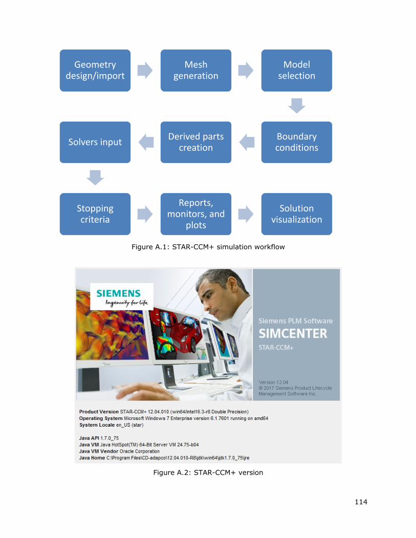
114

Figure A.1: STAR-CCM+ simulation workflow

Figure A.2: STAR-CCM+ version

Geometry design/import

Mesh generation

Model selection

Boundary conditions

Derived parts creation

Solvers input

Stopping criteria

Reports, monitors, and

plots

Solution visualization

115

Table A.1: Computers technical specifications

Computer

name Processor

Number of

cores

Installed

memory (RAM)

Operating

system

BULLDOZER Intel® CoreTM i5-2500

CPU @ 3.30 GHz 4 12.0 GB

Windows 7

Enterprise

CME593617 Intel® CoreTM i7-860

CPU @ 2.80 GHz 8 8.0 GB

Windows 7

Professional

116

APPENDIX B: SIMULATION DATA

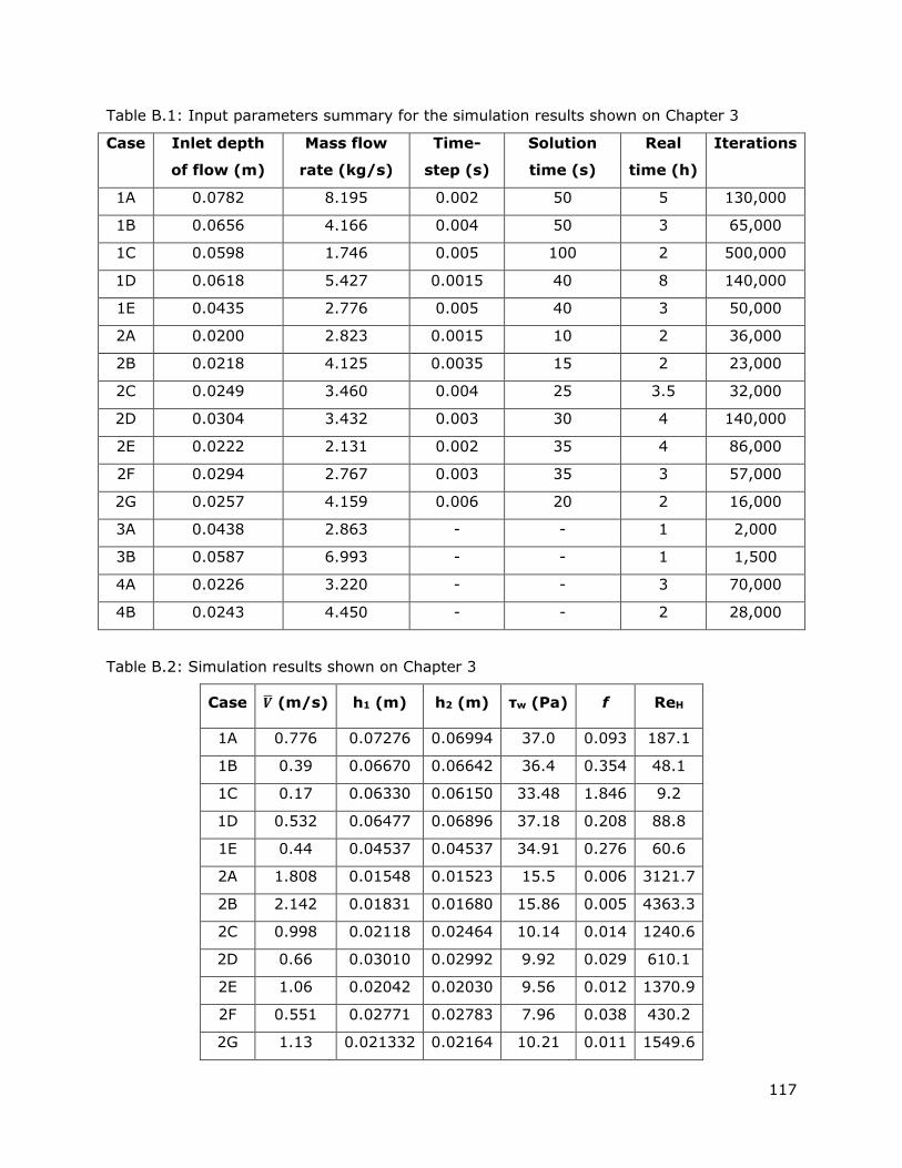
117

Table B.1: Input parameters summary for the simulation results shown on Chapter 3

Case Inlet depth

of flow (m)

Mass flow

rate (kg/s)

Time-

step (s)

Solution

time (s)

Real

time (h)

Iterations

1A 0.0782 8.195 0.002 50 5 130,000

1B 0.0656 4.166 0.004 50 3 65,000

1C 0.0598 1.746 0.005 100 2 500,000

1D 0.0618 5.427 0.0015 40 8 140,000

1E 0.0435 2.776 0.005 40 3 50,000

2A 0.0200 2.823 0.0015 10 2 36,000

2B 0.0218 4.125 0.0035 15 2 23,000

2C 0.0249 3.460 0.004 25 3.5 32,000

2D 0.0304 3.432 0.003 30 4 140,000

2E 0.0222 2.131 0.002 35 4 86,000

2F 0.0294 2.767 0.003 35 3 57,000

2G 0.0257 4.159 0.006 20 2 16,000

3A 0.0438 2.863 - - 1 2,000

3B 0.0587 6.993 - - 1 1,500

4A 0.0226 3.220 - - 3 70,000

4B 0.0243 4.450 - - 2 28,000

Table B.2: Simulation results shown on Chapter 3

Case �̅� (m/s) h1 (m) h2 (m) τw (Pa) f ReH

1A 0.776 0.07276 0.06994 37.0 0.093 187.1

1B 0.39 0.06670 0.06642 36.4 0.354 48.1

1C 0.17 0.06330 0.06150 33.48 1.846 9.2

1D 0.532 0.06477 0.06896 37.18 0.208 88.8

1E 0.44 0.04537 0.04537 34.91 0.276 60.6

2A 1.808 0.01548 0.01523 15.5 0.006 3121.7

2B 2.142 0.01831 0.01680 15.86 0.005 4363.3

2C 0.998 0.02118 0.02464 10.14 0.014 1240.6

2D 0.66 0.03010 0.02992 9.92 0.029 610.1

2E 1.06 0.02042 0.02030 9.56 0.012 1370.9

2F 0.551 0.02771 0.02783 7.96 0.038 430.2

2G 1.13 0.021332 0.02164 10.21 0.011 1549.6

118

Table B.3: Simplified simulation results for the centerline velocity profiles for cases 2A, 2B,

and 2G

Case 2A Case 2B Case 2G

y/h v/V y/h v/V y/h v/V

1.0 1.65 1.0 1.53 1.0 1.43

0.9 1.65 0.9 1.53 0.9 1.43

0.8 1.65 0.8 1.53 0.8 1.43

0.7 1.64 0.7 1.53 0.7 1.43

0.6 1.63 0.6 1.52 0.6 1.42

0.5 1.60 0.5 1.52 0.5 1.42

0.4 1.51 0.4 1.50 0.4 1.39

0.3 1.33 0.3 1.41 0.3 1.30

0.2 1.03 0.2 1.14 0.2 1.06

0.1 0.57 0.1 0.65 0.1 0.63

0.05 0.33 0.05 0.38 0.05 0.34

0 0 0 0 0 0


4A, and 4B

Case 3A Case 3B Case 4A Case 4B

y/h v/V y/h v/V y/h v/V y/h v/V

1.0 1.41 1.0 1.40 1.0 1.16 1.0 1.16

0.9 1.40 0.9 1.40 0.9 1.16 0.9 1.16

0.8 1.38 0.8 1.37 0.8 1.16 0.8 1.16

0.7 1.33 0.7 1.33 0.7 1.16 0.7 1.16

0.6 1.25 0.6 1.25 0.6 1.15 0.6 1.16

0.5 1.15 0.5 1.15 0.5 1.10 0.5 1.15

0.4 1.00 0.4 1.01 0.4 1.10 0.4 1.13

0.3 0.82 0.3 0.82 0.3 1.04 0.3 1.04

0.2 0.60 0.2 0.6 0.2 0.88 0.2 0.87

0.1 0.34 0.1 0.32 0.1 0.57 0.1 0.55

0.05 0.17 0.05 0.17 0.05 0.32 0.05 0.30

0 0 0 0 0 0 0 0

119


Case Time-step (s) Solution time (s) Real time (h) Iterations

5A 0.0001 – 1.8 1000 1 7500

5B 0.0001 – 1.0 1000 0.5 10500

5C 0.0001 – 0.8 4000 4 26000

6 0.0005 0.75 < 0.5 26000

7 0.0005 0.5 < 0.5 18000

8 0.0005 0.5 < 0.5 20000

9 0.0005 1.0 < 0.5 50000

10A 0.0005 0.5 < 0.5 20000

10B 0.0005 0.75 < 0.5 30000

11A 0.001 – 0.3 2200 2 40000

11B 0.001 – 0.1 1200 1.5 21000

Table B.6: Simplified simulation results for volume fraction profiles for cases 5A, 5B, and 5C

Case 5A Case 5B Case 5C

r/R 𝝓𝒔 r/R 𝝓𝒔 r/R 𝝓𝒔

1.0 0.141 1.0 0.220 1.0 0.382

0.9 0.148 0.9 0.230 0.9 0.396

0.8 0.157 0.8 0.244 0.8 0.413

0.7 0.167 0.7 0.257 0.7 0.431

0.6 0.179 0.6 0.274 0.6 0.450

0.5 0.194 0.5 0.294 0.5 0.471

0.4 0.213 0.4 0.318 0.4 0.498

0.3 0.238 0.3 0.355 0.3 0.522

0.2 0.277 0.2 0.416 0.2 0.557

0.1 0.334 0.1 0.488 0.1 0.581

0.05 0.357 0.05 0.508 0.05 0.588

0 0.357 0 0.521 0 0.589

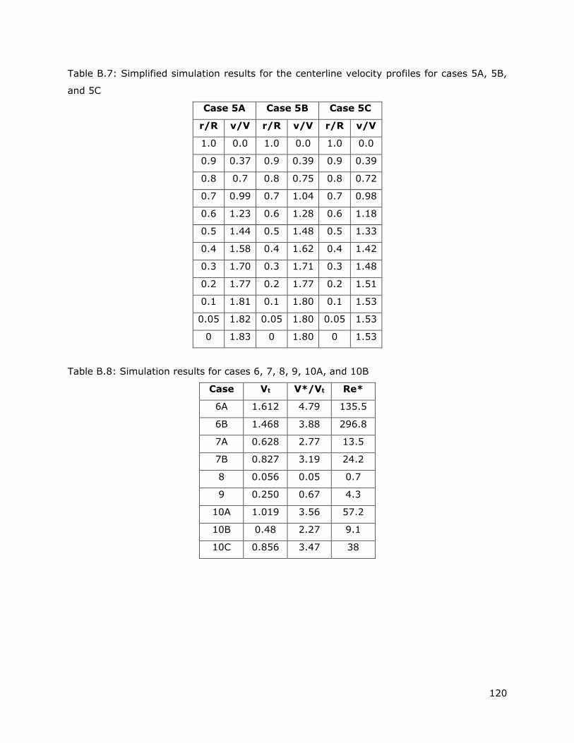
120


and 5C

Case 5A Case 5B Case 5C

r/R v/V r/R v/V r/R v/V

1.0 0.0 1.0 0.0 1.0 0.0

0.9 0.37 0.9 0.39 0.9 0.39

0.8 0.7 0.8 0.75 0.8 0.72

0.7 0.99 0.7 1.04 0.7 0.98

0.6 1.23 0.6 1.28 0.6 1.18

0.5 1.44 0.5 1.48 0.5 1.33

0.4 1.58 0.4 1.62 0.4 1.42

0.3 1.70 0.3 1.71 0.3 1.48

0.2 1.77 0.2 1.77 0.2 1.51

0.1 1.81 0.1 1.80 0.1 1.53

0.05 1.82 0.05 1.80 0.05 1.53

0 1.83 0 1.80 0 1.53

Table B.8: Simulation results for cases 6, 7, 8, 9, 10A, and 10B

Case Vt V*/Vt Re*

6A 1.612 4.79 135.5

6B 1.468 3.88 296.8

7A 0.628 2.77 13.5

7B 0.827 3.19 24.2

8 0.056 0.05 0.7

9 0.250 0.67 4.3

10A 1.019 3.56 57.2

10B 0.48 2.27 9.1

10C 0.856 3.47 38

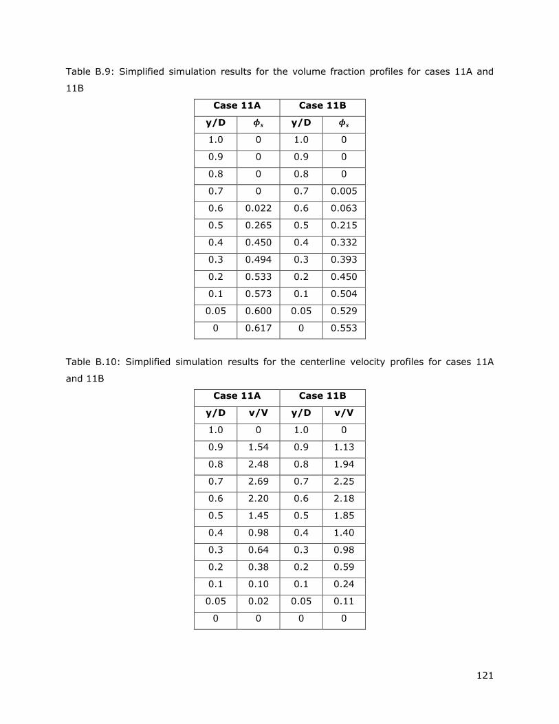
121

Table B.9: Simplified simulation results for the volume fraction profiles for cases 11A and

11B

Case 11A Case 11B

y/D 𝝓𝒔 y/D 𝝓𝒔

1.0 0 1.0 0

0.9 0 0.9 0

0.8 0 0.8 0

0.7 0 0.7 0.005

0.6 0.022 0.6 0.063

0.5 0.265 0.5 0.215

0.4 0.450 0.4 0.332

0.3 0.494 0.3 0.393

0.2 0.533 0.2 0.450

0.1 0.573 0.1 0.504

0.05 0.600 0.05 0.529

0 0.617 0 0.553

Table B.10: Simplified simulation results for the centerline velocity profiles for cases 11A

and 11B

Case 11A Case 11B

y/D v/V y/D v/V

1.0 0 1.0 0

0.9 1.54 0.9 1.13

0.8 2.48 0.8 1.94

0.7 2.69 0.7 2.25

0.6 2.20 0.6 2.18

0.5 1.45 0.5 1.85

0.4 0.98 0.4 1.40

0.3 0.64 0.3 0.98

0.2 0.38 0.2 0.59

0.1 0.10 0.1 0.24

0.05 0.02 0.05 0.11

0 0 0 0

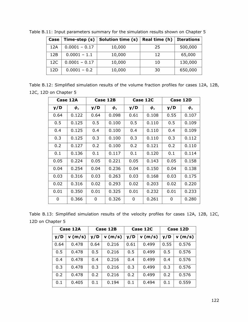
122


Case Time-step (s) Solution time (s) Real time (h) Iterations

12A 0.0001 – 0.17 10,000 25 500,000

12B 0.0001 – 1.1 10,000 12 65,000

12C 0.0001 – 0.17 10,000 10 130,000

12D 0.0001 – 0.2 10,000 30 650,000

Table B.12: Simplified simulation results of the volume fraction profiles for cases 12A, 12B,

12C, 12D on Chapter 5

Case 12A Case 12B Case 12C Case 12D

y/D 𝝓𝒔 y/D 𝝓𝒔 y/D 𝝓𝒔 y/D 𝝓𝒔

0.64 0.122 0.64 0.098 0.61 0.108 0.55 0.107

0.5 0.125 0.5 0.100 0.5 0.110 0.5 0.109

0.4 0.125 0.4 0.100 0.4 0.110 0.4 0.109

0.3 0.125 0.3 0.100 0.3 0.110 0.3 0.112

0.2 0.127 0.2 0.100 0.2 0.121 0.2 0.110

0.1 0.136 0.1 0.117 0.1 0.120 0.1 0.114

0.05 0.224 0.05 0.221 0.05 0.143 0.05 0.158

0.04 0.254 0.04 0.236 0.04 0.150 0.04 0.138

0.03 0.316 0.03 0.263 0.03 0.168 0.03 0.175

0.02 0.316 0.02 0.293 0.02 0.203 0.02 0.220

0.01 0.350 0.01 0.325 0.01 0.232 0.01 0.233

0 0.366 0 0.326 0 0.261 0 0.280

Table B.13: Simplified simulation results of the velocity profiles for cases 12A, 12B, 12C,

12D on Chapter 5


y/D v (m/s) y/D v (m/s) y/D v (m/s) y/D v (m/s)

0.64 0.478 0.64 0.216 0.61 0.499 0.55 0.576

0.5 0.478 0.5 0.216 0.5 0.499 0.5 0.576

0.4 0.478 0.4 0.216 0.4 0.499 0.4 0.576

0.3 0.478 0.3 0.216 0.3 0.499 0.3 0.576

0.2 0.478 0.2 0.216 0.2 0.499 0.2 0.576

0.1 0.405 0.1 0.194 0.1 0.494 0.1 0.559

123

Table B.13: Simplified simulation results of the velocity profiles for cases 12A, 12B, 12C,

12D on Chapter 5 (continued)


y/D v (m/s) y/D v (m/s) y/D v (m/s) y/D v (m/s)

0.05 0.006 0.05 0.012 0.05 0.227 0.05 0.245

0.04 0.001 0.04 0.003 0.04 0.115 0.04 0.140

0.03 0.000 0.03 0.000 0.03 0.032 0.03 0.063

0.02 0.000 0.02 0.000 0.02 0.003 0.02 0.019

0.01 0.000 0.01 0.000 0.01 0.000 0.01 0.004

0 0.000 0 0.000 0 0.000 0 0

Table B.14: Simplified simulation results of the volume fraction profiles for case 12B varying

solution time

t = 2000s t = 4000s t = 6000s t = 8000s t = 10000 s

y/D 𝝓𝒔 y/D 𝝓𝒔 y/D 𝝓𝒔 y/D 𝝓𝒔 y/D 𝝓𝒔

0.7 0.094 0.7 0.094 0.7 0.094 0.7 0.094 0.7 0.094

0.62 0.098 0.62 0.098 0.62 0.098 0.62 0.098 0.62 0.098

0.51 0.100 0.51 0.100 0.51 0.100 0.51 0.100 0.51 0.100

0.4 0.100 0.4 0.100 0.4 0.100 0.4 0.100 0.4 0.100

0.3 0.100 0.3 0.100 0.3 0.100 0.3 0.100 0.3 0.100

0.2 0.100 0.2 0.100 0.2 0.100 0.2 0.100 0.2 0.100

0.1 0.100 0.1 0.105 0.1 0.110 0.1 0.114 0.1 0.117

0.05 0.133 0.05 0.158 0.05 0.184 0.05 0.205 0.05 0.221

0.04 0.134 0.04 0.169 0.04 0.199 0.04 0.220 0.04 0.236

0.03 0.160 0.03 0.200 0.03 0.229 0.03 0.248 0.03 0.263

0.02 0.192 0.02 0.228 0.02 0.254 0.02 0.274 0.02 0.293

0.01 0.216 0.01 0.251 0.01 0.276 0.01 0.302 0.01 0.325

0 0.239 0 0.274 0 0.298 0 0.294 0 0.326

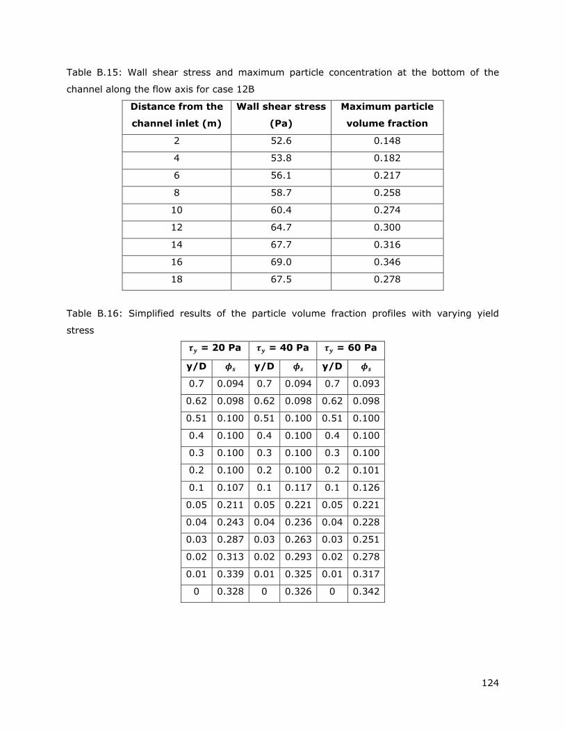
124

Table B.15: Wall shear stress and maximum particle concentration at the bottom of the

channel along the flow axis for case 12B

Distance from the

channel inlet (m)

Wall shear stress

(Pa)

Maximum particle

volume fraction

2 52.6 0.148

4 53.8 0.182

6 56.1 0.217

8 58.7 0.258

10 60.4 0.274

12 64.7 0.300

14 67.7 0.316

16 69.0 0.346

18 67.5 0.278

Table B.16: Simplified results of the particle volume fraction profiles with varying yield

stress

𝝉𝒚 = 20 Pa 𝝉𝒚 = 40 Pa 𝝉𝒚 = 60 Pa

y/D 𝝓𝒔 y/D 𝝓𝒔 y/D 𝝓𝒔

0.7 0.094 0.7 0.094 0.7 0.093

0.62 0.098 0.62 0.098 0.62 0.098

0.51 0.100 0.51 0.100 0.51 0.100

0.4 0.100 0.4 0.100 0.4 0.100

0.3 0.100 0.3 0.100 0.3 0.100

0.2 0.100 0.2 0.100 0.2 0.101

0.1 0.107 0.1 0.117 0.1 0.126

0.05 0.211 0.05 0.221 0.05 0.221

0.04 0.243 0.04 0.236 0.04 0.228

0.03 0.287 0.03 0.263 0.03 0.251

0.02 0.313 0.02 0.293 0.02 0.278

0.01 0.339 0.01 0.325 0.01 0.317

0 0.328 0 0.326 0 0.342

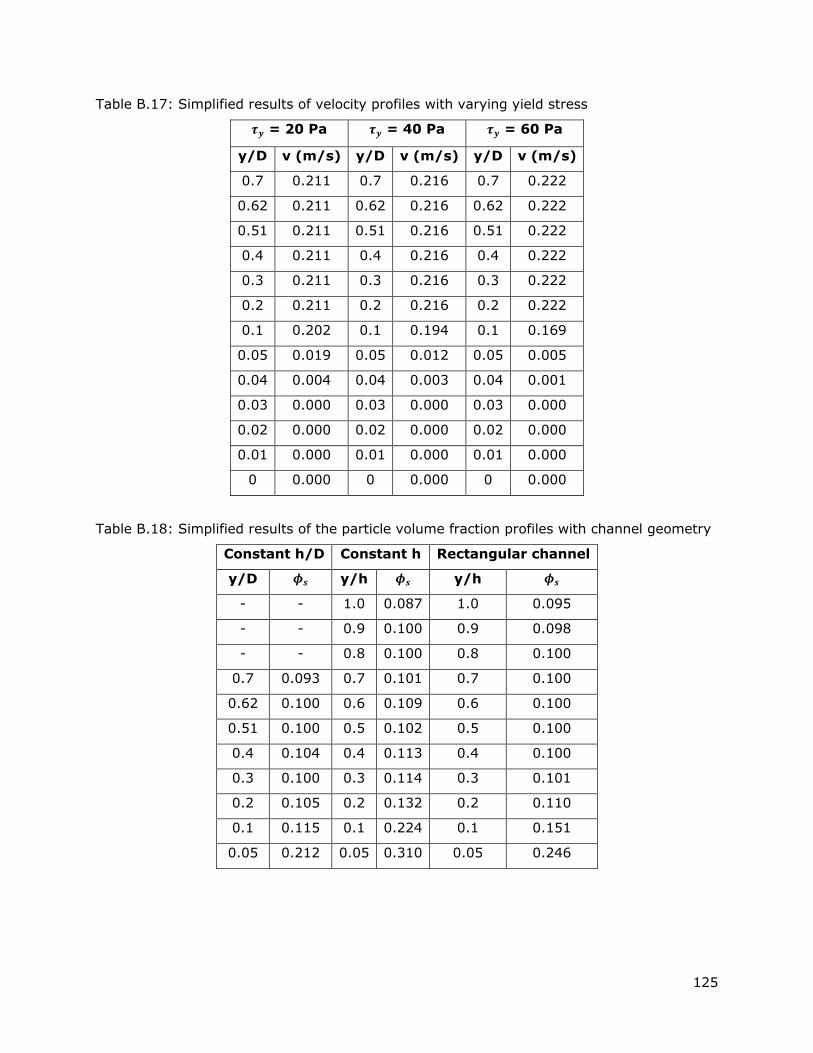
125

Table B.17: Simplified results of velocity profiles with varying yield stress

𝝉𝒚 = 20 Pa 𝝉𝒚 = 40 Pa 𝝉𝒚 = 60 Pa

y/D v (m/s) y/D v (m/s) y/D v (m/s)

0.7 0.211 0.7 0.216 0.7 0.222

0.62 0.211 0.62 0.216 0.62 0.222

0.51 0.211 0.51 0.216 0.51 0.222

0.4 0.211 0.4 0.216 0.4 0.222

0.3 0.211 0.3 0.216 0.3 0.222

0.2 0.211 0.2 0.216 0.2 0.222

0.1 0.202 0.1 0.194 0.1 0.169

0.05 0.019 0.05 0.012 0.05 0.005

0.04 0.004 0.04 0.003 0.04 0.001

0.03 0.000 0.03 0.000 0.03 0.000

0.02 0.000 0.02 0.000 0.02 0.000

0.01 0.000 0.01 0.000 0.01 0.000

0 0.000 0 0.000 0 0.000

Table B.18: Simplified results of the particle volume fraction profiles with channel geometry

Constant h/D Constant h Rectangular channel

y/D 𝝓𝒔 y/h 𝝓𝒔 y/h 𝝓𝒔

- - 1.0 0.087 1.0 0.095

- - 0.9 0.100 0.9 0.098

- - 0.8 0.100 0.8 0.100

0.7 0.093 0.7 0.101 0.7 0.100

0.62 0.100 0.6 0.109 0.6 0.100

0.51 0.100 0.5 0.102 0.5 0.100

0.4 0.104 0.4 0.113 0.4 0.100

0.3 0.100 0.3 0.114 0.3 0.101

0.2 0.105 0.2 0.132 0.2 0.110

0.1 0.115 0.1 0.224 0.1 0.151

0.05 0.212 0.05 0.310 0.05 0.246

126

Table B.18: Simplified results of the particle volume fraction profiles with channel geometry

(continued)


y/D 𝝓𝒔 y/h 𝝓𝒔 y/h 𝝓𝒔

0.04 0.243 0.04 0.332 0.04 0.271

0.03 0.281 0.03 0.357 0.03 0.306

0.02 0.335 0.02 0.388 0.02 0.345

0.01 0.378 0.01 0.385 0.01 0.362

0 0.375 0 0.382 0 0.355

Table B.19: Simplified results of the velocity profiles with channel geometry


y/D v (m/s) y/h v (m/s) y/h v (m/s)

- - 1.0 0.231 1.0 0.254

- - 0.9 0.231 0.9 0.254

- - 0.8 0.231 0.8 0.254

0.7 0.217 0.7 0.231 0.7 0.254

0.62 0.217 0.6 0.231 0.6 0.254

0.51 0.217 0.5 0.231 0.5 0.254

0.4 0.217 0.4 0.229 0.4 0.253

0.3 0.217 0.3 0.221 0.3 0.247

0.2 0.217 0.2 0.200 0.2 0.210

0.1 0.198 0.1 0.018 0.1 0.065

0.05 0.015 0.05 0.000 0.05 0.001

0.04 0.003 0.04 0.000 0.04 0.000

0.03 0.000 0.03 0.000 0.03 0.000

0.02 0.000 0.02 0.000 0.02 0.000

0.01 0.000 0.01 0.000 0.01 0.000

0 0.000 0 0.000 0 0.000

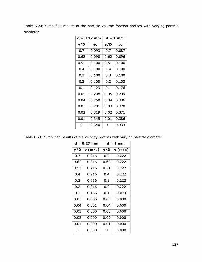
127

Table B.20: Simplified results of the particle volume fraction profiles with varying particle

diameter

d = 0.27 mm d = 1 mm


0.7 0.093 0.7 0.087

0.62 0.098 0.62 0.096

0.51 0.100 0.51 0.100

0.4 0.100 0.4 0.100

0.3 0.100 0.3 0.100

0.2 0.100 0.2 0.102

0.1 0.123 0.1 0.176

0.05 0.238 0.05 0.299

0.04 0.250 0.04 0.336

0.03 0.281 0.03 0.370

0.02 0.319 0.02 0.371

0.01 0.345 0.01 0.386

0 0.340 0 0.333

Table B.21: Simplified results of the velocity profiles with varying particle diameter

d = 0.27 mm d = 1 mm

y/D v (m/s) y/D v (m/s)

0.7 0.216 0.7 0.222

0.62 0.216 0.62 0.222

0.51 0.216 0.51 0.222

0.4 0.216 0.4 0.222

0.3 0.216 0.3 0.222

0.2 0.216 0.2 0.222

0.1 0.186 0.1 0.073

0.05 0.006 0.05 0.000

0.04 0.001 0.04 0.000

0.03 0.000 0.03 0.000

0.02 0.000 0.02 0.000

0.01 0.000 0.01 0.000

0 0.000 0 0.000

128


bulk volume fraction

𝝓𝒔,𝒃𝒖𝒍𝒌 = 𝟎. 𝟐 𝝓𝒔,𝒃𝒖𝒍𝒌 = 𝟎. 𝟑


0.7 0.191 0.7 0.291

0.62 0.197 0.62 0.297

0.51 0.200 0.51 0.300

0.4 0.200 0.4 0.300

0.3 0.200 0.3 0.300

0.2 0.200 0.2 0.301

0.1 0.212 0.1 0.307

0.05 0.271 0.05 0.338

0.04 0.278 0.04 0.341

0.03 0.296 0.03 0.352

0.02 0.314 0.02 0.362

0.01 0.324 0.01 0.368

0 0.335 0 0.376

Table B.23: Simplified results of the velocity profiles with varying particle bulk volume

fraction

𝝓𝒔,𝒃𝒖𝒍𝒌 = 𝟎. 𝟐 𝝓𝒔,𝒃𝒖𝒍𝒌 = 𝟎. 𝟑


0.62 0.210 0.62 0.208

0.51 0.210 0.51 0.208

0.4 0.210 0.4 0.208

0.3 0.210 0.3 0.208

0.2 0.210 0.2 0.208

0.1 0.209 0.1 0.207

0.05 0.056 0.05 0.097

0.04 0.022 0.04 0.053

0.03 0.006 0.03 0.024

0.02 0.001 0.02 0.009

0.01 0.000 0.01 0.003

0 0.000 0 0.000

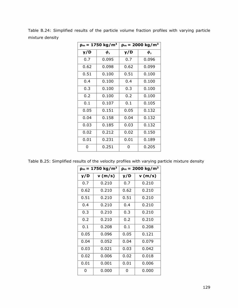
129


mixture density

ρm = 1750 kg/m3 ρm = 2000 kg/m3


0.7 0.095 0.7 0.096

0.62 0.098 0.62 0.099

0.51 0.100 0.51 0.100

0.4 0.100 0.4 0.100

0.3 0.100 0.3 0.100

0.2 0.100 0.2 0.100

0.1 0.107 0.1 0.105

0.05 0.151 0.05 0.132

0.04 0.158 0.04 0.132

0.03 0.185 0.03 0.132

0.02 0.212 0.02 0.150

0.01 0.231 0.01 0.189

0 0.251 0 0.205

Table B.25: Simplified results of the velocity profiles with varying particle mixture density

ρm = 1750 kg/m3 ρm = 2000 kg/m3


0.7 0.210 0.7 0.210

0.62 0.210 0.62 0.210

0.51 0.210 0.51 0.210

0.4 0.210 0.4 0.210

0.3 0.210 0.3 0.210

0.2 0.210 0.2 0.210

0.1 0.208 0.1 0.208

0.05 0.096 0.05 0.121

0.04 0.052 0.04 0.079

0.03 0.021 0.03 0.042

0.02 0.006 0.02 0.018

0.01 0.001 0.01 0.006

0 0.000 0 0.000

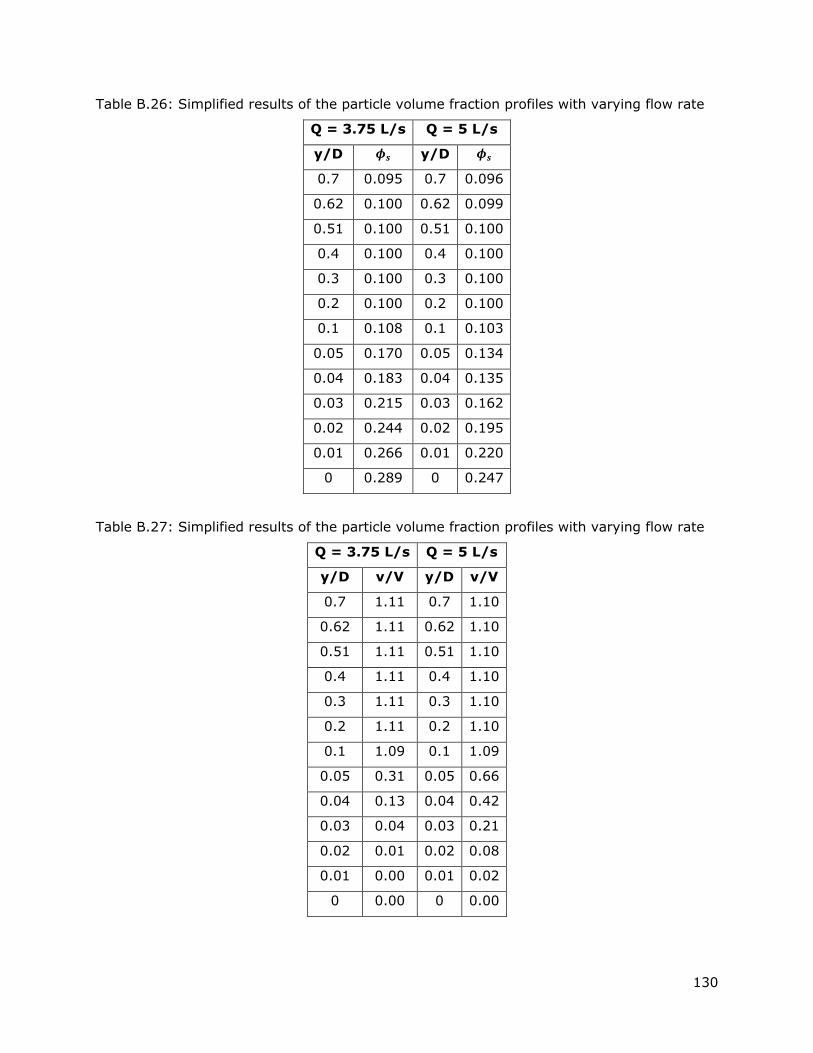
130

Table B.26: Simplified results of the particle volume fraction profiles with varying flow rate

Q = 3.75 L/s Q = 5 L/s


0.7 0.095 0.7 0.096

0.62 0.100 0.62 0.099

0.51 0.100 0.51 0.100

0.4 0.100 0.4 0.100

0.3 0.100 0.3 0.100

0.2 0.100 0.2 0.100

0.1 0.108 0.1 0.103

0.05 0.170 0.05 0.134

0.04 0.183 0.04 0.135

0.03 0.215 0.03 0.162

0.02 0.244 0.02 0.195

0.01 0.266 0.01 0.220

0 0.289 0 0.247

Table B.27: Simplified results of the particle volume fraction profiles with varying flow rate

Q = 3.75 L/s Q = 5 L/s

y/D v/V y/D v/V

0.7 1.11 0.7 1.10

0.62 1.11 0.62 1.10

0.51 1.11 0.51 1.10

0.4 1.11 0.4 1.10

0.3 1.11 0.3 1.10

0.2 1.11 0.2 1.10

0.1 1.09 0.1 1.09

0.05 0.31 0.05 0.66

0.04 0.13 0.04 0.42

0.03 0.04 0.03 0.21

0.02 0.01 0.02 0.08

0.01 0.00 0.01 0.02

0 0.00 0 0.00

CFD Modelling of Laminar, Open-Channel Flows of Non ... · CFD Modelling of Laminar, Open-Channel...

Documents

Transcript of CFD Modelling of Laminar, Open-Channel Flows of Non ... · CFD Modelling of Laminar, Open-Channel...