CFD Modelling of an Underground Water Tank Heat StorageSystem

M. Mahdi Salehi1, W. Kendal Bushe1, Paul Marmion2 and Ray Pradinuk2

1Mechanical Engineering Department, University of British Columbia, Vancouver, BC2Stantec Consulting, Vancouver, BC

Abstract

In this work, CFD is used to simulate the flow in an existing thermallabyrinth located at the basement of a hospital building. This labyrinthis an underground channel equipped with water tanks to increase thethermal mass and reduce the heating and cooling demand of the build-ing. Thermal energy storage in the water tanks is a complex heat trans-fer phenomena involving turbulent forced convection, solid conduc-tion and natural convection. The turbulent forced convection happensbetween the water tank outside surface and the air flow through thelabyrinth. The heat is then conducted through the tank wall and inducesa slow buoyant flow inside the tank. CFD techniques are used to solvethese problems and the results are compared with experimental mea-surements. A simplified analysis is then developed to find the optimumparameters and working conditions for designing such a system in fu-ture buildings.

1 IntroductionA thermal labyrinth is a sustainable design feature that is used to increase the internal thermalmass of a building. Thermal mass helps the building store thermal energy from the diurnalvariations of the outside temperature. This energy can be released with a time delay to re-duce the energy consumption of the building from mechanical cooling and heating (Newell &Newell 2011). In a thermal labyrinth, outside air is drawn through the channel and the thermalenergy of the flow is gained by walls, storage tanks or simple concrete blocks in the channel.The labyrinth can be located under the building to also use the earth for storage. The fluctua-tions of the temperature below the depth of 3 meters are significantly smaller than the surfacetemperature. This potential thermal energy has been used traditionally in form of a cool base-ment unit in buildings for warm summer conditions (Hardenberg 1982). Also, advanced earthto air heat exchangers have been used to exploit this potential energy resource for heating pur-poses (Ghosal, Tiwari, Das & Pandey 2005). Using a labyrinth increases the amount of energythat can be stored underground. Also, the shape of the labyrinth increases the surface area whichcan enhance the heat transfer rate and the performance of the system.

There is a substantially large literature on modeling the effect of thermal mass in build-ings. Numerous studies, such as (Kolokotroni et al. 1998, Kalogirou et al. 2002, Braun 2003,Corgnati & Kindinis 2007, Yang & Li 2008), have focused on modeling the effect of thermalmass on reducing the cooling load of buildings in combination with Heat, Ventilation, and AirConditioning (HVAC) systems. These works show that using thermal mass to control the cool-ing load of a building can result in significant savings on energy cost of the building. They haveidentified the effect of different parameters on the cost reduction such as climate conditions,

utility rates, occupancy schedules and control strategies. Thermal mass is also a key element inPassive houses which have been the subject of dynamic modeling works of Zhu et al. (2009)and Dodoo et al. (2012).

The above studies are focused on the external thermal mass on the building envelopesuch as walls and roofs. To our knowledge, the only work on simulation of the effect of anunderground thermal labyrinth is that of Warwick et al. (2009). They performed a dynamicthermal modeling of a large building consisting of an art gallery and two theaters in south eastEngland weather conditions.

All the above-mentioned studies are based on significant simplifications of the complexmulti-physics phenomena in a thermal mass. The building is decomposed into a few zonesfor which energy balance equations are solved dynamically. This can be done by developingsimple codes (Corgnati & Kindinis 2007, Yang & Li 2008) or using commercial software suchas IES - Virtural Environment (n.d.) as used in (Kolokotroni et al. 1998, Warwick et al. 2009)and TRNSYS (Transient System Simulation Tool n.d.) as used in (Kalogirou et al. 2002). Theaccuracy of this type of simulation is dependent on the heat transfer coefficients of the walls ineach zone. These values are usually determined by simple empirical relations. An alternativeis using detailed Computational Fluid Dynamics (CFD) tools to increase the accuracy of thepredictions.

Detailed fluid flow and heat transfer mechanisms in a thermal labyrinth can be bettermodeled using CFD tools. CFD is an alternative to the existing correlations for calculationof the convective heat transfer coefficient of buildings (Defraeye et al. 2011). Turbulent flowstructures in building-related applications such as flow around building envelopes and insidea labyrinth channel involve large scale turbulent coherent structures introducing unsteady floweffects and complicated vortical structures (Yakhot et al. 2006). The convective heat transferrate is affected by these scales. Reynolds-Averaged Navier Stokes (RANS) and Large-EddySimulation (LES) turbulence models can be used to model the effect of these scales. Laboratoryscale experimental data are available to test the performance of these turbulence models inbuilding related applications such as the experiments of Meinders et al. (1999). This work hasbeen the subject of CFD simulations using RANS (Defraeye et al. 2010) and LES turbulencemodels (Tyacke & Tucker 2012). An important factor in these simulations is the resolution ofthe thermal and viscous boundary layers on the walls. If the computational grid resolution isnot fine enough, turbulent wall functions need to be used (Allegrini et al. 2012). Hybrid RANSand LES turbulence models can be used to reduce the computational cost of CFD simulationswhile having reasonable accuracy (Spalart 2000).

In this work, the dynamic thermal performance of a water tank heat storage system in anunderground labyrinth is analyzed. The labyrinth is first briefly explained in section 2. The CFDsimulation is then presented in section 3. In section 4, the experimental analysis and results areexplained. Finally, a simplified analytical methodology is used in section 5 to identify the mostcritical parameters for future design of such a system.

2 NRH LabyrinthThe Nanaimo Regional Hospital thermal labyrinth is an underground channel with concretewalls. The schematic of the labyrinth is shown in Figure 1. It is located under the building inthe basement. From one end, the labyrinth is connected to the outside air and from another end,it is connected to the air-handling units’ intake ducts. This labyrinth is used for pre-heatingand pre-cooling of the outside air. The channel is equipped with slim water tanks to furtherincrease the thermal mass of the labyrinth. Figures 1 and 2 show the location of water tanks in

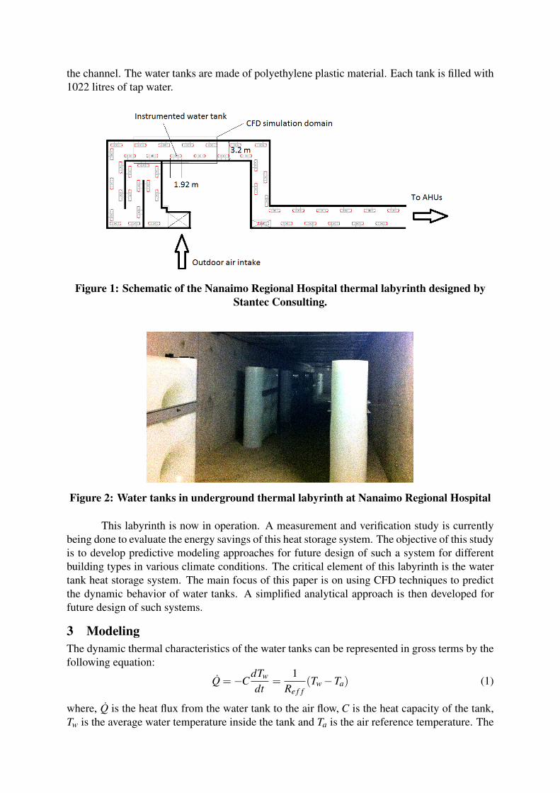
the channel. The water tanks are made of polyethylene plastic material. Each tank is filled with1022 litres of tap water.

Figure 1: Schematic of the Nanaimo Regional Hospital thermal labyrinth designed byStantec Consulting.

Figure 2: Water tanks in underground thermal labyrinth at Nanaimo Regional Hospital

This labyrinth is now in operation. A measurement and verification study is currentlybeing done to evaluate the energy savings of this heat storage system. The objective of this studyis to develop predictive modeling approaches for future design of such a system for differentbuilding types in various climate conditions. The critical element of this labyrinth is the watertank heat storage system. The main focus of this paper is on using CFD techniques to predictthe dynamic behavior of water tanks. A simplified analytical approach is then developed forfuture design of such systems.

3 ModelingThe dynamic thermal characteristics of the water tanks can be represented in gross terms by thefollowing equation:

Q̇ =−CdTw

dt=

1Re f f

(Tw−Ta) (1)

where, Q̇ is the heat flux from the water tank to the air flow, C is the heat capacity of the tank,Tw is the average water temperature inside the tank and Ta is the air reference temperature. The

effective R-value of the tank, Re f f , depends on three different physical phenomena: turbulentforced convection heat transfer between the tank surface and the air stream, solid conductionheat transfer in the polyethylene tank wall and natural convection of the water flow inside thetank. CFD can be used to calculate both forced and natural convection heat transfer phenom-ena. These two phenomena are effectively decoupled due to having substantially different timescales. Thus, the air flow simulations are first performed to calculate the air film R-value. Then,this R-value is used to calculate the natural convection heat transfer inside the water tank withan approximation for conduction heat transfer through the polyethylene walls. The OpenFOAM(2013) software package is used for these CFD modelings. OpenFOAM is an open-source toolfor solving partial differential equations with many different physical sub-models.

Air Flow ModelingThe rhoSimpleFoam solver of OpenFOAM is used for simulation of turbulent convection heattransfer. This is a compressible solver that solves continuity, Navier-Stokes and conservationof energy equations. The standard k-ε turbulence model is used (Launder & Spalding 1974).The kqRWallFunction turbulence wall function available in OpenFOAM is used for k,epsilonWallFunction is used for ε and mutkWallFunction is used for turbulentviscosity. This combination of wall functions result in imposing the zero gradient conditionfor turbulent kinetic energy on the wall and setting the ε and turbulent viscosity based on thelogarithmic law of the wall. Also, the production term for turbulent kinetic energy transportequation is modified near the wall (Versteeg & Malalasekera 2007). The problem is solvedwith a steady-state assumption and the SIMPLE algorithm for pressure corrections (Patankar &Spalding 1972). The total mass flow rate is set at the inlet boundary condition.

Validation Case

In order to validate the turbulent heat transfer modeling approach, a turbulent air boundarylayer over a heated flat plate is simulated. Seban & Doughty (1956) proposed the followingcorrelation for the non-dimensional heat transfer coefficient (Nusselt number):

Nux =hxxka

= 0.0236 Rex4/5 (2)

where hx is the local convection heat transfer coefficient hx = Q̇/A(Tw(x)−Ta), x is the spa-tial dimension starting from the flat plate leading edge, ka is the air conduction heat transfercoefficient and Rex = ρux/µ is the local Reynolds number. The CFD code described above isused to calculate the local heat flux. The simulation results are shown in Figure 3. Accordingto this figure, the CFD approach slightly under-predicts the heat transfer rate. The local heatflux is integrated over x to obtain the overall heat transfer rate over the flat plate. There is 15%discrepancy between the experimental and the CFD results in overall heat transfer rate in thisvalidation case.

Labyrinth Section Case

Only a section of the labyrinth is simulate to calculate the tank air film R-value. This sectionis shown in Figure 1. The tanks have a 1.92 m length and 1.92 m height. The geometry of thissection of the labyrinth is modeled in NX Unigraphics. This geometry is then exported to beused by the SnappyHexMesh grid generation utility of OpenFOAM. This utility generates anunstructured mesh (hexahedra, prisms, wedges, pyramids, tetrahedra and polyhedra) from an

0 5 10 15

x 105

0

500

1000

1500

2000

2500

Rex

Nu x

ExperimentCFD

Figure 3: Heat transfer coefficient as a function Reynolds number for turbulentconvection heat transfer over a heated flat plat.

arbitrary three-dimensional CAD surface. Figure 4 shows the details of the surface mesh in asection of the labyrinth.

Figure 4: Mesh details of the tank and channel wall surfaces.

The flow rate of each AHU is measured and logged in the building monitoring system.Simulations are performed with two flow rates: 10,000 CFM and 20,000 CFM. A constantvelocity inlet boundary condition is used to impose these flow rates.

In order to calculate the air film R-value, the temperature of one of the tanks (the controltank) is changed relative to the air flow temperature from 0◦C to 20◦C. The heat transfer betweenthe tank and the concrete slab is ignored. It is assumed that the concrete slab has the samesurface temperature as the surrounding air temperature. The simulations are performed withdifferent grids to ensure that the results are independent of the grid. The results of the finestgrid are shown here.

Figure 5 shows the contour plot of the heat flux on the control tank. According to thisfigure, the heat flux is higher on the leading face of the tank where the flow is impinging on thesurface. The total heat flux is plotted vs. the temperature gradient in Figure 6. The inverse of

the slope is the air film R-value: Rair f ilm = ∆T/Q̇.

Figure 5: The heat flux on the tank with different surface temperature.

0 5 10 15 200

200

400

600

800

1000

1200

∆T

Q̇

20,000 CFMy = 53x + 310,000 CFMy = 33x + 3

Figure 6: The total wall heat flux vs. temperature difference between the tank surfacetemperature and the air temperature.

Water Flow ModelingIn order to simulate the buoyant flow in the tank, the inside volume of the tank is meshed.The buoyantBoussinesqPimpleFoam solver of OpenFOAM is used for this simulation. This isan unsteady solver with a Boussinesq approximation for modeling the buoyancy effect. Thisapproximation is valid for low Mach number flows. This is a pressure-based solver that usesPIMPLE algorithm for pressure corrections(OpenFOAM 2013). PIMPLE algorithm is a com-bination of SIMPLE and PISO (Ferziger & Peri 2002) algorithm for unsteady flows. Since thetemperature gradients are not high enough, the flow velocity scale due to the buoyancy effectis low. Therefore, the flow field is laminar. This simulation only has no-slip wall boundarytype. In order to model the convection and conduction heat transfer into the tanks, a Robin-typeboundary condition is imposed on the walls for temperature:

k∂T∂n

= h(T −Ta) (3)

where T is wall temperature, ∂T∂n is the temperature gradient normal to the wall, k is the con-

duction heat transfer coefficient of the polyethylene, h is the convection heat transfer coefficientof the air film (1/Rair f ilm) and Ta is the air temperature. Using this boundary condition, thetemperature distribution inside the tank can be simulated by changing the surrounding air tem-perature.

The water flow field is initialized with T = 300 K. The air temperature is set to Ta =310 K at t = 0. The unsteady motion of the water flow inside the tank is simulated for 24 hours.Figure 7 shows the contour plot of the surface temperature after 5 hours. This figure showsthe temperature stratification throughout the tank due to the non-linear hydrodynamic buoyantflow. Using the above initial and boundary conditions, the simplified model of equation 1 has

XY

Z

T304303.5303302.5302301.5301300.5

Figure 7: Surface mesh and temperature contour plot of water at t=5h

the following analytical solution:

Ta−Tw(t)Ta−Tw(0)

= e−t/τ (4)

where τ = Re f fC is the characteristic time constant. The averaged water temperature of theCFD calculations can be used in the above equation to calculate the overall time constant forthermal charging and discharging of the tanks. Figure 8 shows the temporal variation of theaverage water tank temperature. Error bars represent twice the volume-averaged variance of thetemperature: T ′′2 =

∫(T 2

w −T 2w)dV/

∫dV . An exponential curve of the form of equation 4 is

fitted to the average temperature results as shown in Figure 8. This curve fit gives a value ofτ = 22.7 h for the time constant.

4 Experimental ResultsThis labyrinth is instrumented for dynamic control and long-term performance assessment.There are two temperature sensors inside the labyrinth for air temperature measurement andone temperature sensor inside one of the tanks. The location of the temperature sensors areshown in Figure 9. One of the air temperature sensors is upstream of the instrumented tank.

0 5 10 15 20 250

2

4

6

8

10

Time (h)

Ta−

Tw

Numerical ResultsExponential fit

y = 10e−0.044t

Figure 8: Temporal response of the average water tank temperature to the step change ofthe surrounding air temperature. Error bars represent twice of the temperature

variance.

Figure 9: Locations of the temperature sensors.This air temperature sensor is attached to the wall and does not provide the average air temper-ature upstream of the tank. Nevertheless, the output of this sensor and the water temperaturesensor are used to approximate the time constant of the water tanks. Figure 10 shows the diurnalvariation of the air and water temperature sensors for the date of 29/10/2013 – selected due tothe relatively high diurnal temperature variation that day. The instrumented water tank is lo-cated far downstream of the labyrinth outdoor air intake. Temperature variation in the labyrinthdecreases as the distance from the intake increase due to the thermal mass buffering effect.

The temperature data are used in equation 1 to find the time constant. The water tem-perature temporal derivative can be calculated numerically using a simple 2nd-order centralscheme. However, such a numerical integration can amplify the measurement error. In orderto alleviate this, a 6th-order polynomial is fitted to the water temperature data as shown in Fig-ure 10. The goodness of fit is R2 = 0.99. This polynomial is used to analytically calculatethe derivative. The difference between the water temperature and the air temperature is plottedagainst this derivative in Figure 11. These two parameters are linearly correlated; the slope ofthe fitted line is the time constant: τ ≈ 11.2 h.

The experimental result for the time constant is significantly different from the model

Figure 10: Storage tank water temperature and air flow temperature.prediction in the previous section. This is likely in part due to the inconsistencies in the refer-ence air temperature between the two calculations. As mentioned above, the air temperature isonly measured at one point close to the labyrinth concrete wall. Ideally, the average air tem-perature needs to be measured as well. Also, the flow rate sensors are based on the pressuredifference across the AHU supply fans. Further measurement is required to ensure the accuracyof these sensors.

At the same time, there are some important simplifications in the simulations. The heattransfer between the concrete wall and the water tank is ignored. As shown in Figure 2, the tanksare located on the concrete slabs without any insulation. Therefore, there exists a conductionheat transfer that depends on the contact resistance and the slab temperature. This informationis not currently available and will be addressed in future work. Another source of modelingerror is the underlying turbulence model in the air flow simulation. The tanks are inducing largescale turbulent structures in the flow field; Large-Eddy Simulation (LES) of the air flow is likelyto improve the results.

−0.2 −0.15 −0.1 −0.05 0 0.05−1.5

−1

−0.5

0

0.5

1

1.5

dTw

dt

Ta−

Tw

y = 11.23x + 0.7716

Figure 11: The correlation between the air-water temperature difference and the rate ofwater temperature change

5 Future DesignsIn this section a simplified mathematical approach is used to find the optimum time constantand operating condition for future design of a thermal labyrinth. Equation 1 has an analyticalclosed form solution for average water temperature as a function of the air temperature:

Tw(t) =1τ

e−t/τ

∫et/τTa(t)dt (5)

where τ = Re f fC. For simplicity, a cosine harmonic functional form is assumed for the airtemperature diurnal variation:

Ta = T0−δ cos(ωt) (6)

where T0 is the average daily temperature, ω = π/12 and t is the time in hours; δ is the fluc-tuation amplitude which is half of the difference between the maximum and minimum dailytemperature. Substituting equation 6 into equation 5, after integration and some simplifications,the following equation is obtained for the water tank temperature:

Tw = T0−δ∗ cos(ωt−θ)− δτ2ω2

1+ τ2ω2 e−t/τ (7)

The last term is the result of initial conditions and damps out quickly. The water temperaturefluctuation amplitude δ ∗ and the phase delay θ are as follows:

δ∗ =

δ√1+ τ2ω2

θ = sin−1(

τω√1+ τ2ω2

)(8)

These equations show that increasing τ results in decreasing the water tank temperature fluctu-ation amplitude. This is the case when either the capacity or R-value is large. The phase delayrepresents the buffering effect of the thermal mass. This number starts from θ = 0 for τ = 0and increases with increasing τ . It asymptotically approaches θ = π/2 as τ → ∞.

Substituting equation 7 into 1, the heat transfer rate from the water tank to labyrinth airflow can be calculated:

Q̇ =1

Re f f[δ ∗ cos(ωt−θ)−δ cos(ωt)] . (9)

According to this equation the heat transfer rate is inversely proportional to Re f f . However,for a constant capacity, increasing Re f f results in increasing τ which enhances the bufferingeffect of the thermal mass. In other words, the heat release happens when the air temperature isdecreasing and the thermal mass absorbs air flow heat when the temperature is increasing. Thiseffect is shown in Figure 12 for a daily averaged air temperature of T0 = 10◦C and fluctuationamplitude of δ = 5◦C. This figure suggests that there is an optimum value for the time constantτ that gives the best performance for the water tanks in the labyrinth.

The optimum performance of the water tanks also depends on the AHU set point tem-perature – relative to the mean outside air temperature – and the additional fan power due tothe presence of the tanks inside the channel. This extra fan power is related to the aerodynamicdrag force of the tank:

P = ηV̇FD

A(10)

0 5 10 15 20 25−2

0

2

Q̇(kW

)

Time (h)0 5 10 15 20 25

5

10

15

Ta

◦C

Increasing R

eff

Figure 12: Effect of changing the tank R-value on the diurnal heat flux from the tank.where η is the fan efficiency, V̇ is the volumetric flow rate through the labyrinth, A is the crosssection area of the labyrinth and FD is the drag force. This force can be easily obtained usingthe CFD model described in section 3. Knowing this parameter and the heat transfer rate, onecan define a daily cooling and heating performance factor for the water tanks in the labyrinth:

PF =

t2∫t1

Q̇dt

/ 24∫0

Pdt (11)

where [t1, t2] is the time frame when the air temperature is higher than the set-point temperature(Ta > Tset) for cooling performance factor. For the water tanks simulated in section 3, the dragforce is FD = 0.8 N. Assuming a fan efficiency of η = 0.7, the daily cooling performance factoris calculated. Figure 13 shows the contour plot of this parameter for δ = 5◦C as a function ofthe time constant and the AHU set-point temperature.

Figure 13 shows that the optimum value for the time constant is around 4 hours in-dependent of the operating conditions. Also, this figure shows that the optimum performancehappens when the average daily temperature is equal to the set-point temperature (T0 = Tset);in such a case, there is a balance between cooling and heating capacity that can be bufferedby the thermal mass effect of the labyrinth. On the other hand, as the difference between themean daily temperature and the AHU set-point temperature increases, the performance of thelabyrinth decreases. The above figure is for high outside air temperature fluctuations (δ = 5◦C)which is not always the case. Also as mentioned above, the water tanks that are further down-stream in the labyrinth are experiencing much smaller air temperature fluctuations. Therefore,under certain operating conditions the additional fan electricity consumption is higher than thethermal energy savings.

6 Conclusion and Future WorkIn this work, the dynamic performance of a water tank heat storage system in a building ther-mal labyrinth was investigated. The critical parameter in the dynamic behavior of a thermallabyrinth is the time constant which is a characteristic time scale for the charging and discharg-ing of thermal energy. This parameter was numerically and experimentally investigated. The

T0 − T

set

τ (h

)

−4 −2 0 2 4

2

4

6

8

10

12

14

16

18

20

40

60

80

100

120

Figure 13: The daily cooling performance factor of the water tank for δ = 5◦C

numerical approach comprises of two different CFD models: for the air flow and the buoyantwater flow. In the experimental approach, the water and air temperature are measured for aperiod of one day and used to approximate the time constant. There is a significant differencebetween the results of these two approaches and, in future work, we hope to address this dis-crepancy. More instrumentation such as averaging sensors for the air temperature and moreaccurate flow rate sensors will be installed in the labyrinth. Also, another water tank closer tothe labyrinth intake will be equipped with temperature sensors to enhance the temperature vari-ation resolution. The simulations will also be further developed with a better turbulence modeland considering the conduction heat transfer between the tanks and the concrete slabs.

7 AcknowledgmentThe financial support of NSERC and Sustainable Building Science Program is greatly appre-ciated. Also, the authors wish to thank Stantec Consulting and the Vancouver Island HealthAuthority for making design and operational data available.

8 ReferencesAllegrini, J., Dorer, V., Defraeye, T. & Carmeliet, J. (2012), ‘An adaptive temperature wall

function for mixed convective flows at exterior surfaces of buildings in street canyons’,Building and Environment 49(0), 55 – 66.

Braun, J. E. (2003), ‘Load control using building thermal mass’, Journal of Solar EnergyEngineering 125(3), 292–301.

Corgnati, S. P. & Kindinis, A. (2007), ‘Thermal mass activation by hollow core slab coupledwith night ventilation to reduce summer cooling loads’, Building and Environment42(9), 3285 – 3297.

Defraeye, T., Blocken, B. & Carmeliet, J. (2010), ‘CFD analysis of convective heat transfer atthe surfaces of a cube immersed in a turbulent boundary layer’, International Journal ofHeat and Mass Transfer 53(1-3), 297–308.

Defraeye, T., Blocken, B. & Carmeliet, J. (2011), ‘Convective heat transfer coefficients forexterior building surfaces: Existing correlations and CFD modelling’, Energy Conversionand Management 52(1), 512–522.

Dodoo, A., Gustavsson, L. & Sathre, R. (2012), ‘Effect of thermal mass on life cycle primaryenergy balances of a concrete- and a wood-frame building’, Applied Energy 92(0), 462 –472.

Ferziger, J. H. & Peri, M. (2002), Computational Methods for Fluid Dynamics, SpringerLondon, Limited.

Ghosal, M., Tiwari, G., Das, D. & Pandey, K. (2005), ‘Modeling and comparative thermalperformance of ground air collector and earth air heat exchanger for heating ofgreenhouse’, Energy and Buildings 37(6), 613 – 621.

Hardenberg, J. G. V. (1982), ‘Considerations of houses adapted to local climate a case studyof iranian houses in yazd and esfahan’, Energy and Buildings 4(2), 155 – 160.

IES - Virtural Environment (n.d.), http://www.iesve.com.

Kalogirou, S. A., Florides, G. & Tassou, S. (2002), ‘Energy analysis of buildings employingthermal mass in cyprus’, Renewable Energy 27(3), 353 – 368.

Kolokotroni, M., Webb, B. & Hayes, S. (1998), ‘Summer cooling with night ventilation foroffice buildings in moderate climates’, Energy and Buildings 27(3), 231 – 237.

Launder, B. E. & Spalding, D. B. (1974), ‘The numerical computation of turbulent flows’,Computer Methods for Applied Mechanics and Engineering 3(2), 268 – 289.

Meinders, E., Hanjalic, K. & Martinuzzi, R. (1999), ‘Experimental study of the localconvection heat transfer from a wall-mounted cube in turbulent channel flow’, Journal ofHeat Transfer-Transactions of the ASME 121(3), 564–573.

Newell, T. & Newell, B. (2011), ‘Thermal Mass Design’, ASHRAE Journal 53(3), 70+.

OpenFOAM (2013), The open source CFD Toolbox, OpenFOAM Foundations,http://www.openfoam.org/.

Patankar, S. V. & Spalding, D. B. (1972), ‘A calculation procedure for heat, mass andmomentum transfer in three-dimensional parabolic flows’, International Journal of Heatand Mass Transfer 15(10), 1787–1806.

Seban, R. A. & Doughty, D. L. (1956), ‘Heat transfer to turbulent boundary layers withvariable free-stream velocity’, Journal of Heat Transfer 78, 217223.

Spalart, P. (2000), ‘Strategies for turbulence modelling and simulations’, International Journalof Heat and Fluid Flow 21(3), 252 – 263.

Transient System Simulation Tool (n.d.), http://www.trnsys.com.

Tyacke, J. & Tucker, P. (2012), ‘LES of heat transfer in electronics’, Applied MathematicalModelling 36(7), 3112 – 3133.

Versteeg, H. K. & Malalasekera, W. (2007), An introduction to computational fluid dynamics:the finite volume method, Pearson Education Ltd., Harlow, England; New York.

Warwick, D. J., Cripps, A. J. & Kolokotroni, M. (2009), ‘Integrating active thermal massstrategies with HVAC systems: Dynamic thermal modelling’, International Journal ofVentilation 7(4), 345–367.

Yakhot, A., Anor, T., Liu, H. & Nikitin, N. (2006), ‘Direct numerical simulation of turbulentflow around a wall-mounted cube: spatio-temporal evolution of large-scale vortices’,Journal of Fluid Mechanics 566, 1–9.

Yang, L. & Li, Y. (2008), ‘Cooling load reduction by using thermal mass and nightventilation’, Energy and Buildings 40(11), 2052 – 2058.

Zhu, L., Hurt, R., Correia, D. & Boehm, R. (2009), ‘Detailed energy saving performanceanalyses on thermal mass walls demonstrated in a zero energy house’, Energy andBuildings 41(3), 303 – 310.