CFD Analysis of Sag Line Formation on the Zinc-coated ...
9
ISIJ International, Vol. 51 (2011), No. 1, pp. 115–123 1. Introduction A number of surface coating techniques are used in a va- riety of industrial fields such as paper, photographic film manufacturing, automobile, shipbuilding and home appli- ance industries. Among them, the galvanized steel surface has good corrosion resistance and it is produced by a con- tinuous hot-dip galvanizing process in which the fluid is molten zinc. In that process, a metallurgically clean and heat-treated steel strip is continuously passed through a molten zinc bath and is drawn up with the molten zinc ad- hered on both sides of the strip as schematically depicted in Fig. 1. In this case the thickness of the adhered zinc film is usually about 10 times thicker than desired thickness of around 20 m m. Such excessive zinc mass must be removed by mechanical, electromagnetic, or hydrodynamic opera- tions. Gas-jet wiping process is a hydrodynamic method to remove the excessive molten zinc adhered on the strip. In this process, a pair of opposing horizontal plane gas jets is located just above the bath, and the strip is vertically drawn up between the pair of opposing jets as shown in Fig. 1. The working gas is either air or nitrogen gas. This system is often referred to as “air-knife system” in the continuous hot-dip galvanizing industry. The gas wiping mechanism in the air-knife system has been well investigated theoretically and experimentally. Thornton and Graff 1) assumed that the final coating thickness is affected only by the longitudinal pressure gra- dient induced by the impinging jet on the strip. Tuck 2) have proposed a similar approach and investigated the stability CFD Analysis of Sag Line Formation on the Zinc-coated Steel Strip after the Gas-jet Wiping in the Continuous Hot-dip Galvanizing Process Hongyun SO, 1) Hyun Gi YOON 2) and Myung Kyoon CHUNG 1) 1) Department of Mechanical Engineering, KAIST, 373-1 Guseong-dong, Yuseong-gu, Deajeon 305-701 Republic of Korea. E- mail: [email protected] 2) Korea Atomic Energy Research Institute (KAERI), Daejeon, Republic of Korea. (Received on July 23, 2010; accepted on September 2, 2010 ) One of the surface defects on the steel strip surface after the gas-jet wiping employing an air-knife sys- tem in the continuous hot-dip galvanizing process is called sag lines or snaky coating. The sag line defect is the oblique patterns such as “W”, “V” or “X” on the coated surface. The present paper presents an analy- sis of the sag line formation and a numerical simulation of sag lines by using the numerical data produced by Large Eddy Simulation (LES) of the three-dimensional compressible turbulent flow field around the air- knife system. In order to simulate the sag line formation, a novel perturbation model has been developed to predict the variation of coating thickness along the transverse direction. The thickness obtained by the proposed model yields very similar results with those obtained by the conventional equation. It is observed that the coating thickness along the transverse direction is affected more by the pressure gradient than the surface shear stress in the stagnation region, while in the far field the shear stress becomes the major factor to determine the thickness. Finally, the three-dimensional coating surface was obtained by the present perturbation model. It was found that the sag line formation is determined by the combination of the instantaneous coating thickness distribution along the transverse direction near the stagnation line and the feed speed of the steel strip. The computed mean distance between the crests and the shape of the simulated sag show relatively good re- semblance with the real sag lines on the strip surface. KEY WORDS: air-knife; coating thickness; jet wiping; LES (large eddy simulation); perturbation method; sag line. 115 © 2011 ISIJ Fig. 1. Schematic diagram of a hot-dip galvanizing process with air knife.
Transcript of CFD Analysis of Sag Line Formation on the Zinc-coated ...
ISIJ International, Vol. 51 (2011), No. 1, pp. 115–123
1. Introduction
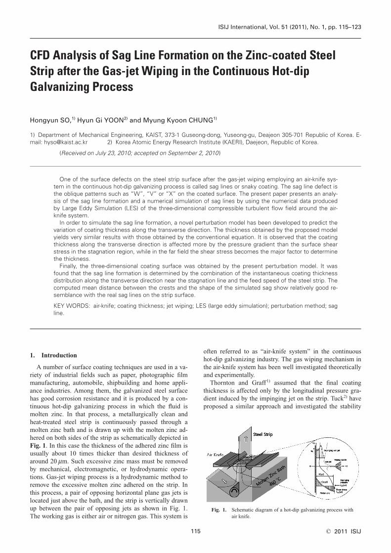
A number of surface coating techniques are used in a va-riety of industrial fields such as paper, photographic filmmanufacturing, automobile, shipbuilding and home appli-ance industries. Among them, the galvanized steel surfacehas good corrosion resistance and it is produced by a con-tinuous hot-dip galvanizing process in which the fluid ismolten zinc. In that process, a metallurgically clean andheat-treated steel strip is continuously passed through amolten zinc bath and is drawn up with the molten zinc ad-hered on both sides of the strip as schematically depicted inFig. 1. In this case the thickness of the adhered zinc film isusually about 10 times thicker than desired thickness ofaround 20 mm. Such excessive zinc mass must be removedby mechanical, electromagnetic, or hydrodynamic opera-tions. Gas-jet wiping process is a hydrodynamic method toremove the excessive molten zinc adhered on the strip. Inthis process, a pair of opposing horizontal plane gas jets islocated just above the bath, and the strip is vertically drawnup between the pair of opposing jets as shown in Fig. 1.The working gas is either air or nitrogen gas. This system is
often referred to as “air-knife system” in the continuoushot-dip galvanizing industry. The gas wiping mechanism inthe air-knife system has been well investigated theoreticallyand experimentally.
Thornton and Graff1) assumed that the final coatingthickness is affected only by the longitudinal pressure gra-dient induced by the impinging jet on the strip. Tuck2) haveproposed a similar approach and investigated the stability
CFD Analysis of Sag Line Formation on the Zinc-coated SteelStrip after the Gas-jet Wiping in the Continuous Hot-dipGalvanizing Process
Hongyun SO,1) Hyun Gi YOON2) and Myung Kyoon CHUNG1)
1) Department of Mechanical Engineering, KAIST, 373-1 Guseong-dong, Yuseong-gu, Deajeon 305-701 Republic of Korea. E-mail: [email protected] 2) Korea Atomic Energy Research Institute (KAERI), Daejeon, Republic of Korea.
(Received on July 23, 2010; accepted on September 2, 2010)
One of the surface defects on the steel strip surface after the gas-jet wiping employing an air-knife sys-tem in the continuous hot-dip galvanizing process is called sag lines or snaky coating. The sag line defect isthe oblique patterns such as “W”, “V” or “X” on the coated surface. The present paper presents an analy-sis of the sag line formation and a numerical simulation of sag lines by using the numerical data producedby Large Eddy Simulation (LES) of the three-dimensional compressible turbulent flow field around the air-knife system.
In order to simulate the sag line formation, a novel perturbation model has been developed to predict thevariation of coating thickness along the transverse direction. The thickness obtained by the proposed modelyields very similar results with those obtained by the conventional equation. It is observed that the coatingthickness along the transverse direction is affected more by the pressure gradient than the surface shearstress in the stagnation region, while in the far field the shear stress becomes the major factor to determinethe thickness.
Finally, the three-dimensional coating surface was obtained by the present perturbation model. It wasfound that the sag line formation is determined by the combination of the instantaneous coating thicknessdistribution along the transverse direction near the stagnation line and the feed speed of the steel strip. Thecomputed mean distance between the crests and the shape of the simulated sag show relatively good re-semblance with the real sag lines on the strip surface.
KEY WORDS: air-knife; coating thickness; jet wiping; LES (large eddy simulation); perturbation method; sagline.
115 © 2011 ISIJ
Fig. 1. Schematic diagram of a hot-dip galvanizing process withair knife.

of the coating thickness for long wavelength perturbations.Ellen and Tu3) have suggested a non-dimensional modelthat takes into account the surface shear stress and theirmodel gives significantly more accurate prediction of thefinal coating thickness. Also, Tu and Wood4) have experi-mentally demonstrated that the final coating thickness de-pends on both the pressure and shear stress distributions onthe strip surface. Although Tuck and Vanden-Broeck.5) andYoneda6) suggested that the final thickness depends on thesurface tension and the shear stress on the strip, recentlyGosset and Buchlin7) have shown that the surface tensiondoes not play any role in determining the final coatingthickness.
There have appeared several numerical simulations of thegas wiping process to predict the final coating thickness byusing CFD. One of the recent studies is that by Lacanette etal.8,9) who numerically simulated the final coating thicknessby using volume of fluid-large eddy simulation (VOF-LES)modeling. Their results were satisfactorily compared withtheir experimental data. They found that the coating thick-ness is independent of the nozzle-to-plate distance when itis smaller than 8 times of the nozzle slot width. Myrillas etal.10) tried to validate a model for the gas jet–liquid film in-teraction in the gas wiping process. In their study, theyfound that two-phase numerical simulations using LES ismore suited to model of the complex interaction than k–eturbulence model. Through these previous studies it can beconcluded that the dominant factors affecting the final coat-ing thickness are pressure gradient and shear stress on thestrip.
So far, most of the previous studies were focused on theaverage final coating thickness along longitudinal directionand their numerical and mathematical models are made intwo-dimensional domain. In spite of its good productivityand easy control of the zinc coating thickness, however, thecoated film surface after gas wiping has frequently three di-mensional surface defects such as dents, blow lines, pecu-liar features and sag-lines.11) Therefore, in order to obtain auniform coating on the strip, it is necessary to investigate indetails the three dimensional character of the coated surfaceafter the gas wiping process.
Among these surface defects, the sag lines (or snakycoating) cause many problems such as irregularity in theelectrical and thermal characteristics and the diffused re-flection on the coated surface. The snaky coating is thatwith an oblique patterns appearing on the coated film sur-face after the gas wiping process. Depending on its serious-ness, the snaky coating is usually classified into five gradesas shown in Fig. 2. The arrows in Fig. 2 indicate the mov-ing direction of steel strip. The first grade indicates that nosag line is observed on the surface. In the surface pattern ofthe 2nd grade, rather short sag lines appear irregularly, thusa pattern of sag lines is vaguely discernible. On the otherhand, the 3rd–5th grade snaky coatings reveal obliquecheckmark patterns such as “W”, “V” or “X” on the coatedsurface. Figure 3 demonstrates the micro-scale defects with3rd grade sag lines on the surface. The height from a valleyto the nearby crest is about 2–3 mm and the distance be-tween nearby crests is usually 3–4 mm. A principal cause ofsag line defect was firstly found by Yoon et al.12) They nu-merically simulated the turbulent flow field in the gas wip-
ing region using LES technique. And by scrutinizing theirsimulated flow field in details, they found that high and lowpressure points appear almost periodically along the im-pingement stagnation line across the strip surface. They re-vealed that such a pattern of periodical pressure distribu-tions moves alternatively sideways and together with thelongitudinal feed of the strip, it forms the sag lines ofcheckmark pattern on the surface. In a recent study,13) theyfurther showed that the snaky coating defect can be avoidedby suppressing the periodic variation of the surface pres-sure by utilizing a secondary parallel gas jet adjacent to themain jet. On the other hand, it was demonstrated that othersurface defects can be improved by controlling the alu-minum content and temperature of the bath14) or stirring themolten zinc in the bath.15)
The main objective of the present study is to predict thesag line formation along the transverse direction by analyz-ing numerical data obtained from Large Eddy Simulationfor the 3-D unsteady compressible flow filed around the air-knife system. Another objective is to suggest a new pertur-bation model to predict the variation of coating thicknessalong the transverse direction and to clarify the effects ofthe pressure gradient and surface shear stress for inducingthe sag line formation.
2. Numerical Analysis
In the present study, LES technique with the Smagorin-sky–Lilly sub-grid scale model is used to simulate the in-stantaneous flow field of the 3D unsteady compressible im-pinging jet.16) Boundary conditions and the computationaldomain are shown in Fig. 4. The transverse (i.e., horizontal)
ISIJ International, Vol. 51 (2011), No. 1
116© 2011 ISIJ
Fig. 2. Photograph of coated surface with different grade saglines. (a) 1st grade, (b) 2nd grade, (c) 3rd grade, (d) 4thgrade, (e) 5th grade.
Fig. 3. Micro-scale photograph of the coated surface with 3rdgrade sag lines.

width of the strip and the air-knife jet is 100 mm which istaken as the transverse length of the calculation domain.The opposing jet regions outside of the strip edge are notconsidered because the sag lines appear mostly in the inte-rior region. It is assumed that the mean flow field is homo-geneous in the transverse z-direction and Neumann condi-tion is given at both sides of the calculation domain. Thehomogeneity in the transverse direction has been testedwith a number of different transverse lengths, and it wasfound the 100 mm selected in the present study is wideenough to preserve the z-direction homogeneity of the flowfield.
In Fig. 4, the strip moves vertically upward in y-direc-tion, and the calculation domain in the vertical (i.e., longi-tudinal) direction is taken to be 60 mm. The atmosphericpressure condition is used at the top and bottom boundaries.The symbols d and L in Fig. 4 represent the jet slot widthand the distance from the nozzle exit to the moving plate,respectively. The origin of x-coordinate is located at thestrip surface, and that of y-coordinate is taken to be at thesame level of the lower lip of the jet slot (see Fig. 4). Andthe origin of z-coordinate is put at the right most end of thecomputational domain.
Working fluid is nitrogen gas used in the actual wipingprocess. In a previous experimental study, 3rd grade snakycoating was observed when an experimental air-knife sys-tem with d�1.5 mm and L�100 mm was operated at thestagnation pressure of 25 kPa and the stagnation tempera-ture of 340 K. These experimental conditions are used as abench-mark case to validate the present analysis model forpredictions of severe sag lines and the final coating thick-ness in the hot-dip galvanizing process. The surface of theplate is treated as a wall boundary moving at a speed of2.5 m/s in y-direction.
The smallest grid size is used near the nozzle exit and inthe jet-plate impinging region. It is determined to be aboutthe same size as the Taylor’s micro-length scale, l . In orderto estimate the Taylor’s micro-length scale, the energy dissi-pation rate is calculated by using the inviscid estimate ofKolmogorov given by e�u3/l, where u is the rms of thestream-wise velocity fluctuations and l is the integral lengthscale. Assuming that the turbulent velocity fluctuation isabout 10% of the jet exit velocity and that the integrallength scale is one half of the nozzle slot width, the Taylor’s
micro-length scale was estimated by e�15vu2/l2. In thisway, we obtained l�0.1 mm. Thus, the smallest grid spac-ing was taken to be 0.1 mm near the nozzle exit and in thejet-plate impinging region and the grid size was increasedat a successive rate in the �y-direction.
Time step of the unsteady solver was fixed to be D t�5.0�10�7 s which was determined from the smallest gridsize and the exit velocity of the plane jet. When the exit ve-locity is 230 m/s, the Courant number Ncourant�UD t/Dx is1.15 for the smallest grid size and it was found that theCourant number varies from about 0.5 to 1.5 in the wholecomputation domain in the present study. Considering thatthe appropriate range of the Courant number is generallyfrom 0.3 to 2 in LES simulation, the grid size and time stepused in the present study are suitable.16,17) Meanwhile,PISO algorism was used as the pressure–velocity couplingand bounded central differencing method was applied forthe discretization scheme.
3. Analytical Models for Predicting the Coating FilmThickness
3.1. Model to Calculate the Film Thickness Distribu-tion along the Longitudinal Direction
Several models have been suggested to predict the zincfilm thickness produced by the gas-jet wiping process. Oneof the first analytical models is the one proposed by Thorn-ton and Graff.1) They assumed that the final coating thick-ness is affected only by the pressure gradient induced bythe impinging jet on the strip. Tuck2) proposed a similar ap-proach and studied the stability of their solutions of thecoating thickness for long wavelength perturbations. Ellenand Tu3) suggested a non-dimensional model which for thefirst time takes into account the surface shear stress andtheir model significantly improved the prediction accuracyof the final coating thickness. Tu and Wood4) have experi-mentally demonstrated that the final coating thickness de-pends on both the pressure and shear stress distribution.
The principal step in predicting the coating thickness isthe calculation of the steady state flux of the molten zincadhered to the steel strip using a simplified form of theNavier–Stokes equation.3) The flow of molten zinc on thesurface is assumed to be steady, incompressible and creepflow. The fluid properties such as viscosity, density and
ISIJ International, Vol. 51 (2011), No. 1
117 © 2011 ISIJ
Fig. 4. Calculation domain and boundary conditions of the air knife system.

thermal conductivity are assumed constant. It is also as-sumed that surface tension and oxidation effects can beneglected. Using the coordinate system shown in Fig. 1, thegoverning equations and boundary conditions are summa-rized as follows.
Continuity and momentum equations:
...............................(1)
......(2)
Since the film thickness is very thin, it can be assumed thatthe pressure across the thin coating layer is constant and thevelocity component normal to the strip is zero. Then, Eqs.(1) and (2) can be simplified to the following Eqs. (3) and(4), respectively.
....................................(3)
.........................(4)
Now, Boundary conditions for these equations are
..............................(5)
..............................(6)
Integration of Eq. (4) with the boundary conditions Eqs. (5)and (6) leads to the velocity profile given by the followingEq. (7).
...(7)
Then, the volumetric liquid flow rate per unit width of thestrip becomes
.....(8)
Equation (8) is expressed with the normalized variables anddimensionless physical group as follows:
..............(9)
The normalized variables and dimensionless physical groupin Eq. (9) are defined as follows:
.......................(10)
Subscript 0 refers to the dragged film flow without wipingand 1 to the liquid phase. The solution of Eq. (9) for deter-
mining the film thickness along the longitudinal (vertical)direction d(y) is obtained by solving locally the cubic equa-tion and using the pressure gradient and shear stress distri-bution obtained by numerical simulation or measurement ofan impinging jet on the surface.
3.2. Model to Calculate the Film Thickness Distribu-tion along the Transverse Direction
Figure 5 demonstrates the distributions of the static wallpressure, its gradient and the wall shear stress along thelongitudinal direction computed by the present study.
At a certain transverse distance, it is convenient to repre-sent the local wall pressure gradient and local shear stressdenoted by ∇P̂ and T̂, respectively, as a sum of its meanover the transverse direction and the fluctuation values fromits mean. In this way, a perturbation model can be devel-oped as follows:
.................(11)
Here, – refers to the mean value over the transverse direc-tion and � to the fluctuation. Now, let’s consider the Eq. (9)in the following form.
...........(12)( ˆ )( ˆ ) . ( ˆ)( ˆ )1 1 5 2 003
0� � � �∇P T Qδ δ
∇ ∇ ∇ˆ ˆ ˆ ˆ ˆ ˆP P P T T T� � � � � �
∇∇ˆ ˆP
pT V� � �
ρττ
τ μ ρ1 0
0 1 1ggw
s
δμρ
δδδ
δ01
1 0 00 0
2
3� � � � �
VX
x
dQ
q
qq Vs
sgˆ
( ˆ ) ˆ . ˆ ˆ ˆ1 1 5 3 2 03 2� � � � �∇P T Qδ δ δ
q x y dx
V y yy
y
�
� � �
v( , )
( ) ( )( )
( )
0
231
2 3
δ
δτμ
δδ
μρ
∫s
w gg�dp
dy
⎛
⎝⎜⎞
⎠⎟
v( , ) ( )x y V xdp
dyx y x� � � � �s w
1 1
22
μτ ρ δg
⎛
⎝⎜⎞
⎠⎟⎛
⎝⎜⎞
⎠⎠⎟⎡
⎣⎢⎢
⎤
⎦⎥⎥
τ μw ( )yx
�∂∂v
v( , )x y Vx��0 s
1 2
2ρμρ
∂∂
∂∂
p
y x� �g
v
∂∂v
y�0
ux y
p
y x y
∂∂
∂∂
∂∂
∂∂
∂∂
⎛
⎝⎜
⎞
⎠⎟
vv
v v v� � � � �
1 2
2
2
2ρμρ
g
∂∂
∂∂
u
x y� �
v0
ISIJ International, Vol. 51 (2011), No. 1
118© 2011 ISIJ
Fig. 5. Wall static pressure, pressure gradient and shear stressalong the y-direction.

Here, it should be note that d̂0 is not the mean value of d̂over the transverse direction. Rather, it is thought of as anunperturbed value of the coating thickness corresponding tothe mean wall pressure gradient and the mean shear stress.In addition, local coating thickness (d̂ ) can be expressed asthe sum of the unperturbed state, d̂0 and the deviation part,d�.
...............................(13)
Then, the Eq. (9) is re-expressed by inserting the Eqs. (11)and (13) as follows:
.........................................(14)
Subtraction of Eq. (12) from Eq. (14) leads to the followingequation.
.........................................(15)
Here, if the perturbation magnitude is very small in com-parison with the mean value, one may assume that
.................(16)
Note that the fluctuation of pressure gradient is significantlylarger than the mean of static pressure gradient which valueis constant. Finally, the conditions in Eq. (16) simplify theEq. (15) to the following form:
............(17)
Therefore, the zinc coating thickness along the transversedirection is obtained by adding the average coating thick-ness to the fluctuation as
.............................(18)
This novel formula is very simple and compact to calculatethe film thickness in comparison with solving the thirdorder Eq. (9).
4. Computational Results and Discussions
Figure 5 represents the average static wall pressure, staticwall pressure gradient and wall shear stress distributionalong the longitudinal direction on the strip. The averagestatic pressure distribution on the strip is well described bya Gaussian law.4,18) The stagnation line corresponds to theplace where both the wall pressure gradient and the wallshear stress vanish. While the magnitude of the pressuregradient becomes negative above the stagnation line, thewall shear stress is positive, and vice versa under the stag-nation line. It may be interesting to note that the wall shearstress reaches its positive maximum significantly later thanthe negatively maximum value of the wall pressure gradi-ent. As will be seen later in Fig. 12, it is related to the for-
mation of the uneven coating surface.Figure 6 shows the average zinc coating thickness distri-
bution along the longitudinal direction. It was obtained bysolving Ep. (9) with the numerically computed average wallpressure gradient and surface shear stress. Here, it is worthnoting that the coating thickness is minimum where the av-erage wall pressure gradient has its maximum value. Inorder to compare the sensitivity of the coating thickness tothe pressure gradient and to the surface shear stress, thepressure gradient and the shear stress were arbitrarily in-creased by 50%, and the resulting coating thickness distri-butions are compared with those under the real pressuregradient and the shear stress in Fig. 7: The solid lines in thefigures indicate the results under the original pressure gra-dient and the shear stress, the dash-dotted lines show the re-sults with 50% increased pressure gradient, and the dottedlines demonstrates the results with 50% increased shearstress. As can be seen in Fig. 7(a), while a 50% increase inpressure gradient results in a reduction of 12% of the filmthickness, the same percentage increase in shear stress re-sults in a reduction of only 1% in the stagnation region.Therefore, it is apparent that the zinc coating thickness ismore affected by the pressure gradient than the surfaceshear stress in the stagnation region.1,9)
Figure 8 displays the instantaneous wall pressure con-tours on the xz-plane at y�1.4 mm. As can be seen in thefigure, the wall pressure varies almost periodically between5 kPa and 18 kPa along the impingement stagnation line onthe surface of the steel strip. It is also observed that thestatic pressure is distributed in a wavy form in the space be-tween the strip and the jet exit plane.
Figure 9 shows an instantaneous distribution of the wall
δ δ δ( ) ˆ ˆz � � �0
ˆ ( )ˆ ˆ . ˆ ˆ
{ ( ˆ ) ˆ ˆδ
δ δ
δ� �
� � �
� � � �z
P T
P
∇
∇03
02
02
1 5
3 1 TT ˆ }δ0 1�
ˆ ˆ ˆ ˆ ˆ ˆδ δ0 � � � � � �T T P P∇ ∇
( ˆ ˆ ){ ( ˆ ) ˆ ˆ ( ˆ ) ( ˆ ) }1 3 302
02 3� � � �� � � � �∇ ∇P P δ δ δ δ δ ∇∇ ˆ ( ˆ )
. ( ˆ ˆ ){ ˆ ˆ ( ˆ ) } .
P
T T
�
� � � �� � �
δ
δ δ δ0
3
021 5 2 1 5 ˆ̂ ( ˆ ) ˆT� � ��δ δ0
2 3 0
( ˆ )( ˆ ˆ )
. ( ˆ ˆ )( ˆ ˆ )
1
1 5
03
02
� � � � �
� � � � �
∇ ∇P P
T T
δ δ
δ δ �� � � � �3 2 00( ˆ ˆ )δ δ Q
ˆ ˆ ˆδ δ δ� � �0
ISIJ International, Vol. 51 (2011), No. 1
119 © 2011 ISIJ
Fig. 6. Averaged coating thickness along the y-direction afterwiping.
Fig. 7. Instantaneous coating thickness along z-direction at dif-ferent y-locations. (a) y�2.7 mm, (b) y�20 mm. —:thickness from Eq. (17) under original ∇P and T, – -:thickness with 50% increased ∇P, - -: thickness with50% increased T.
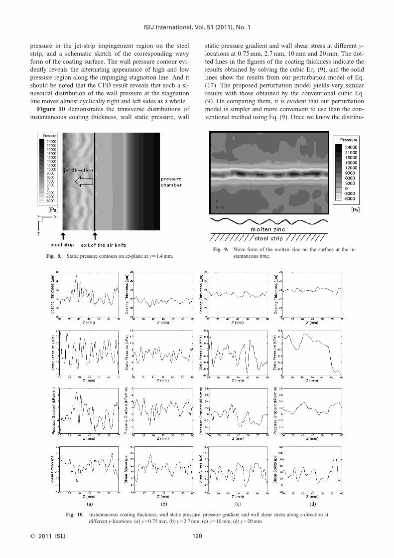
pressure in the jet-strip impingement region on the steelstrip, and a schematic sketch of the corresponding wavyform of the coating surface. The wall pressure contour evi-dently reveals the alternating appearance of high and lowpressure region along the impinging stagnation line. And itshould be noted that the CFD result reveals that such a si-nusoidal distribution of the wall pressure at the stagnationline moves almost cyclically right and left sides as a whole.
Figure 10 demonstrates the transverse distributions ofinstantaneous coating thickness, wall static pressure, wall
static pressure gradient and wall shear stress at different y-locations at 0.75 mm, 2.7 mm, 10 mm and 20 mm. The dot-ted lines in the figures of the coating thickness indicate theresults obtained by solving the cubic Eq. (9), and the solidlines show the results from our perturbation model of Eq.(17). The proposed perturbation model yields very similarresults with those obtained by the conventional cubic Eq.(9). On comparing them, it is evident that our perturbationmodel is simpler and more convenient to use than the con-ventional method using Eq. (9). Once we know the distribu-
ISIJ International, Vol. 51 (2011), No. 1
120© 2011 ISIJ
Fig. 8. Static pressure contours on xz-plane at y�1.4 mm.Fig. 9. Wave form of the molten zinc on the surface at the in-
stantaneous time.
Fig. 10. Instantaneous coating thickness, wall static pressure, pressure gradient and wall shear stress along z-direction atdifferent y-locations. (a) y�0.75 mm, (b) y�2.7 mm, (c) y�10 mm, (d) y�20 mm.

tions of the wall pressure gradient and shear stress on thestrip from experimental or numerical study, variations ofthe coating thickness along both the longitudinal and trans-verse directions are readily obtained by using Eqs. (12),(17) and (18).
Location at y�0.75 mm in Fig. 10(a) coincides with thecenter of the jet slot. The jet collides with the strip surfacein the closest distance. Here the wall pressure varies almostperiodically in the transverse direction. Comparing thetransverse variations of the wall pressure and the coatingthickness, one can conclude that the coating thickness is lo-cally thickest where the wall pressure reaches its local mini-mum: It is physically evident that the molten zinc is re-moved at a maximum rate where the wall pressure becomeslocally strongest. When one compares the magnitude of thewall shear stress at this location with those at other loca-tions of Figs. 10(b)–10(d), the wall shear stress is relativelyvery small. Therefore, along the impinging stagnation line,the wall shear stress does not have any effect on removingthe molten zinc, and the coating thickness is determinedmostly by the wall pressure. Here, a notable observation isthat the distributions of the coating thickness and the pres-sure gradient are nearly the same. This implies that thecoating thickness is more directly related to the pressuregradient rather than the wall pressure itself.
Now, consider the case of Fig. 10(b) at y�2.7 mm thatstill belongs to the impinging stagnation region. The wallshear stress has significantly large magnitude in comparisonthat at y�0.75 mm. Even with such large magnitude of thewall shear stress, the same relations as in case (a) can beobserved, although weakly related for this case, between thecoating thickness and the wall pressure, and between thecoating thickness and the wall pressure gradient. Therefore,in the jet impinging zone, the wall pressure and the pressuregradient are dominant variables for the zinc film thickness.This result is similar to the recent observation of Lacanetteet al.9) in which the sensitivity of their analytical model ofcoating thickness to pressure gradient and shear stress hasbeen investigated.
On the other hand, when the strip moves up farther than10 mm, say, the wall pressure becomes vanishingly small,while the magnitude of wall shear stress does not changemuch as can be seen in Figs. 10(c) and 10(d). Therefore,the flow field condition to determine the coating thicknessis obviously different from that in the impinging stagnationregion. In contrast to the impinging stagnation region, themain wiping factor in the far field is evidently the wallshear stress. Since, farther downstream from the impinge-ment region after colliding with the strip, the impinged gasmoves in the direction parallel to the strip in a manner ofwall jet and the wall static pressure asymptotes gradually tothe ambient pressure, the molten zinc is subjected to the ef-fect of the surface shear stress only. In fact, Figs. 10(c) and10(d) reveal that the coating thickness is nearly inverselyproportional to the wall shear stress. Figure 7(b) shows thequantitative comparison the contribution to the zinc coatingthickness from the pressure gradient and the shear stress inthe far field. While a 50% increase in wall shear stress re-sults in a reduction of 6% of the film thickness, the samepercentage increase in the pressure gradient does not affectat all the film thickness after wiping. This relation can also
be theoretically deduced from Eq. (17): When the pressuregradient is vanishingly small, the only variable to affect thefinal coating thickness is the wall shear stress.
Figure 11 shows the variation of the transverse distribu-tion of the instantaneous coating thickness along the longi-tudinal direction. Initially in the impinging stagnation re-gion, the coating thickness is notably very uneven, but asthe strip travels upward such unevenness gradually be-comes weak. Quantitatively, the rms variation of the coatingthickness at y�2.7 mm is 1.5 mm and gradually it decreasesto 0.8 mm at y�20 mm.
ISIJ International, Vol. 51 (2011), No. 1
121 © 2011 ISIJ
Fig. 11. Variation of the transverse coating thickness distributionalong y-direction.
Fig. 12. Three dimensional zinc coating thickness distributionon a strip surface. (a) 3-D oblique view, (b) 3-D sideview.
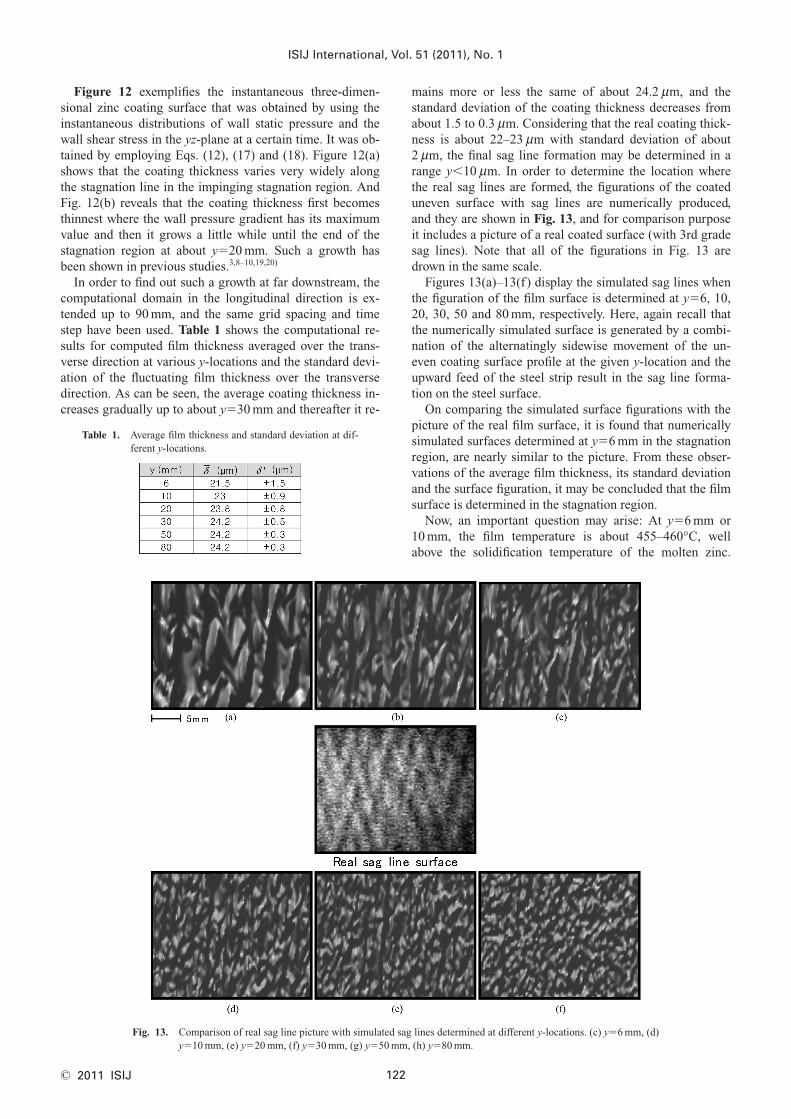
Figure 12 exemplifies the instantaneous three-dimen-sional zinc coating surface that was obtained by using theinstantaneous distributions of wall static pressure and thewall shear stress in the yz-plane at a certain time. It was ob-tained by employing Eqs. (12), (17) and (18). Figure 12(a)shows that the coating thickness varies very widely alongthe stagnation line in the impinging stagnation region. AndFig. 12(b) reveals that the coating thickness first becomesthinnest where the wall pressure gradient has its maximumvalue and then it grows a little while until the end of thestagnation region at about y�20 mm. Such a growth hasbeen shown in previous studies.3,8–10,19,20)
In order to find out such a growth at far downstream, thecomputational domain in the longitudinal direction is ex-tended up to 90 mm, and the same grid spacing and timestep have been used. Table 1 shows the computational re-sults for computed film thickness averaged over the trans-verse direction at various y-locations and the standard devi-ation of the fluctuating film thickness over the transversedirection. As can be seen, the average coating thickness in-creases gradually up to about y�30 mm and thereafter it re-
mains more or less the same of about 24.2 mm, and thestandard deviation of the coating thickness decreases fromabout 1.5 to 0.3 mm. Considering that the real coating thick-ness is about 22–23 mm with standard deviation of about2 mm, the final sag line formation may be determined in arange y�10 mm. In order to determine the location wherethe real sag lines are formed, the figurations of the coateduneven surface with sag lines are numerically produced,and they are shown in Fig. 13, and for comparison purposeit includes a picture of a real coated surface (with 3rd gradesag lines). Note that all of the figurations in Fig. 13 aredrown in the same scale.
Figures 13(a)–13(f) display the simulated sag lines whenthe figuration of the film surface is determined at y�6, 10,20, 30, 50 and 80 mm, respectively. Here, again recall thatthe numerically simulated surface is generated by a combi-nation of the alternatingly sidewise movement of the un-even coating surface profile at the given y-location and theupward feed of the steel strip result in the sag line forma-tion on the steel surface.
On comparing the simulated surface figurations with thepicture of the real film surface, it is found that numericallysimulated surfaces determined at y�6 mm in the stagnationregion, are nearly similar to the picture. From these obser-vations of the average film thickness, its standard deviationand the surface figuration, it may be concluded that the filmsurface is determined in the stagnation region.
Now, an important question may arise: At y�6 mm or10 mm, the film temperature is about 455–460°C, wellabove the solidification temperature of the molten zinc.
ISIJ International, Vol. 51 (2011), No. 1
122© 2011 ISIJ
Table 1. Average film thickness and standard deviation at dif-ferent y-locations.
Fig. 13. Comparison of real sag line picture with simulated sag lines determined at different y-locations. (c) y�6 mm, (d)y�10 mm, (e) y�20 mm, (f) y�30 mm, (g) y�50 mm, (h) y�80 mm.

Then why could the film surface determined at such hightemperature be unchanged downstream? In order to theo-rize the problem, let us consider a local time scale in themolten zinc film. In the stagnation region, major parametersfor the relaxation of the molten zinc film, highly strained bythe static pressure, are the local wall shear stress and theviscosity of the molten zinc. Therefore, the relaxation timescale is given by the following equation.21,22)
...............................(19)
Physically, the relaxation time indicates the time durationwithin which the very viscous molten zinc film completesto be deformed responding to the local external disturbancesuch as the static pressure and wall shear stress. As can beconfirmed in Fig. 5, since the wall shear stress is very closeto zero in the impingement region, the relaxation time is ina range trelax0.5 s. This means that the surface figurationof the zinc film formed in the impingement region main-tains its configuration for a while during its upward move-ment. And after the relaxation time of about 0.5 s, the steelstrip has moved upward by about 1.2 m where the film tem-perature dropped down below the solidification tempera-ture. Following this reason, we may conclude that the un-even film surface figuration is determined in the stagnationregion. In addition, the mean distance between the nearbycrests is 4 mm�10% which is nearly the same as the exper-imentally measured distance in Fig. 3.
5. Conclusion
The sag line formation on galvanized strip surfacecaused by the gas jet-wiping process has been studied bynumerical simulation and analytical modeling. In order tosimulate the sag line formation after gas wiping in a contin-uous hot-dip galvanizing process, CFD simulation for the3-D compressible turbulent flow field around the air knifehas been carried out by using the commercial code, FLU-ENT. LES technique was used to simulate the unstable andcomplex 3-D flow field. It was confirmed that the periodi-cally alternating sidewise movement of the peak pressurepoints along the transverse stagnation line with the upwardmoving steel strip at a constant speed results in the sag lineformation on the zinc coating strip surface.
A simple mathematical model has been suggested to pre-dict the coating thickness distribution along the transversedirection. The coating thickness calculated by our newmodel shows good agreement with that obtained by the ex-isting model. Our proposed model is an explicit formula topredict the film thickness, and it reveals better understand-ing about the relationship between the unevenness of thezinc film thickness and wiping parameters such as staticpressure gradient and wall shear stress.
Finally, the 3-D uneven surface figuration with the saglines on the zinc coated steel strip was successfully gener-ated by using the perturbation model and wiping factors ob-tained from our numerical simulation. Relaxation time isintroduced to interpret the position where the sag lines aredetermined.
Nomenclature
l : Taylor’s micro-length scale (m)e : Turbulent energy dissipation rate (m2/s2)u : Liquid velocity in x-direction (m/s)v : Liquid velocity in y-direction (m/s)x : Distance of horizontal direction (m)y : Distance of vertical direction (m)g : Acceleration of gravity (m/s2)r : Density of liquid zinc (kg/m3)m : Dynamic viscosity of liquid zinc (Pa · s)p : Impinging pressure (Pa)
Vs : Moving velocity of the steel strip (m/s)tw : Wall shear stress (Pa)d : Coating thickness (m)q : Volumetric liquid flow rate per unit width of strip
(m2/s)d : Nozzle slot height (m)
∇P̂ : Dimensionless pressure gradient in y-direction∇P̄̂ : Mean of dimensionless pressure gradient over the
z-direction∇P� : Fluctuation of dimensionless pressure gradient over
the z-directionT̂ : Dimensionless shear stressT̂̄ : Mean of dimensionless shear stress
T̂� : Fluctuation of dimensionless shear stress
d : Dimensionless coating thicknessd0 : Unperturbed dimensionless coating thicknessd� : Deviation value over the unperturbed dimensionless
coating thickness
REFERENCES
1) J. A. Thornton and H. F. Graff: Metall. Mater. Trans. B, 7B (1976),607.
2) E. O. Tuck: Phys. Fluids, 26 (1983), 2352.3) C. H. Ellen and C. V. Tu: J. Fluid. Eng., 106 (1984), 399.4) C. V. Tu and D. H. Wood: Exp. Therm. Fluid Sci., 13 (1996), 364.5) E. O. Tuck and J. M. Vanden-Broeck: AIChE. J., 30 (1984), 808.6) H. Yoneda: Master’s Thesis, University of Minnesota, (1993).7) A. Gosset and J. M. Buchlin: J. Fluid. Eng., 129 (2007), 466.8) D. Lacanette, S. Vincent, E. Arquis and P. Gardin: ISIJ Int., 45
(2005), No. 2, 214.9) D. Lacanette, A. Gosset, S. Vincent J. M. Buchlin and E. Arquis:
Phys. Fluids, 18 (2006), 042103.10) K. Myrillas, A. Gosset, P. Rambaud and J. M. Buchlin: Eur. Phys. J.
Special Topics, 166 (2009), 93.11) N. Y. Tang and F. N. Coady: Galvanizer’s Association Meeting, Port-
land, Oregon, (2001).12) H. G. Yoon, G. J. Ahn, S. J. Kim and M. K. Chung: ISIJ Int., 49
(2009), No. 11, 1755.13) H. G. Yoon and M. K. Chung: ISIJ Int., 50 (2010), No. 5, 752.14) N. Y. Tang: Metall. Mater. Trans. B, 30B (1999), 144.15) L. Bordignon: ISIJ Int., 41 (2001), No. 2, 168.16) H. K. Versteeg and W. Malalasekera: Computational Fluid Dynam-
ics, Pearson Prentice Hall, London, (2007), 98.17) J. H. Ferziger and M. Peric: Computational Methods for Fluid Dy-
namics, Springer, Berlin, (2002), 143.18) S. Beltaos and N. Rajaratnam: J. Hydraulic Res., 11 (1973), 29.19) S. B. Kwon, Y. D. Kwon, S. J. Lee S. Y. Shin and G. Y. Kim: J.
Mech. Sci. Technol., 23 (2009), 3471.20) H. Y. So, H. G. Yoon and M. K. Chung: Asia-Pacific Galvanizing
Conf. 2009, CSSK, Jeju, (2009), A-13.21) R. B. Bird, R. C. Armstrong and O. Hassager: Dynamics of Poly-
meric Liquids Volume 1 Fluid Mechanics, John Wiley & Sons, NewYork, (1987), 227.
22) J. P. Rothstein and G. H. McKinley: J. Non-Newtonian Fluid Mech.,86 (1999), 61.
trelaxw
�μ
τ
ISIJ International, Vol. 51 (2011), No. 1
123 © 2011 ISIJ