Centro de Estudos da União Europeia (CEUNEUROP) Faculdade ...

Centro de Estudos da União Europeia (CEUNEUROP) Faculdade de Economia da Universidade de Coimbra

Av. Dias da Silva, 165-3004-512 COIMBRA – PORTUGAL e-mail: [email protected] website: www4.fe.uc.pt/ceue

Túlio Cravo and Elias Soukiazis

Human capital as a conditioning factor to the convergence process among the Brazilian States

DOCUMENTO DE TRABALHO/DISCUSSION PAPER Nº 35

(FEBRUARY, 2006)

Nenhuma parte desta publicação poderá ser reproduzida ou transmitida por qualquer forma ou processo, electrónico, mecânico ou fotográfico, incluindo fotocópia, xerocópia ou gravação, sem autorização PRÉVIA.

COIMBRA — 2006

Impresso na Secção de Textos da FEUC

1

Human capital as a conditioning factor to the convergence process among the Brazilian States1. Túlio Cravo and Elias Soukiazis Abstract

This paper examines the convergence process among the Brazilian states using different concepts of convergence and giving special attention to the role of human capital as the conditioning factor to convergence. Different measures of human capital are used in the estimation of the convergence equations and the results show that they play a significant role in explaining the improvement of the standards of living of the Brazilian population. An interesting finding is that different levels of human capital have different impacts on the growth of per capita income depending on the level of development of the Brazilian states. Lower levels of human capital explain better the convergence process among the less developed states and higher levels of human capital are more adequate for controlling differences in the “steady-states” of the more developed Brazilian regions. The impact of the intermediate levels of human capital on growth is stronger in all samples. JEL classification: O, O1, O15 Keywords: absolute and conditional convergence, club-convergence, σ- convergence, human capital, panel data. Author for correspondence: Soukiazis Elias, Faculdade de Economia, Universidade de Coimbra, Av, Dias da Silva, 165, 3004-512 Coimbra, Portugal, Tel, + 351 239 790 534, Fax + 351 239 40 35 11, e-mail: elias@fe,uc,pt.

1 This study is a reformulated part of the MA dissertation elaborated by Túlio Cravo and supervised by Elias Soukiazis.

2

1. Introduction

Since the 1980s, the convergence phenomenon has been widely discussed in the

growth literature and many concepts related to convergence in per capita income or

productivity (output per worker) were developed to explain economic growth, especially

regional growth. Most empirical studies have shown that convergence is conditional

rather than absolute. The former is the argument of the endogenous growth theory with

increasing returns to scale properties (mostly in human capital and technology), the latter

is the argument of the neoclassical approach to growth with constant returns to scale

properties (or diminishing returns to capital) and exogenous technical progress.

Therefore, the fundamental problem in growth theory consists in finding the conditioning

factors that better explain the convergence process among different economies (states or

regions). Among a variety of studies, the endogenous growth approach advocates that

human capital is the engine of growth and that convergence is higher when this factor is

introduced into the convergence equation. Convergence has been found to run at 2%

annual rate, and this is a stylized fact either in samples with countries or in samples with

different regions.

The aim of this study is to test the importance of human capital in the

convergence process across the Brazilian states over the period 1980-2000, by using a

panel data approach. Different measures of human capital are used in the estimation

process, such as, basic schooling expressed by the illiteracy rate, secondary school

enrolment rate, and total years of school attainment, as well as, a variable which

measures the efficiency of scientific work, expressed by the publication rates of articles

in international journals. The purpose of the study is to measure the different impacts of

the different levels of human capital on the growth of per capita income among the

Brazilian states, how do they affect the convergence rate and if different education levels

affect differently the samples of regions with dissimilar levels of development. To our

knowledge this gradual testing of different levels of human capital on growth and

convergence has not been considered systematically, especially for the Brazilian

economy.

3

To study the convergence process across the Brazilian states giving special

attention to human capital, we structure the paper as follows: Section 2 explains the

various concepts of convergence that are normally used in the growth literature. Section 3

describes the convergence model derived from the Solow´s growth theory. Section 4

discusses the importance of human capital on economic growth. Section 5 explains the

data and the samples considered in the empirical analysis. Section 6 explains the

disparities among the Brazilian states in terms of wealth and education standards and

gives evidence on σ-convergence. Section 7 tests the hypothesis of absolute convergence.

Section 8 tests the hypothesis of conditional convergence assuming that growth is

conditioned to different levels of human capital. The final section concludes the main

findings,

2. Concepts of convergence

Many concepts of convergence have been used to explain whether different

economies tend to equalise their levels of economic development. Following Galor

(1996), the controversy across different concepts has been largely empirical, focusing on

the validity of the following hypotheses:

(i)The absolute convergence hypothesis: per capita income of countries converge to one

another in the long run independently of their initial conditions. In other words, all

economies converge to the same steady-state. This hypothesis is derived from the

Solow`s growth model and can be tested empirically by the following regression

TtititiTti yba

Tyy

++ ++=−

00

00,,

,, lnlnln

ε (1)

where y is per capita income, i the individual economy, b = (1-e-βT) the convergence

coefficient, β=-ln(1-b)/T the convergence rate, t0 the initial period and T the time length

that the per capita income growth rate is measured. If b occurs with a negative sign (b<0)

in the estimation process then it can be said that the data produces absolute convergence.

4

(ii) The conditional convergence hypothesis: per capita incomes of countries that are

identical in their structural characteristics (preferences, technologies, human capital,

government policies, etc) converge to one another in the long run independently of their

initial conditions. On the contrary to the absolute convergence, this hypothesis states that

economies have different structures and therefore they converge to different steady-

states. Or alternatively, economies will converge to the same steady-state only if they are

similar to their structural characteristics. As Barro (1991) and Sala-i-Martin (1996)

suggested, the hypothesis of conditional convergence can be tested by estimating the

following equation

TtitititiTti Xyba

Tyy

++ +++=−

000

00,,,

,, lnlnlnln

εψ (2)

where X is a vector of factors that allow to control differences across economies. If b<0

and ψ ≠ 0 we can say that the data exhibits conditional convergence. On the other hand,

b<0 and ψ = 0 imply that convergence is absolute.

(iii)The convergence- club hypothesis: per capita income of countries that are identical in

their structural characteristics converge to one another in the long-run provided that their

initial conditions (starting levels of per capita income) are similar as well. This

hypothesis is consistent with the phenomena of polarization, clustering or persistent

poverty situation.

(iv) Beyond all these hypotheses, listed by Galor, the σ-convergence concept is also used

to measure the dispersion of per capita income over time, among different economies. A

group of economies is converging in this sense if the dispersion of their per capita income

tends to decrease over time. The coefficient of variation is normally used to test the

hypothesis of σ-convergence, given by the ratio of the standard deviation to the sample

mean. This concept was first introduced by Barro (1991), to distinguish it from β-

convergence associated to conditional convergence. As Barro argues, σ-convergence is a

necessary but not a sufficient condition for β-convergence to occur. Both concepts are

useful, giving different information about the convergence phenomenon.

5

All these alternative concepts will be used to test the hypothesis of convergence

between the Brazilian states.

3. Description of the convergence model2

The concept of β convergence is derived from the Solow (1956) neoclassical

growth model based on the Cobb-Douglas production function with labour-augmenting

technical progress given by:

( ) ( ) ( ) ( )[ ] 10,1 <<= − ααα withtLtAtKtY (3)

where is output, Y K and L are the factor inputs, capital and labour, respectively, A

measures the cumulative effect of technical progress through time, α is the capital

elasticity with respect to output and t is time.

The model assumes that L and A grow exogenously at constant rates and ,

given by and

n g

( ) ( ) nteLtL 0= ( ) ( ) gteAtA 0= , respectively. On the other hand, saving is a

constant fraction of output , (s 10, <<= ssYS ) and K depreciates at a constant

exogenous rate δ , therefore, KIdtdKK δ−==& . Accordingly, a constant amount of

capital Kδ , in each period t , is not used.

Under the standard neoclassical assumption of constant returns to scale, the

production function, in terms of efficient units of labour, is given by

withky ,α=ALYy = and

ALKk = (4)

The dynamic specification of the model with technical progress takes the

following form:

( ) ( ) ( ) ( )tkgntkstk δα ++−=& (5)

Since in the steady-state the rate of growth of capital stock is zero ( 0=k& ), *k

satisfies the following condition:

2 The description of the convergence model follows closely Islam (1995).

6

( ) ( ) ( )⇔++= tkgntks ** δα α

δ

−

⎟⎟⎠

⎞⎜⎜⎝

⎛++

=1

1

*

gnsk (6)

Substituting the expression found for *k into the production function (4) we

derive, analogously, the steady-state value of output

αα

δ

−

⎟⎟⎠

⎞⎜⎜⎝

⎛++

=1

*

gnsy (7)

From the definition of output in terms of efficient units of labour, ALYy = , and the

expression found for the level of output in the steady-state, equation (7), it is possible to

derive an expression for the steady-state per capita income:

( )( ) ( ) ( ) ( δ

αα

αα

++⎟⎠⎞

⎜⎝⎛−

−⎟⎠⎞

⎜⎝⎛−

++=⎥⎦

⎤⎢⎣

⎡ gnsgtAtLtY ln

1ln

10lnln ) (8)

In this equation is a constant, since the exogenous rate of technical progress is

assumed to be equal in all economies and t is fixed in cross-section regressions. On the

other hand, may differ across economies, since it reflects not only the level of

technology but also resource endowments, institutions, economic conditions, among

others (Mankiw et al., 1992). Accordingly, the term

gt

( )0A

( )0ln A can be decomposed into two

parts: the first is a constant (γ ) and the other is stochastic (ε ), representing a country (or

region) specific shock:

( ) εγ +=0ln A (9)

Substituting into equation (8) and inserting into the constant term ( )0ln A gt γ ,

we obtain the following expression:

( )( ) ( ) ( ) εδ

αα

ααγ +++⎟

⎠⎞

⎜⎝⎛

−−⎟

⎠⎞

⎜⎝⎛

−+=⎥

⎦

⎤⎢⎣

⎡gns

tLtY ln

1ln

1ln (10)

A cross-section estimation of equation (10) is heavily dependent on the assumption that

and are not correlated with the error term (s n ε ). In general, this is not a convincing

argument that saving and population (labour) growth rates will not be influenced by the

factors included in . This problem is solved when panel regression (instead of cross-( )0A

7

section) is used, allowing for country (or region) specific effects (fixed or random)

providing, therefore, a better control for the technology shift term (ε ).

Having this in mind, we consider the equation describing the out of steady-state

behaviour of per capita income:

( ) ( ) ( )([ tyydt

tyd lnlnln * −= β )] (11)

where β = ( δ++ gn )( α−1 ) is the rate of convergence dependent on the rate of growth

of population, technology, capital depreciation and the output elasticity with respect to

capital. This equation implies that:

( ) ( ) ( )1*

2 lnln1ln tyeyety TT ββ −− +−= (12)

where ( )1ty is income per effective worker at some initial point of time and 12 ttT −=

the considered period.

Subtracting ( )1ln ty from both sides of equation (12) we obtain a specification that

represents a partial adjustment process:

( ) ( ) ( ) ( )[ ]1*

12 lnln1lnln tyyetyty T −−=− −β (13)

In this model the growth of income per effective worker between the period

and is determined by the distance of its initial level and the steady-state value.

2t

1t

Substituting for *y we obtain the following expression:

( ) ( ) ( ) ( ) ( ) ( )⎥⎦

⎤⎢⎣

⎡−++⎟

⎠⎞

⎜⎝⎛−

−⎟⎠⎞

⎜⎝⎛−

−=− −112 lnln

1ln

11lnln tygnsetyty T δ

αα

ααβ (14)

In this equation the growth of income per effective worker is explained solely by

its initial value (the unique factor of convergence), assuming ( δ+g ) to be the same for

all economies and saving and population growth rates are taken to be equal to the

respective averages over the considered period. This is known as the neoclassical

hypothesis of absolute or unconditional convergence.

The neoclassical convergence equation (14) defined in terms of income per

effective worker does not show the correlation between the unobservable and the ( )0A

8

observed included variables. This problem is more apparent when the equation is

expressed in terms of per capita income.

Starting from the definition of income per worker ( ) ( )( ) ( )

( )( ) ( ) tgeAtL

tYtLtA

tYty0

== ,

and getting logs we obtain:

( ) ( )( ) ( ) ( ) ( ) ( ) gtAtytytAtLtYty −−=⇔−⎥⎦

⎤⎢⎣

⎡= 0lnlnlnlnlnln (15)

where is per capita income. Substituting for ( )ty ( )ty into equation (15) we obtain the

usual convergence equation in per capita income terms:

( ) ( ) ( ) ( ) ( ) ( )

( ) ( ) ( ) ( ) ( ) tiTTT

TT

vtetgAetye

gnesetyty

,121

12

0ln1ln1

ln1

1ln1

1lnln

+−+−+−−

−++−

−−−

−=−

−−−

−−

βββ

ββ δα

αα

α (16)

where ( ) ( )0ln1 Ae Tβ−− is the time-invariant individual country-effect term and is the

error term that varies across countries (regions) and over time.

tiv ,

A simplified conventional presentation of equation (16) with panel data is the

following:

tititi uyby ,1,, lnln ++=∆ −γ (17)

where the rate of growth of per capita income of each economy is related to its initial

level, the only factor of convergence. The higher the distance of the initial level of per

capita income from its steady-state value, the higher will be the convergence rate. The

constant term (γ ) represents the common steady-state value of the per capita income

dependent on factors, such as, δ,,, gns and ( )0A . The parameter ( )Teb β−−= 1 is known

as the coefficient of convergence, while β expresses the rate or speed of convergence

given by ( )T

b−−=

1lnβ . Finally, T is the time length that the per capita income growth

rate is measured.

If equation (17) is extended to include other structural factors (human capital,

investment, I&D, trade, etc,) to control the steady-steady value, then we have the case of

conditional convergence given by:

(18) tijtijtiiti uXcyby ,,1,, lnlnln +++=∆ −γ

9

Two main differences distinguish the conditional from the absolute convergence. The

first is that economies converge to different steady-states, represented by iγ . The second

is that there are some activities, that in the long run, exhibit increasing returns to scale

characteristics, such as, human capital, technology, innovation, among others (Barro and

Sala-i-Martin, 1992, 1995). These activities with increasing returns characteristics

counterbalance the diminishing returns to scale property of capital stock in the production

function. The increasing returns to scale activities are included in the vector . The

hypothesis of absolute convergence is accepted when

jtiX ,

iγ = γ and = 0, otherwise,

convergence is conditional.

jc

4. The role of human capital

Economists have been stressing the importance of human capital in the process of

economic growth. In this paper we argue that human capital is a suitable factor to

differentiate economies and to test the hypothesis of conditional convergence.

Mankiw et al (1992) were the pioneers in introducing human capital into the

economic growth models. Barro (2001), also suggests that a higher ratio of human capital

to physical capital tends to generate higher growth through at least two channels. First,

more human capital facilitates the absorption of higher technologies developed by

leading countries. Second, human capital tends to be more difficult to adjust than

physical capital, so a country that starts with a high ratio of human to physical capital

tends to grow rapidly by adjusting upwards the quantity of physical capital.

Sachs and Warner (1997) argue that human capital accumulation is a non linear

function of the human capital level. When initial human capital is low, human capital

accumulation is low too. When human capital is at an intermediate level, then the

increase in human capital is faster. When the level of human capital is already very high,

then once again the accumulation of human capital is slow. This means that growth tends

to be higher in countries with an intermediate level of human capital.

In the endogenous growth theory, human capital (and its result) is frequently the

starting point to increasing returns to scale characteristics. Romer (1986,1990) formalized

the relationship between economic growth and the stock of knowledge and technical

10

progress. In others words, Romer has formalized the relationship between economic

growth and the outcome of human capital. According to this author, new ideas have

special characteristics, they are non-rival commodities generating, therefore, positive

externalities and increasing returns to scale properties3. Many other authors used human

capital (or its outcome) to formulate endogenous growth models and allow for increasing

returns to scale. Lucas (1988) and Barro and Sala-i-Martin (1997) are some examples

among them.

There is some kind of warning concerning the type of human capital to use in the

growth equations. Mankiw et al (1992), Islam (1995), Sachs and Warner (1997), Temple

(1999) and Barro (2001), among others, have pointed out some problems with the human

capital measures. Barro suggests that the quality of schooling is much more important

than the quantity, so measures of the efficiency of human capital must be considered to

explain growth.

This study uses traditional measures of human capital, such as, illiteracy rate,

secondary school enrolment and total years of schooling. Additionally, we propose a new

measure of human capital reflecting the production capacity of scientific work, given by

the number of scientific articles (per million of inhabitants) published in international

journals, ART4.

This new proxy emerges as alternative to measure the quality of human capital.

For example, two economies that hold the same level of education can be different in

their levels of scientific work given by ART. The economy with higher ART disposes a

better quality of education or makes a better use of the acquired skills. Therefore, ART

expresses higher levels of human capital that can not be captured by the usual schooling

measures.

More explicitly, to study the convergence process across the Brazilian states we

use different measures that represent different levels of human capital. The illiteracy rate

(IR) expresses the lowest level of human capital, the rate of enrolment in the secondary

3 More precisely, Romer (1986) argues that the ideas and knowledge are non-rival goods but human capital itself is rival. 4 Patel and Pavitt (1995) discuss the utility and the problems arising when this variable is used as a proxy for the scientific production. On the other hand, Bernardes and Albuquerque (2003) suggest that the number of published papers may be taken as an indicator of the general level of the educational system.

11

school (SEC) represents the basic level and total years of schooling (SCHOOL) embraces

the intermediate (or superior) level of human capital. Finally, the amount of publications

(per million of inhabitants) ART represents higher levels of human capital.

5. The Data, Samples and Methods of Estimation

To estimate the conditional convergence equation data were collected for the

Brazilian states over the period 1980-2000 and were mainly taken from IPEA5. These

data correspond to per capita income (y), illiteracy rate (IR), enrolment rates at the

secondary level (SEC) and average years of school attainment6 (SCHOOL). The source

of the data for the variable representing higher levels of human capital, namely, the

number of published articles per million of inhabitants (ART), was the Institute for

Scientific Information (ISI)7.

To analyze the convergence process across Brazil, three main samples are

considered. The first sample is Brazil and includes 25 Brazilian States available for the

period of analysis8. The second sample, South/ Southeast, comprises seven states from

the south and southeast regions, the most developed area across Brazil. The last sample is

constituted by nine Northeast states, the less developed area of Brazil. The division of

Brazil in this way will allow to detect different processes of convergence and understand

better the impact of human capital according to the level of development of the states.

A panel data approach is used to estimate the convergence equations (1) and (2)

presented in section 2. The data are organized in five years intervals to avoid business

cycle influences. The usual methods of estimations with panel data are employed based

on Pooled regressions estimated by OLS, assuming fixed effects expressed in the

individual dummy variables estimated by LSDV and assuming random effects estimated

by GLS. Alternatively the GMM method suggested by Arellano-Bond (1991) is also used

5 Instituto de pesquisa económica aplicada (Institute of applied economic research). 6 Of the adult population aged over 25. 7 We have used the “Science Citation Index”, which excludes papers from arts and humanities. Patel and Pavitt (1995) consider ISI as the major source of systematic statistical information on the world’s scientific publications and citation. 8 Brazil is divided into 27 Federal Units including the Federal District of Brasília. The most recent State (Tocantins) was created in 1988 which constitutes the northern territory of the former state of Goiás. Because of this change we exclude these two states from the sample to avoid data inconsistency.

12

to take into account the endogeneity bias of the regressors and to proceed with dynamic

panel estimation.

6. Disparities across the Brazilian States

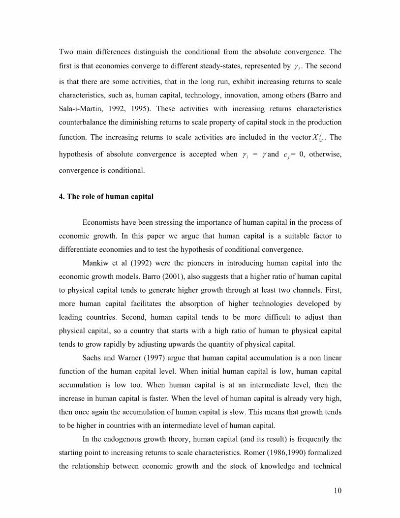
Economic activity in Brazil is concentrated mainly in the Southeast area as Table

1 shows. In 2000, the Southeast area accounted for about 57% of the Brazilian GDP and

its per capita income was almost three times higher than that of the Northeast.

Table 1. Brazil – Regional indicators of GDP and education

Source: IPEA((Institute of applied economic research)

Regional differences also apply when we focus on educational indicators. The

illiteracy rate (IR) in the Northeast shows that almost 23% of its population was not able

13

to read (or write) in 2003, while in the South and Southeast this rate was about 6%. The

Northeast area also records the lowest rate of school attainment across all Brazil. People

from the Northeast spend on average 4.7 years at school while in the South and Southeast

spend about 7 years at school.

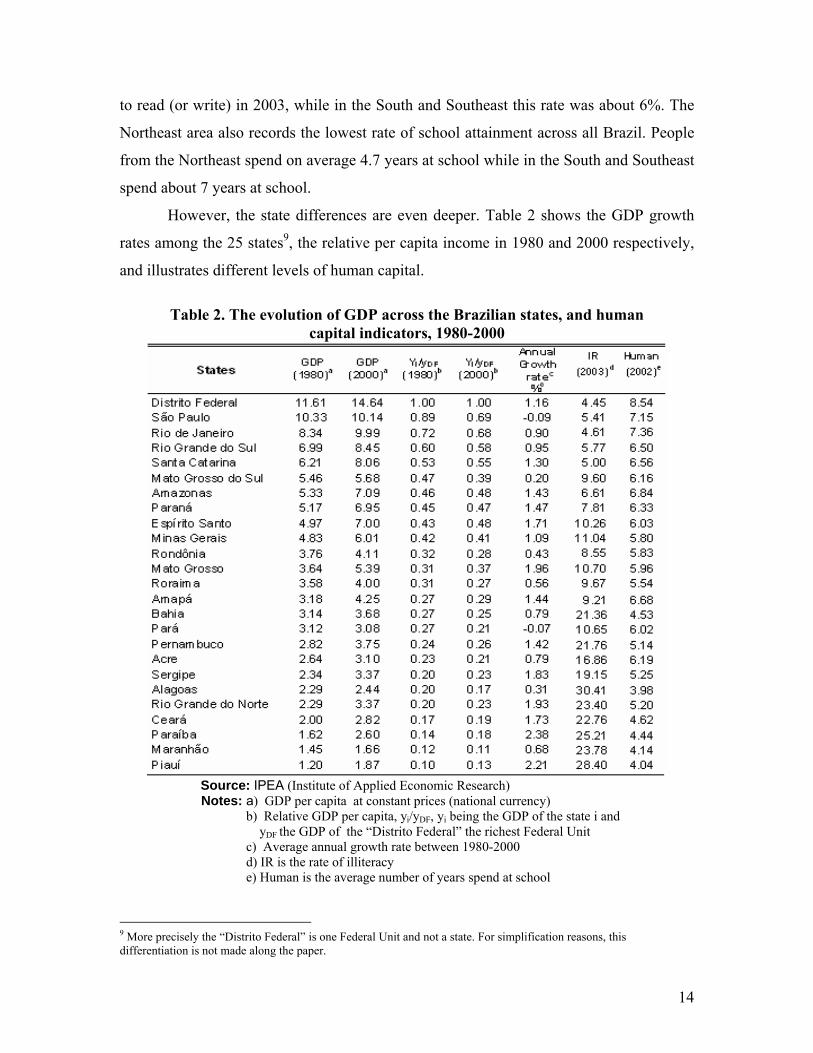
However, the state differences are even deeper. Table 2 shows the GDP growth

rates among the 25 states9, the relative per capita income in 1980 and 2000 respectively,

and illustrates different levels of human capital.

Table 2. The evolution of GDP across the Brazilian states, and human

capital indicators, 1980-2000

Source: IPEA (Institute of Applied Economic Research) Notes: a) GDP per capita at constant prices (national currency) b) Relative GDP per capita, yi/yDF, yi being the GDP of the state i and yDF the GDP of the “Distrito Federal” the richest Federal Unit c) Average annual growth rate between 1980-2000 d) IR is the rate of illiteracy e) Human is the average number of years spend at school

9 More precisely the “Distrito Federal” is one Federal Unit and not a state. For simplification reasons, this differentiation is not made along the paper.

14

The data from Table 2 shows, for example, that in 2000 the GDP of the state of

“Maranhão” was only 11% of that of the “Distrito Federal” and that only five states have

achieved half of the GDP of the “Distrito Federal”. Human capital, expressed by IR and

Human, also displays huge disparities across states. In 2003, the rate of illiteracy was

28.40% in the state of “Piauí” while in “São Paulo” was only 5%. In the state of “Ceará”

people spend about 4.62 years of their lives studying at school, versus 7.36 years in the

state of “Rio de Janeiro”.

After highlighting the differences among the Brazilian states, we shall try to

identify any tendency towards converge. From column 4, of Table 2, comparatively to

column 3 we can observe that some rich states (on the top of the table) reduced their

relative position in terms of per capita income and some poor states (on the bottom of the

table) improved their relative position. On the other hand, column 5 shows that some

poor regions (Piauí, Paraíba, Ceará) grew faster relatively to some rich states (São Paulo,

Rio de Janeiro, Rio Grande do Sul) over the period 1980-2000. This preliminary

observation can be taken as evidence of catching up and absolute convergence.

In a more formal way, the coefficient of variation can be used to measure σ-

convergence, indicating if asymmetries across economies are declining over time. Figure

1 plots the evolution of the coefficient of variation referred to GDP per capita of the

Brazilian states over the period 1980-2000.

Figure 1. σ-convergence among the states of Brazil 1980-2000

15

As it can be seen the dispersion of per capita income has been reduced over the whole

period, the reduction being more intensive in the beginning of the period. We can also

observe a period of divergence between 1986 and 1992 which coincides with the period

of hyper-inflation and general macroeconomic instability in Brazil. Ferreira (2000) has

also found σ-convergence among the Brazilian states over the period 1975-1995.

7. Absolute convergence

As we explained in section 4, the hypothesis of absolute convergence can be

tested by estimating equation (17)10 which relates the growth of per capita income to the

log of the initial level of the respective economy. Average annual growth rates in per

capita income, calculated every five years, are used to measure convergence among the

states of Brazil, over the period 1980-2000. Brazil (25 states) is also divided into two

sub-samples, the South/Southeast area with the 7 more developed states and the

Northeast area with the 9 less developed states. The scope of this division is to detect

different convergence processes across Brazil confirming, therefore, the convergence-

club hypothesis. The convergence equation has been estimated by the usual panel

estimation methods and the results are reported in Table 3.

As we can see, the pooled regressions give evidence of absolute convergence

which runs at very slow rates, 0.26% for Brazil, 0,56% for the South/Southeast and

0.72% for the Northeast areas. This result is consistent with the hypothesis that absolute

convergence occurs between economies with similar characteristics in terms of

institutions, policies, same language, free factor mobility, among others. We also note

that convergence is more robust when specific effects are introduced to control

differences in economic structures between the states. When state dummies are used

convergence is higher in all samples, 3.78% for Brazil, 1.39% for the South/Southeast

and 4.32% for the Northeast areas. The degree of explanation has increased significantly

except for the South/Southeast area. When specific effects are assumed to be random

10 This equation is the same as equation (1) of section 2.

16

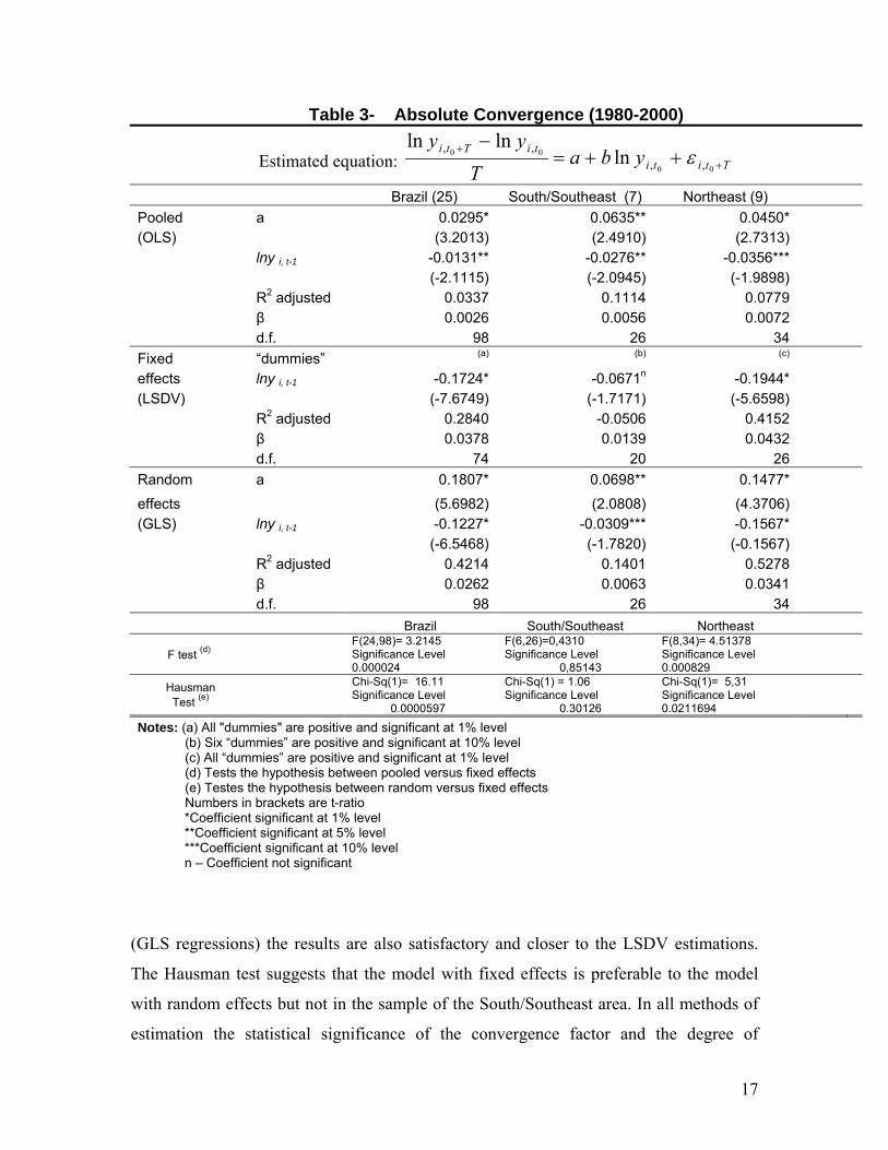
Table 3- Absolute Convergence (1980-2000)

Estimated equation: TtititiTti yba

Tyy

++ ++=

−00

00,,

,, lnlnln

ε

Brazil (25) South/Southeast (7) Northeast (9) Pooled a 0.0295* 0.0635** 0.0450*

(OLS) (3.2013) (2.4910) (2.7313) lny i, t-1 -0.0131** -0.0276** -0.0356***

(-2.1115) (-2.0945) (-1.9898) R2 adjusted 0.0337 0.1114 0.0779 β 0.0026 0.0056 0.0072 d.f. 98 26 34Fixed “dummies” (a) (b) (c)

effects lny i, t-1 -0.1724* -0.0671n -0.1944*

(LSDV) (-7.6749) (-1.7171) (-5.6598) R2 adjusted 0.2840 -0.0506 0.4152 β 0.0378 0.0139 0.0432 d.f. 74 20 26Random a 0.1807* 0.0698** 0.1477*

effects (5.6982) (2.0808) (4.3706)(GLS) lny i, t-1 -0.1227* -0.0309*** -0.1567*

(-6.5468) (-1.7820) (-0.1567) R2 adjusted 0.4214 0.1401 0.5278 β 0.0262 0.0063 0.0341 d.f. 98 26 34

Brazil South/Southeast Northeast

F test (d) F(24,98)= 3.2145 Significance Level 0.000024

F(6,26)=0,4310 Significance Level 0,85143

F(8,34)= 4.51378 Significance Level 0.000829

Hausman Test (e)

Chi-Sq(1)= 16.11 Significance Level 0.0000597

Chi-Sq(1) = 1.06 Significance Level 0.30126

Chi-Sq(1)= 5,31 Significance Level 0.0211694

Notes: (a) All "dummies" are positive and significant at 1% level (b) Six “dummies” are positive and significant at 10% level (c) All “dummies” are positive and significant at 1% level (d) Tests the hypothesis between pooled versus fixed effects (e) Testes the hypothesis between random versus fixed effects Numbers in brackets are t-ratio

*Coefficient significant at 1% level **Coefficient significant at 5% level ***Coefficient significant at 10% level n – Coefficient not significant

(GLS regressions) the results are also satisfactory and closer to the LSDV estimations.

The Hausman test suggests that the model with fixed effects is preferable to the model

with random effects but not in the sample of the South/Southeast area. In all methods of

estimation the statistical significance of the convergence factor and the degree of

17

explanation of the regressors in the South/Southeast area, are weak. These results are in

line with Ferreira (2000) and Barossi and Azonni (2003) who also found absolute

convergence for the Brazilian states.

The weak absolute convergence found in this section induces us to search for

conditional convergence, as the fixed effects estimations suggest. Human capital is

assumed to be the conditional factor to control properly structural differences between the

states of Brazil.

8. Convergence conditional to human capital

The previous section argues that the convergence process among the Brazilian

states can be better described when different equilibrium points are assumed for each

state. In other words, each state converges to his own steady-state and this is the essence

of conditional convergence. To control the different equilibrium points we use different

proxies for human capital, such as, the illiteracy rate (IR), the enrolment rate at the

secondary school (SEC) and average years of school attainment (SCHOOL) to express

the basic and intermediate levels of human capital qualifications. Additionally, the rate of

scientific publications (nº of articles per million of inhabitants, ART or nº of articles per

thousand of graduates, ARG11) is used to express differences in scientific production

reflecting higher levels of human capital, All these proxies are introduced separately into

the convergence equation, to avoid colinearity problems and to measure the individual

impact of each level of human capital on growth. The results of the panel estimations of

the conditional convergence equations using fixed effects are shown in Table 412.

As it can be seen, when the illiteracy rate is introduced into the convergence

equation its impact is negative as expected, revealing that the higher the rate of illiteracy

the lower is the growth of per capita income. Convergence among the Brazilian states

11 The number of graduate students (in the last semester of attainment of the graduate course) is provided by INEP (www.inep.gov.br). 12 Ferreira (2000) and Azzoni et al (2000) have introduced other variables in the convergence regression and found conditional convergence to human capital for the Brazilian states. However, their results are not directly comparable to ours since we have included different levels of human capital separately and the methodology used is also different.

18

Table 4- Conditional Convergence (1980-2000) - Fixed effects

Estimated equation: Ttitij

jtitiTti Xyba

Tyy

++ +++=

−000

00,,,

,, lnlnln

εψ

Brazil South/Southeast Northeast “dummies” * * lny i, t-1 -0.2218* -0.2174* -0.2209* (-10.6307) (-6.1292) (-6.2916)

IR IR -0.0739* -0.0724* -0.0520**Illiteracy rate (-5.6037) (-5.7824) (-2.0021)

R2 adjusted 0.4925 0.5992 0.4759 β 0.0502 0.0490 0.0499 d.f. 73 19 25 Test F(a)

Signif. Level F(24,97)=5.7404

0.0000 F(6,25)=5.4429

0.0010 F(6,25)=5.6320

0.0001 Hausman Test(b)

Signif. Level Chi-Sq(2)=15.7325

0.0003 Chi-Sq(2)=2.9983

0.2233 Chi-Sq(2)=4.4364

0.1088 “dummies” * lny i, t-1 -0.2123* -0.2359* -0.2339* (-9.9175) (-5.0165) (-7.0516) SEC SEC 0.0323* 0.0432* 0.0325*Enrolment (4.7944) (4.4678) (2.9118)Rate at R2 adjusted 0.4480 0.4607 0.5458secondary β 0.0477 0.0538 0.0532school d.f. 73 19 25 Test F(a)


0.0000 F(6,25)=4.1953

0.0047 F(6,25)=7.1419



0.0002 Chi-Sq(2)=3.1529

0.2067 Chi-Sq(2)=4.2841

0.11741 “dummies” * lny i, t-1 -0.2144* -0.2185* -0.2233* (-9.1098) (-4.5832) (-6.0977)

SCHOOL SCHOOL 0.0769* 0.1341* 0.0480***Average years (3.7537) (4.0357) (1.8070)Of schooling R2 adjusted 0.3916 0.4045 0.4621

β 0.0483 0.0493 0.0505 d.f. 73 19 25 Test F(a)


0.0000 F(6,25)=3.2490

0.0168 F(6,25)=5.3813

0.00022 Hausman Test (b)


0.0003 Chi-Sq(2)=3.1130

0.2108 Chi-Sq(2)=4.4613 /

0.10745 “dummies” * * * lny i, t-1 -0.1914* -0.2512* -0.2058* (-8.1127) (-6.4581) (-4.7684)

ART ART 0.0067** 0.0283* 0.0026n

scientific (2.1751) (5.9630) (0.4499)production R2 adjusted 0.3183 0.6148 0.3967

β 0.0425 0.0578 0.0461 d.f. 73 19 25 Test F(a)


0.0000 F(6,25)=7.2723

0.00014 F(6,25)=4.3730



0.0004 Chi-Sq(2)=2.9441

0.22944 Chi-Sq(2)=4.4676

0.10711

19

Table 4 (continued)

“dummies” * * *

lny i, t-1 -0.1878* -0.2184* -0.1918* (-6.4574) (-6.3880) (-4.2422)

ARG ARG 0.0070n 0.0292* -0.0006n

Scientific (1.5313) (6.0675) (-0.0897)Production R2 adjusted 0.2517 0.6235 0.3920

β 0.0416 0.0492 0.0426 d.f. 64 19 25 Test F(a)


0.0003 F(6,25)=6.7471

0.0002 F(6,25)=3.7424



0.0015 Chi-Sq(2)=2.9777

0.2256 Chi-Sq(2)=4.3911

0.11129 Notes: IR is the illiteracy rate of the population with age over 15 SEC is the percentage of young people with age between 15 and 17 that attended the secondary school or they had completed 8 years of schooling SCHOOL is the average number of school attainment of the population with age over 25 ART is the number of published papers in international journals per million of inhabitants ARG is the number of published papers in international journals per thousand of graduates (a) Tests the hypothesis between pooled versus fixed effects (b) Testes the hypothesis between random versus fixed effects Numbers in brackets are t-ratio *Coefficient significant at 1% level ** Coefficient significant at 5% level *** Coefficient significant at 10% level n – Coefficient not significant,

now runs at a higher annual rate, around 5% in all samples. The estimated equations are

more robust (comparing to the absolute convergence) in terms of the statistical

significance of the coefficients and the degree of explanation of the regressors. Therefore,

human capital in its lowest level controls satisfactorily the differences between the

Brazilian states. The convergence process is similar in all samples, not being able to

distinguish any differences between the most developed (South/Southeast) and the less

developed (Northeast) states.

The results are also satisfactory when the enrolment rate at the secondary school

is used to express basic levels of human capital. All coefficients have the predicted signs

and are highly significant, indicating that human capital stock at the secondary level is

relevant in explaining the convergence process among the Brazilian states. This variable

contributes positively to the increase in wealth in this country and this is shown in all

samples. Convergence runs at a similar annual rate of around 5.3% in the

South/Southeast and Northeast areas and it is somehow higher than the convergence

found by using the illiteracy rate. Once again, the convergence process is not

differentiated between these two subsets.

20

Convergence has been found to be similar in the three samples when the average

years of school attainment is used as proxy for intermediate levels of human capital,

running at 5% per year. The effect of this type of human capital stock on growth is

positive and higher than in the previous proxies of literacy levels, in all samples. An

interesting thing to note is that the marginal effect of this type of human capital is higher

in the sample of the more developed (South/Southeast) area. Every additional year in

education induces 0.13% increase in wealth in the South/Southeast area against only

0.05% in the Northeast. This level of Human capital is more efficient in the

South/Southeast area inducing higher growth. The same Human capital has a smaller

impact on growth in the Northeast area and its statistical significance is weak. It seems

that this intermediate level of human capital differentiates now the convergence process

between the South/Southeast and the Northeast areas. The Northeast area constituted by

less developed states has to improve farther the intermediate educational levels to achieve

higher growth.

The last proxy we use for human capital is the rate of scientific publications per

million of inhabitants (ART) or alternatively per thousand of graduates (ARG). These

variables attempt to capture higher levels of human capital related to scientific production

ability. Now the impact of this type of human capital differentiates clearly the

convergence process between the South/Southeast and Northeast areas. ART is highly

significant in the sample of the South/Southeast that comprises the more developed states

and it doesn’t have any significance in the Northeast sample, constituted by the less

developed states of Brazil. Convergence also runs at a higher rate in the South/Southeast

area, 5.7% against 4.6% in the Northeast area and the degree of explanation of the

regressors is much higher in the South/Southeast sample than in the others. The

alternative variable ARG has a similar behaviour not altering the conclusions derived

from ART. The rate of convergence, the marginal impact of human capital and the

robustness of the estimation are weak for the sample of Brazil relatively to the previous

estimations where intermediate levels of human capital were used.

The Arellano-Bond (1991) dynamic panel data estimation technique has also been

used to estimate the convergence equations taking care of the endogeneity problem of the

21

regressors, The obtained results were similar to Table 4, not contradicting the main

findings. For comparison, these results are reported in the Appendix.

Our evidence at this stage seems to suggest that intermediate levels of human

capital expressed mostly by SCHOOL explain better the convergence process in all

samples. Convergence is higher and the impact of this level of human capital stock on

growth stronger, especially in the South/Southeast zone. This is consistent with the Sachs

and Warner (1997) argument that growth tends to be higher in countries with an

intermediate level of human capital. On the other hand the differentiation in the

convergence process between the South/Southeast and Northeast areas lays on the use of

higher levels of human capital that have stronger effects in the former than in the latter.

Higher levels of human capital expressed by ART or ARG control better the differences

between the more developed states than the less developed states of Brazil. Higher levels

of human capital do not make a significant contribution to growth in the Northeast area.

This shows that the Northeast area has to improve primarily the basic and intermediate

levels of human capital before going to develop higher levels of education.

9. Main conclusions

In this paper we have analysed the convergence process across the Brazilian states

over the period 1980-2000. Our analysis has been focused on the issue of conditional

convergence considering various levels of human capital to control differences in

structures between the states of Brazil.

Initially we observed that the dispersion of per capita income among the Brazilian

states has been declining over time and this is evidence of σ-convergence. Absolute

convergence also found, but the estimations are not robust. On the other hand conditional

convergence on human capital boosts the results, reinforcing the convergence rate and

increasing the degree of explanation. In general, it can be assumed that convergence in

per capita income among the Brazilian states runs at approximately 5% per year when

differences in human capital are controlled for. This is higher than the standard 2% rate

stylized by Barro,

22

A farther finding in this study is that the intermediate levels of human capital

explain better the convergence process among the Brazilian states. When this type of

human capital is used convergence is higher and the marginal impact on growth

significantly stronger, improving the standards of living of the populations to a greater

extent. This is consistent with the idea that growth tends to be higher in countries (or

states) with an intermediate level of human capital.

The conditional convergence estimation approach on the other hand shows that

different levels of human capital have different responses to growth depending on the

sample used. Variables that represent higher levels of human capital affect more

efficiently the more developed than the less developed states in Brazil.

Generally our results suggest that the proposed human capital variables properly

control the differences in the steady-states across the Brazilian states and their influence

to growth is depending on the level of human capital they intent to represent. Therefore,

to optimally exploit resources, human capital improvements have to be progressive.

23

Appendix

Dynamic panel estimation (GMM:Arellano-Bond)

One criticism that is often made to the estimation of the convergence equations is

that, the conventional estimation methods used fail to account for the endogeneity of the

regressors. When explanatory variables are endogenous the regression estimates are

biased and inconsistent,

To account for endogeneity we estimate the convergence equation by using the

GMM estimation approach proposed by Arellano-Bond (1991) and first employed by

Caselli et al (1996). The growth equation is first differenced to eliminate the specific

effects and then all lags of the explanatory variables are used as instruments. The

dynamic estimated equation is, therefore

TtitititiTti Xybyy ++ ∆+∆+∆=−∆00000 ,,,,, lnln)5/)ln((ln εψ

The results of the estimation of this equation are shown in Table 5. The J-

specification statistic confirms in most cases the validity of the instruments used in the

estimation. The degree of explanation and the statistical significance of the regressors are

more robust (smaller standard errors). Generally, these new results validate the previous

findings of Table 4.The introduction of human capital reinforces the convergence process

showing the potential role of human capital to growth. The basic and intermediate levels

of human capital are those that better explain the convergence process across Brazil. The

higher levels of human capital have a stronger growth impact in the South/Southeast area.

All human capital levels are significant in the Northeast area but the growth impact of the

intermediate levels (SEC) is stronger.

24

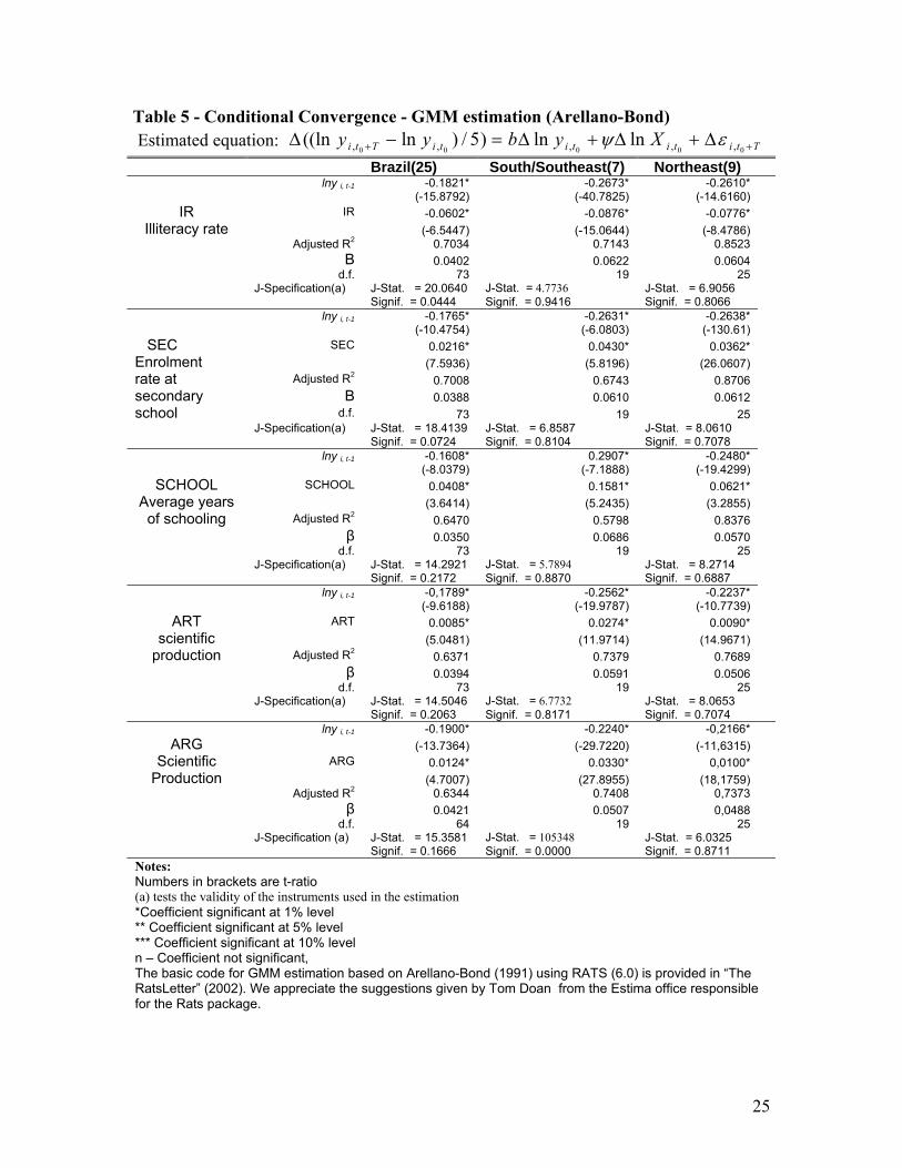
Table 5 - Conditional Convergence - GMM estimation (Arellano-Bond) Estimated equation: TtitititiTti Xybyy ++ ∆+∆+∆=−∆

00000 ,,,,, lnln)5/)ln((ln εψ Brazil(25) South/Southeast(7) Northeast(9) lny i, t-1 -0.1821* -0.2673* -0.2610* (-15.8792) (-40.7825) (-14.6160)

IR IR -0.0602* -0.0876* -0.0776*

Illiteracy rate (-6.5447) (-15.0644) (-8.4786) Adjusted R2 0.7034 0.7143 0.8523

Β 0.0402 0.0622 0.0604 d.f. 73 19 25 J-Specification(a) J-Stat. = 20.0640

Signif. = 0.0444 J-Stat. = 4.7736 Signif. = 0.9416

J-Stat. = 6.9056 Signif. = 0.8066

lny i, t-1 -0.1765* -0.2631* -0.2638* (-10.4754) (-6.0803) (-130.61) SEC SEC 0.0216* 0.0430* 0.0362*

Enrolment (7.5936) (5.8196) (26.0607) rate at Adjusted R2 0.7008 0.6743 0.8706 secondary Β 0.0388 0.0610 0.0612 school d.f. 73 19 25 J-Specification(a) J-Stat. = 18.4139


J-Stat. = 8.0610 Signif. = 0.7078

lny i, t-1 -0.1608* 0.2907* -0.2480* (-8.0379) (-7.1888) (-19.4299)

SCHOOL SCHOOL 0.0408* 0.1581* 0.0621*

Average years (3.6414) (5.2435) (3.2855) of schooling Adjusted R2 0.6470 0.5798 0.8376

β 0.0350 0.0686 0.0570 d.f. 73 19 25 J-Specification(a) J-Stat. = 14.2921


J-Stat. = 8.2714 Signif. = 0.6887

lny i, t-1 -0,1789* -0.2562* -0.2237* (-9.6188) (-19.9787) (-10.7739)

ART ART 0.0085* 0.0274* 0.0090*

scientific (5.0481) (11.9714) (14.9671) production Adjusted R2 0.6371 0.7379 0.7689

β 0.0394 0.0591 0.0506 d.f. 73 19 25 J-Specification(a) J-Stat. = 14.5046


J-Stat. = 8.0653 Signif. = 0.7074

lny i, t-1 -0.1900* -0.2240* -0,2166* ARG (-13.7364) (-29.7220) (-11,6315)

Scientific ARG 0.0124* 0.0330* 0,0100*

Production (4.7007) (27.8955) (18,1759) Adjusted R2 0.6344 0.7408 0,7373

β 0.0421 0.0507 0,0488 d.f. 64 19 25 J-Specification (a) J-Stat. = 15.3581

Signif. = 0.1666 J-Stat. = 105348 Signif. = 0.0000

J-Stat. = 6.0325 Signif. = 0.8711

Notes: Numbers in brackets are t-ratio (a) tests the validity of the instruments used in the estimation *Coefficient significant at 1% level ** Coefficient significant at 5% level *** Coefficient significant at 10% level n – Coefficient not significant, The basic code for GMM estimation based on Arellano-Bond (1991) using RATS (6.0) is provided in “The RatsLetter” (2002). We appreciate the suggestions given by Tom Doan from the Estima office responsible for the Rats package.

25

References

Arellano, M., Bond, S., (1991), Some Tests of Specification for Panel Data: Monte Carlo Evidence and an Application to Employment Equations, Review of Economic Studies, 58, 277-297. Azzoni, C., Menezes, N., Menezes, T., Silveira Neto, R., (2000), Geography and Income Convergence and Among Brazilian States, Interamerican Development Bank, Research Network Working Papers; R-395. Barro, R., (1991), Economic Growth in a Cross Section of Countries, Quarterly Journal of Economics, 106, 2, 407-43. Barro, R., (2001), Human Capital: Growth, History and Policy – A Session to Honour Stanley Engerman, Human Capital and Growth, American Economic Review, 91, 2, 12-17. Barro, R., Sala-i-Martin, X., (1992), Convergence, Journal of Political Economy, 100, 2, 223-251. Barro, R., Sala-i-Martin, X., (1995), Economic Growth, McGraw Hill, New York. Barro, R., Sala-i-Martin, X., (1997), Technological Diffusion, Convergence and Growth, Journal of Economic Growth, 2, 1-27. Barossi Fo, M., Azzoni, C., (2003), A Time Series Analysis of Regional Income Convergence in Brazil, Artigos Nemesis, http://www,nemesis,org,br/ Bernardes, A., Albuquerque, E., (2003), Cross-over, Thresholds, and Interaction Between Science and Technology: lessons for less-developed countries, Research Policy 32, 865-885. Ferreira, A., (2000), Convergence in Brazil: Recent trends and long-run prospects, Applied Economics, 32, 479-489. Galor, O., (1996), Convergence? Inference from Theoretical Models, The Economic Journal, 106, 1056-1069. Islam, N., (1995), Growth Empirics: A panel data approach, The Quarterly Journal of Economics, 110, 4, 1127-1170. Lucas, R., (1988), On the Mechanics of Economic Development, Journal of Monetary Economics, 22, 1, 3-42.

26

Mankiw G., Romer D., Weil D., (1992), A Contribution to the Empirics of Economic Growth, Quarterly Journal of Economics, 107, 2, 404-437. Patel, P., Pavitt, K., (1995), Patterns of Technological Activity: their measurement and interpretation, In: Stoneman, P., (Ed.), Handbook of the Economics of Innovation and Technological Change, Blackwell, Oxford. Romer, P., (1986), Increasing Returns and Long Run Growth, Journal of Political Economy, 94, 5, 1002-1037. Romer, P., (1990), Endogenous Technological Change, Journal of Political Economy, 98, S71-S102. Sachs, J., Warner, A., (1997), Fundamental Sources of Long Run Growth, American Economic Review, 87, 2, 184-188. Sala-i-Martin, X., (1996), The Classical Approach to Convergence Analysis, The Economic Journal, 106, 1019-1036. Solow, R., (1956), A Contribution to the Theory of Economic Growth, Quarterly Journal of Economics, LXX, 65-94. Temple, J., (1999), The New Growth Evidence, Journal of Economic Literature, XXXVII, 112-156. The RatsLetter, Volume 15, nº 2, November 2002, Evanston, IL, USA.

27

List of the Discussion Papers published by CEUNEUROP

Year 2000 Alfredo Marques - Elias Soukiazis (2000). “Per capita income convergence across countries and across regions in the European Union. Some new evidence”. Discussion Paper Nº1, January. Elias Soukiazis (2000). “What have we learnt about convergence in Europe? Some theoretical and empirical considerations”. Discussion Paper Nº2, March. Elias Soukiazis (2000). “ Are living standards converging in the EU? Empirical evidence from time series analysis”. Discussion Paper Nº3, March. Elias Soukiazis (2000). “Productivity convergence in the EU. Evidence from cross-section and time-series analyses”. Discussion Paper Nº4, March. Rogério Leitão (2000). “ A jurisdicionalização da política de defesa do sector têxtil da economia portuguesa no seio da Comunidade Europeia: ambiguidades e contradições”. Discussion Paper Nº5, July. Pedro Cerqueira (2000). “ Assimetria de choques entre Portugal e a União Europeia”. Discussion Paper Nº6, December.

Year 2001 Helena Marques (2001). “A Nova Geografia Económica na Perspectiva de Krugman: Uma Aplicação às Regiões Europeias”. Discussion Paper Nº7, January. Isabel Marques (2001). “Fundamentos Teóricos da Política Industrial Europeia”. Discussion Paper Nº8, March. Sara Rute Sousa (2001). “O Alargamento da União Europeia aos Países da Europa Central e Oriental: Um Desafio para a Política Regional Comunitária”. Discussion Paper Nº9, May.

Year 2002 Elias Soukiazis e Vitor Martinho (2002). “Polarização versus Aglomeração: Fenómenos iguais, Mecanismos diferentes”. Discussion Paper Nº10, February.

28

Alfredo Marques (2002). “Crescimento, Produtividade e Competitividade. Problemas de desempenho da economia Portuguesa” . Discussion Paper Nº 11, April. Elias Soukiazis (2002). “Some perspectives on the new enlargement and the convergence process in Europe”. Discussion Paper Nº 12, September. Vitor Martinho (2002). “ O Processo de Aglomeração nas Regiões Portuguesas”. Discussion Paper, Nº 13, November.

Year 2003 Elias Soukiazis (2003). “Regional convergence in Portugal”. Discussion Paper, Nº 14, May. Elias Soukiazis and Vítor Castro (2003). “The Impact of the Maastricht Criteria and the Stability Pact on Growth and Unemployment in Europe” Discussion Paper, Nº 15, July. Stuart Holland (2003a). “Financial Instruments and European Recovery – Current Realities and Implications for the New European Constitution”. Discussion Paper, Nº 16, July. Stuart Holland (2003b). “How to Decide on Europe - The Proposal for an Enabling Majority Voting Procedure in the New European Constitution”. Discussion Paper, Nº 17, July. Elias R. Silva (2003). “Análise Estrutural da Indústria Transformadora de Metais não Ferrosos Portuguesa”, Discussion Paper, Nº 18, September. Catarina Cardoso and Elias Soukiazis (2003). “What can Portugal learn from Ireland? An empirical approach searching for the sources of growth”, Discussion Paper, Nº 19, October. Luis Peres Lopes (2003). “Border Effect and Effective Transport Cost”. Discussion Paper, Nº 20, November. Alfredo Marques (2003). “A política industrial face às regras de concorrência na União Europeia: A questão da promoção de sectores específicos” Discussion Paper, Nº 21, December.

Year 2004 Pedro André Cerqueira (2004). “How Pervasive is the World Business Cycle?” Discussion Paper, Nº 22, April.

29

Helena Marques and Hugh Metcalf (2004). “Immigration of skilled workers from the new EU members: Who stands to lose?” Discussion Paper, Nº 23, April.

Elias Soukiazis and Vítor Castro (2004). “How the Maastricht rules affected the convergence process in the European Union. A panel data analysis”. Discussion Paper, Nº 24, May.

Elias Soukiazis and Micaela Antunes (2004). “The evolution of real disparities in Portugal among the Nuts III regions. An empirical analysis based on the convergence approach”. Discussion Paper, Nº 25, June. Catarina Cardoso and Elias Soukiazis (2004). “What can Portugal learn from Ireland and to a less extent from Greece? A comparative analysis searching for the sources of growth”. Discussion Paper, Nº 26, July. Sara Riscado (2004), “Fusões e Aquisições na perspectiva internacional: consequências económicas e implicações para as regras de concorrência”. Documento de trabalho, Nº 27, Outubro.

Year 2005 Micaela Antunes and Elias Soukiazis (2005). “Two speed regional convergence in Portugal and the importance of structural funds on growth”. Discussion Paper, Nº 28, February. Sara Proença and Elias Soukiazis (2005). “Demand for tourism in Portugal. A panel data approach”. Discussion Paper, Nº 29, February. Vitor João Pereira Martinho (2005). “Análise dos Efeitos Espaciais na Produtividade Sectorial entre as Regiões Portuguesas”. Discussion Paper, Nº 30, Abril. Tânia Constâncio(2005). “Efeitos dinâmicos de integração de Portugal na UE” Discussion Paper, Nº 31, Março. Catarina Cardoso and Elias Soukiazis (2005). “Explaining the Uneven Economic Performance of the Cohesion Countries. An Export-led Growth Approach.” Discussion Paper, Nº 32, April. Alfredo Marques e Ana Abrunhosa (2005). “Do Modelo Linear de Inovação à Abordagem Sistémica - Aspectos Teóricos e de Política Económica” Documento de trabalho, Nº 33, Junho. Sara Proença and Elias Soukiazis (2005). “Tourism as an alternative source of regional growth in Portugal”, Discussion Paper, Nº 34, September.

30

Túlio Cravo and Elias Soukiazis (20006). “Human capital as a conditioning factor to the convergence process among the Brazilian States”, Discussion Paper, Nº 35, February.

31

Centro de Estudos da União Europeia (CEUNEUROP) Faculdade ...

Documents

Transcript of Centro de Estudos da União Europeia (CEUNEUROP) Faculdade ...