Centrifuge Modeling of Lateral-Axial Oblique Loading on

Buried Pipelines in Cohesionless Soil

by

Gabrielle Marcotte

A thesis submitted to the Faculty of Graduate and Postdoctoral Affairs in

partial fulfillment of the requirements for the degree of

Master of Applied Science

in

The Department of Civil and Environmental Engineering

Carleton University

Ottawa, Ontario

© 2017, Gabrielle Marcotte

i

Abstract

Pipelines may be subject to oblique loading conditions due to relative ground motion

associated with geohazards including ground subsidence, slope movement/failure, frost heave

and fault movement. Conventional guidelines for engineering stress analysis of pipe/soil

interaction employ a series of orthogonal, independent springs, within structural based finite

element modelling procedures, to represent soil reaction loads. This formulation does not

properly account for coupled load effects during oblique pipe/soil interaction events as it is

unable to account for the complex relationship between the soil and pipeline or the load effects

induced by loading in multiple directions.

A series of reduced scale physical tests to investigate oblique load effects, in the lateral-axial

plane, on a buried pipe in cohesionless soil were conducted using a rigid, 46 mm diameter pipe.

The pipe was buried at two burial depths, H/D of 2 and 4, and was tested at five different angles

between 0° (pure axial) and 90° (pure lateral). The shallow buried pipe modelled a prototype 304

mm diameter pipeline, and a prototype 609.5 mm diameter pipeline for the deeper burial depth.

Failure surfaces for the yield load compared favourably with previous physical tests and

numerical simulations of oblique loading events. In addition, the mobilization distance to yield

were comparable with previous reduced-scale tests but the results were more consistent with the

ALA guidelines, which was attributed to the experimental procedures and use of acoustic foam

to moderate spurious boundary conditions effects on the measured response.

ii

Acknowledgements

I would like first to like to thank Professors Shawn Kenny and Siva Sivathayalan for all of

their help during this research. Their guidance and recommendations have helped me through the

long research and writing process.

I also would not have been able to complete this research without the support and

understanding of the staff of C-Core especially Mr. Gerry Piercy, and Mr. Karl Kuehnemund

who helped me daily in the lab with set-up, testing, and advice and Mr. Karl Tuff who helped me

with all of the electronics required during testing. Without the team at C-Core, their experience,

and their centrifuge, this research would not have been possible.

I would also like to thank my friends and family, especially Murray and Oliver, who have

encouraged me and provided emotional support during my research and the long writing process.

iii

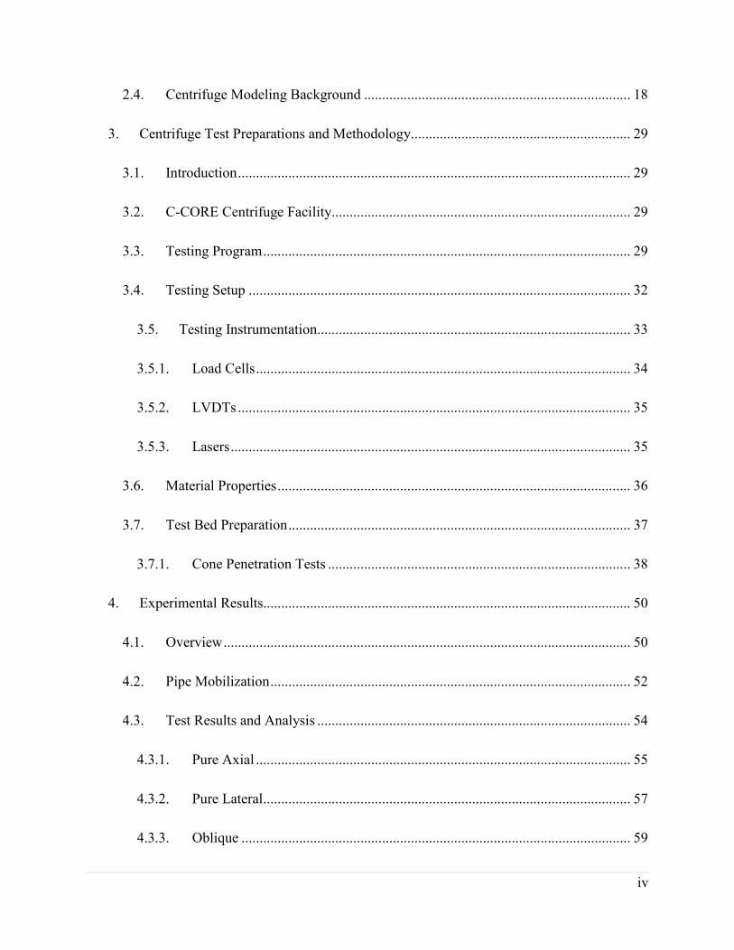
Table of Contents

Abstract ...................................................................................................................................... i

Acknowledgements ................................................................................................................... ii

List of Figures .......................................................................................................................... vi

List of Equations ....................................................................................................................... x

List of Tables ........................................................................................................................... xi

List of Abbreviations and Symbols......................................................................................... xii

1. Introduction ...................................................................................................................... 1

1.1. Background ............................................................................................................... 1

1.2. Problem Statement .................................................................................................... 2

1.3. Objective ................................................................................................................... 3

1.4. Outline of Thesis ....................................................................................................... 4

2. Literature Review ............................................................................................................. 6

2.1. Introduction ............................................................................................................... 6

2.2. Current Guidelines .................................................................................................... 6

2.3. Pipe/soil Interaction .................................................................................................. 8

2.3.1. Axial Pipe/Soil Interaction ................................................................................ 9

2.3.2. Lateral Pipe/Soil Interaction ............................................................................ 12

2.3.3. Vertical Pipe/Soil Interaction .......................................................................... 14

2.3.4. Axial-Lateral Pipe/Soil Interaction .................................................................. 16

iv

2.4. Centrifuge Modeling Background .......................................................................... 18

3. Centrifuge Test Preparations and Methodology............................................................. 29

3.1. Introduction ............................................................................................................. 29

3.2. C-CORE Centrifuge Facility................................................................................... 29

3.3. Testing Program ...................................................................................................... 29

3.4. Testing Setup .......................................................................................................... 32

3.5. Testing Instrumentation....................................................................................... 33

3.5.1. Load Cells ........................................................................................................ 34

3.5.2. LVDTs ............................................................................................................. 35

3.5.3. Lasers ............................................................................................................... 35

3.6. Material Properties .................................................................................................. 36

3.7. Test Bed Preparation ............................................................................................... 37

3.7.1. Cone Penetration Tests .................................................................................... 38

4. Experimental Results...................................................................................................... 50

4.1. Overview ................................................................................................................. 50

4.2. Pipe Mobilization .................................................................................................... 52

4.3. Test Results and Analysis ....................................................................................... 54

4.3.1. Pure Axial ........................................................................................................ 55

4.3.2. Pure Lateral ...................................................................................................... 57

4.3.3. Oblique ............................................................................................................ 59

v

4.3.4. Uplift ................................................................................................................ 62

5. Summary and Conclusions ............................................................................................. 85

6. Bibliography ................................................................................................................... 90

Appendix A – Soil Properties ................................................................................................. 99

Appendix B. - Instrument Calibration ................................................................................ 102

Appendix C. – Raw Test Data ............................................................................................ 106

Appendix D. – Test Scans .................................................................................................. 109

Appendix E. – Geo-Ottawa 2017 Paper ............................................................................. 120

vi

List of Figures

Figure 2-1 – Current Pipeline Model Approach (from Kenny and Jukes, 2015) ......................... 21

Figure 2-2 - Common measurement for buried pipeline including pipe diameter (D), cover depth

(c), burial depth (H), and embedment depth (h). ................................................................. 21

Figure 2-3- Lateral bearing capacity fit curve (Honegger and Nyman, 2004) ............................. 22

Figure 2-4- Lateral bearing force comparison for loose sands (a), dense sand (b), and pipe

diameters (c) (From Guo and Stolle, 2005) ......................................................................... 23

Figure 2-5- Downward bearing capacity factors (Meyerhof. 1995) ............................................ 24

Figure 2-6 - Uplift bearing factor for horizontal anchors in sand (Merifield and Sloan, 2006) ... 25

Figure 2-7 - Oblique pipe/soil interaction in loose sand (a) lateral loads, (b) axial loads (Hsu et

al. 2001) ............................................................................................................................... 25

Figure 2-8 - Oblique pipe/soil interaction in dense sand (a) lateral loads, (b) axial loads (Hsu et

al. 2001) ............................................................................................................................... 26

Figure 2-9 Lateral-Axial oblique loading failure envelope for non-cohesive soil with heavy pipe

configuration at an embedment ratio H/D=2 and interface friction factor of 0.5 (from

Kenny and Jukes, 20015) .................................................................................................... 27

Figure 2-10 Lateral- axial oblique loading failure envelope for cohesive soil (from Kenny and

Jukes, 2015) ......................................................................................................................... 28

Figure 3-1 – Schematic diagram of shallow and deep pipe embedment depth ............................ 41

Figure 3-2- Pipe Set-up within Strongbox (Debnath, 2016) ......................................................... 41

Figure 3-3- Pipe assembly (1) including biaxial load cell (2, 3), stanchions (4, 5), dog bone (6),

and back bracket (7). ........................................................................................................... 42

vii

Figure 3-4- Major elements of the centrifuge test apparatus („payload‟) including dog bone (6),

ball race (7, 8), LVDT (9), guiding plate (10), motorized carriage (11), laser (12), and cone

(13). ..................................................................................................................................... 42

Figure 3-5 – Pipe assembly (1) in strongbox after bedding layer including back bracket (7),

acoustic foam (14), and laser target (15). ............................................................................ 43

Figure 3-6- Load cell configuration, based on Stroud (from Debnath, 2016) .............................. 43

Figure 3-7- Load cell dimensions and schematic used for lateral load (from Daiyan, 2011) ....... 44

Figure 3-8- Load cell calibration apparatus used for lateral and axial loading ............................ 44

Figure 3-9- Crushable Acoustic Foam after Test 8, 20°, H/D=4D ............................................... 45

Figure 3-10- Sieve analysis results for sand used in testing ......................................................... 45

Figure 3-11 Simplified direct shear testing apparatus .................................................................. 46

Figure 3-12- Cone penetration tests results for shallow burial depth tests (H/D=2) .................... 47

Figure 3-13 - Cone penetration test results for deep burial depth tests (H/D=4) .......................... 48

Figure 3-14- CPT test results normalized to an acceleration of 1g............................................... 49

Figure 4-1 – Pipe orientation of shallow tests (Test 1 – 6, H/D=2) .............................................. 65

Figure 4-2 – Pipe orientation of deep tests (Tests 7-10, H/D=4) .................................................. 65

Figure 4-3 – Bending of the double dog-bone set-up before and after Test 10 (H/D=4, 30°). .... 66

Figure 4-4 - Load cell A after model pipe was pulled out from between stanchions (Test 9, 90°,

H/D=4) ................................................................................................................................. 67

Figure 4-5 - Motor seal failure after final test (Test 10, 30°, H/D=4) .......................................... 67

Figure 4-6 – Laser displacement as measured on the dog bone and actuator as a function of true

time (Test 4, 90°, H/D=2, no foam) ................................................................................... 68

viii

Figure 4-7 - Laser displacement as measured on the dog bone and actuator as a function of true

time (Test 10, 30°, H/D=4) .................................................................................................. 69

Figure 4-8 – Schematic of idealized pipeline lag during mobilization ......................................... 70

Figure 4-9 – Lateral Loads (normalized) as a function of corrected pipe movement (shallow

tests) ..................................................................................................................................... 71

Figure 4-10 - Normalize axial loads as a function of corrected pipe movement (deep tests) ....... 72

Figure 4-11 - Schematic illustration of peak load determination ( Pike et al. 2011, from Debnath,

2016) .................................................................................................................................... 73

Figure 4-12 – Results of pure axial tests as a function of pipe diameter (Test 2- H/D=2, Test 7-

H/D=4) ................................................................................................................................. 74

Figure 4-13 - Comparison of axial test results to existing data (variation to Kenny et al., 2015) 75

Figure 4-14 – Results of the pure lateral tests as a function of pipe mobilization (Test 2- H/D=2

–no foam, Test 3 – H/D=2 – foam, Test 9 –H/D=4) ........................................................... 76

Figure 4-15 - Comparison of lateral test results in loose sands (variation on Kenny et al., 2015) 77

Figure 4-16 - Normalized axial load as a function of pipe displacement for oblique tests (50° -

H/D=2, 70° -H/D =2, 20° - H/D=4, 30° - H/D=4) .............................................................. 78

Figure 4-17 – Normalized lateral load as a function of the true pipe displacement for oblique

tests (50° -H/D=2, 70° -H/D =2, 20° - H/D=4, 30° - H/D=4) ............................................ 79

Figure 4-18 - Comparison of axial and lateral load results (variation on Kenny et al., 2015) ..... 80

Figure 4-19 – Test 5 (20°, H/D=2) post-test scan ......................................................................... 81

Figure 4-20 - Normalized lateral load as a function of pipe displacement (Test 6, 70°, H/D=2) 82

Figure 4-21 - Normalized axial loads as a function of pipe displacement (Test 6, 70°, H/D=2) 82

ix

Figure 4-22 – Uplift displacement of leading and trailing edge of dogbone (Test 4, 90°, H/D=2)

............................................................................................................................................. 83

Figure 4-23 - Soil Settlement as a function of time for Test 3, 5, 6, 7, 8, 9, and 10. .................... 84

Figure A-1 - Shear test results of silica sand used in test………………………..........................99

Figure A-2 - Normal stress (kPa) as a function of shear stress (kPa)………………………….100

Figure B-1 - LVDT 3031 calibration………………………………………………………...…104

Figure B-2 - LVDT 5080 calibration………………………………………………………...…104

Figure C-1 -Unprocessed lateral load (N) as a function of true pipe displacement (mm) for all

ten tests………..………………………………………………………………………….106

Figure C-2 - Unprocessed axial load (N) as a function of true pipe displacement (mm) for all ten

tests……………………………………………………………………..………………..107

Figure D-1 - Post-test scan Test 1 (50°, H/D=2, 6.25g)………………………………………109

Figure D-2 - Post-test scan Test 2 (0°, H/D=2, 6.25g)………………..………………………110

Figure D-3 - Post-test scan Test 3 (90°, H/D=2, no foam, 6.25g) without dogbone and with

dogbone…………..………………………………………………………………………111

Figure D-4 - Post-test scan of Test 4 (90°, H/D=2, with foam, 6.5g)………………..…………112

Figure D- 1 – Post-test scan of Test 5 (20°, H/D=2, 6.5g)………………………………..……113

Figure D- 2 – Post-test scan of Test 6 (70°, H/D=4, 6.5g)……………………………………..114

Figure D- 7 – Pre-test (right) and post-test (left) scans for Test 7 (0°, H/D=4, 13.25g)……….115

Figure D- 8 – Pre-test (right) and Post-test (left) scans of Test 8 (20°, H/D=4, 13.25g)…….…116

Figure D- 9 – Pre-test (right) and Post-test (left) scans of test 9 (90°, H/D=4, 13.25g)………..117

Figure D- 10 – Pre-test (right) and Post-test scan of test 10 (30°, H/D=4, 13.25g)……………118

x

List of Equations

Equation 2-1 .............................................................................................................................. 7

Equation 2-2 .............................................................................................................................. 9

Equation 2-3 .............................................................................................................................. 9

Equation 2-4 ............................................................................................................................ 10

Equation 2-5 ............................................................................................................................ 11

Equation 2-6 ............................................................................................................................ 11

Equation 2-7 ............................................................................................................................ 12

Equation 2-8 ............................................................................................................................ 13

Equation 2-9 ............................................................................................................................ 14

Equation 2-10 .......................................................................................................................... 15

Equation 2-11 .......................................................................................................................... 17

Equation 4-1 ............................................................................................................................ 52

Equation 4-2 ............................................................................................................................ 53

Equation 4-3 ............................................................................................................................ 54

xi

List of Tables

Table 2-1- Friction factor based on pipe coating, (ALA, 2005) ............................................. 20

Table 2-2- Common Scaling Relationships (from Taylor, 1995) ........................................... 20

Table 3-1 - Centrifuge strongbox and pipe model parameters ............................................... 40

Table 3-2 - Mobilization Angle and Density of Tests ............................................................ 40

Table 4-1 – Peak lateral load results and corresponding mobilization ................................... 64

Table 4-2 - Peak axial and lateral loads - oblique tests ........................................................... 64

Table

xii

List of Abbreviations and Symbols

B projected width of contact area

c cohesion of soil

cu undrained shear strength of soil

C depth of soil to the top of the pipe or cover depth

D external pipe diameter

Dr relative density

Dref reference diameter

E soil elastic modulus

ƒ friction factor of pipe

g gravitational acceleration

h depth of soil to the bottom of the pipe or embedment depth

H soil depth to centerline of pipe or springline cover depth

Ko coefficient of lateral earth pressure at rest

Ka coefficient of active lateral earth pressure

L pipe length

N gravitational acceleration factor

Nch, Nqh lateral interaction (bearing capacity) factors for cohesive and frictional effects

Ncv, Nqv vertical interaction (bearing capacity) factors for cohesive and frictional effects

Nqh(90) lateral interaction factor for pure lateral pipe/soil interaction

Nt axial interaction factor

Nc, Nq, Nγ bearing capacity factors for horizontal strip footings, vertically loaded down

p mean effective stress

po atmospheric (reference) pressure

q deviatoric stress

T, P, Q soil forces applied to unit length of pipe in axial, lateral and vertical direction

Tu, Pu, Qu ultimate soil forces applied to unit length of pipeline in axial, lateral and vertical

direction

t pipe wall thickness

Wp pipe self-weight

x, y, z relative pipe/soil displacement in axial, lateral, and vertical directions

xu, yu, zu ultimate relative pipe/soil displacement in axial, lateral, and vertical directions

Xu, Yu ratio of ultimate relative pipe/soil displacement in axial, and lateral directions over

pipe diameter

α lateral-vertical oblique angle of movement

γ‟ effective unit weight of soil

γd dry unit weight of soil

γd,min minimum dry unit weight of soil

δ interface friction factor of pipe and soil

θ axial-lateral oblique angle of movement

μ pipe/soil interface coefficient

ρ density of soil

ϕ‟ internal friction angle of soil

ψ dilation angle of soil

1

1. Introduction

1.1. Background

Pipelines are one of the most effective methods to transport liquids and gases over long

distances (NRCan, 2014). Across Canada, there is an estimated 852,000 km of energy

transmission pipelines. To minimize the effect of loads and potential damage caused by external

influences, from natural (e.g. wind, snow) and anthropogenic (e.g. third-party interference)

events, the majority of pipelines are buried.

Buried pipelines, however, can be subjected to large deformations and loads due to

geohazards (e.g. subsidence, liquefaction, unstable slopes, and freeze/thaw settlement) that can

damage the pipeline. Damaged pipelines may not be able to meet the operational and

serviceability requirements as mandated by codes and standards (e.g. Canadian Standard Z662)

or company specific thresholds (e.g. business or service risk).

Current engineering practices (e.g. ALA, 2005) used to analyze pipe/soil interaction events

are based on idealized structural models that have inherent bias and uncertainty. A better

understanding of the complex relationship between the pipeline and the surrounding soil needs to

be achieved. This improved understanding is required to help ensure that design guidelines and

maintenance requirements are economical and effective while taking safety into account.

Additional research will allow for higher confidence levels in the estimated lifespans for new and

ageing pipelines and will benefit all stakeholders including consultants, operators, regulators and

the public.

2

1.2. Problem Statement

Current design guidelines (e.g. ALA, 2005) are used as the technical basis to develop

structural based numerical modelling procedures simulating pipe/soil interaction events. The

models can then be used to analyze the soil loads imposed on the buried pipeline during

differential ground movement events as well as the pipeline stress and deformation experienced

during the event.

The traditional modeling approach is generally based on a Winkler-type beam/spring

foundation model with several underlying assumptions. The pipeline is idealized as a structural

element based on Euler or Timoshenko beam theory with additional variables to account for the

effects of internal pressure and thermal expansion. The continuum soil response is modelled

using a discrete series of distributed spring elements along the pipeline‟s longitudinal axis. For

three-dimensional analysis, three springs are placed along three mutually perpendicular axes

relative to the pipe cross-section. For this research, the three axes are stated as axial (i.e.

longitudinal), lateral (e.g. transverse horizontal), and vertical directions (e.g. transverse vertical).

Each soil spring element is uncoupled and acts independently. Generally, bilinear or hyperbolic

functions are used to determine the relationship between the soil yield load and the yield

displacement.

Previous studies have been conducted to determine if these assumptions are accurate and to

determine the soil yield load, mobilization distance to yield, and the soil failure mechanisms

during soil-pipeline displacement events (e.g. Hsu, 2001; Phillips et al, 2004; Debnath et al.

2016; Daiyan et al. 2010, 2011). These studies include theoretical studies, numerical studies, and

full-scale and reduce scaled experiments. It has been confirmed in these studies that although

uncoupled soil springs are easier to model, they do not always provide accurate results when

3

compared with full-scale or reduced-scale physical models and numerical continuum simulation

models are compared. The impact of pipeline weight, the interface conditions, burial depths, and

soil properties can also affect the results of the pipe/soil interaction models.

Completing additional physical models to confirm the scaling laws and soil behaviour can

reduce the limitations and uncertainty of the existing models. Due to the cost and time required

to complete full-scale model tests, this thesis will use reduced-scale centrifuge tests to confirm

the previously stated assumptions.

1.3. Objective

The main objective of this thesis is to improve the knowledge on soil load coupling effects

during pipe/soil interaction events for a rigid pipe translating within the axial-lateral plane

through loose cohesionless soil.

The main outcome of these tests is a new dataset for oblique axial-lateral pipe/soil interaction

events that can be compared with and augment existing datasets. Based on the dataset the yield

load, mobilization distance to yield, oblique yield load-displacement failure envelope and failure

mechanisms can be compared with previous studies that included reduced scale centrifuge

modelling, full-scale modelling, and numerical simulation. The data can be used to compare

results from other physical tests, as well as the calibration and verification of improved structural

based numerical modelling procedures addressing oblique load coupling effects on buried

pipelines. This integrated knowledge base can be used to inform current engineering practice and

may be used to advance engineering guidelines and best practice for structural based finite

element modelling of oblique pipe/soil interaction events.

4

1.4. Outline of Thesis

This thesis is separated into six chapters and five Appendices.

Chapter 1 provides an introduction to the thesis including background, problem statement and

research objectives.

Chapter 2 presents the literature review that covers the existing guidelines and previous research

including physical models, numerical models and mathematical models. This section will also

discuss previous pipe/soil interaction research and the principals of centrifuge modelling.

Chapter 3 discusses the centrifuge modelling conducted for this thesis. This will include the test

setup, apparatus, soil properties, testing instrumentation, and pipe properties.

Chapter 4 shows the experimental test results for the axial, lateral, and oblique tests. The results

are compared with existing literature, and guidelines. Shallow and deep burial tests were

completed and will be presented within this chapter. The accuracy of the scaling laws is also

discussed within this chapter.

Chapter 5 summarizes the research and provides recommendations for the next steps in this

field of research. Conclusions from this research are also provided in this chapter.

Appendix A provides the sieve analysis results of the soil used in testing.

Appendix B presents the calibration results of the monitoring instruments used during testing

including load cells, LVDTS, and lasers.

Appendix C presents the graphs of the raw data from the centrifuge models.

Appendix D presents copies of the pre- and post-test scans of a selection of tests

5

Appendix E presents a copy of the paper published in the proceedings of the 70th

Canadian

Geotechnical conference (GeoOttawa2017), and orally presented at the conference.

6

2. Literature Review

2.1. Introduction

Any large ground movement event, for example, a landslide, earthquake, subsidence or other

geohazard event, which occurs near a buried pipeline, will cause increased loading around the

pipeline as the pipeline resists the movements. To help determine the extent of the loads acting

on the pipeline and the behaviour of the soil surrounding the pipeline, full scale, numerical, and

reduced scaled research has been completed. This knowledge base has been used to develop

current engineering design guidelines for the analysis of buried pipeline response to geotechnical

loads.

This chapter will discuss the current engineering guidelines, previous research including

physical models, numerical models and mathematical models, the previous pipe/soil interaction

research, and the principles of centrifuge modelling. The literature discussed will focus on dry,

cohesionless soil (sand) since that was the bedding material used in the physical model tests

conducted in this study.

2.2. Current Guidelines

Many geotechnical problems involve modelling the interaction between soil and a rigid

structure. To model these types of problems accurately, including piles, caissons, and pipelines,

the structure and soil behaviour must be inter-connected which may increase the difficulty and

time required for the modelling. The design guidelines and modelling recommendations that are

currently used attempt to balance the accuracy provided by theoretical studies and the simplicity

required to be used on an on-going basis by the private sector.

7

The current pipeline design guidelines including the American Lifeline Alliance (ALA)

guidelines (2005) and those proposed by Honegger and Nyman (2001) are based on the

assumption that the pipeline can be modelled as a structural beam element while the soil can be

modelled as three discrete springs as shown in Figure 2-1. The three springs are all treated as

independent and are placed perpendicular to each other (i.e. axial, lateral, and vertical) to

represent the resistance of the soil on the beam or pipeline. This model is based on the Winkler

(1867) approach for a rigid beam on an elastic foundation. In this model the load-displacement

relationship for the springs are represented as follows:

Eq. 2-1

( ) ( ) ( )

where T, P, and Q represent the forces applied along the length of the pipe (N/m), and x, y,

and z are the relative displacements between the pipe and soil in the longitudinal, lateral and

vertical directions (m). The force-displacement relationship between the soil-springs and the

pipeline are known to be nonlinear based on previous research on piles and other structures (e.g.

plates, anchors, pipes) (Kenny et al., 2015). The ALA guidelines (2005) recommend using

bilinear models, which are simpler to use, or hyperbolic functions. Additional research has been

conducted to refine the load-displacement relationship for buried pipelines but also for piles,

anchor plates, and other large foundations including additional theoretical, physical tests and

finite element models.

The traditional Winkler (1867) model treats each spring as an independent unit, that is, any

loading in a single direction does not translate to loading in the other two directions. This type of

assumption does not allow for the replication of all the shearing modes within the soil and may

8

create an oversimplified model, especially if the loading is occurring along more than one plane.

To help counteract this shortcoming, several multiple-parameters models have been proposed

including the Pasternak/Loof method, the Reisner‟s simplified continuum model and modified

Reisner‟s model (Horvath, 2002, and Horvath, et al. 2011). These models allow for “spring

coupling”, which means the springs are not treated as independent and loading in one direction

will affect the soil spring along a separate plane. This spring coupling allows for more accurate

modelling of the shearing of the soil around the pipeline, but the applications are normally

confined to two axes being coupled for simplicity and ease of use (e.g. Guo, 2005; Hodder and

Cassidy, 2010; Kenny and Jukes, 2015).

2.3. Pipe/Soil Interaction

Pipe modelling interaction models are traditionally categorized based the direction of loading

and mobilization. Initial research was focused on loading in a single direction (axial, lateral, or

vertical), which can be easily modelled by the Winkler and coupled Winkler models. Regardless

of the type of loading, four major dimensions are used to characterize buried pipelines. The four

dimensions, as shown in Figure 2-2, are:

D: External pipe diameter

C: Depth of soil to the top of the pipeline or cover depth

H: Soil depth to the centre of the pipeline or springline burial depth

h: Depth of soil to the bottom of the pipe or embedment depth.

9

Another parameter that must be taken into account regardless of loading methodology is the

friction factor that is dependent on the pipeline coating and internal friction angle of the soil. The

interface friction angle can be defined by the following equation:

Eq. 2-2

where ϕ‟ is the internal friction angle of the soil and ƒ is the friction factor based on the pipe

coating.

Friction factors typically vary from 0.5 to 1.0 depending on the smoothness and characteristics of

the pipe coatings and are shown in Table 2-1. For example, a concrete pipe or a pipeline that has

been buried for many years and oxidized would have a friction factor of 1, as the shear failure of

the soil would occur near the pipe surface (O‟Rourke, 1989).

2.3.1. Axial Pipe/Soil Interaction

To calculate the ultimate axial load on a buried pipeline, the following equation has been

proposed: (ALA, 2005; Honnegger and Nyman, 2004; PRCI, 2004)

Eq. 2-3

where,

Tu: ultimate axial soil load on the pipe per unit length

D: pipe diameter

10

H: springline burial depth

γ: effective unit weight of soil

Ko: coefficient of earth pressure at rest

δ: interface angle of friction between the pipe and the soil.

The relative displacement or mobilization distance required to achieve the ultimate axial load

varies between 3 and 5 mm depending on the density of the sand and the internal friction angle

of the soil. This equation assumes that the pipeline is at rest and does not take into account any

lateral or vertical loads along the pipeline. If the pipeline is also in motion, the equation will

underestimate the axial loads when compared to physical test results (Kennedy et al. 1977).

The two major variables that can affect the ultimate axial load are the interface angle of

friction, δ, which has been explained, and the coefficient of earth pressure at rest, Ko. An

equation for the coefficient of lateral earth pressure has not been proposed by the current

guidelines (ALA, 2005) but the following relationships can be used for loose sands and normally

consolidated clay (Jacky, 1944):

Eq. 2-4

where ϕ‟ is the effective friction angle of the soil.

11

For dense over-consolidated sands, the following equation can be used (Sherif et al., 1984):

Eq. 2-5

( ) (

)

where γd is the dry unit weight, and γdmin is the minimum dry unit weight of sand. These

equations are variations of the equations recommended by the Canadian Foundation Engineering

Manual (2006) for pile retaining wall design.

Experimental testing on piles (e.g. Jardine and Overy, 1996; Lam et, al, 2009) and on buried

pipelines (e.g. Karimian, 2006; Wijewickreme et al., 2009) has confirmed that the proposed

equations do not take into account the dilation of sand during shearing. Eq. 2-4 and Eq. 2-5 also

assume that the stress distribution along the pipeline is uniform.

For physical modelling, the pipe self-weight is another factor that must be taken into account,

but that has not been included in Eq. 2-3. Schaminee et al. (1990) has proposed the following

variation on the previous equation:

Eq. 2-6

{ (

)

}

where Wp is the pipe self-weight, and Ka is the active lateral pressure coefficient.

12

2.3.2. Lateral Pipe/Soil Interaction

Lateral pipe/soil interaction occurs where there is a relative horizontal displacement of the

soil or the pipeline. Early research into the lateral resistance of the soil was conducted by

completing experimental or numerical studies on vertical plates moving horizontally through the

soil or by studying retaining walls and shallow pipelines (e.g. Mckenzie, 1955; Rowe and Davis

1982).

Current guidelines propose the following equation to calculate the peak lateral loads

(Honnegar, Nyman, 2004; ALA, 2005):

Eq. 2-7

where:

Nqh: lateral bearing capacity factor for frictional effects

Nch: Lateral bearing capacity for cohesive effects (0 in cohesionless soil)

This equation takes into account soil friction and cohesion. For this research, cohesionless

soil was used therefore Nch is zero. Hansen (1961) proposed a fitted curve for determining Nqh

which is shown in Figure 2-3.

13

The relative displacement at the ultimate load is proposed as:

Eq. 2-8

(

)

The displacement distance should not exceed 0.1 to 0.15D regardless of pipe diameter or

spring line burial depth. These equations provide a higher ultimate lateral load than those

proposed by the studies conducted with vertical plates (e.g. Taurtmann, 1983; Ovesen, 1964; and

Rowe and Davis, 1982).

Guo and Stolle (2005) compared the results of experimental studies on lateral pipe/soil

interaction and vertical anchor plates in sand. By comparing the predicted maximum soil forces

shown in Figure 2-4 (a) and (b), it was shown that the peak lateral load was sensitive to „scale

effects‟ caused by the pipe diameter and model scale. This scale effect is most notable at a lower

pipe diameter (D< 273mm) especially when there was minimal cover depth above the pipe. As

part of their study, a finite element model was also completed. The finite element model was able

to normalize and show that the results were similar if the scale effects and burial depth (H) were

taken into account. The graph showing these results is shown in Figure 2-4 (c). It was theorized

that the grain size may affect the slip surface and soil failure type during a reduced scaled tests

(Guo and Stolle, 2005).

14

2.3.3. Vertical Pipe/Soil Interaction

Vertical pipe/soil models must be separated into upward and downward models, as the failure

mechanisms and ultimate loads/displacements are different depending on the direction the pipe is

loaded.

The downward resistance of the soil against pipe movement can be estimated by using the

bearing capacity equation of cylindrical strip foundations. The ultimate displacement is assumed

to be approximately 0.1D for granular soils based on the ALA guidelines or 1.0D to 1.5D if

Calvetti et al. (2004) numerical models are used. The ultimate displacement calculations still

require refinement as the ultimate displacements calculated using numerical methods and

guidelines do not match. Previous reduce scaled models conducted by Daiyan (2013) found a

peak vertical displacement of close to 1D, which is much higher than the displacements proposed

by the guidelines. The equation to calculate the ultimate downward load is as follows

(ALA, 2005):

Eq. 2-9

Where:

Nc, Nq, Nγ: Bearing capacity factors for horizontal strip footings, vertically loading (Figure

2-5)

c: soil cohesion

γ: total unit weight of soil

15

γ‟: effective unit weight of soil

B: projected width of contact area with soil. For pipelines, the diameter of the pipe can be

used.

For pipe/soil models in the upward direction, the experimental data and the numerical data do

not match and the uplift displacement varied from 0.5%H to 5%H. The experimental results of

Trautmann (1983) and the numerical results provided by Rowe and Davis (1982) were all lower

than the loads predicted by Merrifeld and Sloan (2006), which is shown in Figure 2-6. The

variation in results may be caused by errors due to pipe weight, diameter, soil properties

(including grain size, soil dilation and strength), and ratcheting (Kenny and Jukes, 2015).

Ratcheting is caused by soil filling the void below the pipe during cyclical loading. Once the

pipe is unloaded, the pipe is unable to return to its initial position, which causes the uplift

displacement from each loading cycle to build on itself.

Trautmann and O‟Rourke (1983) have proposed the following force-displacement relation

for large-scale tests in dry, uniform sand:

Eq. 2-10

where,

A″ = 0.07 zu/Qu and B″ = 0.93/Qu.

Qu: ultimate uplift resistance

zu: ultimate displacement at which Qu is reached

16

Trautmann (1983) also concluded that shallow and deep failure mechanisms are based on the

sand density of the bedding structure. For loose sand, which was used for this research, the

failure mechanism transitioned from shallow failure to deep failure at a burial depth to pipeline

diameter ratio of approximately 4.

2.3.4. Axial-Lateral Pipe/Soil Interaction

The current guidelines do not have an accepted methodology to model pipe/soil interaction

for oblique loading events, apart from vertical-lateral loading, and the associated coupled soil

shear loading response. A coupled spring response is the recommended approach for multi-

directional loaded models as the Winkler model does not allow for soil response in more than

one direction. Studies have been conducted to help determine accurate coupled spring models

that are simple to use. These include full-scale experiments (Hsu et al., 2001), numerical and

finite models (Hsu et al, 2001; Phillips et al., Daiyan, 2010) and reduced scale models (e.g.

Phillips et al, 2004; C-Core, 2008; Debnath et al. 2016; Daiyan et al. 2010, 2011).

Hsu et al. (2001) conducted full-scale laboratory tests in the horizontal plane for shallow

buried pipes of three diameters in both loose and dense sands. Ten tests were conducted for

various angles between 0° (pure axial) and 90° (pure lateral). The results of the full-scale tests

are shown in Figure 2-7 for loose sand and Figure 2-8 for dense sands. C-Core (2008), Phillips et

al. (2004), Daiyan et al. (2010, 2011) and Debnath (2016) all observed higher ultimate loads than

those measured in full-scale tests.

Phillips et al. (2004) conducted reduced scaled physical experiments and finite element

analysis for lateral-axially loaded pipes in cohesive soil. Based on that research, it was proposed

that for small oblique angles, the failure occurs by sliding along the pipe soil interface, which is

17

similar to failure that occurs during pure axial loading. At larger angles, the soil failure

mechanism is predominately caused by shear and bearing failure. A lateral axial yield envelope

equation based on numerical and reduced-scale models for in cohesive soils has been determined

to be:

Eq. 2-11

where

Nqh90: the interaction factor for pure lateral loading

Nqhθ = Fx/cuDL : Fx is the maximum lateral force on pipe

Ntθ = Fz/ cuDL : Fz is the maximum axial force on pipe

The failure envelope is based on the results shown in Figure 2-9. Daiyan (2010, 2011) and

Debanth (2015) conducted similar tests with cohesionless soil and determined that a similar

failure envelope was applicable, as shown in Eq. 2-1. The failure envelope for cohesionless soils

is dependent on the friction angle of the soil, embedment ratio (H/D), and friction factors of the

pipe material, as shown in Figure 2-10.

The finite element models and reduced scale model results have not been consistent

especially at low attack angles (Kenny and Jukes, 2015). It is hypothesized that the variation in

the results may have been caused by the pipe weight and end conditions of the model pipe during

testing. The soil behaviour, including the mounding caused by pipe uplift and voids at the

trailing edge of the pipe has also not been accurately modelled by computer models and may be

18

affected by the testing methodology used for the reduced scale tests. The reduced scale tests

conducted by Debnath (2015) used a lighter model pipe, which provided results that were a

closer match to the computer models.

The results of the full-scale tests conducted by Hsu (2001 and 2006) did not show any scaling

effects when compared to finite element analysis (FEA) models especially in the pipe diameter

range of 150 to 610mm (Kenny et al., 2015), shown in Figure 2-10. The failure envelope

developed using the full-scale results show a much steeper soil failure envelope when compared

to the FEA and reduced-scale models. The test results are separated based on the pipe

dimensions including diameter and burial depth and the soil properties. Since the FEA models

completed by Daiyan (2013) and the full-scale results completed by Hsu (2001 and 2006) do not

match, the cause of the variations must be confirmed. It is assumed that the scaling effects and

boundary condition assumptions may be the cause of the discrepancies. Additional tests with

different soil properties and pipe diameters are required to refine the computer models and

confirm the testing methodologies used for the physical tests.

2.4. Centrifuge Modeling Background

Physical modelling is a tool used to test many complex geotechnical problems, including

soil/structure interaction problems. Physical models can be used to verify assumptions made

during both theoretical and analytical testing, calibrate finite-element models, and provide an

opportunity to manipulate and visualize tests in a way that is not possible in numerical and

analytical tests. Centrifuge modelling is one of the more cost-effective and efficient modelling

techniques, especially when compared to full-scale tests.

19

Centrifuge tests allow for quick modelling of large stress-strain events as the centrifuge

increases the gravitational acceleration (g) by a factor of „N‟. The stress and strain forces acting

on the prototype do not change as the acceleration is increased but the size of the prototype

required can be reduced by a factor of 1/N and the time required to attain a specified strain can

all be reduced by the same factor (Abdoun, 2011, Ng, 2014).

The scaling laws used for centrifuge testing have been determined using dimensional analysis

or governing equations. The scaling relationships used for this research are shown in Table 2-2.

The scaling relationships were determined by Taylor (1995) and have been confirmed by other

research (Garnier et al. 2007, Ng, 2014).

20

Table 2-1- Friction factor based on pipe coating, (ALA, 2005)

Pipe Coating ƒ

Concrete 1.0

Coal Tar 0.9

Rough Steel 0.8

Smooth Steel 0.7

Fusion Bonded Epoxy 0.6

Polyethylene 0.6

Table 2-2- Common Scaling Relationships (from Taylor, 1995)

Parameter

Scale Factor (Prototype: Model)

at Ng

Length 1:1/N

Stress 1:1

Strain 1:1

Density 1:1

Unit Weight 1: N

Force 1:1/N2

Time (dynamic) 1:1/N

21

a) Pipeline Schematic b) Idealized Pipeline Model

Figure 2-1 – Current Pipeline Model Approach (from Kenny and Jukes, 2015)

Figure 2-2 - Common measurement for buried pipeline including pipe diameter (D), cover

depth (c), burial depth (H), and embedment depth (h).

22

Figure 2-3- Lateral bearing capacity fit curve (Honegger and Nyman, 2004)

23

a) Dense sand (ϕ‟>35°)

b) Loose sand (ϕ‟<35°)

c) Effect of pipe diameter

Figure 2-4- Lateral bearing force comparison for loose sands (a), dense sand (b), and pipe

diameters (c) (From Guo and Stolle, 2005)

24

Figure 2-5- Downward bearing capacity factors (Meyerhof. 1995)

25

Figure 2-6 - Uplift bearing factor for horizontal anchors in sand (Merifield and Sloan, 2006)

Figure 2-7 - Oblique pipe/soil interaction in loose sand (a) lateral loads, (b) axial loads (Hsu

et al. 2001)

26

Figure 2-8 - Oblique pipe/soil interaction in dense sand (a) lateral loads, (b) axial loads (Hsu

et al. 2001)

27

Figure 2-9 Lateral-Axial oblique loading failure envelope for non-cohesive soil with heavy pipe configuration at an embedment

ratio H/D=2 and interface friction factor of 0.5 (from Kenny and Jukes, 20015)

28

Figure 2-10 Lateral- axial oblique loading failure envelope for cohesive soil (from Kenny and Jukes, 2015)

29

3. Centrifuge Test Preparations and Methodology

3.1. Introduction

Due to the cost-effectiveness of reduced-scale tests compared to full-scale tests, centrifuge

testing was used for this research. This chapter will discuss the facility, test preparation and

methodology used for the completion of this research.

3.2. C-CORE Centrifuge Facility

The C-CORE Centrifuge Facility in St. John‟s, Newfoundland was used to complete the

research. The centrifuge machine has a radius of 5.5m and a payload capability of 200G. The

centrifuge also has the capability to model cold weather scenarios with the use of refrigeration,

and earthquake loading with the use of an Actidyn earthquake simulator. The centrifuge can also

model scenarios involving water and wave loading by adding water to the payload.

All of the samples were prepared in the adjoining soil preparation laboratory, which included

a sand raining room and workspace. C-CORE and Memorial University machined all of the

parts used during testing on site including the centrifuge strongbox, stanchions, and load cells

used for testing.

3.3. Testing Program

A series of ten reduced-scale tests were completed in dry loose silica sand. The parameters

for these tests, including acceleration, burial depths, and testing angles were based on the

previous research completed at the facility by Daiyan (2013), Debnath (2015), Kenny (2015),

and Phillips (2004). The testing angles were chosen based on results of the finite element models

completed by Daiyan (2013) which were conducted using similar angles. Dry sand was used to

30

simplify the results as pore water pressure, buoyancy of the pipeline, and cohesion of the soil

would not need to be taken into account during data processing. Daiyan (2013) and Debnath

(2015) also used similar soil parameters. The same strongbox and pipe were used for all ten tests.

The measurements of the strongbox and pipeline can be found in Table 3-1. The results of these

tests will be discussed in Chapter 4.

Six tests were completed at a shallow burial depth of 2D at the pipe springline with a

gravitational acceleration of 6.25g. The model pipeline diameter was 48 mm, which equates to a

prototype (i.e. full scale) 304 mm pipe diameter. The shallow pipe was modelled at the following

angles: 0 (pure axial), 20, 50, 70, and 90 (pure lateral) within the horizontal lateral-axial

plane. Five of the tests (0, 20, 50, 70, and 90) were completed with crushable acoustic foam

in front of the stanchions. To assess the influence of end bearing effects, one shallow lateral test

(90°) was completed without crushable acoustic foam in front of the leading stanchion. The load

cell during the 70° test failed since the cables connecting the load cells were damaged. The

damage occurred at a true mobilization distance of approximately 15mm. The load cells cables

were reattached, and the calibration matrices were re-confirmed. It was determined that

recalibration of the load cells was not required as the calibration matrix matched when a sample

load was applied. The calibration process will be discussed in Section 3.5.1.

Four tests were completed at springline burial depth of 4D and acceleration of 13.25g. The

deeper burial depth condition modelled a prototype 609.5 mm diameter pipeline with loading

angles of 0, 20, 30 and 90 degrees. Crushable acoustic foam was placed in front of the

stanchions for all four of the tests. Neither Daiyan (2013) nor Debnath (2015) had completed

tests at this depth. The deeper burial depth allowed for a higher confining pressure on the pipe

31

and the data obtained will be used at a later date to confirm the scaling factors and finite element

analysis previously proposed. This is the deepest that the pipe can be buried using the existing

strong box if a bedding layer of 2D is to remain. During the final test at 30°, the load cells failed,

and the full mobilization distance was not attained. Figure 3-1 shows the burial depths of both

shallow and depth tests in relation to the strongbox.

For nine out of ten tests, a 50 mm by 50mm piece of crushable acoustic foam was placed in

front of the stanchions. The foam was placed to cover the entire length of the stanchion to the

dog bone, 135mm for the shallow tests and 200 mm for the deep tests, and was placed after the

initial bedding layer. During testing, the stanchions moved into the foam to minimize the effects

of the stanchions moving through the sand.

The pipe was loaded and unloaded several times during testing. The cyclical loading allows

for verification and calibration of any inputted soil properties during numerical modeling by

providing information on the elastic behaviour of the soil (Daiyan, 2013). During each test, the

pipe was pulled forward for approximately 0.3 pipe diameters (0.3D) and then returned to its

start position. The pipe was then moved to 0.6D, returned to 0.3D and then mobilized to its full

mobilization length. For the shallow tests, the pipe was mobilized a total of 1.0 to 1.2 pipe

diameters. For the deep tests, the pipe was mobilized to a total of approximately 2.2D. The total

displacement distance was determined by comparing the results of the previous research of

Daiyan (2013) and Debnath (2015) and the ALA guidelines. The ultimate yield displacement

proposed in the ALA (2005) guidelines is 0.1D for cohesionless soils and 0.2D for cohesive soils

(Kenny and Jukes, 2015). Previously completed reduced-scale tests using dry sand determined an

ultimate yield displacement closer to 1D to 1.1D. With the increased confining pressure on the

pipe during the deep tests, it was assumed that an increase in the overall displacement of the pipe

32

would be required since the ultimate yield displacement was expected to be higher. The total

mobilization distance was measured using the motorized carriage and confirmed with the laser

measurements from the guiding plate and the dog bone.

3.4. Testing Setup

The testing apparatus and instrumentation used for this series of reduced scaled models were

similar to those used by Debnath (2015) and Daiyan (2013). As shown in Figure 3-2, the pipe

assembly, shown in Figure 3-3, was mounted on a guiding plate within the strong box. The

guiding plate was attached to an actuator, which moved the pipe through the sand at a constant

speed of 2.5 mm/min. The entire assembly was attached to support beams to ensure stability

during testing.

As shown in Figure 3-3 and Figure 3-4, the pipe assembly included a 46mm diameter hollow

pipe (1) with two bi-axial load cells (2, 3) which were used to measure the axial and lateral loads

during the tests. The pipe was pulled through the prepared soil bed by vertical stanchions (4, 5)

and braced horizontally by a „dog bone‟ piece (6). For the last two tests, which were completed

at a deeper burial depth and therefore subjected to a higher load, two dog bones were used to

help stiffen the assembly and to keep the stanchions in place. The two dog bone assembly (6) is

shown in Figure 3-4.

As shown in Figure 3-4, each stanchion was placed through an opening in the ball race

(7, 8). The ball race acts as a sleeve for the stanchions and allows for vertical movement of the

pipe assembly. The ball races are then attached to a guiding plate, which is attached to the

motorized carriage, which is used to pull the pipe through the soil at an approximate speed of

2.5 mm/min.

33

As shown in Figure 3-5, two pieces of crushable acoustic foam were placed in front of the

stanchions according to the direction of motion of the pipe, to limit the effect of the stanchions

during pipeline mobilization. The stanchions moved into the foam during testing.

During the preparation of the soil bed, the centrepiece of the dog bone was removed, and the

back bracket (7) was used to hold the pipe in place and at the correct angle. This was to ensure

that the dog bone did not affect the density of the sand above the pipe during the sand raining

process. Once the soil bed preparation was completed, the centrepiece of the dog bone was

screwed into place, and the back bracket was removed for testing. The back bracket was screwed

to the bottom of the strongbox at the correct angle during the dry fit process.

For this research, the pipe was not restrained vertically. No additional external vertical loads

were added during this research.

3.5. Testing Instrumentation

Shown in the Figure 3-3, Figure 3-4, and Figure 3-5, the instrumentation used to monitor the

behaviour of the soil and of the pipeline included a linear variable displacement transducer

(LVDT) at each end of the dog bone (9) to monitor the vertical displacement of the pipe

assembly, an LVDT in the corner of the soil bed to determine the settlement of the soil due to the

acceleration of the payload, a laser to measure the horizontal displacement of the motor carriage

(12), and a laser to measure the horizontal displacement of the pipe assembly (15). A cone (13)

for a cone penetration test was also completed once the prepared sample reached the required

acceleration for the test. All of the instrumentation was calibrated before the beginning of

testing. The results of the calibrations are shown in Appendix B.

34

3.5.1. Load Cells

Two biaxial load cells were used during testing. The design and operation of the load cells

were based on Stroud (1971). As shown in Figure 3-6 and Figure 3-7, the load cells included

four longitudinal strain gauges placed on the webbing pieces (axial) and two horizontal strain

gauges (lateral) placed on the horizontal webs. The load was transferred to the load cell through

a ball bearing placed between the load cell and the pipe. This type of connection was chosen

since no moment could be transferred to the load cell during testing.

Due to the orientation of the strain gauges, and the reduced size of the load cells, cross-talk

between the lateral and axial strain gauges had been noted during previous tests (Daiyan, 2011,

and Debnath, 2013). To ensure that the load cell readings were calibrated correctly to account for

the crosstalk, the calibration methodology included incrementally loading and unloading each

load cell in the axial, lateral, and combined directions. For the lateral calibrations, each load cell

was tested at a lever arm length of 35mm and 45mm, which is shown as „L‟ in Figure 3-7. A

pulley system was used to make the lateral loading easier. Each load cell was loaded up to 102

kg in 10 kg increments at the following orientations: pure axial (down), pure lateral L = 35 mm

(right), pure lateral L = 45 mm (right), pure lateral L = 35mm (left) and pure lateral L = 45mm

(left). This allowed for the calculation of a coupled calibration matrix for each load cell in both

lateral loading directions, which could be used to correct for crosstalk of the gauges (Maddocks,

1981).

A final test using the calibration apparatus, shown in Figure 3-8, was completed where the

load cell was loaded both axially and laterally at a given lever arm length. For the final

calibration test, the load cell was loaded incrementally up to 51 kg in the axial and lateral

direction. This final calibration test was conducted to confirm that the correct calibration matrix

35

was being used and after the load cell cables were reattached after Test 6 (70°, H/D=2). The load

cells were labelled to ensure that the correct matrix was used for each test.

3.5.2. LVDTs

The three LVDTs were calibrated using a calibration device and procedure established by

C-CORE. The calibration device locked the LVDT in place and allowed translation of the pin

where the voltage output could be related to a specified displacement through a linear calibration

equation.

An LVDT was placed on each dogbone piece to measure the vertical displacement of the

pipe during testing. A third LVDT was also placed in the far corner of the strong box away from

the pipe assembly. The third LVDT was used to measure the settlement of the sand layer during

the acceleration of the payload.

3.5.3. Lasers

Two lasers were calibrated using a series of length bars with a known length. One laser target

was placed on the motor to measure the horizontal displacement of the entire pipe assembly. One

laser target was also placed on one of the dog bone pieces to measure the horizontal

displacement of the assembly near the sand surface. This was done to allow for a correction of

the horizontal displacements based on the possible rotation of the pipe assembly.

36

3.6. Material Properties

The strongbox and pipe assembly were all machined and assembled at the C-CORE facility.

A smooth SCH 80s steel pipe with a diameter of 46 mm was used for the pipe section which

relates to a friction factor of 0.7 (ALA, 2005). Previous tests conducted by Daiyan (2013) used a

41mm diameter pipe which was heavier (Debnath, 2015). A slightly larger, lighter pipe was used

in subsequent research to minimize any downward movement of the pipe during the acceleration

of the payload during testing.

Acoustic foam, shown in Figure 3-9, was chosen as the crushable foam in front of the

stanchions due to its elastic behaviour. The foam was re-used between tests once the foam

reverted to its original shape. Painters tape was used to hold the foam in place. Based on material

data sheets of similar foam, the tensile strength of the foam varies from 50 kPa to 80 kPa (Zhang,

2007). In previous studies conducted by Daiyan (2013), a firmer pink expanded polystyrene

(EPS) was used to help mitigate the effects of the stanchions and no foam was used in the

reduced scale tests conducted by Debnath (2015). The ultimate loads noted in Daiyan‟s (2013)

research were higher than expected while Debnath‟s (2015) research provided lower than

expected values. The foam used during this research was chosen to provide less resistance than

the EPS while still mitigating the effects of the stanchions. More details on the results of these

tests are shown in Chapter 4.

A loose fine-grained silica sand was used as the bedding material for the testing. Three sieve

analysis tests were conducted on three samples of the sand used during testing to confirm the soil

classification. The results of all three tests were similar and are shown in Figure 3-10. The D50 of

the soil is 0.21mm. The sand was re-used between each test which introduced deleterious

material such as paint flecks to the sand. The differences in the results of sieve analysis 2 may

37

have been caused by deleterious material and does not affect the characterization of the soil.

Similar sand was used for the previous research conducted by Debnath (2015) and Daiyan

(2013).

A series of five simple shear tests, shown in Figure 3-11, were conducted on the sand at the

Carleton University soil laboratory. The simple shear tests were conducted using drained

conditions and followed the ASTM standard procedure (ASTM, 2011). The tests were conducted

using normal stresses of 26 kPa to 125 kPa which are similar to the loads that acted on the sand

during centrifuge testing. These test resulted in an average peak friction angle of 29°. The results

of these tests are shown in Appendix A.

3.7. Test Bed Preparation

For all ten of the completed tests, the sand was rained into the strongbox in three layers using

sand raining conditions based on the sand raining procedure provided by C-CORE. The sand

was rained into the strong box at a constant speed of 7 cm/s. The sand raining heights were

determined by conducting three sand raining trials with sample containers at various heights

during each test. Based on the sand raining trials, the distance between the hopper and current

sand layer was approximately 53 cm for each layer. The top of the sand was vacuumed between

each layer to ensure that each layer remained as flat as possible to help ensure a uniform density

over the area of the strong box. The density of the samples varied from 1450 kg/m3

to 1483

kg/m3. The average density was 1468 kg/m

3 with a standard deviation of 10. The density for each

test is shown in Table 3-2.

A bedding layer of 100 mm (2.4D) was used for each test to ensure the bottom of the strong

box did not affect the results of the test. The initial and final location of the pipe was also never

38

closer than 2.5 D to ensure that the sides of the strong box did not affect the test results. The pipe

has been modelled as though it were in a continuous layer of homogeneous soil.

3.7.1. Cone Penetration Tests

Cone Penetration Tests (CPTs) were conducted on each sample once the payload reached the

desired acceleration and before the pipeline mobilization began. An additional CPT was

conducted after Test 9 (90°, H/D=4) when the centrifuge was at rest. The CPTs were conducted

to confirm that a similar density was maintained between each test.

To conduct the CPT, an instrumented cone was pushed into the sand at a rate of 2 mm/s. The

tip resistance or cone load, and tip displacement were measured. The results of the CPTs are

shown in Figure 3-12 for the shallow tests, and in Figure 3-13 for the deep tests. For the shallow

tests (Tests 1 through 6), the tip was pushed 175 mm into the sample. The tip was stopped within

the initial bedding layer, 60mm above the bottom of the box, to ensure that the tip or load cells

within the cone were not damaged. For the deep tests (Tests 7 through 10), the tip was pushed

225 mm into the sample or 82 mm above the bottom of the box.

The true density of the samples cannot be determined using the CPT data, but the CPT data

between tests can be compared to ensure test repeatability. The cone was set up in the same

location and was pushed in at the same speed during each test. The hard surfaces within the

testing apparatus, including the bottom of the strong box, the pipe, created interference in the

readings. To ensure accuracy in the tip resistance reading in comparison to the actual density of a

cohesionless sample, it is recommended that the cone is stopped a minimum of ten cone

diameters away from any hard surface (Bolton et al., 1999). The geometry of the testing

39

apparatus, including the strongbox, sand depth, and the pipe location, did not allow for this

buffer zone to be maintained during the CPTs.

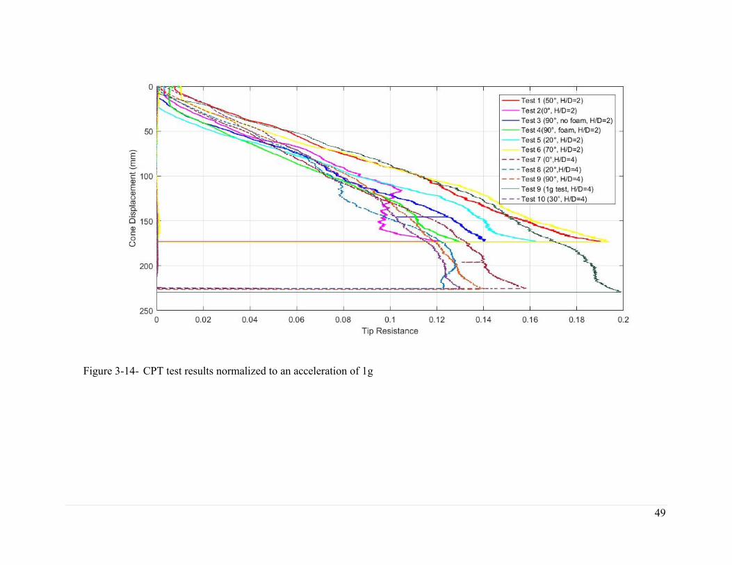
To allow for easier comparison of the CPT data sets, the data was scaled based using a factor

of 1 : N (Taylor, 1999). The results of the combined CPT tests are shown in Figure 3-14. The

shallow CPTs show more variation than the deep CPTs, which may be caused by soil density

variation through the initial sand raining process as they were the first tests completed. As the

test program continued, the variation in soil density between testbeds was reduced. The slopes of

the CPT data sets demonstrate that a similar density was attained for each test regardless of the

slight slope variations. The densities were also confirmed with standard density calculations

based on the weight and volume of the payload. The densities are listed in Table 3-2.

40

Table 3-1 - Centrifuge strongbox and pipe model parameters

Parameter Value

Shallow

Tests

Deep

Tests

Acceleration field, g 6.25 13.25

Pipe diameter (mm) 46

Centrifuge strong box (mm x mm x mm) 1180 x 940 x 400

Pipe length to diameter ratio, L/D (#) 8

Pipe burial depth at springline to diameter ratio, H/D (#) 2 4

Modeled pipeline diameter (mm) 304 609.5

Pipe length with sensors (mm) 533

Table 3-2 - Mobilization Angle and Density of Tests

Test ID Acceleration

Field

Burial Depth Angle of

Movement

Density (kg/m3)

1 6.25 2D 50° 1475

2 6.25 2D 0° 1453

3 6.25 2D 90° ( no

foam)

1460

4 6.25 2D 90°

(foam)

1468

5 6.25 2D 20° 1450

6 13.25 4D 70° 1475

7 13.25 4D 0° 1483

8 13.25 4D 20° 1465

9 13.25 4D 90° 1470

9 – Post 1 N/A N/A 1470

10 13.25 4/D 30° 1475

41

Figure 3-1 – Schematic diagram of shallow and deep pipe embedment depth

Figure 3-2- Pipe Set-up within Strongbox (Debnath, 2016)

42

Figure 3-3- Pipe assembly (1) including biaxial load cell (2, 3), stanchions (4, 5), dog bone

(6), and back bracket (7).

Figure 3-4- Major elements of the centrifuge test apparatus („payload‟) including dog bone

(6), ball race (7, 8), LVDT (9), guiding plate (10), motorized carriage (11), laser (12), and

cone (13).

43

Figure 3-5 – Pipe assembly (1) in strongbox after bedding layer including back bracket (7),

acoustic foam (14), and laser target (15).

Figure 3-6- Load cell configuration, based on Stroud (from Debnath, 2016)

Longitudinal webs Horizontal webs

44

Figure 3-7- Load cell dimensions and schematic used for lateral load (from Daiyan, 2011)

Figure 3-8- Load cell calibration apparatus used for lateral and axial loading

Axial loading

Lateral loading

45

Figure 3-9- Crushable Acoustic Foam after Test 8, 20°, H/D=4D

Figure 3-10- Sieve analysis results for sand used in testing

0%

10%

20%

30%

40%

50%

60%

70%

80%

90%

100%

0.01 0.1 1 10

% P

assi

ng

Sieve Size (mm)

Sample 1

Sample 2

Sample 3

46

Figure 3-11 Simplified direct shear testing apparatus

47

Figure 3-12- Cone penetration tests results for shallow burial depth tests (H/D=2)

48

Figure 3-13 - Cone penetration test results for deep burial depth tests (H/D=4)

49

Figure 3-14- CPT test results normalized to an acceleration of 1g

50

4. Experimental Results

4.1. Overview

A series of ten reduced scale centrifuge tests were completed at the C-CORE facility. The raw

data was collected and analyzed using MATLAB and Excel. This chapter will present the results

of these tests and compare the results to previous research.

A series of six tests were completed at a spring line burial depth of 2D and were considered

the shallow tests. As shown in Figure 4-1, the tests were completed at the following angles: 0°,

20°, 50°, 70°, 90°, and 90°. One of the 90° tests was completed without the acoustic foam to

allow for a comparison of the loading results. During the final shallow test at 70°, Test 6, the

sensor cables came loose during the test and caused faulty readings starting at a true mobilization

of approximately 15mm. The load cells were not damaged during Test 6 (H/D = 2; 70° attack

angle). The raw data from all of the shallow tests can be found in Appendix B.

A series of five tests were completed at a spring line burial depth of 4D and were considered

the deep tests. As shown in Figure 4-2, the tests were completed at the following angles: 0°, 20°,

30°, and 90°. During testing, the increased loads due to the deeper burial depth during all four

tests caused additional bending of the dog bone pieces and may have affected the results. After

the first deep test, a second dog bone was added to stiffen the setup and to help minimize the

bending. However, bending was still visually noted during testing, as shown in Figure 4-3.

During Test 9 (90°), the force of the stanchions pulling the model pipe was higher than the

resistance provided by the load cells and dog bone pushing inward to the pipe. The load cell

reading dropped to zero load at a displacement distance of approximately 2D, which indicated

51

that the pipe was pushed out from between the two stanchions. The pipe was pushed out with

enough force to cause the ball bearing to etch into the front of the load cell during test failure,

shown in Figure 4-4. During Test 10 (H/D = 4; 30° attack angle), the seal on the actuator failed

at a mobilization of approximately 2.1D, shown in Figure 4-5. No additional tests could be

conducted after the seal failed. The loads measured during the deep tests were approximately

25% higher than expected. Based on the equations proposed by ALA (2005), Honegger and

Nyman (2001), and PRCI (2004), the expected loads were approximately 1.5kN/m while the

highest loads measured were 2kN/m These higher than expected loads may have been caused by

several factors including the increased resistance and weight caused by the amount of

overburden sand, bending of the stanchions, and the rotation of the pipe assembly, which is

discussed below. The raw data from all four deep tests is included in Appendix B.

52

4.2. Pipe Mobilization

As discussed in Chapter 3, the mobilization distances were measured using two lasers. One

of the lasers was mounted on the actuator and the second was mounted on the dogbone. As

shown in Figure 4-6 and Figure 4-7, the laser mounted on actuator showed a larger overall

displacement than the laser mounted on the dogbone. The true displacement of the pipe cannot

be measured directly using the current the testing set up as the sand covers the pipe. The pipe is

unable to move as quickly as the motor since the sand creates additional resistance for the pipe to

overcome. The pipe lag, as shown in Figure 4-8, causes a larger measured mobilization at the top

of the stanchion as the pipe assembly rotates during testing. Daiyan (2013) recommended the

following displacement correction equation, which was used to correct the pipe displacements

for this research as it helps to correct for the pipe lag:

Eq. 4-1

( )

The difference in displacement between the two lasers varied from 7 to 9 mm (0.11D) during

the shallow tests. During the shallow tests, the pipe was mobilized a true corrected distance of 35

to 51mm or 0.7 to 1.1D for each respective test. During the unloading of the pipe assembly, the

difference in displacement noted between the two lasers was negligible.

During the deep tests, the difference in displacement varied from 11 to 18 mm, and the pipe

was mobilized 60 to 101.2mm. This corresponds to approximately 1.3 to 2.2D if Eq. 4-1 is used.

During each unloading cycle, the difference between the displacement measurements increased

from 0 mm to 5-8mm to 11-18 mm. This is due to the increased lag caused by the rotation of the

pipe assembly. This is similar to the ratcheting effect explained in Section 2.3. The increased lag

53

during the deep tests requires a refinement of equation 4-1 as the equation was determined using

the resistance caused by an H/D ratio of 2. It is expected that the equation would be closer to:

Eq. 4-2

( )

This equation would require an in-air test similar to the one conducted to determine the

original equation to confirm if it is accurate. This equation has been based deflection calculations

which found that the max deflection would be approximately 0.2D. The deflection calculations

assumed that the stanchion behaved like a cantilever beam fixed at the actuator.

To help confirm the finite element models based on this series of tests, which may be

completed by another researcher, the pipe assembly was loaded and then unloaded several times.

This cyclical loading will allow for better verification of the input soil properties by providing

information on the elastic behaviour of the soil (Daiyan, 2013). Information on the mobilization

distances is presented in Section 3.3.

54

4.3. Test Results and Analysis

During testing, the actual lateral and axial loads were measured using load cells placed on

either side of the pipe, and the displacements were measured using lasers. To facilitate the

comparison of data, all of the load results were normalized using the following equation:

Eq. 4-3

where the normalized load (Pt) was defined as the real force per unit length (Pu/L) divided by

the unit weight of the soil (γ), the spring line burial depth (H), and the pipe diameter (D). The

corrected mobilization distance was divided by the pipe diameter to provide a normalized

horizontal mobilization that could be easily compared to previous research (Kenny et al., 2015).

The results of the tests have been plotted as normalized load, y-axis, versus the corrected

displacement, x-axis. The primary information shown on the graphs are the peak load, and the

mobilization displacements to reach the peak load, also known as the ultimate yield

displacement. Based on previous research the ultimate yield displacement proposed by the ALA

(2005) is 0.1D for cohesionless soils and 0.2D for cohesive soils while previous reduced-scale

model experiments have shown an ultimate yield displacement is closer to 1D (Kenny and Jukes,

2015). It should be noted that the results from Test 6 (70°, H/D=2D) have not been included in

the analysis due to the failure of the cable leads. The normalized lateral load compared to the

corrected displacement for the shallow tests are shown in Figure 4-9, and the normalized axial

load as a function of the corrected displacement is shown in Figure 4-10.

55

Since loose sand was used during testing, a clearly defined peak load was not evident in the soil

load-pipe displacement data (see Figure 4-9 and Figure 4-10). The lack of clearly defined peak

load demonstrated a slight tangent hardening modulus with increasing displacement and that a

different method to define the peak load would have to be used. To define the peak load, three

methods have been proposed (Pike et al. 2011). The three methods are as follows and shown in

Figure 4-11:

1 – The peak load is defined as the point of intersection of the tangents to curve at small and

large displacements (Wantland et al. 1982).

2 – The peak load is defined as the point where load-displacement curve becomes a steep straight

tangent based on Terzaghi‟s definition of local failure.

3 – The peak load is defined as the true peak load at a large displacement.

For this research, the first and second methods have been used to define the peak load and the

corresponding mobilization distances, which were also used by both Daiyan et al. (2013) and

Debnath et al. (2015). The variation in peak load and mobilization between these two methods

can vary by up to 15% depending on the shape of the loading and displacement curve.

4.3.1. Pure Axial

Two axial tests, one at the shallow burial depth (Test 2, 0°, H/D=2) and one at the deep burial

depth (Test 7, 0°, H/D=4) were conducted as a part of this research. The normalized axial loads

and displacements for these tests are shown in Figure 4-12.

The normalized peak yield value for the shallow test (Test 2), using both Method 1 and 2 was

determined to be 4kN at a normalized yield displacement of 0.1D. As shown in Figure 4-13, the

56

shallow tests showed nearly twice the peak load noted in Debnath‟s centrifuge test which was

conducted at a higher acceleration (2015), and nearly four times the peak load noted in Hsu et al.

full model tests (2001). The peak load is 5% less than loads proposed by Schaminee et al. (1990).

This peak load may not be an accurate reading as the cyclical loading and unloading may have

affected the results. The normalized axial loads decreased to -2.5kN or 16 kPa, each time the

actuator was reversed. The slope of the unloading and loading as a function of displacement are

similar which indicates that the trailing and leading edge are flipped during the cyclical loading

and that the behaviour of the soil is consistent in both directions. These results are similar to the

cyclical loading responses noted during the previous reduces scale tests conducted by Nasser

(2013).

The mobilization distance of 0.1D associated with the peak axial load for the shallow test is

consistent with the mobilization distance as proposed by ALA (2005). The boundary conditions,

i.e. the foam selected for in front the stanchions, allowed for a displacement result closer to the

expected results.

For the deep test (Test 7) the peak yield value for the deep test is either 6.2kN with a

mobilization distance of 0.5D, using Method 1 to determine the peak load, or 7.9kN with a

mobilization distance of 0.6D if Method 2 is used. The load-displacement relationship shown in

Figure 4-12 increased much more gradually than that of the shallow axial test. During the two

unloading portions of the tests, the normalized loads decreased by 1kN and 2kN respectively.

This is one-third of the decrease noted during the shallow tests. The additional weight and

pressure of the soil above and in front of the pipe would have minimized the amount of uplift and

soil deformation around the foam and stanchion.

57

The peak loads shown in Figure 4-13, are approximately twice the peak loads noted during

the shallow tests conducted during this research using Method 2, or the research conducted by

Debnath in dense, shallow conditions (2015). These results are in line with the ALA guidelines

as the peak load increased at the same rate as the increased burial depth.

The mobilization distances of 0.5D and 0.6D are both approximately ten times higher than

what is expected by the ALA guidelines but are in line with the mobilization distances found

during dense sand testing (Daiyan, 2013, Debnath 2015, Hsu, 2010). The true mobilization

distances may be closer to the expected values since the mobilization corrections may not be

accurate because of the increased lag caused by the pipe assembly rotation during the deep tests

as discussed in Section 4.2. If the corrected mobilization distance equation proposed in 4.2 is

used, the corrected mobilization would be 0.33D and 0.42D respectively which is closer to the

ALA guidelines.

4.3.2. Pure Lateral

A total of three pure lateral tests were conducted as a part of this research. As shown in

Figure 4-14, one of the shallow tests was completed without foam, while the second shallow test

included foam on the leading side of both stanchions and both were mobilized to a distance of

0.9D. During the third test, which was conducted at a springline burial depth of 4D, the pipe

mobilization was stopped at 1.2D since bending was visually noted in the dog bones. A true peak

of 8 kN was noted in the results. Method 2 was used to determine the peak loads for the shallow

tests as no true peak was evident in the results. The peak loads are shown in Table 4-1.

Previous research including analytical models and physical modelling results have correlated

the normalized lateral loads to the spring line burial depth and soil properties (e.g. Audibert &

58

Nyman, 1977; Trautman & O‟Rourke, 1985; Smith, 1962; Debnath, 2016). The soil properties

used as variables include soil density and soil friction angle. For the lateral tests conducted as a

part of this research, the friction angle was 29°, and the average soil density used was

1467 kg/m3.

As shown in Figure 4-15, the results of Test 3, with foam, correspond well with the previous

research especially those of Debnath (2016) and Audibert and Nyman (1977) with a friction

angle of 35°. The result shown for Test 2, no foam, is similar to the results of Audibert and

Nyman for soil with an internal friction angle of 30° . The variation in these results may be

caused by the lack of foam in front of the stanchions during test 2. The foam increased the

measured peak load and mobilization by 27% for an identical acceleration and mobilization

sequence. These results are much closer to the estimated results. The test with foam (Test 3) also

showed more of elastic behaviour response of the soil when compared to the test without foam

(Test 2). This helps confirm the importance of the foam in front of the stanchions, which was

used to minimize their effects on the end boundary conditions.

The normalized loads from the deep tests are 1.5 times larger than the expected values for a

burial depth of 4D. It is assumed that this variation is caused by the stanchion dragging and the

additional rotation of the pipe assembly, which would have increased the observed loads. If the

stanchion is assumed to be similar to a cantilevered beam, the maximum deflection would be

approximately 0.2D. A stiffer pipe assembly may provide results closer to the results expected

based on ALA guidelines and help reduce the amount of pipe lag.

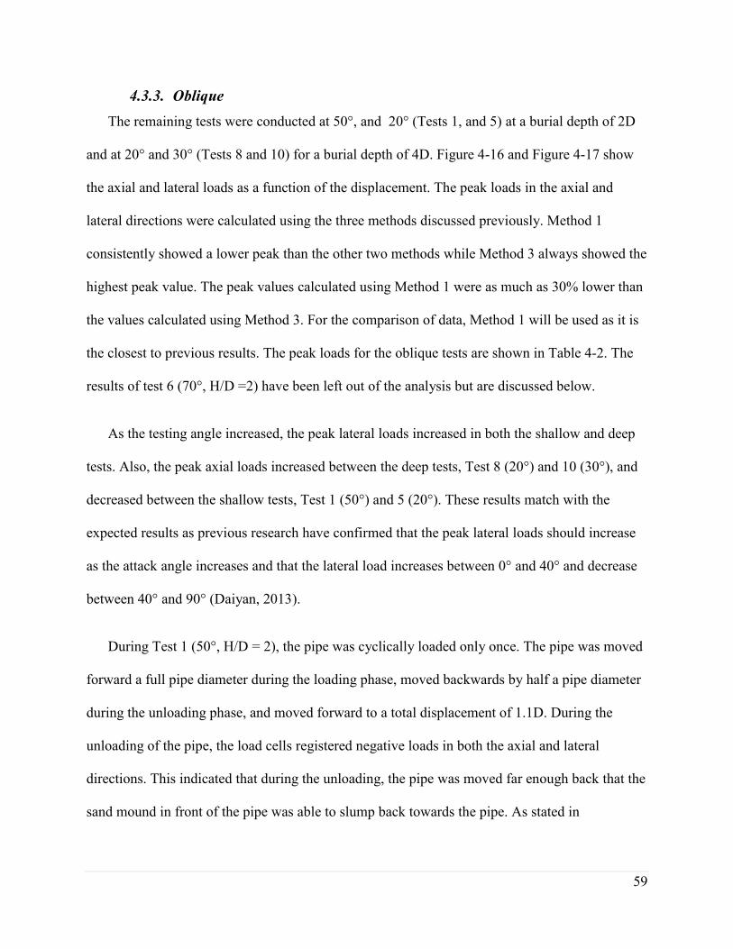
59

4.3.3. Oblique

The remaining tests were conducted at 50°, and 20° (Tests 1, and 5) at a burial depth of 2D

and at 20° and 30° (Tests 8 and 10) for a burial depth of 4D. Figure 4-16 and Figure 4-17 show

the axial and lateral loads as a function of the displacement. The peak loads in the axial and

lateral directions were calculated using the three methods discussed previously. Method 1

consistently showed a lower peak than the other two methods while Method 3 always showed the

highest peak value. The peak values calculated using Method 1 were as much as 30% lower than

the values calculated using Method 3. For the comparison of data, Method 1 will be used as it is

the closest to previous results. The peak loads for the oblique tests are shown in Table 4-2. The

results of test 6 (70°, H/D =2) have been left out of the analysis but are discussed below.

As the testing angle increased, the peak lateral loads increased in both the shallow and deep

tests. Also, the peak axial loads increased between the deep tests, Test 8 (20°) and 10 (30°), and

decreased between the shallow tests, Test 1 (50°) and 5 (20°). These results match with the

expected results as previous research have confirmed that the peak lateral loads should increase

as the attack angle increases and that the lateral load increases between 0° and 40° and decrease

between 40° and 90° (Daiyan, 2013).

During Test 1 (50°, H/D = 2), the pipe was cyclically loaded only once. The pipe was moved

forward a full pipe diameter during the loading phase, moved backwards by half a pipe diameter

during the unloading phase, and moved forward to a total displacement of 1.1D. During the

unloading of the pipe, the load cells registered negative loads in both the axial and lateral

directions. This indicated that during the unloading, the pipe was moved far enough back that the

sand mound in front of the pipe was able to slump back towards the pipe. As stated in

60

Section 4.2.1, the negative loads may have affected the peak axial loads, and in the future, the

pipe should not be unloaded as much to ensure the soil does not have the opportunity to slump.

Tests 5 (20°, H/D = 2), 8 (20°, H/D = 4), and 10 (30°, H/D = 4) were all loaded and unloaded

twice. The load-displacement graphs for all three graphs do not show a reversal of loading on the

load cell, which indicates that the loading-unloading cycles are correct. The shape of the shallow

test, Test 5(20°, H/D = 2), displays a more idealized load-displacement relationship for both the

axial and lateral tests. The graphs for Tests 8 (20°, H/D = 4), and 10 (30°, H/D = 4), also

resemble an idealized load-displacement relationship, but the graphs are much „noisier‟, i.e.

show more variation in the results. The increase resistance on the stanchions could have caused

this noise during loading and unloading caused by the deeper sand. The additional resistance and

rotation of the pipe assembly, shown by the lag, which has been previously discussed, and the

bending of the dog bone, may have also created oscillations through the stanchions as the pipe

was being dragged through the deeper sand. These oscillations show that a stiffer pipe assembly

is required for future deep burial depth tests as they have affected the test results.

The results of this research for shallow burial depth tests show higher loads than previous

full-scale models (Hsu et al., 2006) and lower loads than previous reduced scale (Kenny et al.,

2015) as shown in Figure 4-18. The oblique test results for Tests 1 (50°, H/D = 2), 5 (20°, H/D =

2), and 10 (30°, H/D = 4) all fall well within the proposed failure envelope previously proposed

by Daiyan (2013). A more refined failure envelope for this series of shallow tests, which

assumes that the failure mechanism changes from soil failure to pipe failure at an attack angle of

30° is shown as a green dashed line on the graph. The results for Test 5 (20°, H/D = 2), when

compared to other results, shows a much higher lateral load than expected while the axial load is

in line with previous research. In the post-test surface scan, as shown in Figure 4-19, the lateral

61

portion of the mounded sand is much larger than expected. This additional mounding may be

caused by soil ratcheting and caused an increase in the loads. Non-cyclical loading would have

reduced the ratcheting effect but would not have allowed for the confirmation of the elastic

behaviour of the soil.

The results of the deep tests (H/D=4) are also shown in Figure 4-13, but previous research

has not been completed at the same burial depth. As previously stated the loads are higher than

expected especially in Test 8 (20°), which falls outside of the expected soil mass failure envelope

and is shown as the dotted blue line on the graph. No oblique test was completed at an attack

angle larger than 30° but less than 90°.

During Test 6 at 70°, the load cell cables came completely detached during the test at a

mobilization of approximately 0.3D. Once the cables were detached the load reading varied

from 10000N to -10000N. Before the cables became detached, the normalized axial and lateral

loads did not follow the expected shape and are noisier than other shallow tests, as shown in

Figure 4-20 and Figure 4-21. This may be due to the fact the cables were loosened at some

unknown point during or before the test, and the results are not accurate. The load cells were not

damaged during this test, and the calibration matrices were re-confirmed after the test. The full

test results for this test are shown in Appendix B.

62

4.3.4. Uplift

As stated in Section 3.5, three LVDTs were used to measure the vertical movement of the

pipe assembly and settlement of the sand. During testing, as the pipe was pulled through the

sand, the leading end of the pipe and a soil column above the pipe were pushed up causing a

small sand mound in front of the pipe and a void space behind and above the pipe. Scans of the

sand surface were taken after each test to show the mounding and are shown in Appendix D. As

shown in the scans; the sand mounds were most noticeable in the shallow tests. The vertical

displacement of the pipe is also higher in shallow tests, which is what is expected based on the

sand mounds. Figure 4-22 shows the results from the two LVDTs mounted on the dog bones

from Test 4 (90°, H/D=2), which shows a typical shallow test result. The uplift measured for

each test was approximately 2 mm or 0.04D, which is 12mm when scaled to 1g. As shown in the

in the figure, during the unloading, the leading edge of the pipe does not fall back to its original

position which shows the ratcheting explained in Section 2.3.3. If the cyclical loading had not

been used, the vertical uplift would have been much lower and may have been much closer to the

finite element model predicted uplift (Daiyan, 2013, Kenny and Jukes, 2015).

The third LVDT was placed in the corner of the strong box to measure the settlement of the

sand during the acceleration of the payload. This LVDT was placed during Tests 3 (90°, H/D=2),

5 (20°, H/D=2), 6 (70°, H/D=2), 7 (0°, H/D=4), 8 (20°, H/D=), 9 (90°, H/D=4), and 10 (30°,

H/D=4). The results are shown in Figure 4-23. The readings from this LVDT show that the

settlements for the shallow tests vary from 0.38 to 0.75mm true displacement which is a

settlement of approximately 0.2 to 0.3% of the sands overall thickness. For the deep tests, where

the acceleration was 13.25G instead of 6.25G, the soil settled between 0.7 to 1.15mm or 0.2 to

63

0.35% of the sand thickness. Since the localized densification of the sand due to acceleration was

less than 0.5% and did not likely occur on the surficial layers, the sand is still considered loose.

By comparing the readings from the dogbone LVDTs and the soil LVDT, it was noted that

the pipe settled more than the surrounding sand during acceleration. This additional initial

settlement of the pipe assembly may have also skewed the results as the surrounding soil would

have been disturbed by the settlement. The pipe assembly was reduced in weight between

Daiyan (2013) and Debnath‟s (2015) research and could be further lightened to minimize the

effects of the pipe‟s self-weight during payload acceleration.

64

Table 4-1 – Peak lateral load results and corresponding mobilization

Test ID Peak Load Normalized

Displacement

2 – no foam 8 0.2D

3 – foam 11 0.3D

9 20 0.9D

Table 4-2 - Peak axial and lateral loads - oblique tests

Test ID Method 1 Method 2 Method 3

# Angle (°)

Peak

Lateral

Load

(kN)

Peak

Axial

Load

(kN)

Peak

Lateral

Load

(kN)

Peak

Axial

Load

(kN)

Peak

Lateral

Load

(kN)

Peak

Axial

Load

(kN)

1 50 7.3 3.2 8.7 3.8 9.2 4.4

5 20 11 3.8 12.3 5 17 6.8

8 20 7.8 6 9 7 9.8 8.2

10 30 12.4 6.2 13.6 6.8 14.2 8

65

Figure 4-1 – Pipe orientation of shallow tests (Test 1 – 6, H/D=2)

Figure 4-2 – Pipe orientation of deep tests (Tests 7-10, H/D=4)

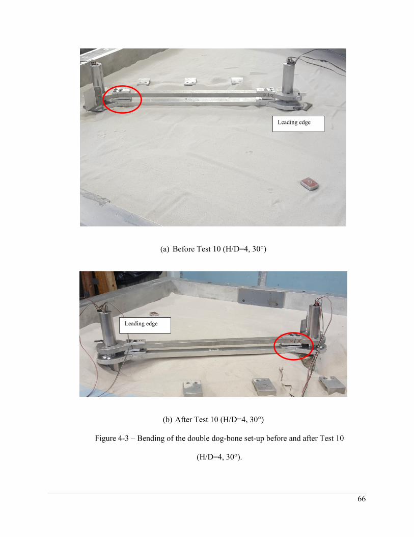
66

(a) Before Test 10 (H/D=4, 30°)

(b) After Test 10 (H/D=4, 30°)

Figure 4-3 – Bending of the double dog-bone set-up before and after Test 10

(H/D=4, 30°).

Leading edge

Leading edge

67

Figure 4-4 - Load cell A after model pipe was pulled out from between stanchions

(Test 9, 90°, H/D=4)

Figure 4-5 - Motor seal failure after final test (Test 10, 30°, H/D=4)

Damage cause by ball earing is

circled in red

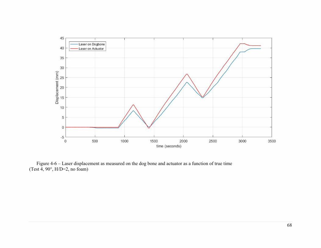
68

Figure 4-6 – Laser displacement as measured on the dog bone and actuator as a function of true time

(Test 4, 90°, H/D=2, no foam)

69

Figure 4-7 - Laser displacement as measured on the dog bone and actuator as a function of true time (Test 10, 30°, H/D=4)

70

Figure 4-8 – Schematic of idealized pipeline lag during mobilization

71

Figure 4-9 – Lateral Loads (normalized) as a function of corrected pipe movement (shallow tests)

72

Figure 4-10 - Normalize axial loads as a function of corrected pipe movement (deep tests)

73

Figure 4-11 - Schematic illustration of peak load determination

(Pike et al. 2011, from Debnath, 2016)

74

Figure 4-12 – Results of pure axial tests as a function of pipe diameter (Test 2- H/D=2, Test 7- H/D=4)

75

Figure 4-13 - Comparison of axial test results to existing data

(variation to Kenny et al., 2015)

0

1

2

3

4

5

6

7

8

0 0.2 0.4 0.6 0.8 1

No

rmal

ize

d A

xial

Yie

ld F

orc

e

Normalized Axial Yield Displacement

Schaminee et al. (1990)

ALA (2005)

Daiyan (2013) - Dense; H/D= 2

Debnath (2015) - Dense;H/D = 2

Debnath (2015) - Loose; H/D= 2

Hsu et al. (2001) - Loose;H/D = 1

Hsu et al. (2001) - Dense;H/D = 1

Marcotte (2017) - Loose;H/D = 2

Marcotte (2017) - Loose;H/D = 4 - Method 1

Marcotte (2017) - Loose;H/D = 4 - Method 2

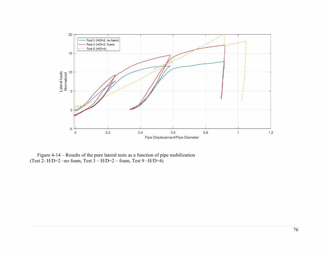
76

Figure 4-14 – Results of the pure lateral tests as a function of pipe mobilization

(Test 2- H/D=2 –no foam, Test 3 – H/D=2 – foam, Test 9 –H/D=4)

77

Figure 4-15 - Comparison of lateral test results in loose sands (variation on Kenny et al., 2015)

0

5

10

15

20

25

0 2 4 6 8 10 12 14

Nh

H/D

Current Research, D=609mm

Current Research, D=304mm

Debnath(2016), ϕ=36°, D=609mm, ρ=14.6kN/m3

Guo& Stoll (2005), D=609mm,n=0.2, k=3, m=0.35

Trautmann & O'Rourk (1985) Oversen (1964), ϕ=35°

Audibert & Nyman (1977), Hansen (1961), ϕ=30°

Audibert & Nyman (1977), Hansen (1961), ϕ=35°

78

Figure 4-16 - Normalized axial load as a function of pipe displacement for oblique tests

(50° -H/D=2, 70° -H/D =2, 20° - H/D=4, 30° - H/D=4)

79

Figure 4-17 – Normalized lateral load as a function of the true pipe displacement for oblique tests

(50° -H/D=2, 70° -H/D =2, 20° - H/D=4, 30° - H/D=4)

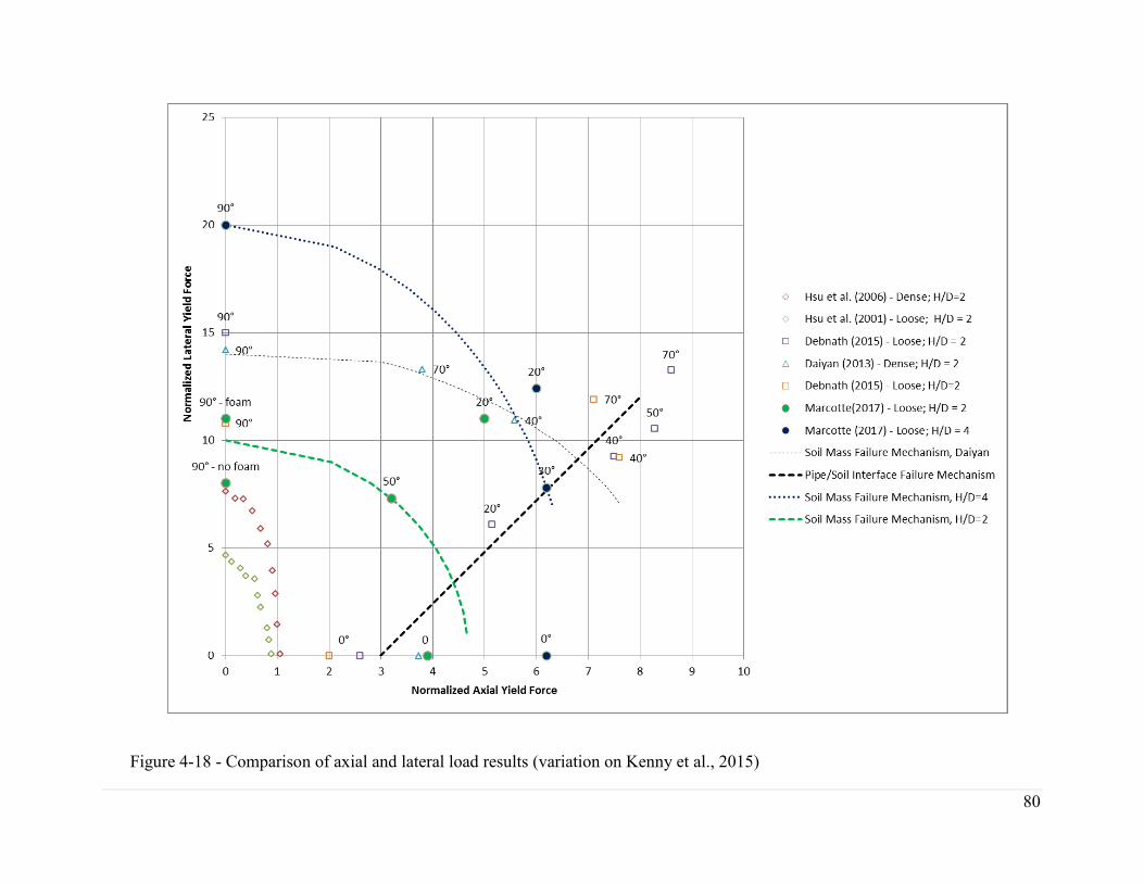
80

Figure 4-18 - Comparison of axial and lateral load results (variation on Kenny et al., 2015)

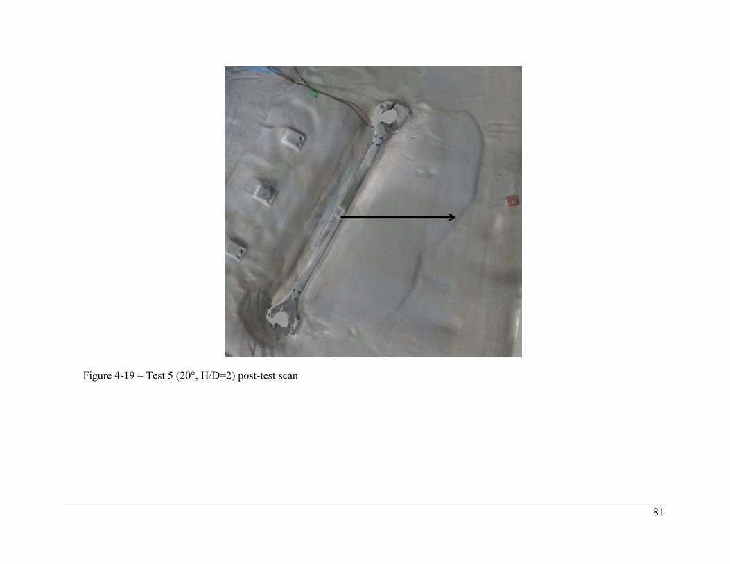
81

Figure 4-19 – Test 5 (20°, H/D=2) post-test scan

82

Figure 4-20 - Normalized lateral load as a function of pipe displacement

(Test 6, 70°, H/D=2)

Figure 4-21 - Normalized axial loads as a function of pipe displacement

(Test 6, 70°, H/D=2)

83

Figure 4-22 – Uplift displacement of leading and trailing edge of dogbone (Test 4, 90°, H/D=2)

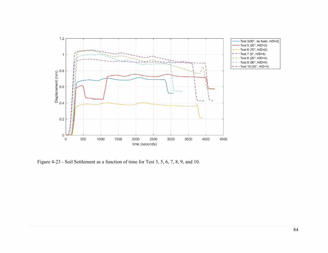
84

Figure 4-23 - Soil Settlement as a function of time for Test 3, 5, 6, 7, 8, 9, and 10.

85

5. Summary and Conclusions

A series of ten reduced-scale tests were completed at different attack angles in loose silica

sand with a friction angle of 29°. All ten tests were conducted using a similar testing procedure

with respect to the test bed preparation, instrumentation type, number and placement, and

treatment of boundary conditions using the acoustic foam. The pipe was cyclically loaded during

testing to confirm the elastic behaviour of the soil and consistency of the test bed condiotion. The

purpose of the research was to measure the soil yield load and yield displacement response and

determine the failure envelope.

Six tests were completed at an H/D ratio of 2 and were considered the shallow tests. The tests

were completed at the following angles: 0°, 20°, 50°, 70°, and two tests at 90°. One of the 90°

tests was completed without the acoustic foam in front of the stanchions to determine the effects

of the foam during testing. The ultimate lateral and axial loads determined during testing were

similar to the results from the previous centrifuge and finite element research (Daiyan, 2013,

Debnath, 2015), which were greater than measurements obtained during full-scale physical

modelling (Hsu, 2010). In comparison with previous research, the mobilization distances at yield

loads from this research were much closer to the mobilization distances proposed by the ALA

guidelines (2005). This was particularly evident when comparing the mobilization distances

developed for the 90° test using the acoustic foam, which was consistent with the ALA

guidelines, with the same test without using the foam inserts.

A series of five tests were also completed at a spring line burial depth of 4D, which were

considered the deep tests. These tests were completed at the following angles: 0°, 20°, 30°, and

90°. During testing, the increased loads due to the deeper burial depth during all five tests caused

86

additional bending of the dog bone pieces and a rotation of the pipe assembly. The measured

yield loads and mobilization distances were greater than the ALA guideline predictions (2005).

The discrepancy was attributed to mechanisms developed in the test frame during the test

including pipe lag and pipe assembly rotation, which may have reached up to 0.2D deflection

magnitude. The lag was caused by insufficient stiffness of the test frame and was affected by the

increased resistance of the additional weight of the soil above the pipe. This mechanism resulted

in the failure of the test assembly and load cell. Before further deep tests can be conducted, the

pipe assembly would require improvements to ensure that additional errors are not introduced to

the results by the rotation of the pipe assembly.

5.1. Future Research and Recommendations

This research is part of a larger body of studies on pipe/soil interaction and provides

complementary evidence supporting and extending the database on oblique pipe/soil interaction

events. To help improve the knowledge base, it is recommended that additional research be

conducted to further confirm the assumptions and results from this research.

5.1.1. Future Reduced Scale Test

Before additional reduce scaled tests are conducted, the following improvements to the

reduced scale testing methodology are proposed:

- Reinforcement of the pipe assembly and frame, especially for the deep tests. This

reinforcement would help minimize the rotation of the stanchions during mobilization

and minimize the error caused by the pipe movement lag during testing. A possible

option is to include a tensioned rod connecting the two load cells to ensure that the model

pipe is not pulled from between the stanchions. Before this option could be used, the

87

effect of the rod on the end bearing conditions would need to be modelled as the load cell

would no longer be held in place with a pinned connection.

- Reduction of the weight of the pipe assembly by using a lighter composite material

especially if the assembly is reinforced to ensure that the weight is consistent with a real

pipe during testing.

- Introduction of additional instrumentation along the pipe and pipe assembly itself to

provide additional information during testing. Strain gauges could be added along the

pipe length and the stanchions, which would help quantify the bending that is occurring

during testing. A load cell may also be added to the top of the stanchions to measure the

loads on the stanchions during testing.

- Refinement of the loading/ mobilization pattern. A smaller amplitude of motion during

loading and unloading would minimize the effect of ratcheting and may provide more

accurate results for uplift modelling.

- Confirmation of the expected loads using numerical modeling before the reduce scale

tests are completed. This would help minimize the possibility of bending of the pipe

assembly during testing and failure of the motor due to the applied moments. For this

research, the expectant loads were calculated based on the ALA guidelines (2005) and a

safety factor of 1.5 was applied to ensure that the motor would have the capacity to

mobilize the pipe.

Future reduce scaled tests should also be conducted with different variables including burial

depths, saturation levels, and soil properties. Other possible tests may include additional tests

88

with an H/D of 4 but different densities and/or internal friction angle of sand and tests in

cohesive soils.

5.1.2. Soil Property and Characteristics

As additional tests are conducted with different types of cohesionless soils, the soil

characterization process should be refined for the reduced scale tests. Sieve analysis should be

conducted before and after the testing to confirm and quantify the changes to the gradation of the

soil caused by the testing procedure.

Triaxial tests, as opposed to simple shear tests, are recommended to determine the internal

friction of the soil. For this research, the shear tests were used due to the availability of the

equipment at the time of testing.

5.1.3. Verification Testing

Full-scale tests should be conducted with the same testing parameters as this research to

provide a comparison to this data set. The results of the full-scale tests conducted by Hsu (2010)

do not match the results of the reduced scale tests with similar parameters from Daiyan (2013) or

the practice guidelines. Since the previous reduced-scale tests, the methodology has been refined

and has shown results closer to the expected results.

5.1.4. Finite Element Modeling

A model using similar parameters as this research should be conducted to confirm if the

results are consistent with the finite element model proposed by Daiyan (2013). The previous

research by Daiyan was conducted at shallow depth using dense sands so these new testing

parameters can be used to validate his model.

89

It is also recommended that the effect of the stanchions be modelled to help estimate the

amount of rotation and bending of the stanchions during testing. It may also help quantify the

pipe lag which occurred during the deep tests. During modelling, different resistances could be

modelled in front of the stanchions to help determine which material would be the most effective

at minimizing the effect of the stanchions on the end bearing conditions.

5.1.5. Integration of Results

Once a sufficient amount of data is available including results from reduce-scaled tests, full-

scale tests, and numerical models, the results should be compared to help improve the existing

ALA guidelines and best-practice procedures. These improvements would include a more

accurate way to estimate the ultimate yield loads and displacements and will allow for a more

accurate model of multi-directional loaded pipelines. Updated failure envelopes should also be

developed based on the soil type and pipeline dimensions to allow for user-friendly design tables

or graphs for use in industry.

90

6. Bibliography

Abdoun, Tarek (2011). Centrifuge physical modeling & scaling laws. RPI/UCD NEES

Centrifuge Research and Training Workshop 2011.

American Lifeline Alliance (2001). Guidelines for the design of buried steel pipe, American

Lifeline Alliance (ALA), Federal Emergency Management Agency (FEMA),

Washington, D.C.

ALA 2005. Guidelines for the design of buried steel pipes. American Lifelines Alliance, 76p.

ASCE (1984). Guidelines for the seismic design of oil and gas pipeline systems. American

Society of Civil Engineers, Committee on gas and liquid fuel lifelines, Technical Council

on Life line Earthquake Engineering, ASCE, NewYork.

ASTM D3080 / D3080M-11, Standard Test Method for Direct Shear Test of Soils Under

Consolidated Drained Conditions, ASTM International, West Conshohocken, PA, 2011

Audibert, J. M. E. and Nyman, K. J. (1977). Soil restraint against horizontal motion of pipes.

Journal of Geotechnical Engineering Division, ASCE, 103(10), 111 9-11 42.

Balachowski, L. 2007. Size Effect in Centrifuge Cone Penetration Tests. Hydro-Engineering and

Environmental Mechanics. Vol 54 No. 3 pp. 191-181

Bolton, M. D., Gui, M.W., Garnier, J., Corte, J.F., Bagge, G., Laue,J., and Renzi, R. 1999.

Centrifuge Cone Penetration Tests in Sand. Geotechnique 49, No. 4 : 543 - 552

Burnett, A. 2015. Investigation of full scale horizontal pipe/soil interaction and large strain

behaviour of sand. M.A.Sc. Thesis, Queen‟s University, 118p.

91

Craig, W.H. 1995. Geotechnical centrifuge: Past, present and future. Geotechnical Centrifuge

Technology, pp.1-18.

Cheuk, C. Y., White, D. J ., Bolton, M. D. (2008). Uplift mechanisms of pipes buried in sand.

Journal of Geotechnical and Geoenvironmental Engineering, ASCE, 134(2).

Cocchetti, G., Prisco, C., Galli, A. and Nova, R. (2009a). Soil-pipeline interaction along unstable

slopes: a coupled three-dimensional approach. Part I : Theoretical formulation. Canadian

Geotechnical Journal, 46 (11 ): 1289-1304.

Cocchetti, G., Prisco, C., and Galli, A. (2009b). Soil-pipeline interaction along unstable slopes: a

coupled three-dimensional approach. Part 2: Numerical analysis. Canadian Geotechnical

Journal, 46 (11): 1305-1321. Canadian Geotechnical Society. 2006.

Daiyan, N. 2013. Investigating Soil/Pipeline Interaction During Oblique Relative Movements.

PhD Thesis, Memorial University of Newfoundland, 204p.

Daiyan, N., Kenny, S., Phillips, R. and Popescu, R. 2011. Investigating pipe/soil interaction

under axial/lateral relative movements in sand. Can. Geotech. J., 48(11): 1683-1695.

Daiyan, N., Kenny, S., Phillips, R. and Popescu, R. 2010. Numerical investigation of oblique

pipe/soil interaction in sand. Proc., IPC2010-31644:6p

Debnath, P. 2015. Centrifuge modeling of oblique pipe/soil interaction in dense and loose sand.

M.Eng. (Thesis), Memorial University of Newfoundland, 120p.

El Hmadi, K., O‟Rourke, J. 1988. Soil Spring for Buried Pipeline Axial Motion. J. Geotech.

Enrg. 114(11) 1335-1339

92

Garnier, J., Gaudin, C., Springman, S.M., et al. 2007. Catalogue of scaling laws and similitude

questions in geotechnical centrifuge modelling. Int. J. Phy. Mod. Geo., 7(3):1-23.

Gaudin, C., Randolph, M. and White, D. 2016. Centrifuge Modelling in Geotechnics. CRC

Press, ISBN 9780415522243, 544p.

Guo, P. (2005). Numerical modeling of pipe-soil interaction under oblique loading. Journal of

Geotechnical and Geoenvironmental Engineering, ASCE, 131 (2), pp. 260-268.

Guo. P. and Stolle. D. F. (2005). Lateral pipe-soil interaction in sand with reference to scale

effect. Journal of Geotechnical and Geoenvironmental Engineering, ASCE, 131 (3): 338-

349.

Hansen, J.B. (196 1). The ultimate resistance of rigid piles against transversal forces. Bulletin 12,

Danish geotechnical institute, Copenhagen, Denmark, pp.S-9.

Hodder, M. S. and Cassidy, M. J. (20 I 0). A plasticity model for predicting the vertical and

lateral behavior of pipelines in clay soils. Geotechnique, 60, o. 4, pp. 247-263.

Horvath, J. S. Colasanti. R.J 2011. New Hybrid Subgrade Model for Soil-Structure Interaction

Analysis: Foundation and Geosynthetics Applications. GeoFrontiers2011, ASCE.

Horvath, J. S. (2002). Soil-structure interaction research project; basic SSI concepts and

applications overview. Report No. CGT-2002-2, Manhattan Coil., Bronx, NY.

Honegger, D. G. (1999). Field measurements of axial soil friction forces on buried pipelines.

Proceedings of the Fifth U.S. Conference on Lifeline Earthquake Engineering, Technical

93

Council on Lifeline Earthquake Engineering, Monograph No. 16, American Society of

Civil Engineers.

Honegger. D. G., Hart, J. D., Phillips, R., Popelar. C. and Gailning, R. W. (201 0). Recent PRCI

guidelines for pipelines exposed to landslide and ground subsidence hazards. Proceedings

of IPC201 0, International Pipeline Conference, Calgary.

Honegger, D. G. and Nyman, J. (2004). Guidelines for the seismic design and assessment of

natural gas and liquid hydrocarbon pipelines. Pipeline Research Council International,

Inc., No.L5 1927.

Hsu, T.W., Chen, Y.J. and Hung, W.C.2006. Soil restraint to oblique movement of buried pipes

in dense sand." J. Transp. Eng. 132(2):175-181.

Hsu, T.W., Chen, Y.J. and Hung, W.C. 2001. Soil friction restraint of oblique pipelines in loose

sand. J. Transp. Eng. 127(1):82-87.

Jacky, J. (1944). The coefficient of earth pressure at rest. Journal of the society of Hungrian

Architects and Engineers, Budapest, Hungry, pp. 355-358.

Jardine, R. J., and Overy, R. F. (1996). Axial capacity of offshore piles driven in dense sand.

Proceedings Offshore International Conference, Houston, Texas, USA., pp. 161-180.

Karimian, S. A. (2006). Response of buried steel pipelines subjected to longitudinal and

transverse ground movement. PhD Thesis, The University of British Colombia.

94

Kennedy, R. P. , Chow, A. W., and Williamson, R. A. ( 1977). Fault movement effects on buried

oil pipelines, Journal of the Transportation Engineering Division, ASCE, vol. 103, pp. 6

17-633.

Kenny, S., Jukes, P. 2015. Pipeline/Soil Interaction Modeling in Support of Pipeline Engineering

Design and Integrity. John Wiley and Sons

Kenny, S. Pike, K., Debnath, P., and Hawlader, B. 2015. Integrated Framework in Support of

Pipeline Engineering Design for Geohazards. Geo Quebec 2015

Knut. S. 2016. Characteristic soil strength for axial pile capacity and its estimation with

confidence for offshore applications. Structural Safety Vol 63 pg. 81-89

Lam, S.Y., Ng. C.W.W., Leung C.F, Chan, S.H. 2009. Centrifuge and Numerical Modeling of

Axial Load Effects on Piles in Consolidating Ground. Canadian Geotechnical Journal

46.1

Liu, Q.B, Lehane, B.M. 2012. The influence of particle shape on the (centrifuge) cone

penetration test (CPT) end resistance in uniformly graded granular soils. Géotechnique:

Vol.62 Issue 11, pp. 973-984

Mackenzie, T. R. (1955). Strength of deadman anchors in clay. MSc. Thesis, Princeton

University , USA.

Maddock, D.V. 1981. The Development of a Transducer to Measure the Effective Soil Stresses

and the Pore Water Pressure Acting on the Surface of a Driven Steel Pile. Cambridge

University

95

Merifield, R. S. and Sloan, S. W. (2006). The ultimate pullout capacity of anchors in frictional

soils. Canadian Geotechnical Journal, 43, pp. 852-868.

Merifield, R. S., Sloan, S. W. and Yu, H. S. (2001). Stability of plate anchors in undrained clay.

Geotechnique 51, No.2, pp. 14 1-153.

Meyerhof, G. G. (1955). Influence of roughness of base and groundwater conditions on the

ultimate bearing capacity of foundations. Geotechnique, Vol. 5, pp. 227-242.

National Research Canada. 2016. 10 Key Facts on Canada‟s National Resources. NRC

Ng, P. C. F. (1994). Behavior of buried pipelines subjected to external loading. PhD Thesis,

University of Sheffield, England.

Ng, C. W. W., and Springman, S. M. (1994). Uplift resistance of buried pipelines in granular

materials. Centrifuge 94, Leung, Lee and Tan, eds., pp. 753-758.

Ng, C.W.W. (2014) The state of the art centrifuge modeling of geotechnical problems at

HKUST. Journal of Zhejiange University. Vol 15 Issue 1. Pp1-21.

Nobahar, A., Kenny, S. and Phillips, R. (2007). Buried pipelines subject to sub gouge

deformations. International Journal of Geomechanics, 7(3).

Nobahar, A., Popescu, R., and Konuk, l. (2000). Estimating progressive mobilization of soil

strength. Proceedings 53rct Canadian Geotechnical Conference, Montreal, Que., 15-18

Oct. 2000. Edited by D. Leboeuf Bi Tech Publishers Ltd., Richmond, B.C.

Nyman, K.J. (1984). Soil response against oblique motion of pipes. Journal of Transportation

Engineering, 11 0(2), pp. 190-202.

96

O'Rourke, T.D. (1989). Seismic design considerations for buried pipelines. Annals of the New

York academy of sciences, ISSN 0077-8923, Vol. 558, pp. 324-346.

O' Rourke, T.D., Turner, J.E., Jeon, S-S., Stewart, H.E, Wang, Y. and Shi, P. (2005). Soil-

structure interaction under extreme loading conditions, The 13th Spencer J. Buchanan

Lecture.

Ovesen, N. K. (1964). Anchor slab calculation methods and model tests. Danish Geotechnical

Institute, Copenhagen, Denmark, Bulletin 16, 40p.

Paulin, M. J., Phillips, R., Clark, J. I., Trigg, A., & Konuk, I. 1998. Full-scale investigation into

pipeline/soil interaction. Proc., CGS:241-248.

Phillips, R., Nobahar, A., and Zhou, J.2004a. Combined axial and lateral pipe-soil interaction

relationships. Proc., IPC-0144:5p.

Phillips, R., Nobahar, A., and Zhou, J.2004b. trench effects on pipe-soil interaction. Proc., IPC-

0141:7p.

Pike, K., Kenny, S., (2011) Advancement of CEL procedures to analyze large deformation pipeline

/soil interaction events, Proceedings of Offshore Technology Conference, Houston, Texas,

USA, May 2011.

Pike, K.P. and Kenny, S.P. 2012a. Lateral-axial pipe/soil interaction events: Numerical modeling

trends and technical issues. Proc., IPC-90055:6p.

Rossiter, C. and Kenny, S. 2012. Evaluation of lateral-vertical pipe/soil interaction in clay. Proc.,

OTC-23735:13p.

97

Rowe, R. K. (1978). Soil structure interaction analysis and its application to the prediction of

anchor behaviour. PhD thesis, University of Sydney, Sydney, Australia.

Rowe, R. K., and Davis, E. H. (1982a). The behaviour of anchor plates in clay. Geotechnique,

32(1 ), pp. 9-23.

Rowe, R. K., and Davis, E. H. (1982b). The behavior of anchor plates in sand. Geotechnique,

32(1 ), pp. 25-4 1.

Schaminee, P. E. L., Zorn, N. F., &Schotman, G. J. M. 1990. Soil response for pipeline upheaval

buckling analyses: Full-scale laboratory tests and modeling. Proc., OTC-6486:563-572.

Sherif. M. A., Fang, Y. S. and Sherif, R. I. (1984). K" and K0 behind rotating and on yielding

walls. ASCE Journal of Geotechnical Engineering, 110, pp. 41-56.

Stroud, M. A. (1971). Sand under low stress levels in simple shear apparatus. PhD thesis,

Cambridge University, Cambridge, UK.

Taylor, R. N. (1995). Geotechnical centrifuge technology. Blackie academic & professional,

London, 296p.

Trautmarm, C. H. (1983). Behavior of pipe in dry sand under lateral and uplift loading. PhD

thesis, Cornell University, Ithaca, New York.

Trautmann, C. H. and O' Rourke, T. D. (1985). Lateral force-displacement response of buried

pipe. Journal of Geotechnical Engineering, ASCE, 111 (9), pp. 1077-1 092.

Wantland. G. P., O'Neil, M. B., Coelogyne, E. H. and Reese, L. C. (1982). Pipeline lateral

stability in soft clay. Journal of Petroleum Technology, 34(1), pp. 217-220.

98

Wijewickreme, D., Karimian, A., Honegger, D.G. (2005). Effectiveness of some methods of

reducing axial soil loads on buried pipelines subjected to ground movements.

Proceedings of the 58th Canadian Geotechnical Conference, Saskatoon

Wijewickreme, D., Karimian, H. and Honegger, D. (2009). Response of buried steel pipelines

subjected to relative axial soil movement. Canadian Geotechnical Journal, 46, pp. 735-

752.

Winkler, E. (1867). Die Lehre Von Elastizitat und Festigkeit (Teachings on Elasticity and

Stiffness). Prague, Czechoslovakia, 182p.

Zhang, Y. (2004). Characterization of the Compressive and Fracture Behaviors, as well as the

Residual Tensile Strength of a Polyurethane Foam. Master of Science Thesis, Oklahoma

State University

Appendix A – Soil Properties

100

Figure A- 1- Shear Test Results of Silica Sand used in testing

101

Figure A- 2 – Normal stress as a function of shear stress

Table A- 1 - Sieve test results for silica sand used in testing

Test 1 Test 2 Test 3

Sieve Size (mm) Weight(g) %Passing Weight(g) %Passing Weight(g) %Passing

Initial Weight 1497.4 1946.8 985.7

2.36 0.2 100% 0 100% 0 100%

1 0.2 100% 0 100% 0 100%

1.18 0.2 100% 0 100% 0 100%

0.25 434.2 71% 998.2 49% 298.7 70%

0.15 1070.4 29% 1644.1 16% 684.5 31%

0.075 1464.6 2% 1934.7 1% 964.2 2%

0 1493.3 0% 1946.6 0% 985.2 0%

Difference -4.1 -0.2 -0.5

y = 0.4872x + 7.4293

0.000

10.000

20.000

30.000

40.000

50.000

60.000

70.000

80.000

0 20 40 60 80 100 120 140

She

ar S

tre

ss (

kPa)

Normal Stress (kPa)

Appendix B - Instrument Calibration

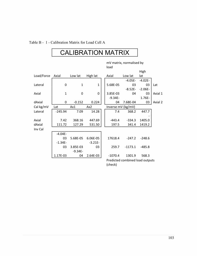
103

Table B - 1 - Calibration Matrix for Load Cell A

CALIBRATION MATRIX

mV matrix, normalised by load

Load/Force Axial Low lat High lat

Axial Low lat

High lat

Lateral 0 1 1

5.68E-05 -4.05E-

03 -4.02E-

03 Lat

Axial 1 0 0

3.85E-03 -8.52E-

04 -2.06E-

03 Axial 1

dAxial 0 -0.152 0.224

-9.34E-04 7.68E-04

1.76E-03 Axial 2

Cal kg/mV Lat Ax1 Ax2

Inverse mV (kg/mV) Lateral -245.94 7.09 14.28

7.4 368.2 447.7

Axial 7.42 368.16 447.69

-443.4 -334.3

-1405.0

dAxial 111.72 127.29 531.50

197.5 341.4 1419.2 Inv Cal

-4.04E-03 5.68E-05 6.06E-05

17618.4 -247.2 -248.6

-1.34E-03 3.85E-03

-3.21E-03

259.7 -1173.1 -485.8

1.17E-03

-9.34E-04 2.64E-03

-1070.4 1301.9 568.3

Predicted combined load outputs (check)

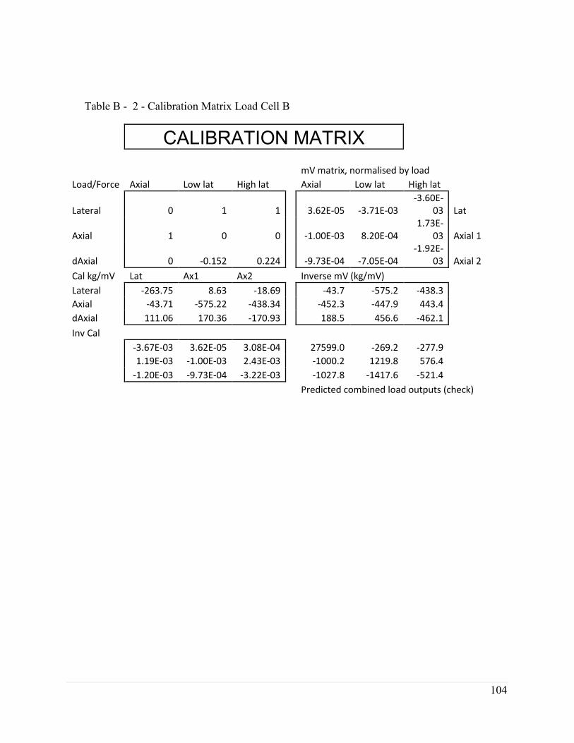
104

Table B - 2 - Calibration Matrix Load Cell B

CALIBRATION MATRIX

mV matrix, normalised by load

Load/Force Axial Low lat High lat

Axial Low lat High lat

Lateral 0 1 1

3.62E-05 -3.71E-03 -3.60E-

03 Lat

Axial 1 0 0

-1.00E-03 8.20E-04 1.73E-

03 Axial 1

dAxial 0 -0.152 0.224

-9.73E-04 -7.05E-04 -1.92E-

03 Axial 2

Cal kg/mV Lat Ax1 Ax2

Inverse mV (kg/mV) Lateral -263.75 8.63 -18.69

-43.7 -575.2 -438.3

Axial -43.71 -575.22 -438.34

-452.3 -447.9 443.4 dAxial 111.06 170.36 -170.93

188.5 456.6 -462.1

Inv Cal

-3.67E-03 3.62E-05 3.08E-04

27599.0 -269.2 -277.9

1.19E-03 -1.00E-03 2.43E-03

-1000.2 1219.8 576.4

-1.20E-03 -9.73E-04 -3.22E-03

-1027.8 -1417.6 -521.4

Predicted combined load outputs (check)

105

Figure B- 1 - LVDT 3031 Calibration

Figure B- 2 - LVDT 5080 Calibration

y = 0.2647x + 2.0864 R² = 0.9959

0

1

2

3

4

5

6

7

0 2 4 6 8 10 12 14 16

LVD

T R

ead

ing

(mV

)

Displacement (mm)

LVDT 3031

y = 0.2808x + 1.0212 R² = 1

0

1

2

3

4

5

6

0 2 4 6 8 10 12 14 16

LVD

T R

ead

ing

9m

V)

Displacement (mm)

LVDT 5080

Appendix C – Raw Test Data

107

Figure C- 1 – Unprocessed lateral load (N) as a function of true pipe displacement (mm) for

all ten reduced scaled tests.

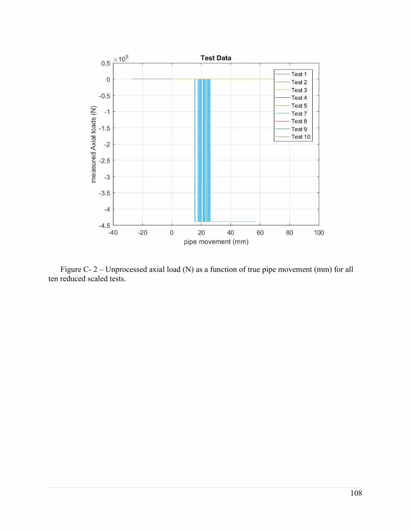
108

Figure C- 2 – Unprocessed axial load (N) as a function of true pipe movement (mm) for all

ten reduced scaled tests.

Appendix D – Test Scans

110

Figure D- 3– Post-test scan Test 1 (50°, H/D=2D, 6.5g).

Arrow shows direction of movement

111

Figure D- 4 – Post-test scan Test 2 (0°, H/D=2, 6.5g)

The arrow shows the direction of movement, and the dashed line shows pipe alignment.

112

Figure D- 5 – Post-test scan of test 3 (90°, H/D=2, no foam, 6.5g) without dog bone and with

dog bone

The arrow shows the direction of movement and the dashed line shows pipe alignment.

113

Figure D- 6 – Post-test scan of Test 4 (90°, H/D=2, with foam, 6.5g)

The arrow shows the direction of motion. The dashed line shows pipe alignment.

114

Figure D- 7 – Post-test scan of Test 5 (20°, H/D=2, 6.5g)

The arrow shows direction of movement

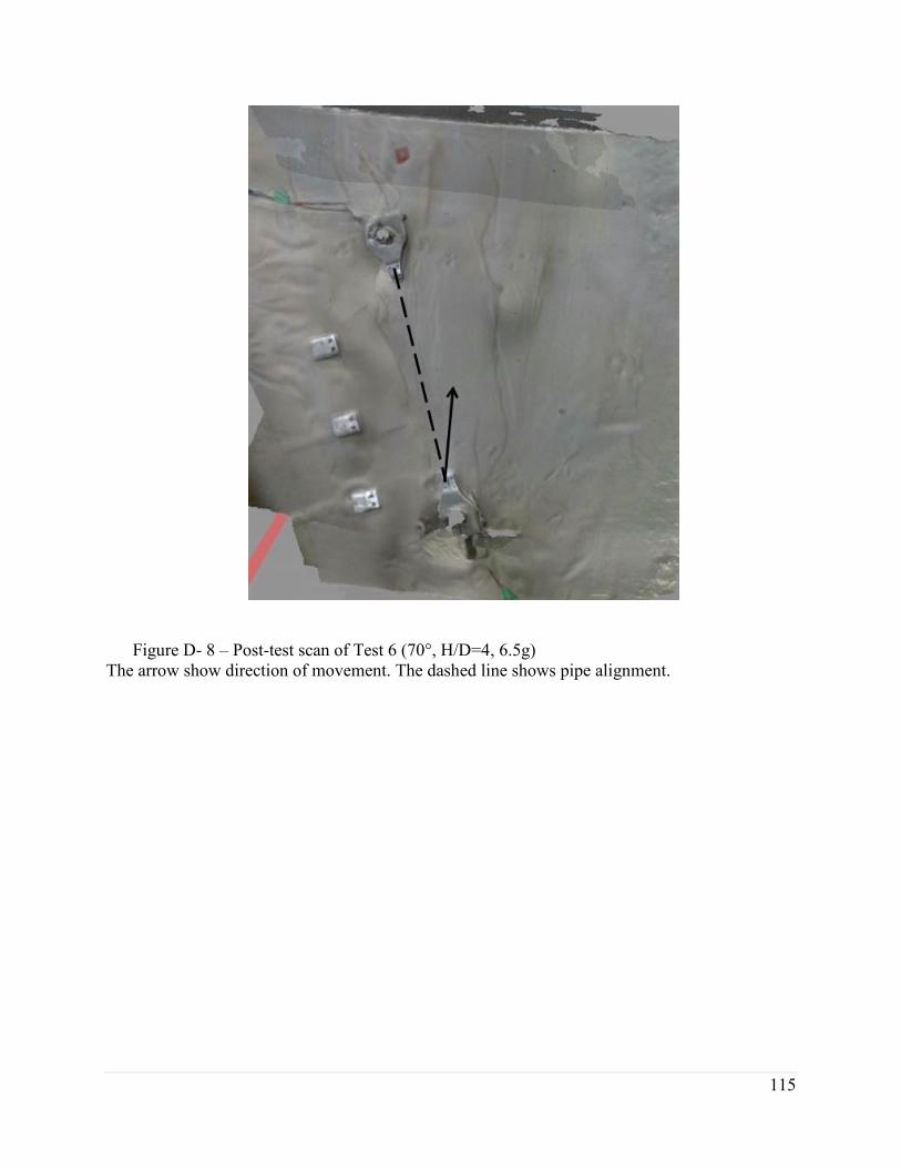
115

Figure D- 8 – Post-test scan of Test 6 (70°, H/D=4, 6.5g)

The arrow show direction of movement. The dashed line shows pipe alignment.

116

Figure D- 9 – Pre-test (right) and post-test (left) scans for Test 7 (0°, H/D=4, 13.25g)

The arrow shows the direction of movement.

117

Figure D- 10 – Pre-test (right) and Post-test (left) scans of Test 8 (20°, H/D=4, 13.25g)

The arrow shows the direction of movement.

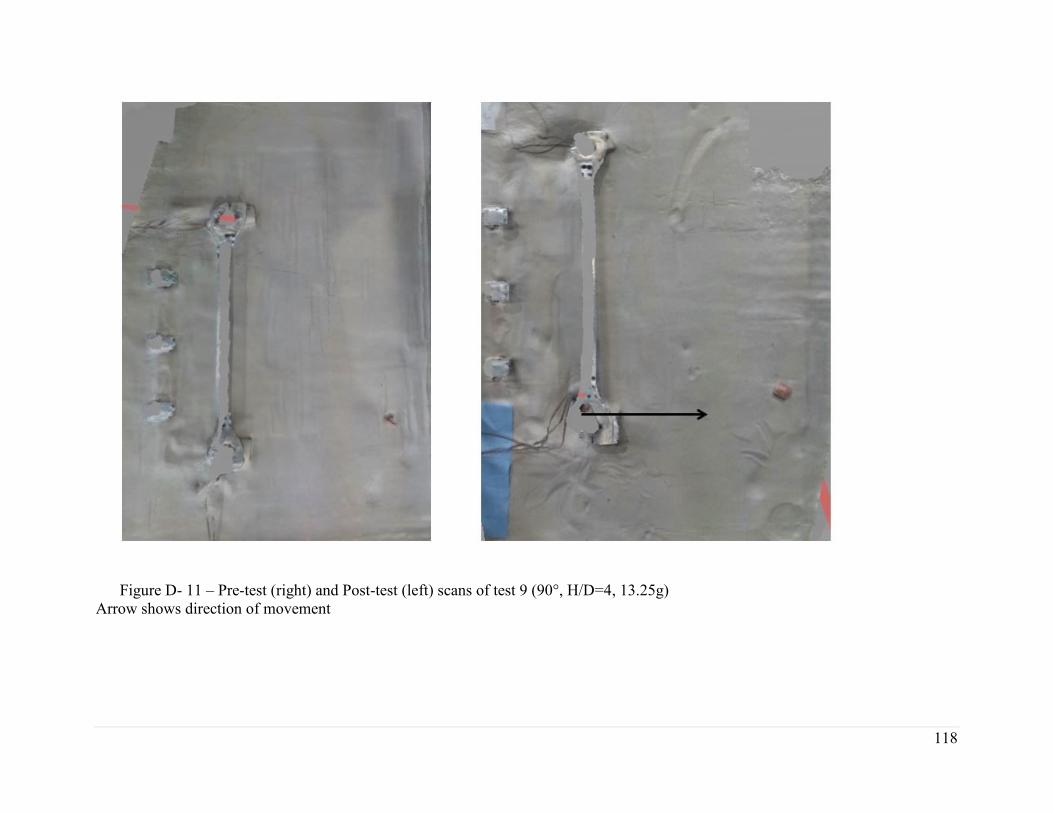
118

Figure D- 11 – Pre-test (right) and Post-test (left) scans of test 9 (90°, H/D=4, 13.25g)

Arrow shows direction of movement

119

Figure D- 12 – Pre-test (right) and Post-test scan of test 10 (30°, H/D=4, 13.25g)

The arrow shows the direction of movement.

Appendix E – Geo-Ottawa 2017 Paper

121

Centrifuge Modeling of Lateral-Axial Oblique Loading on Buried Pipelines in Cohesionless Soil G. Marcotte, S. Kenny, S. Sivathayalan Department. of Civil and Environmental Engineering, Carleton University, Ottawa, Ontario ABSTRACT Pipelines may be subject to oblique loading conditions due to relative ground motion associated with geohazards including ground subsidence, slope stability, frost heave and fault movement. Conventional guidelines for engineering stress analysis of pipe/soil interaction employ a series of orthogonal, independent springs, within structural based finite element modelling procedures, to represent soil reaction loads. This formulation cannot account for load effects during oblique pipe/soil interaction events. A series of reduced scale physical tests to investigate oblique load effects, in the lateral-axial plane, on a buried pipe in cohesionless soil were conducted in the C-CORE geotechnical centrifuge facility. A 46 mm diameter pipe was buried with a spring line cover depth of 2, and 4 pipe diameters was subject to an acceleration field of 6.25g and 13.25g, respectively. The shallow pipe modeled a 304mm pipeline and was tested at angles of 0, 20, 50, 70, and 90 degrees within lateral axial plane. The deeper pipe modeled a 609.5 mm pipeline and was tested at angles of 0, 20, 30 and 90 degrees. The imposed relative pipe/soil motion was sufficient to extend beyond peak loading conditions. A biaxial load cell measured the soil reaction loads relative to the pipe longitudinal and transverse horizontal (i.e. lateral bearing) axis. Failure surfaces for the yield load and mobilization distances were established and compared with other physical tests and numerical simulations of oblique loading events. Observations on potential scale effects in the centrifuge tests and guidance on numerical models simulating oblique loading events are discussed. RÉSUMÉ Les pipelines peuvent être soumis à des conditions de chargement obliques en raison d'un mouvement relatif du sol associé à des risques géotechnique. Les risques peuvent inclure l'affaissement au sol, la stabilité de la pente, l'accélération du gel et le mouvement des failles. Les directives conventionnelles pour l'analyse de contraintes techniques de l'interaction entre les tuyaux et les sols utilisent une série de ressorts orthogonaux et indépendants, dans les procédures de modélisation des éléments finis basés sur les structures, pour représenter les charges de réaction des sols. Cette formulation ne peut pas tenir compte des effets de charge lors d'événements d'interaction obliques entre la pipe et le sol. Une série de tests physiques à échelle réduite pour étudier les effets de charge obliques, dans le plan axial latéral, sur un tuyau enterré dans un sol sans cohésion a été réalisé dans la centrale de centrifugation géotechnique C-CORE. Un tuyau de 46 mm de diamètre a été enterré avec une profondeur de couverture de ligne de ressort de 2 et 4 diamètres de tuyaux et ont été soumis respectivement à un champ d'accélération de 6,25 g et 13,25 g. La conduite moins profonde a modelé une canalisation de 304 mm et a été testée à des angles de 0, 20, 50, 70 et 90 degrés dans le plan axial latéral. La conduite plus profonde a modelé un pipeline de 609,5 mm et a été testée à des angles de 0, 20, 30 et 90 degrés. Le mouvement relatif des conduites / sols imposé était suffisant pour s'étendre au-delà des conditions de chargement maximales. Une cellule de charge biaxiale mesurait les charges de réaction du sol par rapport à l'axe longitudinal et horizontal transversal (c'est-à-dire le roulement latéral). Les surfaces de décharge pour la charge de rendement et les distances de mobilisation ont été établies et comparées à d'autres tests physiques et des simulations numériques d'événements de chargement obliques. Les observations sur les effets potentiels de l'échelle dans les tests de centrifugation et les conseils sur les modèles numériques simulant les événements de chargement obliques sont discutées

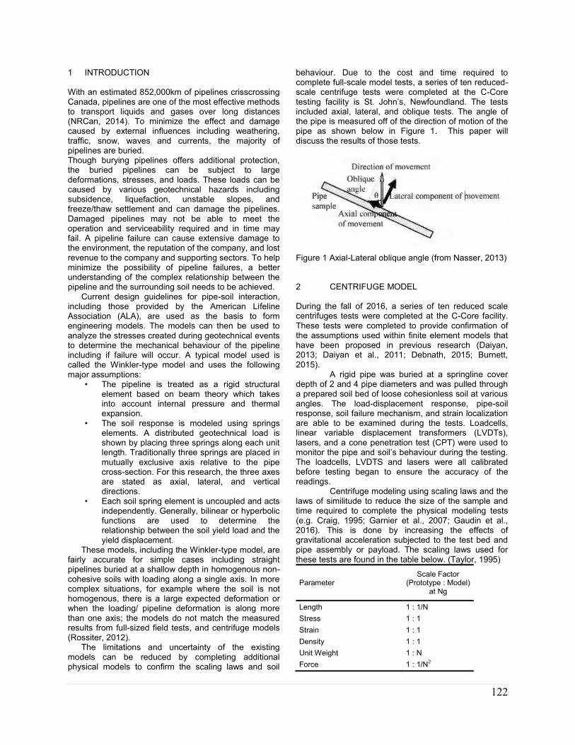
122

1 INTRODUCTION With an estimated 852,000km of pipelines crisscrossing Canada, pipelines are one of the most effective methods to transport liquids and gases over long distances (NRCan, 2014). To minimize the effect and damage caused by external influences including weathering, traffic, snow, waves and currents, the majority of pipelines are buried. Though burying pipelines offers additional protection, the buried pipelines can be subject to large deformations, stresses, and loads. These loads can be caused by various geotechnical hazards including subsidence, liquefaction, unstable slopes, and freeze/thaw settlement and can damage the pipelines. Damaged pipelines may not be able to meet the operation and serviceability required and in time may fail. A pipeline failure can cause extensive damage to the environment, the reputation of the company, and lost revenue to the company and supporting sectors. To help minimize the possibility of pipeline failures, a better understanding of the complex relationship between the pipeline and the surrounding soil needs to be achieved.

Current design guidelines for pipe-soil interaction, including those provided by the American Lifeline Association (ALA), are used as the basis to form engineering models. The models can then be used to analyze the stresses created during geotechnical events to determine the mechanical behaviour of the pipeline including if failure will occur. A typical model used is called the Winkler-type model and uses the following major assumptions:

• The pipeline is treated as a rigid structural element based on beam theory which takes into account internal pressure and thermal expansion.

• The soil response is modeled using springs elements. A distributed geotechnical load is shown by placing three springs along each unit length. Traditionally three springs are placed in mutually exclusive axis relative to the pipe cross-section. For this research, the three axes are stated as axial, lateral, and vertical directions.

• Each soil spring element is uncoupled and acts independently. Generally, bilinear or hyperbolic functions are used to determine the relationship between the soil yield load and the yield displacement.

These models, including the Winkler-type model, are fairly accurate for simple cases including straight pipelines buried at a shallow depth in homogenous non-cohesive soils with loading along a single axis. In more complex situations, for example where the soil is not homogenous, there is a large expected deformation or when the loading/ pipeline deformation is along more than one axis; the models do not match the measured results from full-sized field tests, and centrifuge models (Rossiter, 2012).

The limitations and uncertainty of the existing models can be reduced by completing additional physical models to confirm the scaling laws and soil

behaviour. Due to the cost and time required to complete full-scale model tests, a series of ten reduced- scale centrifuge tests were completed at the C-Core testing facility is St. John’s, Newfoundland. The tests included axial, lateral, and oblique tests. The angle of the pipe is measured off of the direction of motion of the pipe as shown below in Figure 1. This paper will discuss the results of those tests.

Figure 1 Axial-Lateral oblique angle (from Nasser, 2013)

2 CENTRIFUGE MODEL During the fall of 2016, a series of ten reduced scale centrifuges tests were completed at the C-Core facility. These tests were completed to provide confirmation of the assumptions used within finite element models that have been proposed in previous research (Daiyan, 2013; Daiyan et al., 2011; Debnath, 2015; Burnett, 2015). A rigid pipe was buried at a springline cover depth of 2 and 4 pipe diameters and was pulled through a prepared soil bed of loose cohesionless soil at various angles. The load-displacement response, pipe-soil response, soil failure mechanism, and strain localization are able to be examined during the tests. Loadcells, linear variable displacement transformers (LVDTs), lasers, and a cone penetration test (CPT) were used to monitor the pipe and soil’s behaviour during the testing. The loadcells, LVDTS and lasers were all calibrated before testing began to ensure the accuracy of the readings. Centrifuge modeling using scaling laws and the laws of similitude to reduce the size of the sample and time required to complete the physical modeling tests (e.g. Craig, 1995; Garnier et al., 2007; Gaudin et al., 2016). This is done by increasing the effects of gravitational acceleration subjected to the test bed and pipe assembly or payload. The scaling laws used for these tests are found in the table below. (Taylor, 1995)

Parameter Scale Factor

(Prototype : Model) at Ng

Length 1 : 1/N

Stress 1 : 1

Strain 1 : 1

Density 1 : 1

Unit Weight 1 : N

Force 1 : 1/N2

123

The sub-sections below will discuss the apparatus and testing methodology in more detail used for this set of centrifuge models. 2.1 Testing Apparatus and Instrumentation The testing apparatus and instrumentation used for this series of reduced scaled models were similar to those used by Debnath and Daiyan. As shown in Figure 2 below, the pipe assembly included a 46mm diameter hollow pipe (1) with two bi-axial loadcell (2, 3) which were used to measure the axial and lateral loads during the tests. Previous tests conducted by Daiyan used a 41mm which was heavier (Daiyan, 2013). A slightly larger, lighter pipe was used in subsequent research to minimize any downward movement of the pipe during the acceleration of the payload during testing. The pipe was pulled through the prepared soil bed by vertical stanchions (4, 5) and braced horizontally by a ‘dog bone’ piece (6). For the last two tests, which were completed at a deeper burial depth and therefore subjected to a higher load, two dog bones were used to help stiffen the assembly and to keep the stanchion in place. The two dog bone assembly (6) is shown in Figure 3 below. Two pieces of crushable acoustic foam were placed in front of the stanchions according to the direction of motion of the pipe, to limit the effect of the stanchions during pipeline mobilization. The stanchions moved into the foam during testing.

During the preparation of the soil bed, the centrepiece of the dog bone was removed, and the back bracket (7) was used to hold the pipe in place and at the correct angle. This was to ensure that the dog bone did not affect the density of the sand above the pipe during the sand raining process. Once the soil bed preparation was completed, the centrepiece of the dog bone was screwed into place, and the bracket was removed for testing. As shown in Figure 3 below, each stanchion was placed through an opening in the ball race (7, 8). The ball race acts as a sleeve for the stanchions and allows for vertical movement of the pipe assembly. The ball races are then attached to a guiding plate which is attached to the motorized carriage which is used to pull the pipe through the soil at an approximate speed of 1 mm/sec. The instrumentation used to monitor the behaviour of the soil and of the pipeline included an LVDT at each end of the dog bone (9) to monitor the vertical displacement of the pipe assembly, an LVDT in the corner of the soil bed to determine the settlement of the soil due to the acceleration of the payload, a laser to measure the horizontal displacement of the motor carriage (12), and a laser to measure the horizontal displacement of the pipe assembly. A cone (13) for a cone penetration test was also completed once the prepared sample reached the required acceleration for the test and before the mobilization of the pipe started. The CPT tests were completed to confirm that the density of the soil bed remained similar for each test.

Figure 2 Pipe assembly (1) including biaxial load cell (2, 3), stanchions (4, 5), dog bone (6), and back bracket (7).

Figure 3 Major elements of the centrifuge test apparatus (‘payload’) including dog bone (6), ball race (7, 8), LVDT (9), guiding plate (10), motorized carriage (11), laser (12), and cone (13).

2.2 Testing Methodology and Parameters

For all of the ten tests, a loose, dry test bed of fine-grained silica sand was used. Sieve analysis and direct shear box tests were completed on samples of the sand to determine their properties. As shown below in Table 1, the soil parameters used for these tests were similar to those used by Debnath for testing in loose sands (Kenny et al., 2015). All of the centrifuge tests completed by Daiyan were completed in dense, fine-grained silica sand with similar soil parameters. Direct shear tests were conducted by Marcotte (2017), and Debnath (2015). Triaxial tests were conducted by Daiyan to determine the soil parameters. Table 1 Soil test bed parameters

Parameter

Value

Marcotte (2017)

Debnath (2015)

Daiyan

(2013)

Average particle size, d50 (mm)

0.21 0.22 N/A

Peak friction angle (°) 38 40 47

Average dry density (kg/m3)

1455 1467 1598 (dense)

Relative Density (%) 32 33

82 (dense)

For all ten of the completed tests, the sand was rained into the strongbox at a constant speed from a

124

specified height. A bedding layer of 100mm (2.4D) was used for each test to ensure the bottom of the strong box did not affect the results of the test. The initial and final location of the pipe was also never closer than 2.5 D to ensure that the sides of the strong box did not affect the test results. By placing the pipe in this way, the pipe can be modeled as though it is a continuous layer of homogeneous soil.

Six tests were completed at a shallow burial depth of 2D at springline. This was the same depth that was modeled by Debnath and Daiyan. Daiyan and Debnath used an acceleration field of 12.3g and 13.25g, respectively while these tests were modeled at 6.25g (Kenny, 2015). The acceleration of 6.25g with a 46mm pipe corresponds to a pipeline that would be 304mm in diameter if a full-scale test was conducted. The shallow pipe was modeled at the following angles: 0 (pure axial), 20, 50, 70, and 90 (pure lateral) degrees within lateral axial plane. One shallow lateral test was completed with crushable foam in front of the leading stanchion, and one lateral test was completed without the crushable foam. The loadcell during the 20-degree test failed, and the axial and later yield loads were not determined.

Four tests were completed at springline burial depth of 4 pipe diameter and acceleration of 13.25g. This is the deepest that the pipe can be buried using the existing strong box. The deeper pipe modeled a 609.5 mm pipeline and was tested at angles of 0, 20, 30 and 90 degrees. Crushable foam was placed in front of the stanchions for all four of the tests. Neither Daiyan nor Debnath had completed tests at this depth. The deeper burial depth allows for a higher confining pressure on the pipe and the data obtained will be used at a later date to confirm the scaling factors and finite element analysis previously proposed.

Table 2 Centrifuge strongbox and pipe model parameters

Parameter Value

Shallow Tests Deep Tests

Acceleration field, g 6.25 13.25

Pipe diameter (mm) 41

Centrifuge strong box (mm x mm x mm)

1180 x 940 x 400

Pipe length to diameter ratio, L/D (#)

8

Pipe burial depth at springline to diameter ratio, H/D (#)

2 4

Modeled pipeline diameter (mm)

304 609.5

To help confirm the finite element models based on this series of tests, which will complete at a later date, the pipe was loaded and then unloaded several times. This cyclical loading will allow for better verification of the inputted soil properties by providing information on the elastic behaviour of the soil (Daiyan, 2013). During each test, the pipe was pulled forward for approximate 0.3 pipe diameter (0.3D) and then returned to its start position. The pipe was then moved to 0.6D,

returned to 0.3D and the mobilized to its full mobilization length. For the shallow tests, the pipe was mobilized a total of 1.0 to 1.2 pipe diameter. For the deep tests, the pipe was mobilized to a total of approximately 2.2D. The total displacement distance was determined by comparing the results of the previous research of Daiyan and Debnath and the ALA guidelines. The ultimate yield displacement proposed in the ALA guidelines is 0.1D for cohesionless soils and 0.2D for cohesive soils (Kenny and Jukes, 2015). The research previously completed determined that the ultimate yield displacement required in centrifuge testing is closer to 1 to 1.1D. With the increased confining pressure on the pipe during the deep tests, it was assumed that an increase in the overall displacement of the pipe would be required since the ultimate yield displacement was expected to be higher. The total mobilization distance was measured using the motorized carriage and confirmed with the laser measurements from the guiding plate and from the dog bone.

It should be noted that the horizontal distance measured by both lasers did not match. This was caused by the resistance of the soil on the pipe which impeded the movement of the pipe and causes a rotation of the pipe assembly. Nasser (2013) proposed a displacement correction equation of: dpipe = dguiding plate – 1.5(ddog bone –dguiding plate) This equation was based on the results of a series of in-air tests where lateral and axial loads were applied to the pipe to mimic the soil loads. The equation proposed by Nasser was deemed too conservative for the loose sand beds since the difference in horizontal measurements in the shallow tests did not exceed 5mm and did not exceed 10mm for the deep tests. A correction value of 1.1 for shallow tests and 1.25 for the deeper tests would be more accurate for the loose soil. A stiffer pipe assembly may minimize the requirements of a displacement correction equation since it would reduce the amount of rotation felt by the stanchions. 3 TEST RESULTS The real lateral and axial loads were measured using a load cell on either side of the pipe. All of the load results were normalized to ensure that they can be accurately compared to existing results. The normalized load was defined as the real force per unit length divided by the unit weight of the soil, the springline burial depth, and the pipe diameter. The real mobilization distance was divided by the pipe diameter to provide a normalized horizontal mobilization The subsections below will discuss the results of the testing completed during the fall of 2016 at the C-Core facility. The results will also be compared to existing data sets. 3.1 Axial Pipe/Soil Interaction

125

The axial test results from the deep, and the shallow tests were analyzed and compared to existing data including data from Daiyan (2013), Debnath (2015), and Hsu et al. (2001 and 2006).

The normalized axial yield force for the shallow test was 5.4N with a normalized mobilization distance of 0.1D. The normalized axial yield displacement matches the expected ALA values, but the yield force is substantially higher than specified by the ALA. As shown in the figure below, the axial yield force does fall within the range of Schaminee et al. proposed in 1990.

The normalized axial yield force for the deep test was calculated to be 23N with a normalized yield displacement of 0.15D. The yield displacement does fall within ALA’s expected values, but the yield force is substantially higher than expected. This change in values may be due to errors in assumptions used while scaling the test and to the extra confining pressure caused by the additional soil above the pipe. The pipe assembly itself including the dog bone and guiding plate deflected during testing which may have decreased the accuracy of the readings.

Figure 3 Normalized Axial Yield Displacement vs Axial Yield Force for Axial Pipe/Soil Interaction

3.2 Oblique Pipe/Soil Interaction The axial and lateral loads during the oblique and lateral tests were also measured using load cells. During the 20 degree shallow test, the loadcells failed, and the axial

and lateral yield forces were not determined. During the 30 degree deep test, the forces on the pipe assembly were too high, and the actuator was unable to mobilize the pipe to the required horizontal displacement. The yield forces were not able to be calculated for that test either. The normalized axial and lateral yield forces for the shallow tests are similar to the previous reduced scaled results. Not all of the test results fall within the pipe/soil interface failure mechanism was determined by Daiyan (2013). The pipe/soil interface mechanism requires refinement if it is to match the existing test results. Two 90 degree test were completed at the shallow depth, one with crushable foam and one without crushable foam. The crushable foam reduced the lateral loads which indicated that the foam was able to reduce the effect of the stanchions on the loadcells. All of the yield loads determined for the deep tests are higher than expected including the pure lateral and pure axial tests. This is most likely caused by the increased rotation of the pipe assembly during mobilization. The rotation created a rotational load or moment at the load cell which changes the boundary condition of the pipe. As shown in the figure below, the testing results for both the shallow and deep tests are much larger than the results of the full-scale tests completed by Hsu et al. (2001 and 2006). The tests process, testing parameters, and procedures are similar for reduced and full-scale tests, but the soil/pipe behaviour do not match. The differences in results are most likely caused by the difference in boundary conditions and axial/lateral coupling behaviour between the full and reduced scale tests. There may also be an incorrect assumption made during the scaling of the centrifuge tests. The testing results for the shallow tests are similar to the results from previous finite element simulations that have been completed by other researchers including Daiyan, 2013; Daiyan et al., 2011; Phillips et al., 2004a; Pike and Kenny, 2012a, b).

0

1

2

3

4

5

6

7

8

0 0.5 1

No

rmal

ize

d A

xial

Yie

ld F

orc

e

Normalized Axial Yield Displacement

Schaminee et al. (1990)ALA (2005)Daiyan (2013) - Dense; H/D = 2Debnath (2015) - Dense; H/D = 2Debnath (2015) - Loose; H/D = 2Hsu et al. (2001) - Loose; H/D = 1Hsu et al. (2001) - Dense; H/D = 1Marcotte (2017) - Loose; H/D = 2

126

Figure 4 Normalized Axial Yield Force vs Normalized Lateral Yield Force

4 FUTURE RESEARCH Additional research must be conducted to confirm further the assumptions made during previous finite element analysis and during previous research. The results of the full and reduced scale models still do not agree which means further research should be conducted to confirm that the correct boundary condition and scaling factors are being applied. The results from the ten tests completed this fall should also be compared to a finite element simulation to confirm that the testing procedures and parameters are accurate. The finite element simulations can also be used to confirm the axial-oblique loading coupling that seems to occur during oblique reduced-scale tests. Future reduce scaled tests should also be conducted at different burial depths and speeds. These tests can be used to further validate the scaling laws and testing procedures. Before additional reduce scaled are conducted, the pipe assembly would require reinforcement to help minimize the rotation of the stanchions during mobilization. 5 CONCLUSIONS A series of ten reduced-scale tests were completed to help confirm the assumptions used in previous research. The procedure and testing parameters used for the tests is discussed above.The shallow tests (H/D=2) results were similar to the test results of previous reduced scale oblique tests that have been completed at the C-Core facility. The deep tests (h/D=4) results were substantially higher than expected. The increase in measured loads during the deep tests was most likely caused by the rotation of the pipe assembly during loading. Further research should be conducted to confirm this and to further refine the pipeline guidelines. . 6 BIBLIOGRAPHY ALA 2005. Guidelines for the design of buried steel pipes. American Lifelines Alliance, 76p. Burnett, A. 2015. Investigation of full-scale horizontal pipe-soil interaction and large strain behaviour of sand. M.A.Sc. Thesis, Queen’sUniversity, 118p. Craig, W.H. 1995. Geotechnical centrifuge: Past, present and future. Geotechnical Centrifuge Technology, pp.1-18. Daiyan, N. 2013. InvestigatingSoil/Pipeline Interaction During Oblique Relative Movements. PhD Thesis, MemorialUniversity of Newfoundland, 204p. Daiyan, N., Kenny, S., Phillips, R. and Popescu, R. 2011. Investigating pipeline/soil interaction under axial/lateral relative movements in sand. Can. Geotech. J., 48(11): 1683-1695. Daiyan, N., Kenny, S., Phillips, R. and Popescu, R. 2010. Numerical investigation of oblique pipeline/soil interaction in sand. Proc., IPC2010-31644:6p

0

2

4

6

8

10

12

14

16

18

20

0 2 4 6 8 10

No

rmal

ize

d L

ate

ral Y

ield

Fo

rce

Normalized Axial Yield Force

Hsu et al. (2006) - Dense; H/D=2

Hsu et al. (2001) - Loose; H/D = 2

Debnath (2015) - Loose; H/D = 2

Daiyan (2013) - Dense; H/D = 2

Debnath (2015) - Loose; H/D=2

Marcotte(2017) - Loose; H/D = 2

Marcotte (2017) - Loose; H/D = 4

Pipe/Soil Interface Failure Mechanism

127

Debnath, P. 2015. Centrifuge modeling of oblique pipe/soil interaction in dense and loosesand.M.Eng. (Thesis), MemorialUniversity of Newfoundland, 120p. (in preparation) Garnier, J., Gaudin, C., Springman, S.M., et al. 2007. Catalogue of scaling laws and similitude questiosn in geotechnical centrifuge modelling. Int. J. Phy. Mod. Geo., 7(3):1-23. Gaudin, C., Randolph, M. and White, D. 2016. Centrifuge Modelling in Geotechnics. CRC Press, ISBN 9780415522243, 544p. Hsu, T.W., Chen, Y.J. and Hung, W.C.2006. Soilrestraint to oblique movement of buried pipes in dense sand." J. Transp. Eng. 132(2):175-181. Hsu, T.W., Chen, Y.J. and Hung, W.C. 2001. Soil friction restraint of oblique pipelines in loose sand. J. Transp. Eng. 127(1):82-87. Kenny, S., Jukes, P. 2015. Pipeline/Soil Interaction Modeling in Support of Pipeline Engineering Design and Integrity. John Wiley and Sons Kenny, S. Pike, K., Debnath, P., and Hawlader, B. 2015. Integrated Framework in Support of Pipeline Engineering Design for Geohazards. Geo Quebec2015 National Research Canada. 2016. 10 Key Facts on Canada’s National Resources. NRC Paulin, M. J., Phillips, R., Clark, J. I., Trigg, A., &Konuk, I. 1998.Full-scale investigation into pipeline/soil interaction. Proc., CGS:241-248. Phillips, R., Nobahar, A., and Zhou, J.2004a. Combined axial and lateral pipe-soil interaction relationships. Proc., IPC-0144:5p. Phillips, R., Nobahar, A., and Zhou, J.2004b. trench effects on pipe-soil interaction. Proc., IPC-0141:7p. Pike, K.P. and Kenny, S.P. 2012a. Lateral-axial pipe/soil interaction events: Numerical modeling trends and technical issues. Proc., IPC-90055:6p. Rossiter, C. and Kenny, S. 2012. Evaluation of lateral-vertical pipe/soil interaction in clay. Proc., OTC-23735:13p. Schaminee, P. E. L., Zorn, N. F., &Schotman, G. J. M. 1990. Soil response for pipeline upheaval buckling analyses: Full-scale laboratory tests and modelling. Proc., OTC-6486:563-572.