


Centrifugal Compressors Dynamic Considerations for · PDF fileCentrifugal Compressors Dynamic...
212
Centrifugal Compressors Dynamic Considerations for Station Design by Augusto Garcia-Hernandez Jeff Bennett Eugene L. Broerman, III Benjamin A. White, P.E. Southwest Research Institute San Antonio, Texas Presented at the 2016 Gas/Electric Partnership Houston, Texas February 2, 2016
Transcript of Centrifugal Compressors Dynamic Considerations for · PDF fileCentrifugal Compressors Dynamic...
Centrifugal Compressors Dynamic Considerations for Station Design
by Augusto Garcia-Hernandez
Jeff Bennett Eugene L. Broerman, III Benjamin A. White, P.E.
Southwest Research Institute
San Antonio, Texas
Presented at the 2016
Gas/Electric Partnership Houston, Texas February 2, 2016
Tutorial Outline
2
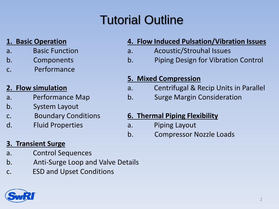
1. Basic Operation a. Basic Function b. Components c. Performance 2. Flow simulation a. Performance Map b. System Layout c. Boundary Conditions d. Fluid Properties 3. Transient Surge a. Control Sequences b. Anti-Surge Loop and Valve Details c. ESD and Upset Conditions
4. Flow Induced Pulsation/Vibration Issues a. Acoustic/Strouhal Issues b. Piping Design for Vibration Control 5. Mixed Compression a. Centrifugal & Recip Units in Parallel b. Surge Margin Consideration 6. Thermal Piping Flexibility a. Piping Layout b. Compressor Nozzle Loads

SwRI®
3
• Founded in 1947 by Thomas Baker Slick, Jr. • 501(c)(3) non-profit organization. • Broad technological base / physical sciences & engineering • Over 1,200 acre facility with over 200 buildings • Gross annual revenue of over $500 million • 2 million+ sq. ft. of laboratories & offices • Independent & unbiased • Approx. 3,000 employees • Revenue from contracts • Capital intensive operation • Internal research program
Benefiting government, industry, and the public through innovative science and technology.

SwRI Today
4
Technical Divisions Applied Physics Applied Power
Automation & Data Systems Office of Automotive Engineering
Chemistry & Chemical Engineering Defense and Intelligence Solutions
Geosciences & Engineering Mechanical Engineering
Space Science & Engineering
Southwest Research Institute®
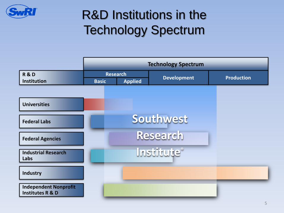
R&D Institutions in the Technology Spectrum
5
Technology Spectrum
Production Development Research
Basic Applied R & D Institution
Universities
Federal Labs
Federal Agencies
Industrial Research Labs
Industry
Independent Nonprofit Institutes R & D

Basic Operation
by Jeff Bennett
Southwest Research Institute
San Antonio, Texas
Presented at the 2016
Gas/Electric Partnership Houston, Texas February 2, 2016
1
Outline
• Discussion – Learning Objectives • Types of Centrifugal Compressors • Major Components • Working Principle • Centrifugal vs Reciprocating Compressors
2
Discussion – Learning Objectives
• What is your familiarity with centrifugal compressors?
• What are you hoping to learn?
3

Types of Centrifugal Compressors
4
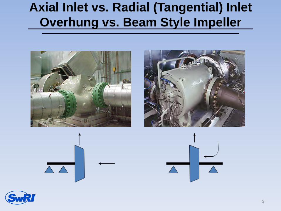
Axial Inlet vs. Radial (Tangential) Inlet Overhung vs. Beam Style Impeller
5
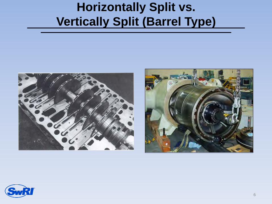
Horizontally Split vs. Vertically Split (Barrel Type)
6
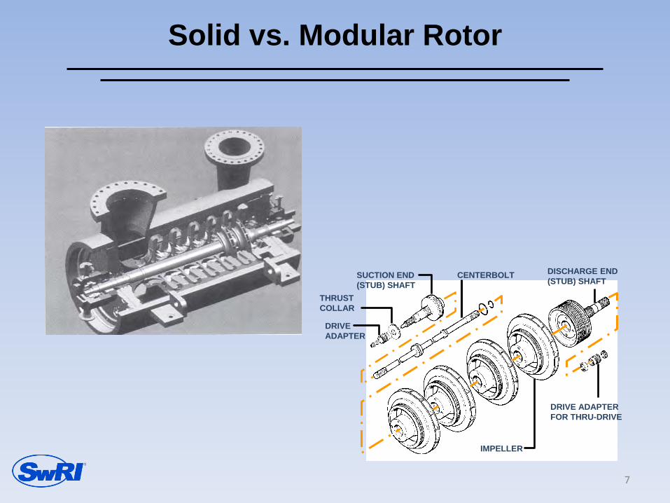
Solid vs. Modular Rotor
DRIVE ADAPTER
THRUST COLLAR
SUCTION END (STUB) SHAFT
DISCHARGE END (STUB) SHAFT
DRIVE ADAPTER FOR THRU-DRIVE
IMPELLER
CENTERBOLT
7

Straight-through vs. Back-to-back
Issues: Thrust Load (esp. transient and off-design); Interstage Leakage; Cost When: High PR, Intercooling, Sidestreams
2- body straight- through back-to-back
(Compound)
8
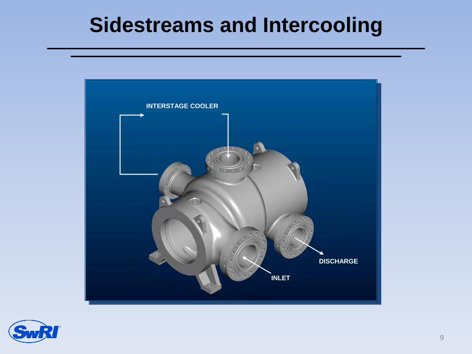
Sidestreams and Intercooling
INTERSTAGE COOLER
INLET
DISCHARGE
9

The Axial Compressor
• Airflow parallel to rotor axis • Air is compressed in “stages”
– a row of moving blades followed by a row of stationary blades (stators) is one stage.
• Moving blades impart kinetic energy
• stators recover the kinetic energy as pressure and redirect the flow to the next stage at the optimum angle
10
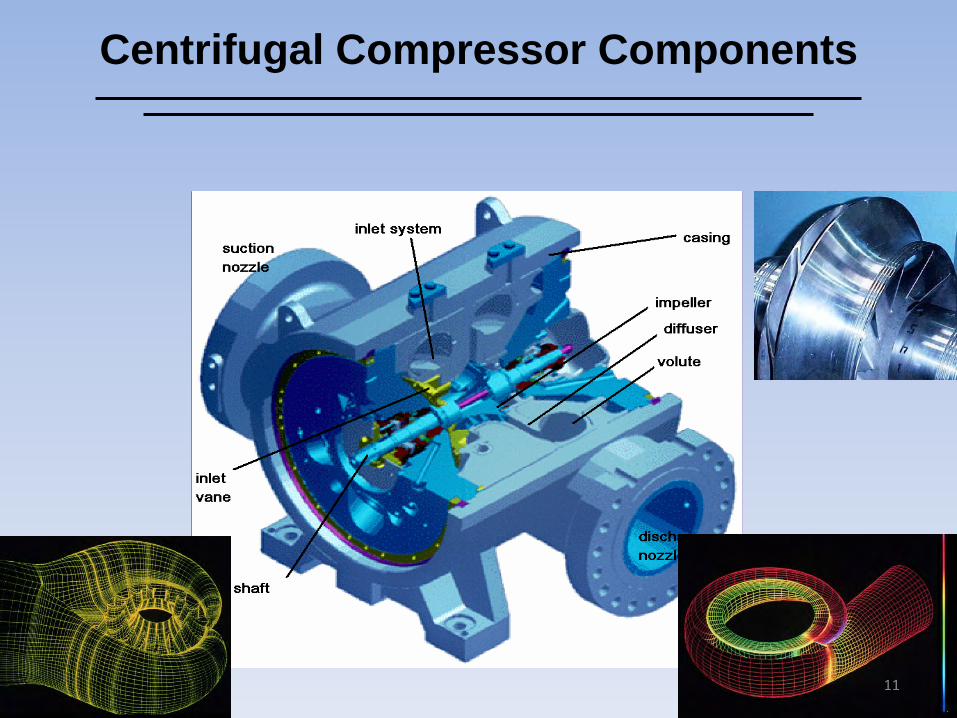
Centrifugal Compressor Components
11

Internals
12

Internals
13
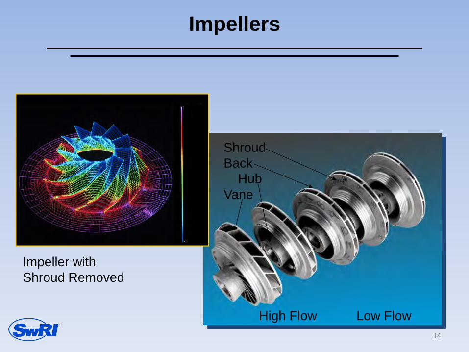
Impellers
Impeller with Shroud Removed
High Flow Low Flow
Shroud Back Hub Vane
14

Stator Components
INLET VANE
3
2 1
RETURN VANE
3 2 1
PURPOSE: To guide the flow from the inlet or the previous diffuser exit to the impeller eye of the next stage with as little losses and as uniform as possible.
15

PURPOSE: To guide the flow from the diffuser exit to the discharge nozzle with as little losses and as much pressure recovery as possible.
Volute
16

Thrust Bearings
OIL FEED GROOVE
ROTATION
THRUST COLLAR
BASE RING
THRUST PAD
OIL FEED GROOVE
THRUST PAD
ROTATION THRUST DIRECTION
LOWER LINK LEVELING DISK
(Upper Link) OIL FEED HOLE
PIVOT PIN
BASE RING
17

Journal Bearings
18
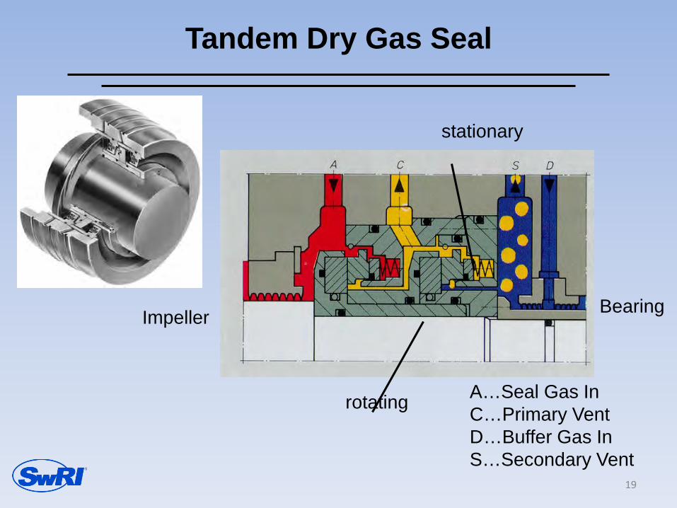
Impeller
rotating
stationary
A…Seal Gas In C…Primary Vent D…Buffer Gas In S…Secondary Vent
Bearing
Tandem Dry Gas Seal
19
The Working Principles of Centrifugal Compressors
20

Head, Work and Energy
Mechanical Work
Pressure and
Temperature Rise in the Gas
• The Compressor uses mechanical energy (‘Work’) to increase the energy of the Gas (‘Enthalpy Difference’). This energy increase is often referred to as actual head.
• The increase in energy of the gas shows as increase in pressure and temperature.
• Power is Mass Flow times Work
21

Energy
• For a flowing gas there are two types of energy involved: – Kinetic Energy (Velocity) – Potential Energy (Static Pressure)*
• They are interchangeable, i.e. static pressure can be converted into velocity and vice versa
* For completeness: ..and Elevation 22

The Three Principles
• Energy Transfer from the impeller to the fluid
• Centrifugal Force • Exchanging Pressure and Velocity
23

How Does This Apply to Gas Compression?
• The ideal compression process would increase the pressure with as little work as possible.
• Assuming a system that does not exchange heat with the ambient (‘adiabatic system’), this ideal process would not generate any losses (‘isentropic’).
24
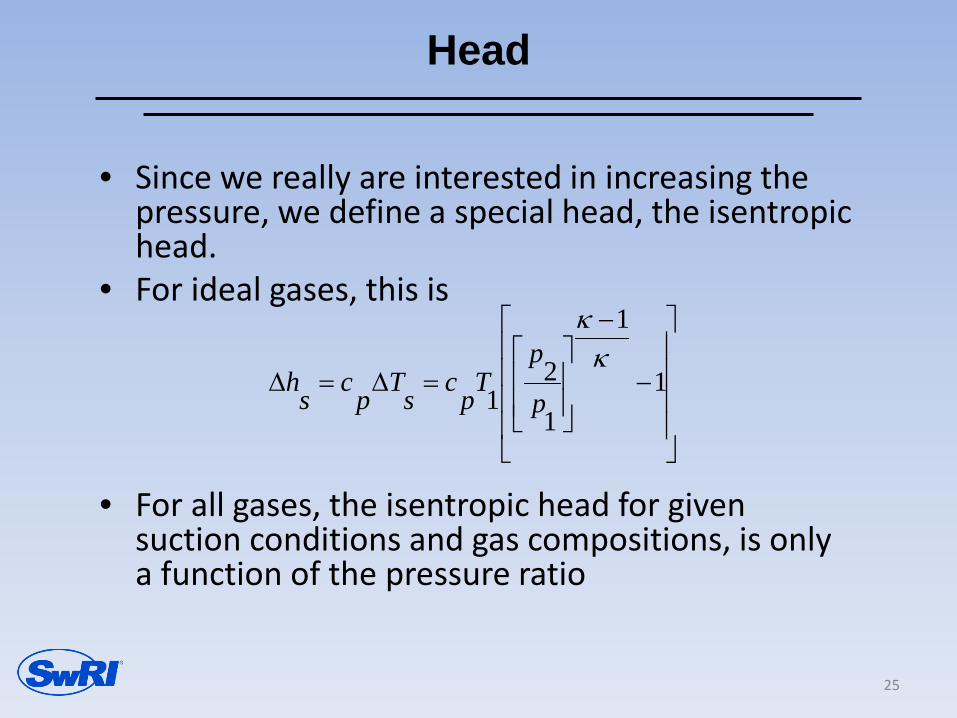
Head
• Since we really are interested in increasing the pressure, we define a special head, the isentropic head.
• For ideal gases, this is
• For all gases, the isentropic head for given
suction conditions and gas compositions, is only a function of the pressure ratio
−
−
=∆=∆ 1
1
1
21
κκ
p
pTpcsTpcsh
25

Euler for Centrifugal Machines
u1
c1 w1
u2
w2
c2
Note: The blades more or less enforce w2 and w1 The highest gas velocities are c2 and w1shroud
w2 w1
u2 u1
c2
c1
1122 ucuch uu ⋅−⋅=
The only differences from before are: - u2 is always higher than u1 - plane 1 is perpendicular to plane 2
26

After the Impeller
• Pressure and velocity are increased • We now want to convert at least some of
the velocity into pressure: • We need a diffuser
27
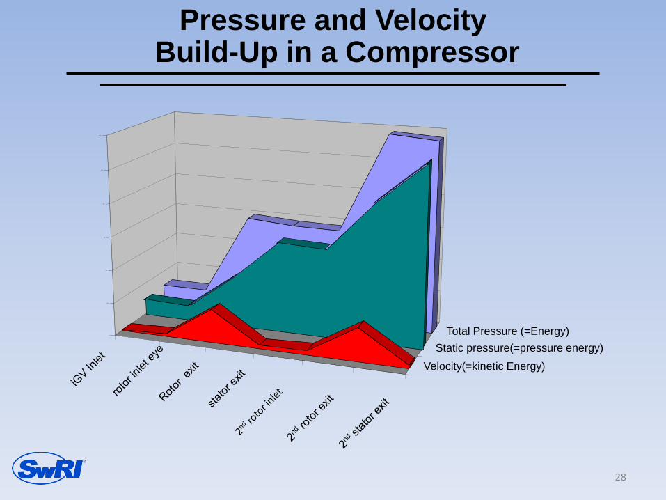
Pressure and Velocity Build-Up in a Compressor
Velocity(=kinetic Energy) Static pressure(=pressure energy)
Total Pressure (=Energy)
Total Pressure
0
200
400
600
800
1000
1200
28
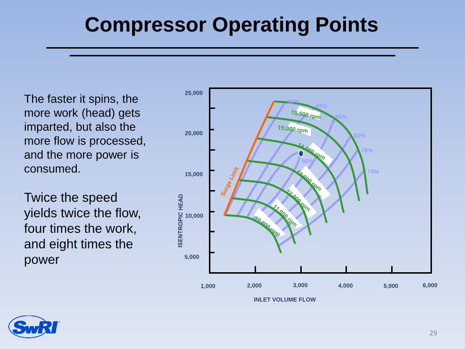
Compressor Operating Points
The faster it spins, the more work (head) gets imparted, but also the more flow is processed, and the more power is consumed. Twice the speed yields twice the flow, four times the work, and eight times the power
25,000
20,000
15,000
10,000
5,000
2,000 3,000 4,000 5,000 6,000
INLET VOLUME FLOW
74%
82%
85%
78%
85% 82%
86%
1,000
29
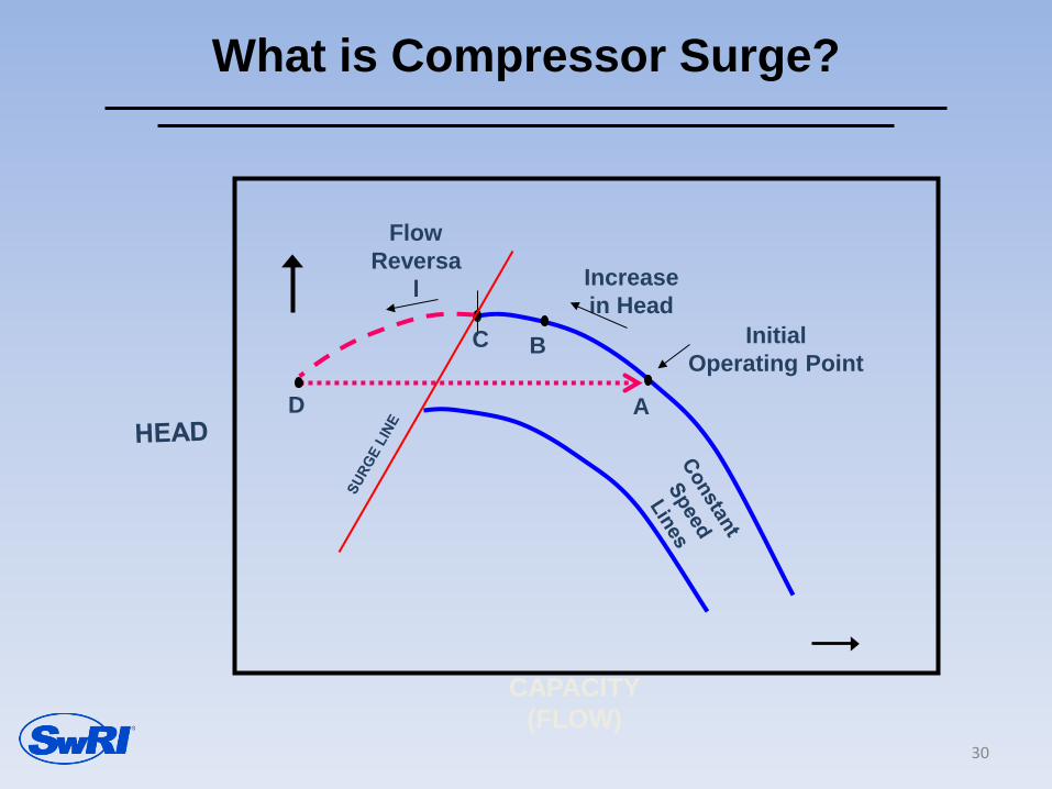
What is Compressor Surge?
CAPACITY (FLOW)
Initial Operating Point
Increase in Head
Flow Reversa
l
A
B
D
C
30
What is “Surge”?
• The point at which the impeller(s) cannot add additional work (head) to overcome the discharge pressure.
• Surge is a reversal of the entire compressor flow. It is a system behavior.
• Reversal of flow rapidly increases gas temperature into the impeller, reducing pressure ratio and aggravating surge, pressure fluctuation and rotor vibration.
• The vibration and the rapid change in axial thrust can result in damage to labyrinth seals, thrust bearings and in severe cases can also damage the rotor components and stators.
31
What is “Stall”?
• A compressor component stalls if it is operated too far away from its design point
• Stall in Centrifugal Compressors usually occurs in the diffuser, or in the inducer part of the impeller
• It often is present as rotating stall, i.e. stall cells that rotate at speeds below the running speed of the compressor
• The stall cells can induce forces into the rotor that can sometimes be detected as sub-synchronous vibrations
32
What is Choke (Stonewall)?
• The maximum flow that the compressor staging can handle at a given speed.
• Choke (or Stonewall) may occur at the impeller inlet or at the vaned diffuser inlet.
• Choke occurs because of sonic velocity or excessive negative incidence.
• All the power is dissipated in incidence and frictional losses and is a very inefficient mode of operation.
• Generally not detrimental to the Centrifugal Compressor.
33

Recip vs. Centrifugal
• The compression process in a slow running recip generates minimal losses. Losses usually occur mainly due to the gas exchange in valves, and due to pulsation dampening requirements.
• In a centrifugal, friction losses occur along the entire compression process. They are usually related to friction between the gas and the walls, or to friction between non uniform gas streams
34
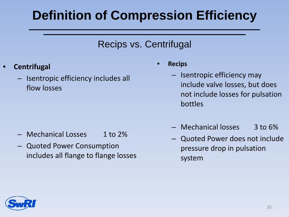
Definition of Compression Efficiency
• Centrifugal – Isentropic efficiency includes all
flow losses
– Mechanical Losses 1 to 2% – Quoted Power Consumption
includes all flange to flange losses
• Recips – Isentropic efficiency may
include valve losses, but does not include losses for pulsation bottles
– Mechanical losses 3 to 6% – Quoted Power does not include
pressure drop in pulsation system
Recips vs. Centrifugal
35

Compression Flow Modeling
by Jeff Bennett
Southwest Research Institute
San Antonio, Texas
Presented at the 2016
Gas/Electric Partnership Houston, Texas February 2, 2016
1
Outline
• Objectives and Application • Flow Modeling Levels • Modeling Process • Output Data and Analysis • Compression Network System
2

Objectives and Application
• Process flow evaluation of compression-transport systems (macro) or/and compressor units (micro)
• Typical Industry Guidelines: – API Standard 617: Axial and Centrifugal Compressors
and Expander: Basic design, performance considerations (efficiency tolerances), Annex G “ Guidelines for Anti-surge Systems”
– ANSI/ASME 31.8S: Managing System Integrity of Gas Pipelines
– GMRC - Application Guideline for Centrifugal Compressor Surge Control Systems
– Technical publications from diverse conferences
3
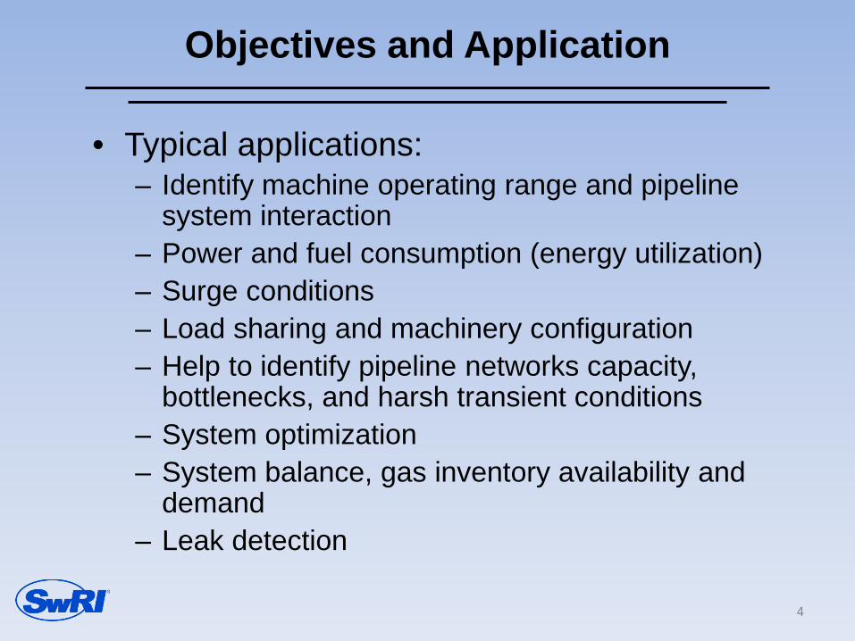
Objectives and Application
• Typical applications: – Identify machine operating range and pipeline
system interaction – Power and fuel consumption (energy utilization) – Surge conditions – Load sharing and machinery configuration – Help to identify pipeline networks capacity,
bottlenecks, and harsh transient conditions – System optimization – System balance, gas inventory availability and
demand – Leak detection
4
Flow Modeling Levels
5

Compressor Unit vs. Compression Network System
6
Level of the analysis is limited to an unit or compressor station
Compression Network System includes various compressor and regulation stations, pipeline network, injection and extraction points (customers and supplies)

Modeling Process
7
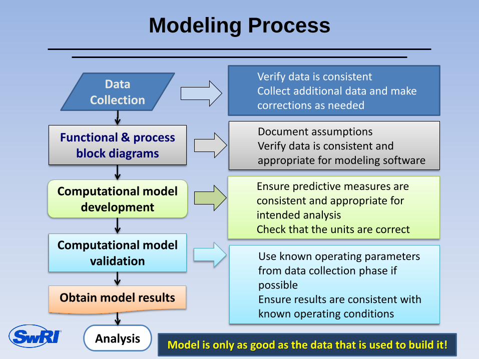
Modeling Process
8
Verify data is consistent Collect additional data and make corrections as needed
Functional & process block diagrams
Computational model development
Computational model validation
Data Collection
Obtain model results
Analysis
Document assumptions Verify data is consistent and appropriate for modeling software
Ensure predictive measures are consistent and appropriate for intended analysis Check that the units are correct
Use known operating parameters from data collection phase if possible Ensure results are consistent with known operating conditions
Model is only as good as the data that is used to build it!
Compressor Modeling
• Modeling could be performed with Excel spreadsheets or sophisticated software.
• Software selection should be based on: • Specific needs (transient solver versus steady
state) • Trained personnel • Computational time and required granularity • EOS library and compressor element • EOS used in the performance map calculations • License fees
9
Required Data Summary
• Performance compressor map • Piping layout and other equipements such as
separators/scrubbers (very specific for transient analysis, volumes), See transient modeling section
• Anti-surge system details for transient modeling • Define EOS and composition to be used in the
calculations • Operating conditions • Pipeline model of the network, if required • Define constraints and boundary conditions such as
maximum temperatures, flows, or pressure BCs
10

Model Validation and Tuning
• Validation against steady-state flows, temperature and pressure data
• Comparison of the computational model against performance compressor map, and field data if available
• Several different operating points must be evaluated
• A baseline operating condition should be used to tune the computational model
• The simulation will be run at other operating points and the results will be compared to the collected data
11

Validation and Tuning Example
Reported Values - LP
STONER - Calculated
Values
Relative Difference
(%)
Pressure (bara) 1.02 1.02 0.000Pressure (psia) 14.8 14.8 0.000Temperature (ºC) 50.3 50.3 0.000Temperature (ºF) 122.54 122.54 0.000Molecular Weight (kg/kmol) 47.3 47.3 0.000Specific Gravity (-) 1.633 1.633 0.002Compressibility (Z1) 0.985 0.985 0.000Inlet Actual Volume (m3/h) 5709 5656 0.932Inlet Actual Volume (ft3/min) 3360 3329 0.932Standard Flow (SCMH) 5207.8 5049.0 3.049Standard Flow (MMSCFD) 4.414 4.279 3.049Density (kg/m3) 1.821 1.818 0.187Density (lbm/ft3) 0.114 0.113 0.187Mass Flow Rate (kg/s) 2.89 2.86 1.117Mass Flow Rate (lbm/s) 6.37 6.30 1.117Mass Flow Rate (kg/h) 10398 10301 0.932
Pressure (bara) 4.414 4.414 0.000Pressure (psia) 64.0 64.0 0.000Temperature (ºC) 118 120.083 1.765Temperature (ºF) 244.4 248.1494 1.534Compressibility (Z2) 0.964 0.964 0.000
Polytropic Head (KJ/Kg) 89.6 89.6 0.004Polytropic Head (ft-lbf/lbm) 29975.9 29974.8 0.004Polytropic Efficiency (%) 71.8 72 0.279Speed (RPM) 10802.3 10802.3 0.000Power (Kw) 360.5 355.6 1.351Average Relative Difference - All Parameters (%) 0.435
Reported Compressor Operating Conditions
Discharge Conditions
STAGE I -LP - Point #1 PARAMETERS / COMPRESSOR
STAGE
Inlet Conditions
12

Output Data and Analysis
13

Simulations and Analysis
• Run the model to the required conditions • Perform steady and transient cases as needed • For analysis, charts and reports are very helpful:
• Plot compressor map and operating points together.
14
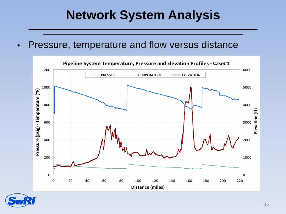
Network System Analysis
• Pressure, temperature and flow versus distance
Pipeline System Temperature, Pressure and Elevation Profiles - Case#1
0
200
400
600
800
1000
1200
0 20 40 60 80 100 120 140 160 180 200 220
Distance (miles)
Pres
sure
(psi
g) -
Tem
pera
ture
(ºF)
0
1000
2000
3000
4000
5000
6000
Elev
atio
n (f
t)
PRESSURE TEMPERATURE ELEVATION
15

Network System Analysis – Example Compression Efficiency
16

Compressor Unit Dynamic Results
• Modifications in the control sequences
0
20
40
60
80
100
120
140
2000 3000 4000 5000 6000 7000 8000 9000 10000 11000 12000
Poly
trop
ic H
ead
(kJ/
kg)
Inlet Flow (am3/hr)
Compressor Map with Different Control Sequences
Modified REV Signal Delay (0.4 sec) + No Blowdown
Modified REV Signal Delay (0.4 sec)
Earlier REV and Blowdown Opening (0.25 sec)
Real Control Sequence
7495 RPM
9636 RPM
10707 RPM
17
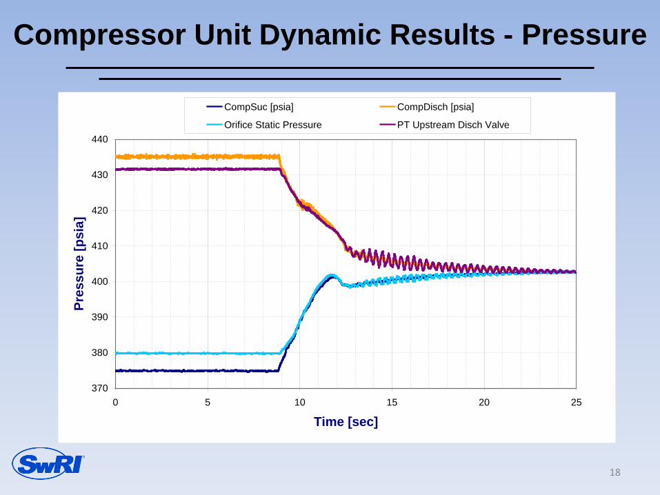
Compressor Unit Dynamic Results - Pressure
370
380
390
400
410
420
430
440
0 5 10 15 20 25
Time [sec]
Pres
sure
[psi
a]
CompSuc [psia] CompDisch [psia]
Orifice Static Pressure PT Upstream Disch Valve
18

Modeling Sensitivity Analysis
tubestubetubes
h NDUAD **4
==
After-Cooler Friction Factor
19
Compression Network System vs Compressor Station
Examples
20

Compression Network System
21
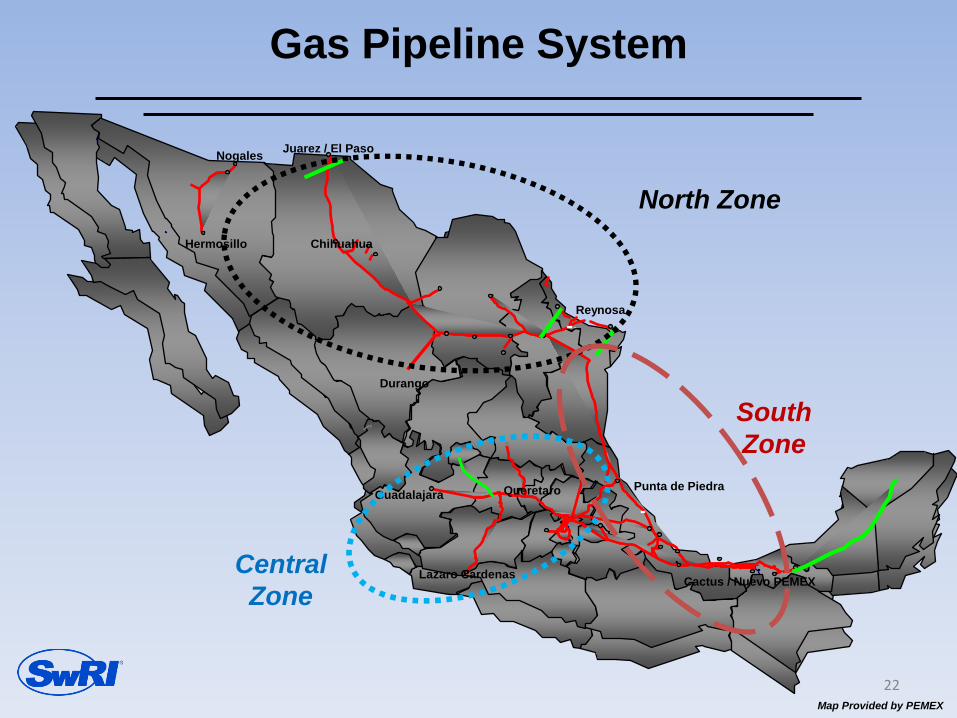
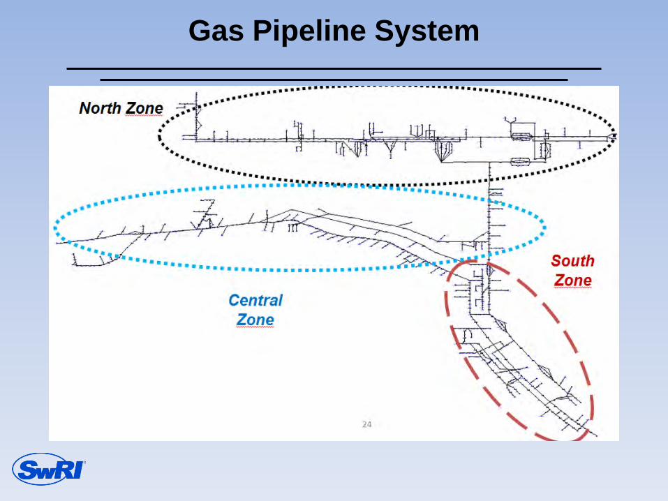
Gas Pipeline System
Nogales
Hermosillo
Juarez / El Paso
Chihuahua
Lazaro Cardenas Cactus / Nuevo PEMEX
Durango
Reynosa
Queretaro Punta de Piedra Guadalajara
Map Provided by PEMEX
North Zone
Central Zone
South Zone
22
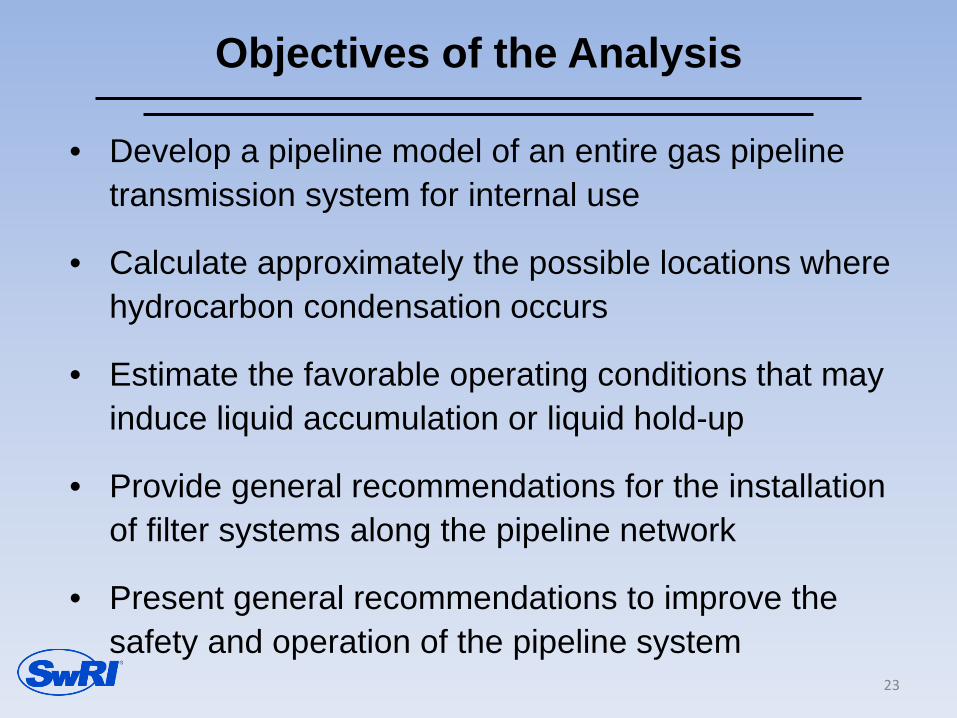
Objectives of the Analysis
• Develop a pipeline model of an entire gas pipeline transmission system for internal use
• Calculate approximately the possible locations where hydrocarbon condensation occurs
• Estimate the favorable operating conditions that may induce liquid accumulation or liquid hold-up
• Provide general recommendations for the installation of filter systems along the pipeline network
• Present general recommendations to improve the safety and operation of the pipeline system
23
Gas Pipeline System
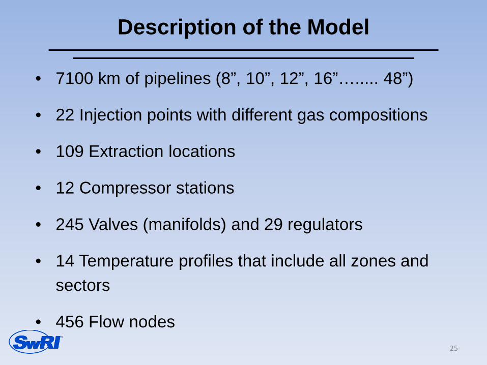
Description of the Model
• 7100 km of pipelines (8”, 10”, 12”, 16”…..... 48”)
• 22 Injection points with different gas compositions
• 109 Extraction locations
• 12 Compressor stations
• 245 Valves (manifolds) and 29 regulators
• 14 Temperature profiles that include all zones and sectors
• 456 Flow nodes 25
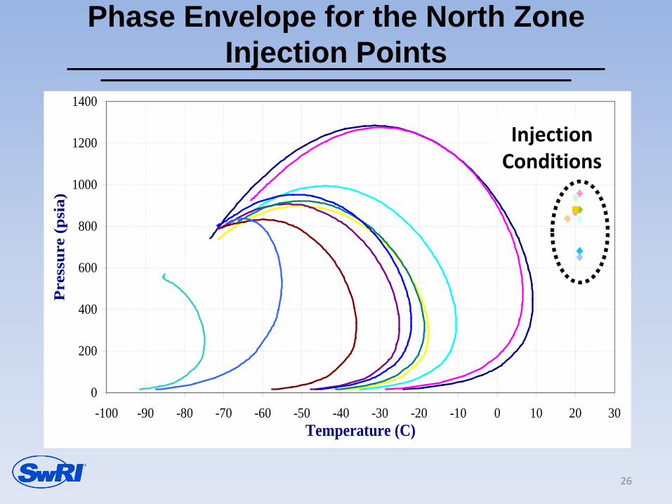
Phase Envelope for the North Zone Injection Points
0
200
400
600
800
1000
1200
1400
-100 -90 -80 -70 -60 -50 -40 -30 -20 -10 0 10 20 30Temperature (C)
Pre
ssur
e (p
sia)
Injection Conditions
26

Phase Envelop for the South Zone Injection Points
Injection Conditions
0
200
400
600
800
1000
1200
1400
1600
1800
-80 -70 -60 -50 -40 -30 -20 -10 0 10 20 30 40 50Temperature (C)
Pre
ssur
e (p
sia)
Injection Conditions
27
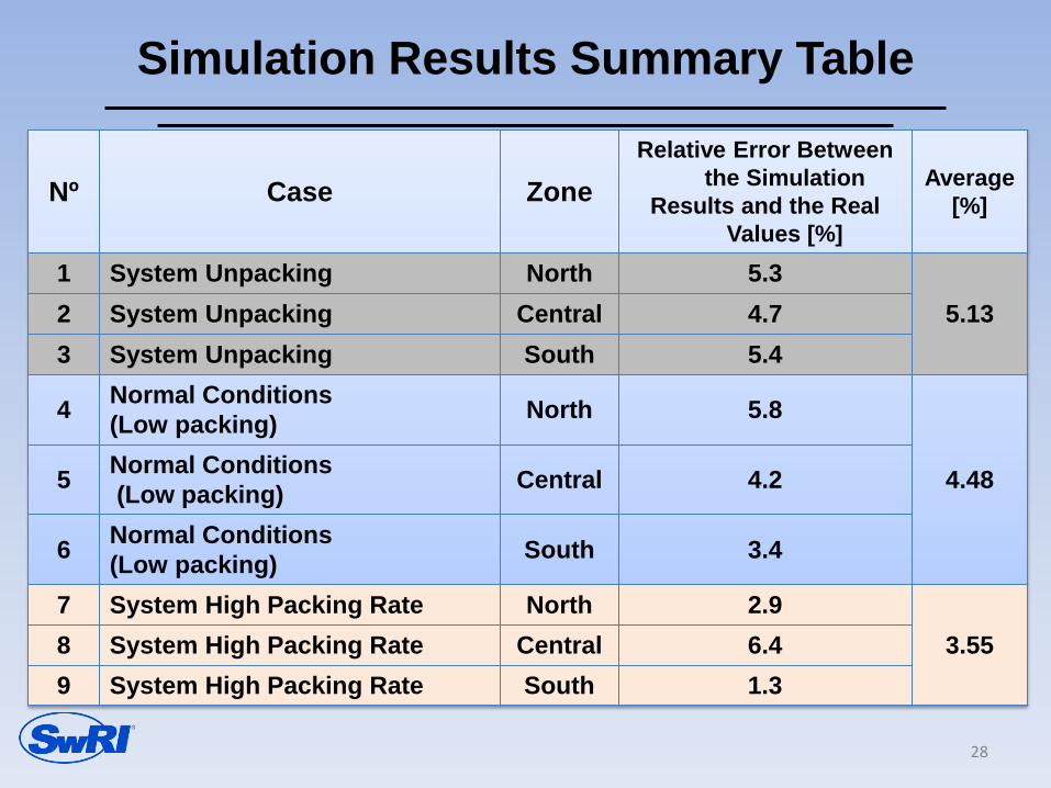
Simulation Results Summary Table
Nº Case Zone Relative Error Between
the Simulation Results and the Real
Values [%]
Average [%]
1 System Unpacking North 5.3 5.13 2 System Unpacking Central 4.7
3 System Unpacking South 5.4
4 Normal Conditions (Low packing) North 5.8
4.48 5 Normal Conditions (Low packing) Central 4.2
6 Normal Conditions (Low packing) South 3.4
7 System High Packing Rate North 2.9 3.55 8 System High Packing Rate Central 6.4
9 System High Packing Rate South 1.3
28
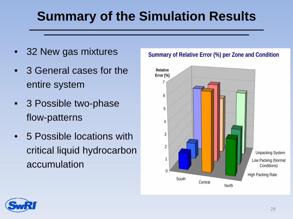
Summary of the Simulation Results
NorthCentral
South
Unpacking System
Low Packing (NormalConditions)
High Packing Rate0
1
2
3
4
5
6
7
Relative Error [%]
Summary of Relative Error (%) per Zone and Condition• 32 New gas mixtures
• 3 General cases for the entire system
• 3 Possible two-phase flow-patterns
• 5 Possible locations with critical liquid hydrocarbon accumulation
29

Transient Surge Analysis of Centrifugal Compressors
by Jeff Bennett
Augusto Garcia-Hernandez
Southwest Research Institute San Antonio, Texas Presented at the 2016
Gas/Electric Partnership Houston, Texas February 2, 2016
1

Surge
• Condition where reverse flow occurs through the compressor
• Defined as lowest flow rate for a given compressor speed
• May cause permanent damage to the compressor
2

Importance of Surge Control
An example of delayed Surge Control System response based on detection using vibration and process variables during rapid shut-down (ESD)
3
Bearing Vibration (mils)
Speed (RPM) Surge Valve Position (%Closed)
Flow Orifice Delta-P (in H20)
Surge Valve Opening Delayed by 2 Seconds
Flow Drops Rapidly
Closed
Open
Surge
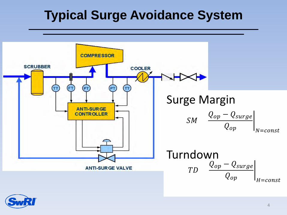
Typical Surge Avoidance System
Surge Margin Turndown
4
𝑆𝑆 =𝑄𝑜𝑜 − 𝑄𝑠𝑠𝑠𝑠𝑠
𝑄𝑜𝑜�𝑁=𝑐𝑜𝑐𝑠𝑐
𝑇𝑇 =𝑄𝑜𝑜 − 𝑄𝑠𝑠𝑠𝑠𝑠
𝑄𝑜𝑜�𝐻=𝑐𝑜𝑐𝑠𝑐
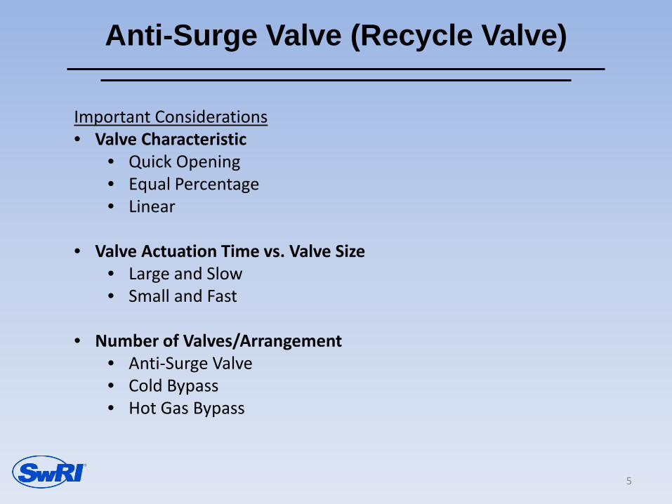
Anti-Surge Valve (Recycle Valve)
5
Important Considerations • Valve Characteristic
• Quick Opening • Equal Percentage • Linear
• Valve Actuation Time vs. Valve Size
• Large and Slow • Small and Fast
• Number of Valves/Arrangement
• Anti-Surge Valve • Cold Bypass • Hot Gas Bypass
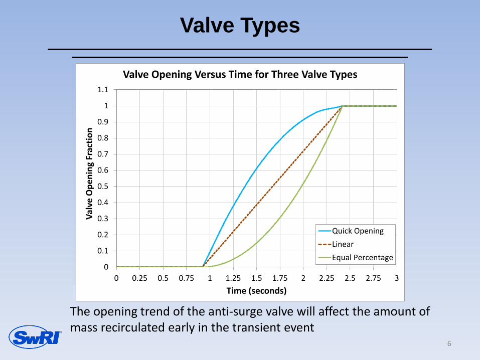
Valve Types
The opening trend of the anti-surge valve will affect the amount of mass recirculated early in the transient event
6
0
0.1
0.2
0.3
0.4
0.5
0.6
0.7
0.8
0.9
1
1.1
0 0.25 0.5 0.75 1 1.25 1.5 1.75 2 2.25 2.5 2.75 3
Valv
e O
peni
ng F
ract
ion
Time (seconds)
Valve Opening Versus Time for Three Valve Types
Quick OpeningLinearEqual Percentage
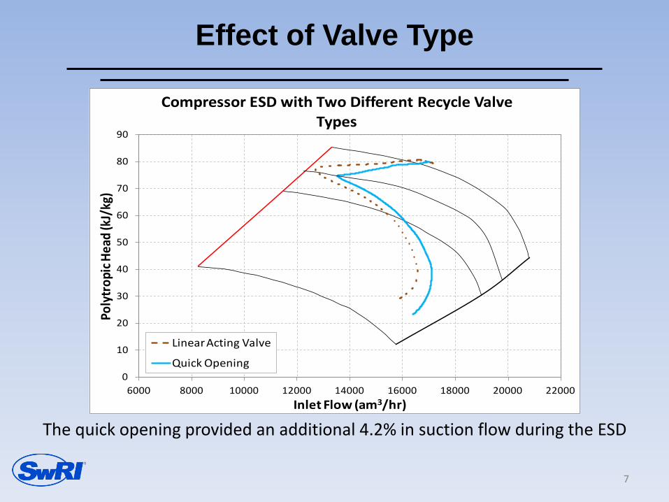
Effect of Valve Type
The quick opening provided an additional 4.2% in suction flow during the ESD
7
0
10
20
30
40
50
60
70
80
90
6000 8000 10000 12000 14000 16000 18000 20000 22000
Poly
trop
ic He
ad (k
J/kg
)
Inlet Flow (am3/hr)
Compressor ESD with Two Different Recycle Valve Types
Linear Acting Valve
Quick Opening

Valve Sizing Effect
8
0
1000
2000
3000
4000
5000
6000
7000
8000
400 500 600 700 800 900 1000 1100 1200 1300 1400 1500 1600
Isen
trop
ic H
ead
[ft-l
bf/l
bm]
Actual Flow [cfm]
Recycle Valve Sensitivity Analysis ResultsDifferent Valve Sizes opening at the same Rate
DATA SURGE LINEBase Line Modeling Modeling with +50% REV - CvModeling with +200% REV - Cv Modeling with -50%REV - Cv
19800 RPM
17800 RPM
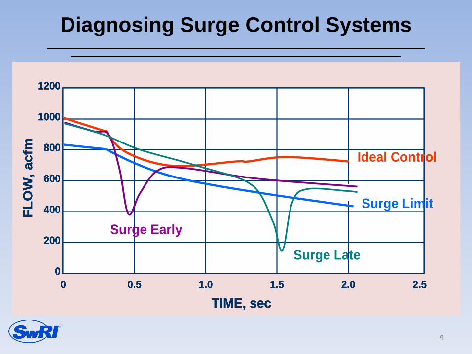
Diagnosing Surge Control Systems
9
TIME, sec2.52.01.51.00.50
1200
FLO
W, a
cfm
1000
800
600
400
200
0
Surge Limit
Ideal Control
Surge Early
Surge Late
TIME, sec2.52.01.51.00.50
1200
FLO
W, a
cfm
1000
800
600
400
200
0
TIME, sec2.52.01.51.00.50
1200
FLO
W, a
cfm
1000
800
600
400
200
0
Surge Limit
Ideal Control
Surge Early
Surge Late

Control Sequences
Small changes in the different actions’ delays will affect significantly the predictions of the system
10
0
20
40
60
80
100
120
140
2000 4000 6000 8000 10000 12000
Polyt
ropi
c Hea
d (kJ
/kg)
Inlet Flow (am3/hr)
Compressor Map with Different Control Sequences
Modified REV Signal Delay (0.4 sec) + No BlowdownModified REV Signal Delay (0.4 sec)Earlier REV and Blowdown Opening (0.25 sec)Real Control Sequence
7495 RPM
9636 RPM10707 RPM
CASE STUDY: MULTI-STAGE COMPRESSOR
11
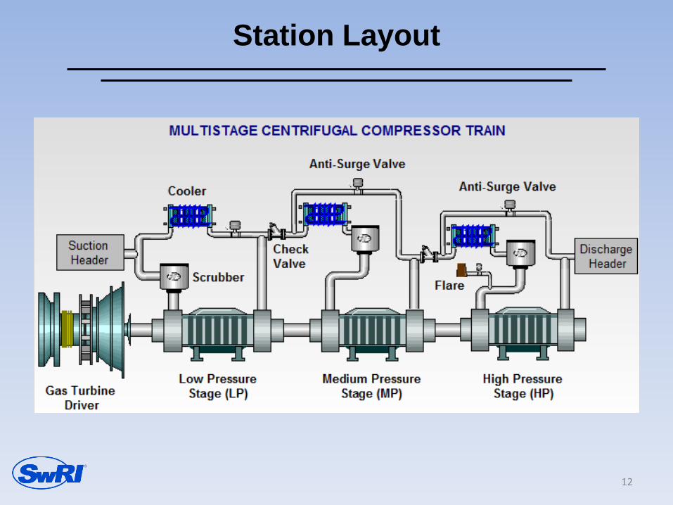
Station Layout
12
Study Goal
• Problem with low flow condition which was driving compressor to surge during emergency shutdown (ESD)
• Goal was to review existing anti-surge system design and propose changes to avoid surge during ESD from low flow conditions
13
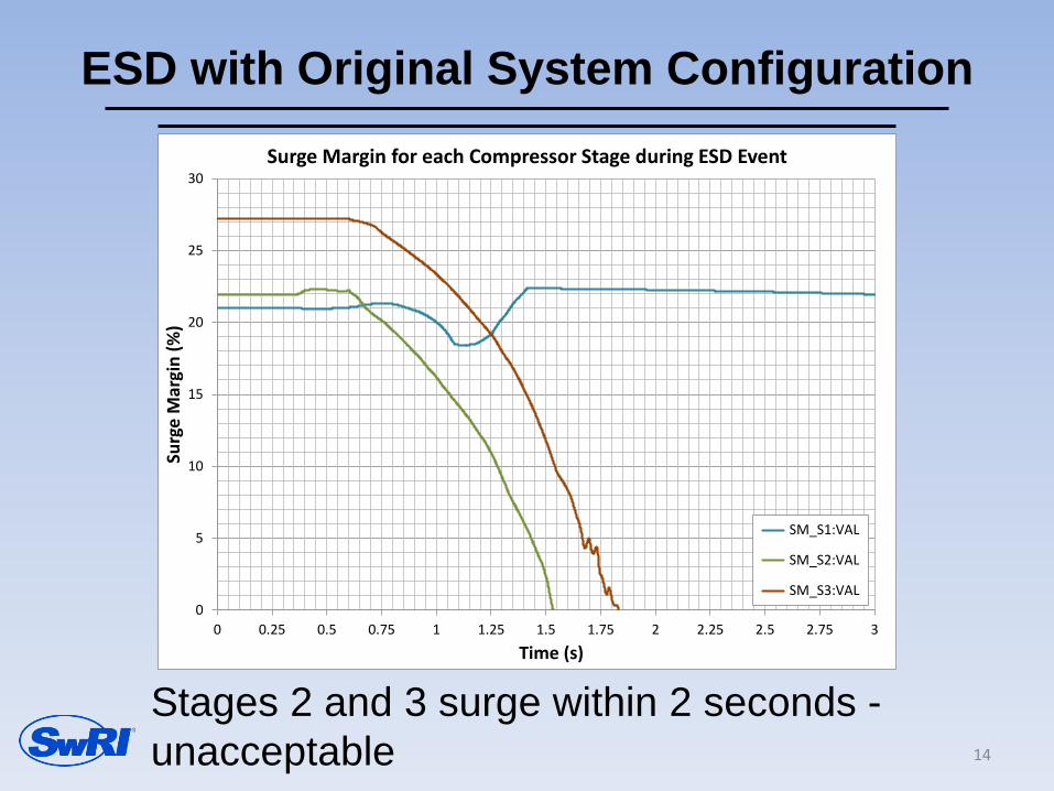
ESD with Original System Configuration
Stages 2 and 3 surge within 2 seconds - unacceptable 14
0
5
10
15
20
25
30
0 0.25 0.5 0.75 1 1.25 1.5 1.75 2 2.25 2.5 2.75 3
Surg
e M
argi
n (%
)
Time (s)
Surge Margin for each Compressor Stage during ESD Event
SM_S1:VAL
SM_S2:VAL
SM_S3:VAL

Station Modification
• Hot gas bypass added to the system plus delay coastdown
15
Suction Header
Discharge Header
Gas Turbine Driver
Low PressureStage (LP)
Medium PressureStage (MP)
igh PressureStage (HP)
Cooler
Anti-Surge Valve
Scrubber Flare
MULTISTAGE CENTRIFUGAL COMPRESSOR TRAIN
Check Valve
Anti-Surge Valve

ESD with added Hot-Bypass
• No compressor stages surge - acceptable 16
0
10
20
30
40
0 0.5 1 1.5 2 2.5 3 3.5 4
Surg
e M
argi
n (%
)
Time (s)
Surge Margin for each Compressor Stage during ESD Event with the Coast-Down Delay and Hot-Bypass
SM_S1:VAL
SM_S2:VAL
SM_S3:VAL
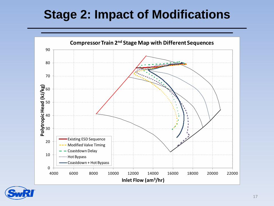
Stage 2: Impact of Modifications
17
0
10
20
30
40
50
60
70
80
90
4000 6000 8000 10000 12000 14000 16000 18000 20000 22000
Poly
trop
ic H
ead
(kJ/
kg)
Inlet Flow (am3/hr)
Compressor Train 2nd Stage Map with Different Sequences
Existing ESD SequenceModified Valve TimingCoastdown DelayHot BypassCoastdown + Hot Bypass
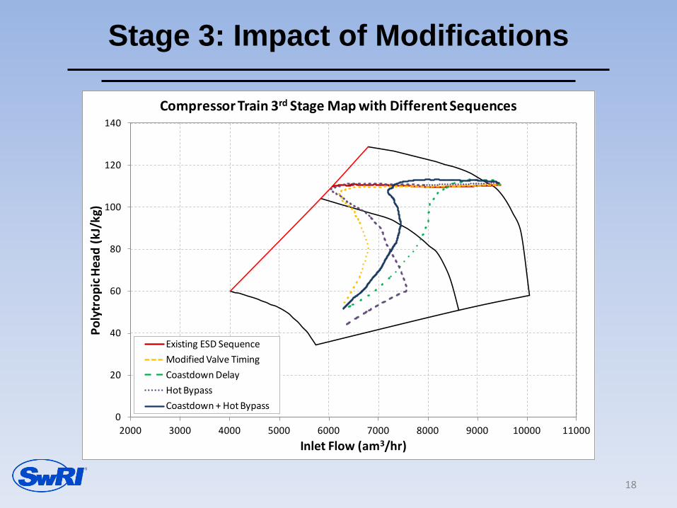
Stage 3: Impact of Modifications
18
0
20
40
60
80
100
120
140
2000 3000 4000 5000 6000 7000 8000 9000 10000 11000
Poly
trop
ic H
ead
(kJ/
kg)
Inlet Flow (am3/hr)
Compressor Train 3rd Stage Map with Different Sequences
Existing ESD SequenceModified Valve TimingCoastdown DelayHot BypassCoastdown + Hot Bypass

Summary and Conclusions (1/2)
The Five Rule of Thumbs to follow during a dynamic analysis of a centrifugal compressor:
• Rule 1- Piping Volume: impedance of the system which affects the initial dH/dQ behavior of the compressor and rate of pressure change
• Rule 2 - Recycle and Check Valves: affect system response during shutdown operation – rate of flow change and pressure
19
Summary and Conclusions (2/2)
• Rule 3 – Compressor Coastdown: very critical in the first few seconds of the ESD – deceleration rate
• Rule 4 - The Compressor Performance Map: accuracy for predicting head/flow ratio and rate of change
• Rule 5 - Control Logic: affect the sequence of events
20
Thank you for your attention!
Do you have any
questions? 21

Pulsations in Centrifugal Compressor Piping Systems
1
by Eugene L. Broerman, III
Senior Research Engineer Fluid Machinery Systems
Southwest Research Institute
San Antonio, Texas Presented at the 2016
Gas/Electric Partnership Houston, Texas February 2, 2016
Pulsation Interaction
When reciprocating compressors share common piping (typically common headers) with centrifugal compressors, pressure and flow pulsations can severely reduce the centrifugal compressor’s surge margin and operating range.
• Lateral piping of centrifugal compressor can experience
severe vibrations
• Measured pulsations could be causing centrifugal compressor performance degradation or periodic surge events
2

FLOW-INDUCED VORTEX SHEDDING IN PIPING SYSTEMS
3
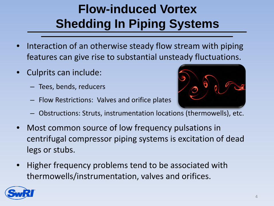
Flow-induced Vortex Shedding In Piping Systems
• Interaction of an otherwise steady flow stream with piping features can give rise to substantial unsteady fluctuations.
• Culprits can include: – Tees, bends, reducers
– Flow Restrictions: Valves and orifice plates
– Obstructions: Struts, instrumentation locations (thermowells), etc.
• Most common source of low frequency pulsations in centrifugal compressor piping systems is excitation of dead legs or stubs.
• Higher frequency problems tend to be associated with thermowells/instrumentation, valves and orifices.
4

Reynolds Number
• Flow separation and boundary layer growth are determined by fluid forces
• Flow has inertial force but viscous force retards the flow
• Reynolds number is the ratio of inertial force to viscous force
• Separation of the flow is a function of Reynolds number =Re
5
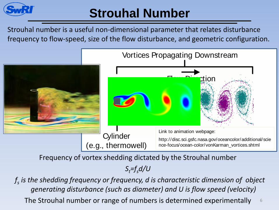
Strouhal Number
Frequency of vortex shedding dictated by the Strouhal number St=fsd/U
fs is the shedding frequency or frequency, d is characteristic dimension of object generating disturbance (such as diameter) and U is flow speed (velocity)
The Strouhal number or range of numbers is determined experimentally
Strouhal number is a useful non-dimensional parameter that relates disturbance frequency to flow-speed, size of the flow disturbance, and geometric configuration.
6
Cylinder (e.g., thermowell)
Vortices Propagating Downstream
Flow Direction
Link to animation webpage:
http://disc.sci.gsfc.nasa.gov/oceancolor/additional/science-focus/ocean-color/vonKarman_vortices.shtml
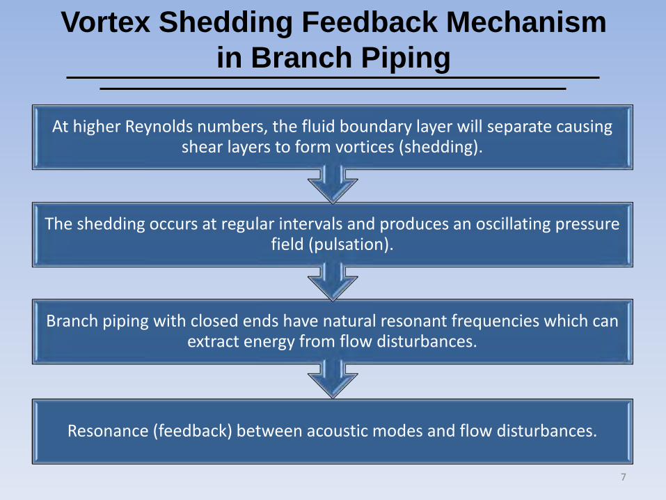
Vortex Shedding Feedback Mechanism in Branch Piping
Resonance (feedback) between acoustic modes and flow disturbances.
Branch piping with closed ends have natural resonant frequencies which can extract energy from flow disturbances.
The shedding occurs at regular intervals and produces an oscillating pressure field (pulsation).
At higher Reynolds numbers, the fluid boundary layer will separate causing shear layers to form vortices (shedding).
7
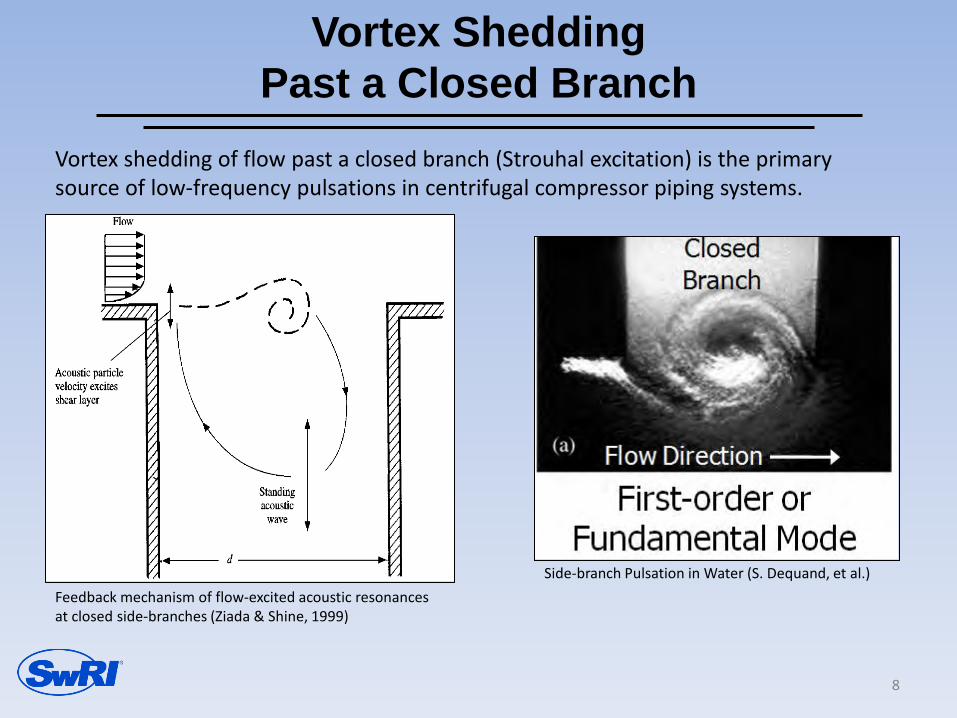
Vortex Shedding Past a Closed Branch
Feedback mechanism of flow-excited acoustic resonances at closed side-branches (Ziada & Shine, 1999)
Side-branch Pulsation in Water (S. Dequand, et al.)
Vortex shedding of flow past a closed branch (Strouhal excitation) is the primary source of low-frequency pulsations in centrifugal compressor piping systems.
8

9
ANALYSIS METHODS
Energy Institute (IE) Guideline
• Frequency avoidance method: The shedding frequency must be below the acoustic natural frequencies of the stub.
• Only works for simple stub configurations
• Does not account for the difficulty in exciting long lengths of piping (low frequencies)
• Does not account for the effects of low gas flow velocity
10

11
Graphical Comparison of Screening Methods
Vortex Shedding Screening
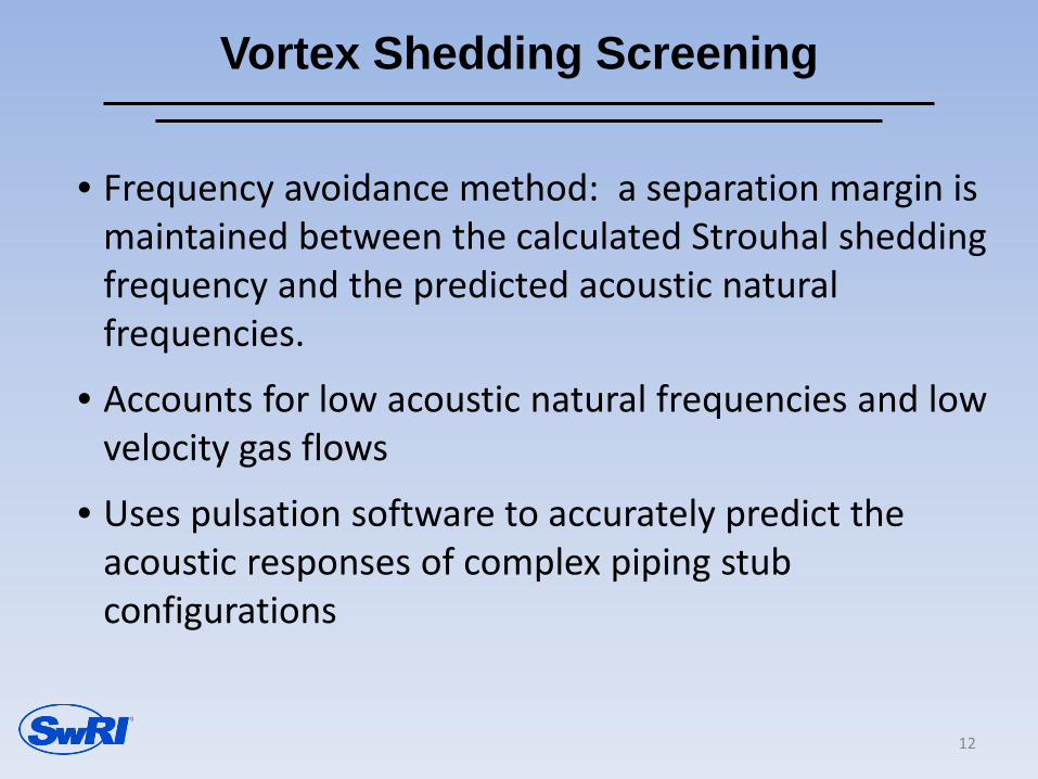
• Frequency avoidance method: a separation margin is maintained between the calculated Strouhal shedding frequency and the predicted acoustic natural frequencies.
• Accounts for low acoustic natural frequencies and low velocity gas flows
• Uses pulsation software to accurately predict the acoustic responses of complex piping stub configurations
12
Problems with Frequency Avoidance
13
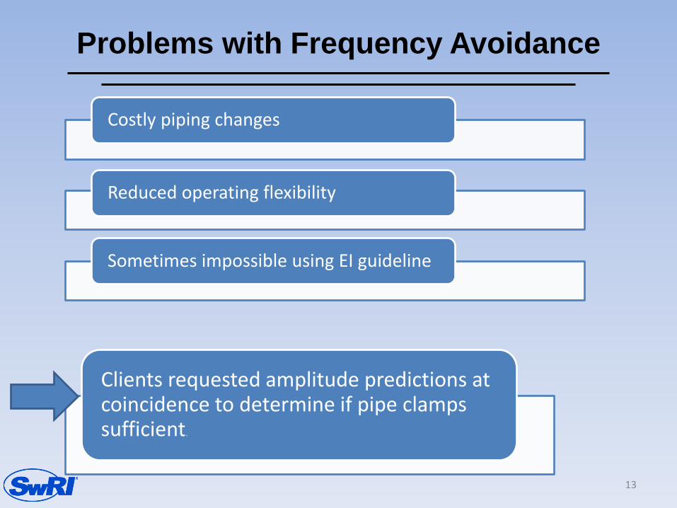
Costly piping changes
Reduced operating flexibility
Sometimes impossible using EI guideline
Clients requested amplitude predictions at coincidence to determine if pipe clamps sufficient.
Amplitude Estimation
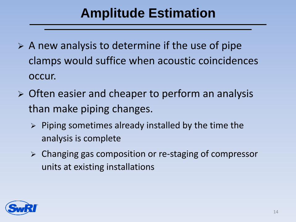
A new analysis to determine if the use of pipe clamps would suffice when acoustic coincidences occur.
Often easier and cheaper to perform an analysis than make piping changes. Piping sometimes already installed by the time the
analysis is complete Changing gas composition or re-staging of compressor
units at existing installations
14

Analysis Method Comparison
Energy Institute Guideline
Vortex-Shedding Screening
Amplitude Estimation
Requires all acoustic frequencies to be above the shedding frequency
X
Only works for very simple stubs configurations X
Coincidence avoidance method—must make piping changes if coincidence predicted
X X
Allows for a separation margin between frequencies
X X
Includes flow energy X X
Accounts for low acoustic natural frequencies (long lengths of piping)
X X
Estimates pulsation amplitudes X
Can eliminate the need for piping changes X
15

EXERCISE: CHECKING FOR A COINCIDENCE OF VORTEX SHEDDING AND ACOUSTIC
NATURAL FREQUENCIES
16
Mechanism for Excitation
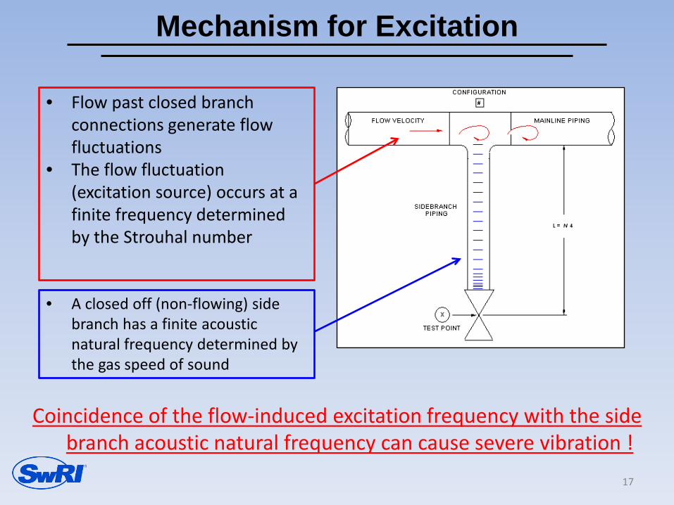
• A closed off (non-flowing) side branch has a finite acoustic natural frequency determined by the gas speed of sound
• Flow past closed branch connections generate flow fluctuations
• The flow fluctuation (excitation source) occurs at a finite frequency determined by the Strouhal number
Coincidence of the flow-induced excitation frequency with the side branch acoustic natural frequency can cause severe vibration !
17

Calculate the Acoustic Response Frequency Modes
• Side branch of 10” (9.75” I.D.) pipe with closed valve end.
• asound = Velocity of sound = 1450 ft./sec.
• Side branch supports ¼-wave “organ pipe” modes with frequencies given by:
( )
number mode 3..... 2, 1, - branch side oflength -
sound of speed - where;
412
nLa
Lanf
sound
soundn
−=
14.5 ft
V
18

19
Calculate the Vortex Shedding Frequency
• For a perpendicular side branch
• F (Hz) = 0.5 V/D, 0.5 is the Strouhal number
• Where V = Velocity (ft./sec.) = 40.625 in 24-inch main line
• And D = Branch I. D. (ft.) = 0.8125 ft (10” pipe)
• F =?? http://www.ramgen.com/tech_vortex_conventional.html
20
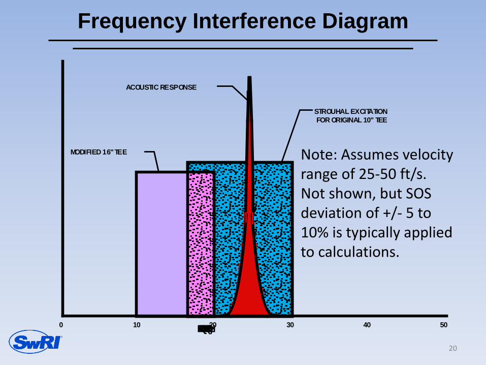
Frequency Interference Diagram
0 10 20 30 40 50
ACOUSTIC RESPONSE
MODIFIED 16" TEE
STROUHAL EXCITATION FOR ORIGINAL 10" TEE
Note: Assumes velocity range of 25-50 ft/s. Not shown, but SOS deviation of +/- 5 to 10% is typically applied to calculations.
FREQUENCY (Hz)
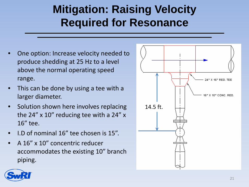
Mitigation: Raising Velocity Required for Resonance
• One option: Increase velocity needed to produce shedding at 25 Hz to a level above the normal operating speed range.
• This can be done by using a tee with a larger diameter.
• Solution shown here involves replacing the 24” x 10” reducing tee with a 24” x 16” tee.
• I.D of nominal 16” tee chosen is 15”. • A 16” x 10” concentric reducer
accommodates the existing 10” branch piping.
14.5 ft.
21

Other Possible Fixes
• Depending on the situation in question, other mitigation steps may be desirable.
• Relocate valve o Lengthens or shortens distance to
closed end of stub o Alters “organ pipe” frequency
• Increase diameter of main line
o Lowers vortex frequency o Lowers vortex energy
Vary Line Diameter?
Move Valve?
22
CASE STUDY 1: RESONANCE IN A SIDE BRANCH CAUSED BY VORTEX SHEDDING
23
24
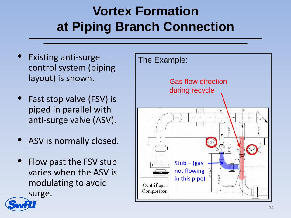
Vortex Formation at Piping Branch Connection
Gas flow direction during recycle
Stub – (gas not flowing in this pipe)
The Example: • Existing anti-surge control system (piping layout) is shown.
• Fast stop valve (FSV) is piped in parallel with anti-surge valve (ASV).
• ASV is normally closed.
• Flow past the FSV stub varies when the ASV is modulating to avoid surge.

Recycle Piping Support Damage
• During startup high vibration was observed on the second elbow downstream of the ASV/FSV piping
• Grout beneath recycle line pipe support cracking as shown
• SwRI was requested to perform field study
25
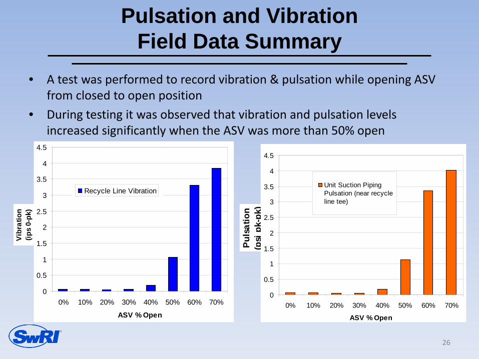
Pulsation and Vibration Field Data Summary
• A test was performed to record vibration & pulsation while opening ASV from closed to open position
• During testing it was observed that vibration and pulsation levels increased significantly when the ASV was more than 50% open
0
0.5
1
1.5
2
2.5
3
3.5
4
4.5
0% 10% 20% 30% 40% 50% 60% 70%
ASV % Open
Recycle Line Vibration
Vibr
atio
n (ip
s 0-
pk)
0
0.5
1
1.5
2
2.5
3
3.5
4
4.5
0% 10% 20% 30% 40% 50% 60% 70%
ASV % Open
Unit Suction PipingPulsation (near recycleline tee)
Puls
atio
n (p
si p
k-pk
)
26
Vortex-shedding Induced Pulsation Analysis
• Acoustical response frequencies were predicted for the FSV piping at 50 Hz (coincides with on-site field measurements).
• Corresponding Strouhal (vortex shedding) frequency was calculated at approximately 51 Hz.
• Coincidence between (excitation and ANF) = resonance = high amplitude pulsation likely.
• Conclusion: Gas flow past FSV branch connection caused vortex shedding off upstream edge of branch connection, and vortex shedding was excited an ANF, resulting in undesirable pulsation and vibration.
27
28
Modified Piping Layout Resulting from the Analyses
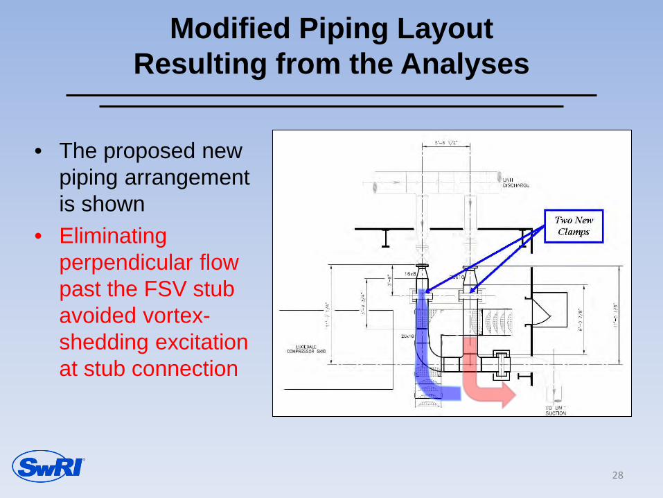
• The proposed new piping arrangement is shown
• Eliminating perpendicular flow past the FSV stub avoided vortex-shedding excitation at stub connection

Lessons Learned And Conclusions
• Acoustic/pulsation analyses are typically performed for reciprocating compressor installations, not centrifugal compressor installations since vortex shedding not addressed by most piping design codes.
• Primary lesson learned from this experience --- Coincidences of Strouhal excitation frequencies & piping ANFs could have been accurately predicted & avoided by performing an acoustic and mechanical response analysis in the piping design phase.
• Cost of piping modifications alone was approximately ten times that of typical upfront analysis.
29

QUESTIONS/COMMENTS?
30
Contact Information: Eugene ‘Buddy’ Broerman 210-522-2555 [email protected]
Sarah Simons (210) 522-2418 [email protected]

by Benjamin A. White, P.E.
Manager, R&D Fluid Machinery Systems
Southwest Research Institute
San Antonio, Texas Presented at the 2016
Gas/Electric Partnership Houston, Texas February 2, 2016
1
Piping Design for Vibration Control

Vibration in Piping and Compressor Systems
• All Piping and Compressor Systems Experience Some Vibration
• Problem When Vibration is High Enough to Cause Failures, Safety Issues, Reduce Reliability or Uncomfortable to Operators. – Vibration >>> Stress >>> Failure – Focusing on Vibration in the 0 to 200 Hz Range – Most common with Reciprocating Compressors
• Vibration Caused by: – Excessive Excitation Source (see next slide) – Mechanical Resonance – System is Too Mechanically Flexible (may or may not be
resonant) – Some Combination of the Above
2

Common Sources of Vibration in Compressor Systems (Cont’d)
• Most Common Excitation Sources – Acoustic Response (Pulsation & Shaking Forces) – Mechanical Unbalance (at the Compressor) – Gas Compression Loads (Cylinder Stretch) – Excessive Flow Velocities / Turbulence (ρv2)
• To Solve a Vibration Problem, It Is Essential to Understand the Cause(s) of the Problem. Some Problems Can Be Solved in More Than One Way – Some Must Be Solved at the Source
3
Vibrations of Complex Systems
• Complex systems have many resonant frequencies.
• For every resonant frequency, a corresponding mode shape (deflection pattern) exists.
• Vibration amplitudes are function of the force amplitude, the frequency ratio and damping.
• A system at resonance will have much higher vibration.
4

Response Of A Single Mass System
Forced Response of Mass-Spring System F(t)=F sin (2 π *freq*t)….harmonic....sinusoidal
Key Points In order to reduce response on resonance, we have several options 1 - add damping (hard) 2 - add mass (lower natural frequency) 3 - add stiffness (increase natural frequency)
Amplification Factor
ratio of excitation frequency to resonance frequency (frequency forcing / frequency natural)
0
20
40
60
80
100
120
0 0.5 1 1.5 2 2.5 3
Xk/(F
) (=
Dyn
amic
Res
p / S
tatic
Res
p)
0.0050.020.050.11
Damping Factor
On resonance, amplification factor is controlled by damping
Note: In many piping systems, damping will range from 1% to 2% (Q = 25 to 50).
mk /2
1nseFreq_Respoπ⋅
=
5
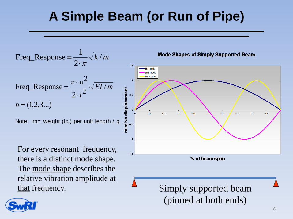
A Simple Beam (or Run of Pipe)
mk /2
1nseFreq_Respoπ⋅
=
For every resonant frequency, there is a distinct mode shape. The mode shape describes the relative vibration amplitude at that frequency. Simply supported beam
(pinned at both ends)
...)3,2,1(
/22
2nnseFreq_Respo
=⋅
⋅=
n
mEIl
π
Note: m= weight (lbf) per unit length / g
6
Piping Design for Vibration Control
Main Factors in Piping Design for Vibration Control • Restraint Locations • Restraint Types
• Excitation Source (Pulsation Amplitudes & Frequencies)
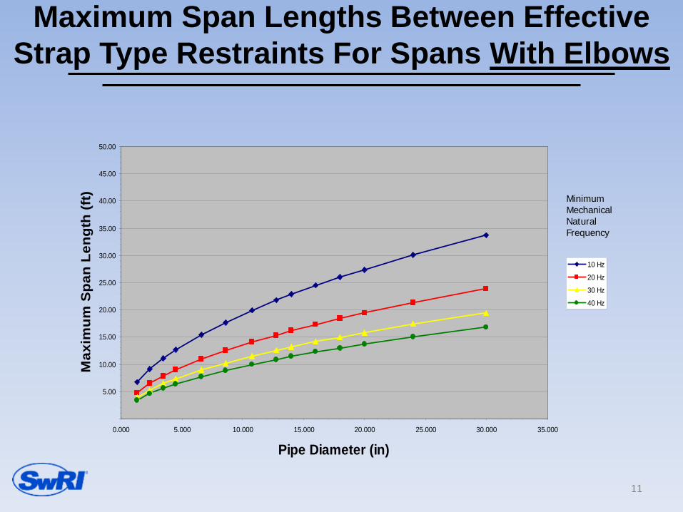
• Maximize Mechanical Natural Frequencies (Place Above Excitation Frequencies).
• API 618 Minimum MNF = 2.4 * Running Speed/60 • 10 Hz for Centrifugal Units
7

Typical Piping Configurations
• 1st column shows various simple piping layouts.
• 2nd column shows the deflection pattern of lowest mechanical natural frequency.
• Which points have the greatest deflections?
8
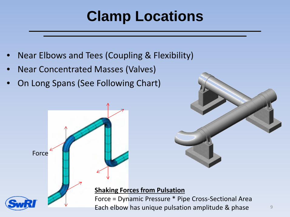
Clamp Locations
• Near Elbows and Tees (Coupling & Flexibility) • Near Concentrated Masses (Valves) • On Long Spans (See Following Chart)
Shaking Forces from Pulsation Force = Dynamic Pressure * Pipe Cross-Sectional Area Each elbow has unique pulsation amplitude & phase
Force
9
5.00
10.00
15.00
20.00
25.00
30.00
35.00
40.00
45.00
50.00
0.000 5.000 10.000 15.000 20.000 25.000 30.000 35.000
Pipe Diameter (in)
Max
imum
Spa
n Le
ngth
(ft)
10 Hz
20 Hz
30 Hz
40 Hz
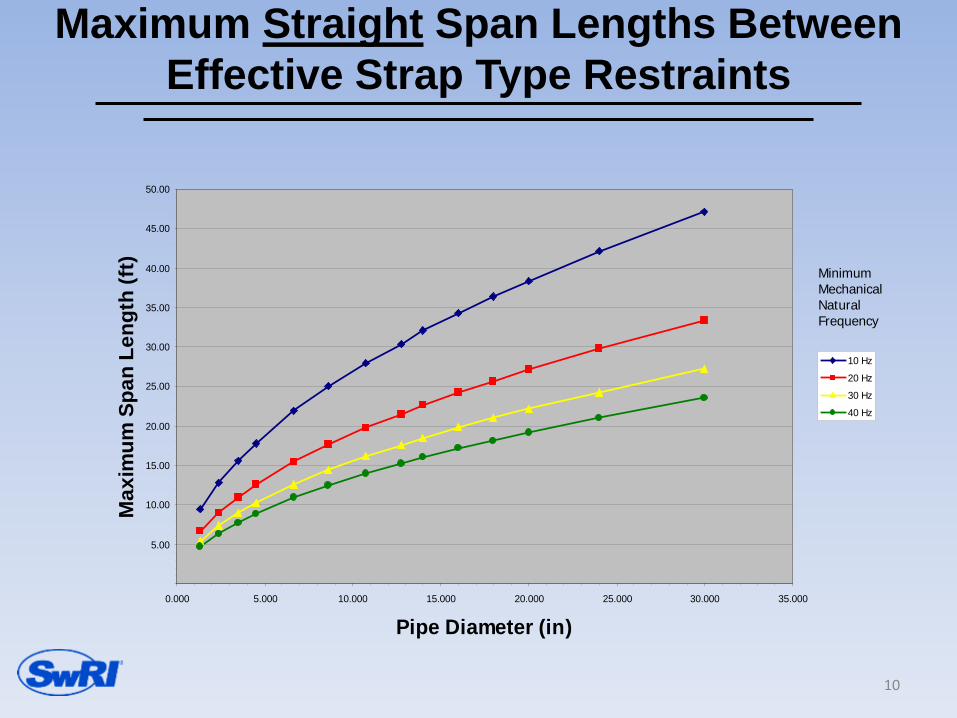
Maximum Straight Span Lengths Between Effective Strap Type Restraints
Minimum Mechanical Natural Frequency
10
5.00
10.00
15.00
20.00
25.00
30.00
35.00
40.00
45.00
50.00
0.000 5.000 10.000 15.000 20.000 25.000 30.000 35.000
Pipe Diameter (in)
Max
imum
Spa
n Le
ngth
(ft)
10 Hz
20 Hz
30 Hz
40 Hz
Maximum Span Lengths Between Effective Strap Type Restraints For Spans With Elbows
Minimum Mechanical Natural Frequency
11

Piping Layout Issues #1
• Avoid Unsupported Overhanging Elbows.
• Avoid Unsupported Weights (Valves, Flanges, etc).
Poor Layout Without Support Near Elbow and Flange.
12

Piping Layout Issues #2
Good Layout: • Minimize Elbows • Minimize Elevated Piping
Poor Layout: • Too Many Elbows (Too Flexible) • Elevated (Difficult to Support)
13
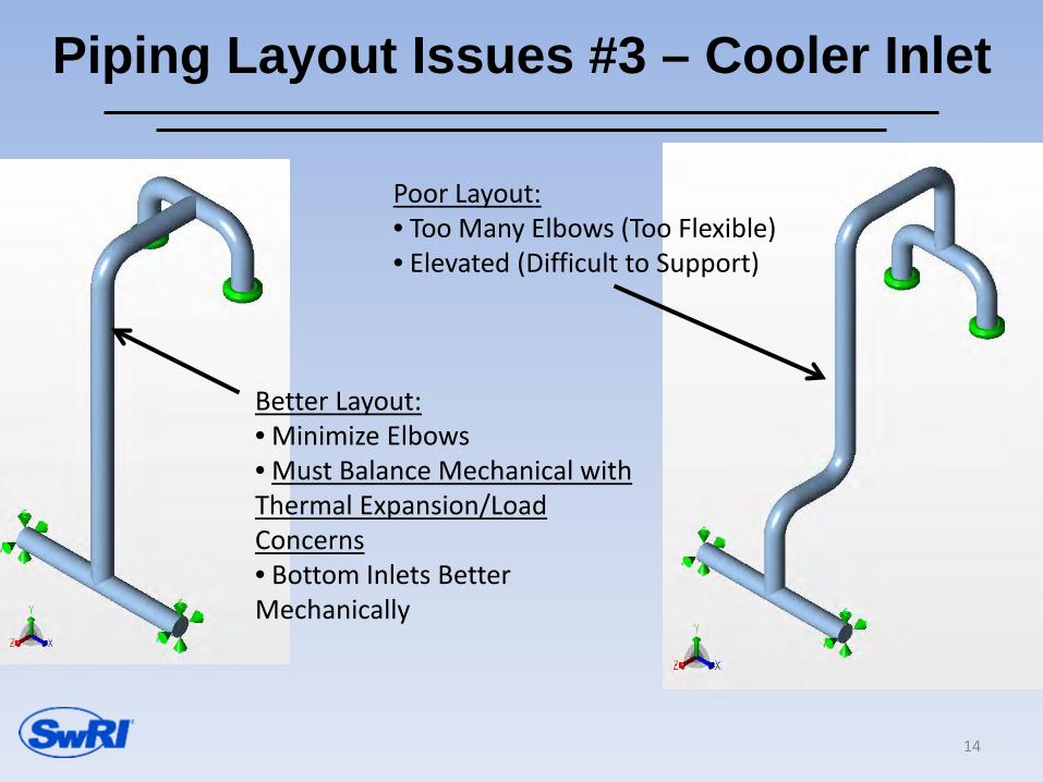
Piping Layout Issues #3 – Cooler Inlet
Better Layout: • Minimize Elbows • Must Balance Mechanical with Thermal Expansion/Load Concerns • Bottom Inlets Better Mechanically
Poor Layout: • Too Many Elbows (Too Flexible) • Elevated (Difficult to Support)
14

Restraint Types And Stiffness
• Different Restraints Have Different Stiffness Properties • Simple Weight Supports • Guides, Stops, Spring Cans and Hangers • Box Clamps • U-bolts • Strap Type Hold-down Clamps (With Or Without
Wedges) Are Best For Vibration Control. • For Accurate Modeling Predictions, It Is Essential to
Accurately Estimate Stiffness in All Directions
15

Effective Clamping
Clamp Characteristics • Adequate Plate Thickness • Side Gussets • ½ Inch Gap Between Clamp & Structure • Adequate Number and Size of Bolts • Clamp Liner Material • Clamp Should Be Several Times Stiffer Than Pipe • Attached Structure Must Be Adequately Stiff
1/8” thick fabric-pad Belting material bonded
to clamp surface
Gusset Plates
Bolts (double nut)
16

Poor Clamping
Loose pipe strap – Liner (i.e., Fabreeka) between clamp and bottle is free to move
Pipe strap with no bolt gap
Not Built as Designed
17

Poor Clamping #2
18

Flexible Structure Under Clamp
Excessive Gap
Stretch Tube Design (good and bad)
Poor Clamping #3
19
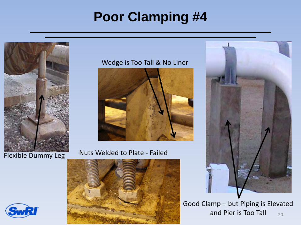
Poor Clamping #4
Wedge is Too Tall & No Liner
Good Clamp – but Piping is Elevated and Pier is Too Tall
Nuts Welded to Plate - Failed Flexible Dummy Leg
20
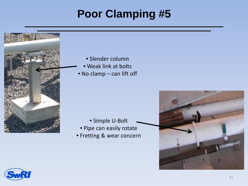
Poor Clamping #5
• Slender column • Weak link at bolts
• No clamp – can lift off
• Simple U-Bolt • Pipe can easily rotate
• Fretting & wear concern
21
Clamp Installation And Maintenance
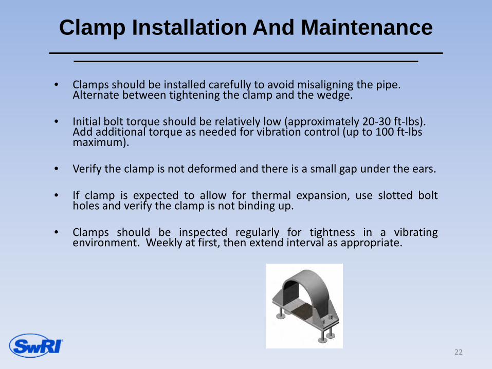
• Clamps should be installed carefully to avoid misaligning the pipe. Alternate between tightening the clamp and the wedge.
• Initial bolt torque should be relatively low (approximately 20-30 ft-lbs). Add additional torque as needed for vibration control (up to 100 ft-lbs maximum).
• Verify the clamp is not deformed and there is a small gap under the ears.
• If clamp is expected to allow for thermal expansion, use slotted bolt holes and verify the clamp is not binding up.
• Clamps should be inspected regularly for tightness in a vibrating
environment. Weekly at first, then extend interval as appropriate.
22

Small Bore Branch Connection Piping
• Small diameter connections are highly susceptible to vibration & fatigue.
• Very common problem area – usually no formal analysis.
• Even low vibration amplitude on mainline can excite significant branch vibration.
23

Small Bore Branch Connection Piping
• Keep attachments short and stiff.
• Sch 80 pipe minimum & good welding.
• Minimize large overhanging mass on small flexible line.
• Support branch line back to mainline (thermal concerns).
• Avoid fittings with high stress concentration factors (threads, etc.) in high vibration environments.
• Pads, saddles, tees, etc. can be used in critical applications.
• GMRC and Energy Institute Guidelines
24 GMRC - Design Guideline for Small Diameter Branch Connections (2011). Energy Institute - Guidelines for the Avoidance of Vibration Induced Fatigue Failure in Process Pipework (2008).
Summary of Good Practices for Controlling Piping Vibration
• Use good dynamic piping restraints (high stiffness) with proper fabrication, installation & maintenance.
• Locate clamps near elbows, tees, and concentrated masses.
• Good support structures attached to clamps. • Avoid excessive elbows and elevated piping. • Brace auxiliary piping (minimize cantilevered masses).
25

Allowable Vibration Limits
• Piping fatigue failure caused by excessive stress – NOT by excessive vibration amplitude.
• Stress and vibration amplitude are related, but the relationship is different for each piping configuration.
• Displacement is often used for screening measured vibration since it is easy to measure.
• A more flexible system can have higher vibration with lower stress. • However, high vibration should be avoided (even if stress levels are
acceptable) since vibration can cause other problems: – Increased maintenance / bolts loosening – Operator discomfort – Problems with attached instrumentation, etc.
26
Allowable Vibration Limits
Because vibration is easy to measure, several guidelines exist: • SwRI Screening Piping Vibration Severity Chart (covered
later) • EFRC Guideline (European Forum on Reciprocating
Compressors) • OEM Equipment Guidelines • Various API & ISO Standards such as:
– API 618 – Reciprocating Compressors – ISO 10816-6
• Most piping codes (B31.3, B31.8, etc) very minimal guidance.
• Wide range of standards and approaches that don’t always agree.
27
SWRI RECOMMENDED SCREENING PIPING
VIBRATION SEVERITY CHART
(Vibration Displacement vs. Frequency)
28
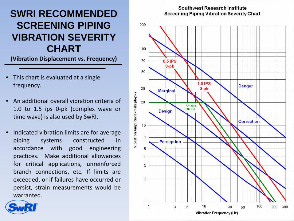
• This chart is evaluated at a single frequency.
• An additional overall vibration criteria of 1.0 to 1.5 ips 0-pk (complex wave or time wave) is also used by SwRI.
• Indicated vibration limits are for average piping systems constructed in accordance with good engineering practices. Make additional allowances for critical applications, unreinforced branch connections, etc. If limits are exceeded, or if failures have occurred or persist, strain measurements would be warranted.

QUESTIONS?
29
Benjamin A. White, P.E. Contact info: Southwest Research Institute Tel: 210-522-2554 [email protected]
GEP Short Course – Mixed Compression
by Eugene L. Broerman, III
Senior Research Engineer Fluid Machinery Systems
Southwest Research Institute
San Antonio, Texas Presented at the 2016
Gas/Electric Partnership Houston, Texas February 2, 2016
1

Effect of Inlet Pulsations and Piping Acoustic Impedance on Centrifugal Compressor Surge
2
Overview
• Many compressor stations have both recip and centrifugal compressors installed.
• There is still limited understanding of how pulsations, piping resonance, and impedance impact centrifugal compressor performance and surge.
• The compressor map does not provide a complete picture on how the compressor will respond to rapid transients (pulsations) and how its surge margin is affected due to lack of knowledge and data.
• Fundamental questions: – Can pulsations drive a centrifugal compressor into surge? – If so, what amplitudes and frequencies are required? – How does pipe impedance impact pulses (amplification/attentuation)?
Unexpected periodic surge has been observed in the compressors when pulsations were present.
3
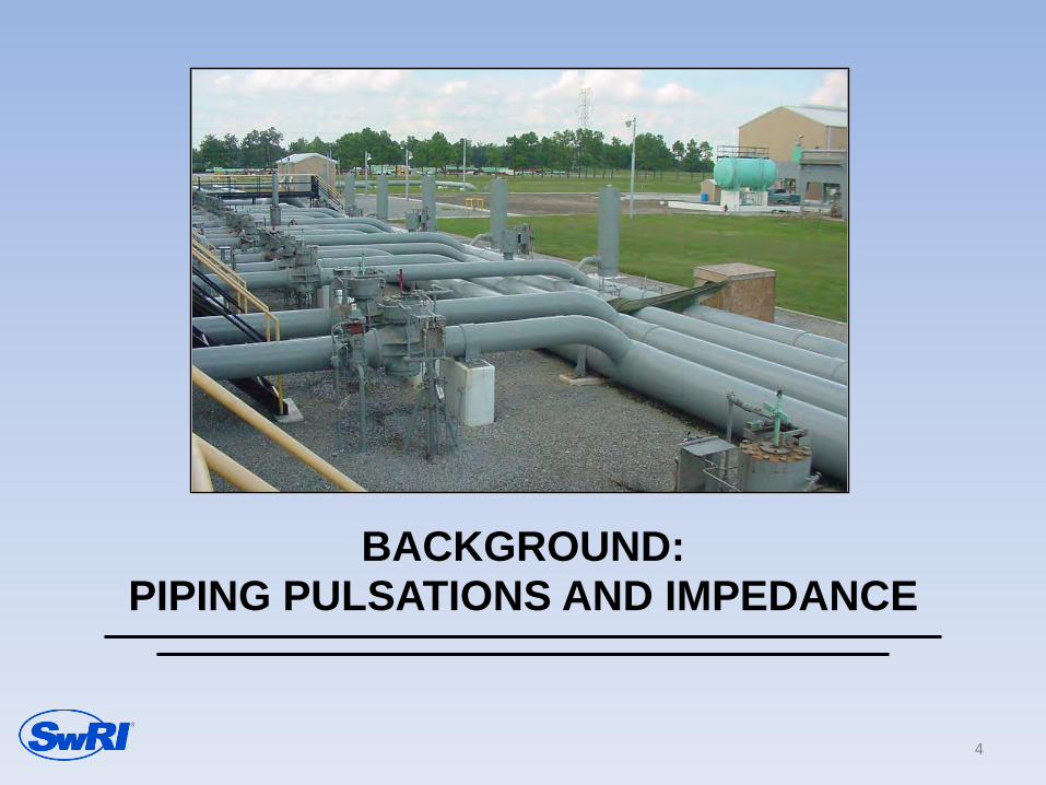
BACKGROUND: PIPING PULSATIONS AND IMPEDANCE
4

Pulsations: What are They?
• A traveling compression wave in a fluid • Fluid particles (molecules) force interaction • Waves are composed of two components: Pressure and Velocity • Waves move at the speed of sound. (Flow does not.)
Speed of sound, c, is function of fluid bulk modulus of fluid, B.
c2 = 𝑩𝝆
Link to animation webpage:
http://www.isvr.soton.ac.uk/SPCG/Tutorial/Tutorial/Tutorial_files/Web-basics-nature.htm
5

Half-wave Acoustic Response Frequency
Closed-closed configuration
Open-open configuration
Pressure minimum
at midpoint Pressure maximum
at midpoint
L2cnf =
f = Response frequency (Hz) c = Velocity of sound (ft/sec) L = Acoustic length of pipe span (ft) n = 1,2,3,…
6
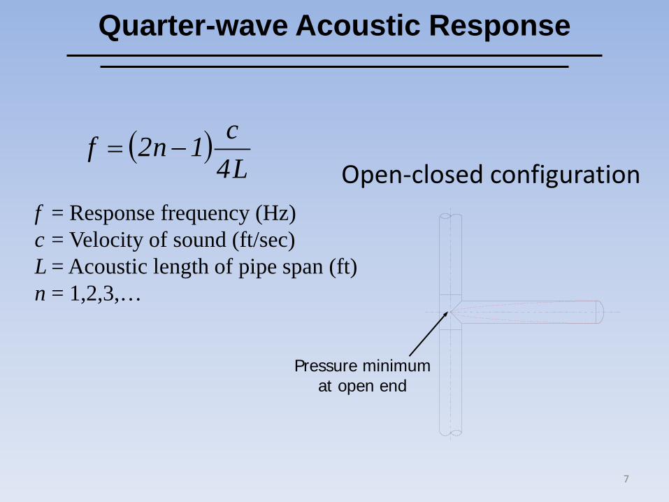
Quarter-wave Acoustic Response
Open-closed configuration
Pressure minimum at open end
f = Response frequency (Hz) c = Velocity of sound (ft/sec) L = Acoustic length of pipe span (ft) n = 1,2,3,…
( )L4c1n2f −=
7
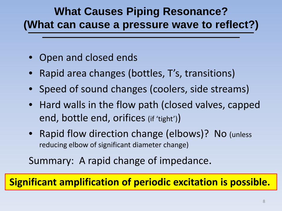
What Causes Piping Resonance? (What can cause a pressure wave to reflect?)
• Open and closed ends • Rapid area changes (bottles, T’s, transitions) • Speed of sound changes (coolers, side streams) • Hard walls in the flow path (closed valves, capped
end, bottle end, orifices (if ‘tight’)) • Rapid flow direction change (elbows)? No (unless
reducing elbow of significant diameter change)
Summary: A rapid change of impedance.
Significant amplification of periodic excitation is possible.
8
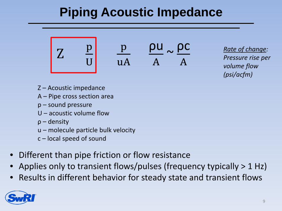
Piping Acoustic Impedance
Z = pU
= puA
= ρuA
~ ρcA
Z – Acoustic impedance A – Pipe cross section area p – sound pressure U – acoustic volume flow ρ – density u – molecule particle bulk velocity c – local speed of sound
• Different than pipe friction or flow resistance • Applies only to transient flows/pulses (frequency typically > 1 Hz) • Results in different behavior for steady state and transient flows
Rate of change: Pressure rise per volume flow (psi/acfm)
9
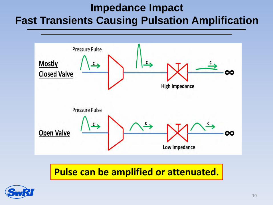
Impedance Impact Fast Transients Causing Pulsation Amplification
Pulse can be amplified or attenuated.
10

Discharge Pressure (Pd)
Volume Flow (V)
Ps Pd
Surge Line
Constant Suction Pressure Lines
Ps1
Ps2
Ps3
Low Impedance p ~ Z∙V
Valve Open
Surge
Compressor Map with Impedance Line Fast Transients Causing Surge
11

Pulsation Decay
0 5 10 15 20 25 30 Distance - Miles
Pres
sure
Dist
urba
nce
- psi
16
14
12
10
8
6
4
2
0
Decay of a 33Hz pulsation in a pipeline. Pulsation amplitude at inlet was 1% inlet pressure of 1500psi. [Kurz et al., 2003]
Pulsations can propagate over long distances 12
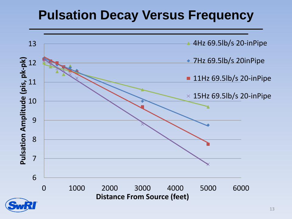
Pulsation Decay Versus Frequency
6
7
8
9
10
11
12
13
0 1000 2000 3000 4000 5000 6000
Puls
atio
n Am
plitu
de (p
is, p
k-pk
)
Distance From Source (feet)
4Hz 69.5lb/s 20-inPipe
7Hz 69.5lb/s 20inPipe
11Hz 69.5lb/s 20-inPipe
15Hz 69.5lb/s 20-inPipe
13

Centrifugal Compressor Map and Surge
-6
-4-2
0
24
6
810
12
0 1 2 3 4 5 6 7 8 9
Time [s]
CC
In
let
Flo
w [
m/s
]
Compressor Map
1
1.2
1.4
1.6
1.8
2
2.2
2.4
0.1 0.2 0.3 0.4 0.5 0.6 0.7 0.8 0.9
Flow*10 (kg/s)
Pres
sure
Rat
io (P
2/P1
)
8000 RPM
14300 RPM
10000 RPM
12000 RPM
Flow pulsations can cause periodic surge in centrifugal compressor
Surge
Brun et al. 2010
Surge
14

In Summary • Any flow unsteadiness or excitation in a piping system can be amplified by either
piping resonance or impedance decreasing compressor surge margin. • Periodic flow excitation (pulsations) can originate from vortex shedding, blade
passing and blade vane interactions, external pulsations, unstable flow control, check valve or relief valve chatter, diffuser rotating stall, and other process and aerodynamic flow instabilities.
• Low frequency pulsations require long distances to dampen out which is a consideration in mixed centrifugal and reciprocating compressor pipelines.
• Large discharge piping volumes with low impedances usually result in damping of pulsations, whereas high impedance systems (small piping volumes) can result in pulsation amplification. While it is desirable to limit the downstream volume between the compressor discharge and the check valve to reduce the potential for transient surge events during shutdowns, a small discharge volume can result in a high discharge piping impedance which can amplify pressure pulsations passing through the compressor.
A careful acoustic and impedance design review of a compressor station design should be performed to avoid impacting the
operating range of the machine and to properly balance these needs against the surge control system design requirements. 15

GMRC Surge Testing Project
Objective: • Determine whether pulsations from reciprocating compressors (RC),
vortex shedding or other sources can cause surge in centrifugal compressors (CC) when operating at low surge margin.
• Develop understanding of the physical process that causes pulsation induced CC surge.
• Determine the amplitude and frequency of pulsations required to cause CC surge. --- Then develop simple physical relationship or rules for pulsation induced surge avoidance (if ‘simple’ relationship is found).
• Determine impact of pulsations on performance. • Evaluate the impact and interaction of acoustic pipe resonances on
pulsation induced CC surge. • Evaluate the impact and interaction of pipe impedance on pulsation
induced CC surge. • Validate Compressor Dynamic Theory (Sparks et al., 1983) predictions for
pulsation amplification in centrifugal compressors.
16
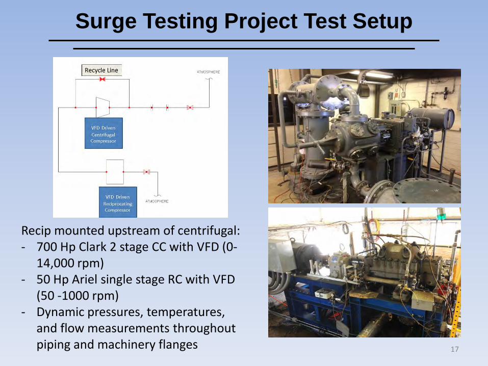
Surge Testing Project Test Setup
Recip mounted upstream of centrifugal: - 700 Hp Clark 2 stage CC with VFD (0-
14,000 rpm) - 50 Hp Ariel single stage RC with VFD
(50 -1000 rpm) - Dynamic pressures, temperatures,
and flow measurements throughout piping and machinery flanges 17

Surge Testing Project Test Approach
1. Operate CC at 8000 rpm with recycle valve wide open 2. Apply 300 rpm pulsation from recip to system 3. Close recycle valve (reduce flow) until surge is identified. 4. Back-off 2% SM% and sweep RC from 300 rpm to 1000 rpm. 5. Repeat step 4 with 4% and 6% surge margin. 6. Repeat steps 1 through 5 at 12,000 rpm
18
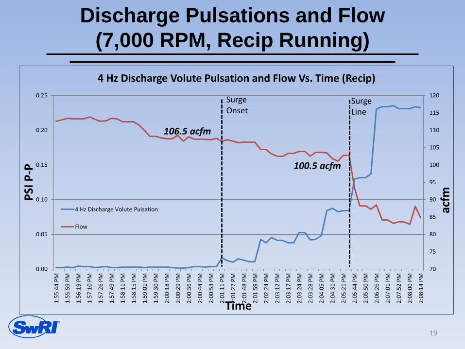
Discharge Pulsations and Flow (7,000 RPM, Recip Running)
19
70
75
80
85
90
95
100
105
110
115
120
0.00
0.05
0.10
0.15
0.20
0.25
1:55
:44
PM
1:55
:59
PM
1:56
:19
PM
1:57
:10
PM
1:57
:26
PM
1:57
:49
PM
1:58
:11
PM
1:58
:15
PM
1:59
:01
PM
1:59
:30
PM
2:00
:18
PM
2:00
:29
PM
2:00
:36
PM
2:00
:44
PM
2:00
:53
PM
2:01
:11
PM
2:01
:27
PM
2:01
:48
PM
2:01
:59
PM
2:02
:24
PM
2:03
:12
PM
2:03
:17
PM
2:03
:24
PM
2:03
:28
PM
2:04
:05
PM
2:04
:31
PM
2:05
:21
PM
2:05
:44
PM
2:05
:50
PM
2:06
:26
PM
2:07
:01
PM
2:07
:52
PM
2:08
:00
PM
2:08
:14
PM
acfm
PSI P
-P
Time
4 Hz Discharge Volute Pulsation and Flow Vs. Time (Recip)
4 Hz Discharge Volute Pulsation
Flow
Surge Onset
Surge Line
100.5 acfm
106.5 acfm
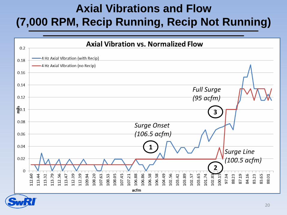
Axial Vibrations and Flow (7,000 RPM, Recip Running, Recip Not Running)
20
1
2
3
Surge Onset (106.5 acfm)
Surge Line (100.5 acfm)
Full Surge (95 acfm)
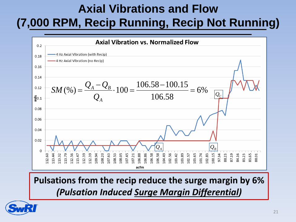
Pulsations from the recip reduce the surge margin by 6% (Pulsation Induced Surge Margin Differential)
Axial Vibrations and Flow (7,000 RPM, Recip Running, Recip Not Running)
21
AQ BQ
CQ%658.106
15.10058.106100(%) =−
=⋅−
=A
BA
QQQSM

%600332.
00312.00332.100(%) =−
=⋅Φ
Φ−Φ=
A
BASM
0
0.02
0.04
0.06
0.08
0.1
0.12
0.14
0.16
0.18
0.20.
0035
00.
0035
30.
0035
30.
0035
40.
0035
00.
0035
30.
0035
00.
0035
00.
0034
20.
0033
70.
0033
50.
0033
80.
0033
60.
0033
40.
0033
40.
0033
30.
0033
20.
0033
20.
0033
20.
0032
50.
0031
90.
0032
20.
0032
30.
0031
90.
0032
20.
0031
70.
0032
00.
0031
20.
0030
30.
0027
50.
0027
10.
0026
20.
0025
90.
0026
00.
0027
4
mils
Flow Coefficient
Axial Vibration vs. Flow Coefficient 4 Hz Axial Vibration (with Recip)
4 Hz Axial Vibration (no Recip)
AΦ BΦ
CΦ
Axial Vibrations and Flow (7,000 RPM, Recip Running, Recip Not Running)
22
Surge Margin Differential

1.04
1.06
1.08
1.1
1.12
1.14
1.16
1.18
1.2
1.22
70 100 130 160 190 220 250 280
Pres
sure
Rat
io
7000 RPM6 acfm
44 acfm
0.058 psi
Operating Map Ellipse: Pulsations and Flow Fluctuations
(7,000 RPM, Recip Running)
23
Operating Map Ellipse (zoom in on next slide)

Operating Map Ellipse: Surge Margin Differential and
Area Across Surge Line
24
25
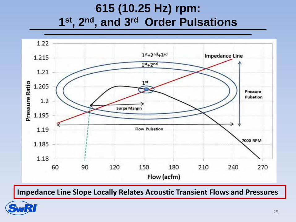
615 (10.25 Hz) rpm: 1st, 2nd, and 3rd Order Pulsations
Impedance Line Slope Locally Relates Acoustic Transient Flows and Pressures

Effect of Pressure and Flow Fluctuations on Surge (7,000 RPM, Recip Running)
26
Recip Speed (RPM) 405 (6.75 Hz)
480 (8 Hz)
615 (10.25 Hz)
Excitation Pulsations (psi pk-pk) [Pressure ratio fluctuations]
0.11 [0.0091]
0.13 [0.0108]
0.38 [0.0315]
Flow fluctuations (p-p acfm) [normalized]
90 [0.0028]
110 [0.0034]
250 [0.0078]
Flow at Surge (acfm) 102.5 121.0 150.8
Pressure Ratio at Surge 1.201 1.204 1.204
Surge Margin Differential % 7.9 24.3 41.2
% Area Across Surge Line 31 29 31
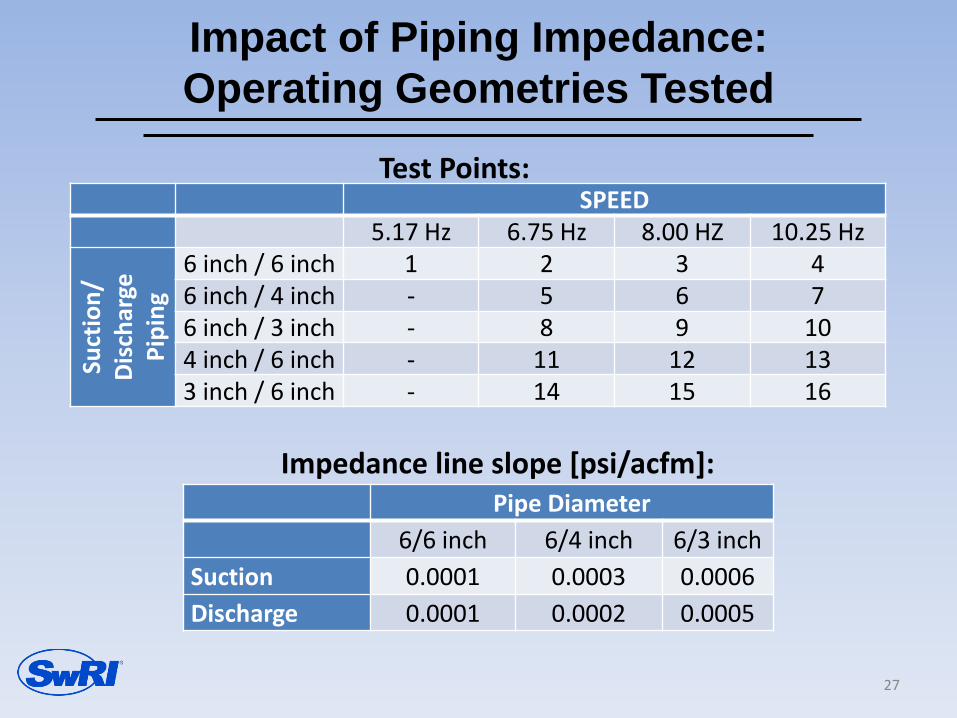
Impact of Piping Impedance: Operating Geometries Tested
SPEED 5.17 Hz 6.75 Hz 8.00 HZ 10.25 Hz
Suct
ion/
Di
scha
rge
Pipi
ng
6 inch / 6 inch 1 2 3 4 6 inch / 4 inch - 5 6 7 6 inch / 3 inch - 8 9 10 4 inch / 6 inch - 11 12 13 3 inch / 6 inch - 14 15 16
Pipe Diameter 6/6 inch 6/4 inch 6/3 inch Suction 0.0001 0.0003 0.0006 Discharge 0.0001 0.0002 0.0005
Impedance line slope [psi/acfm]:
Test Points:
27

Pulsation Amplification vs. Discharge Piping Impedance Slope
28
0.5
0.6
0.7
0.8
0.9
1
1.1
1.2
1.3
1.4
1.5
0 0.0001 0.0002 0.0003 0.0004 0.0005 0.0006
Puls
atio
n A
mpl
ifica
tion
Discharge Piping Impedance Slope [psi/acfm]
6/6
6/4
6/3

Impact of Piping Impedance General Trends
29
Increasing (“Steeper”)
Impedance Slope Decreasing (“Flatter”)
Impedance Slope
Suction Piping
↓↓↓ Surge Margin Differential
↑↑↑Surge Margin Differential
↑ Pulse Amplification ↓ Pulse Amplification
Discharge Piping
↓↓ Surge Margin Differential
↑↑ Surge Margin Differential
↑↑↑ Pulse Amplification ↓↓↓ Pulse Amplification
Consistent with Compressor Dynamic Response Theory
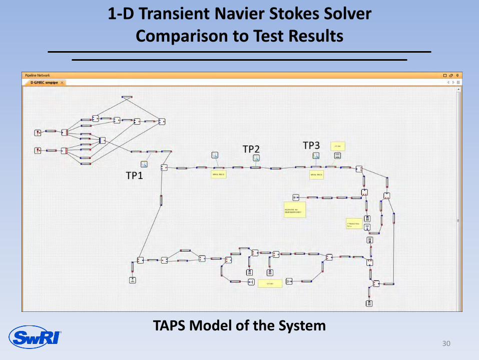
TAPS Model of the System
1-D Transient Navier Stokes Solver Comparison to Test Results
30
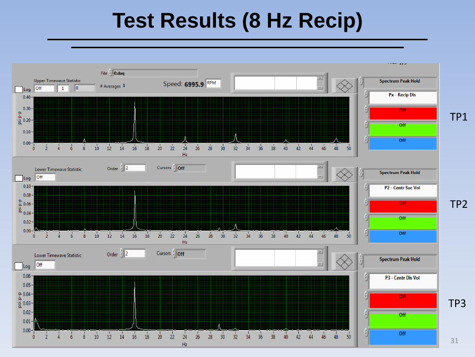
Test Results (8 Hz Recip)
TP1
TP2
TP3
31
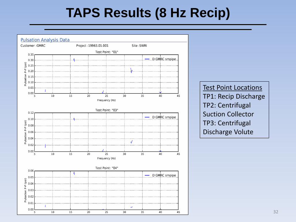
TAPS Results (8 Hz Recip)
Test Point Locations TP1: Recip Discharge TP2: Centrifugal Suction Collector TP3: Centrifugal Discharge Volute
32

DEVELOPMENT OF BASIC ENGINEERING GUIDELINE
33
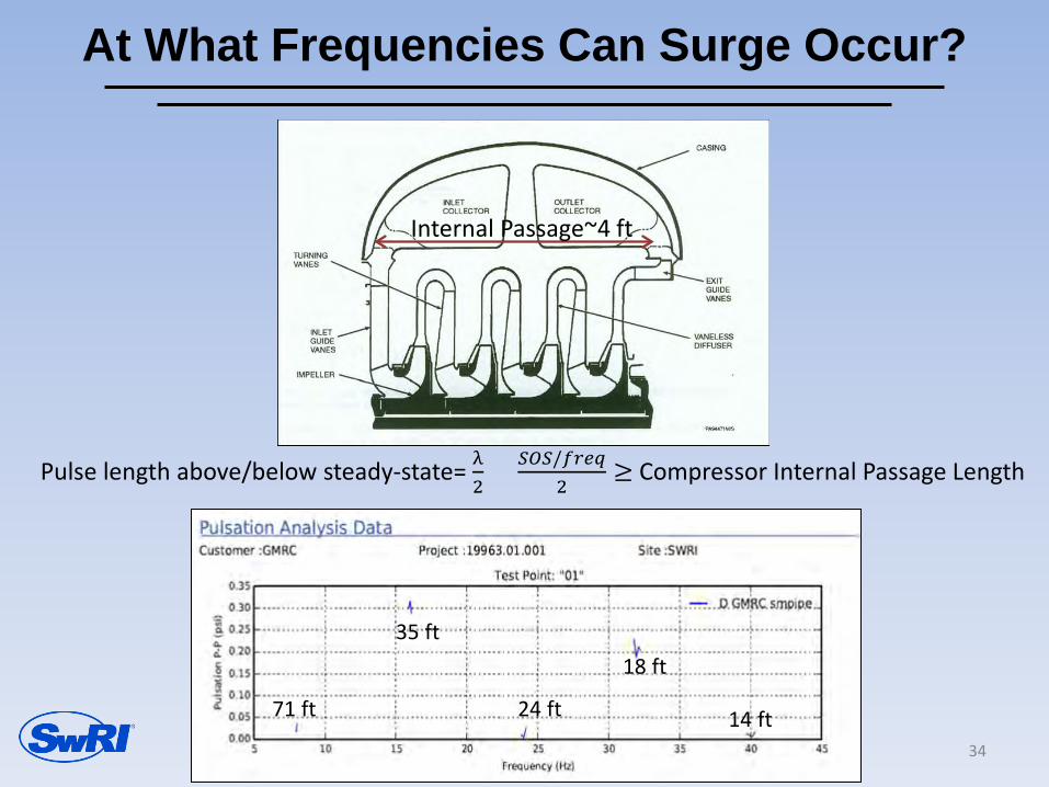
At What Frequencies Can Surge Occur?
Pulse length above/below steady-state= λ2
= 𝑆𝑆𝑆/𝑓𝑓𝑓𝑓2
≥ Compressor Internal Passage Length
71 ft
35 ft
24 ft
18 ft
14 ft
Internal Passage~4 ft
34
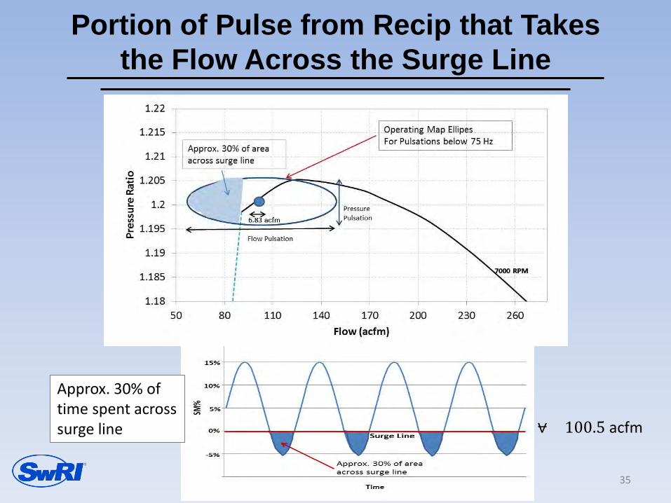
⩝= 100.5 acfm
Portion of Pulse from Recip that Takes the Flow Across the Surge Line
35
Approx. 30% of time spent across surge line
Conclusions
• External pulsations applied to the suction or discharge flange of a centrifugal compressor reduce its surge margin significantly.
• The geometry of the piping system immediately upstream and downstream of a centrifugal compressor can have significant impact on the surge margin reduction (surge margin differential).
• The reduction of surge margin due to external pulsations is a function of the pulsation amplitudes and frequencies at the compressor suction and discharge flange. High suction flange amplitudes at low frequencies significantly increase the risk of surge. Surge margin reductions (differentials) over 40% were observed during testing.
• Utilizing the transient operating map ellipse of the centrifugal compressor to identify whether induced pulsations can result in the operating point temporarily crossing the surge line is a useful tool to identify the potential onset of surge. From the operating map ellipse surge margin differential can be calculated for various orders of pulsations.
36

Conclusions (cont’d)
• If the upstream piping system impedance curve is flat, pressure pulses are converted to high volume flow pulses which increase the centrifugal compressor pulsation induced surge margin differential. On the other hand, steep piping impedance curves of the downstream piping reduce the surge margin differentials.
• Surge was consistently identified when approximately 30% of the area of the operating map ellipse had crossed the surge lines for all suction/ discharge pulsation frequencies orders under 75 Hz.
• A transient time domain 1-D Navier-Stokes pipe network analysis model was able to accurately predict suction/ discharge pulsations into a centrifugal compressor and thus, its operating map ellipse. Using the basic design rule ‘30% of the operating map area across the surge line for all pulsations below 75 Hz’, these pressure/ flow pulsation amplitude predictions can be related to surge margin differential.
37

Thanks! Any Questions?
Ms. Sarah Simons Contact info: Southwest Research Institute Tel: 210 522 2418 [email protected]
Eugene ‘Buddy’ Broerman Contact info: Southwest Research Institute Tel: 210 522 2555 [email protected]
38

Thermal Piping Flexibility
1
by Benjamin A. White, P.E.
Manager, R&D Fluid Machinery Systems
Southwest Research Institute
San Antonio, Texas Presented at the 2016
Gas/Electric Partnership Houston, Texas February 2, 2016

Thermal Analyses
• Most compressor units have elevated discharge gas temperatures.
• This causes thermal expansion of the piping. • As a result, loads and stresses are generated.
• Static stresses (not dynamic).
2
Also Called: Piping Stress Analysis
Thermal Flexibility Analysis
Thermal Analysis
3
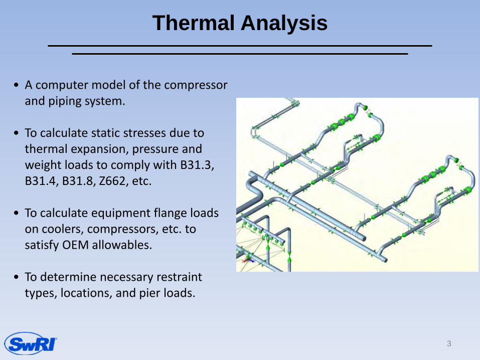
• A computer model of the compressor and piping system.
• To calculate static stresses due to thermal expansion, pressure and weight loads to comply with B31.3, B31.4, B31.8, Z662, etc.
• To calculate equipment flange loads on coolers, compressors, etc. to satisfy OEM allowables.
• To determine necessary restraint types, locations, and pier loads.
Thermal Analysis
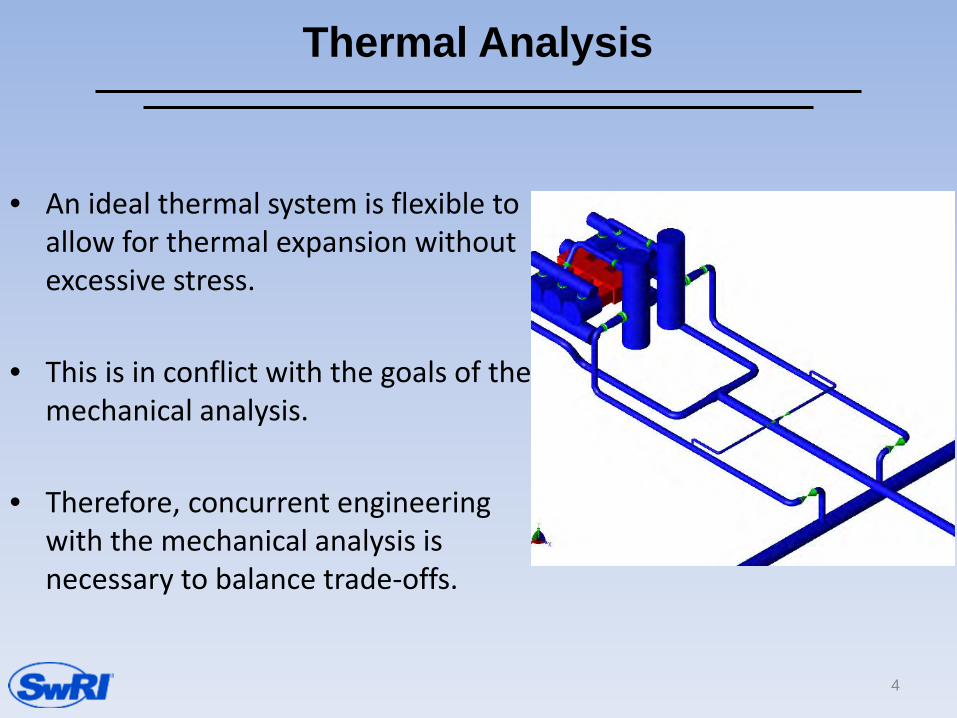
• An ideal thermal system is flexible to allow for thermal expansion without excessive stress.
• This is in conflict with the goals of the mechanical analysis.
• Therefore, concurrent engineering with the mechanical analysis is necessary to balance trade-offs.
4
When to Do an Analysis
• There is no absolute criteria. • Typically done when:
– Operating temperatures above 130 °F (54 °C) – Large diameter piping (12” and above) – Design not similar to past installations – There are critical equipment load allowables (cooler/compressors/etc.) – Critical applications (offshore, etc.) – When required by piping code
• B31.8 Section 833.7 says a formal flexibility analysis is not required if the system duplicates without significant change a system operating with a successful record or can be readily judged adequate by comparison with previously analyzed systems.
5

Thermal Analysis Basics
6
• Thermal expansion is a function of : • Pipe length • Temperature differential • Expansion coefficient (≅ 6.5e-6 in/in-deg for Carbon Steel) • Growth = a Expansion Coefficient * Length * ∆T • For a 100’ long pipe at 180 °F
• Growth = 6.3e-6 * (100*12) * (180-70) = 0.832”
• Stress is a function of : • Amount of thermal growth • Pipe size and layout • Restraint Types and Locations • Allowable stress related to the design code, material, load case, etc.

Thermal Analysis Basics
7
Building The Model
8
• Commercial Software Package (Caesar II, AutoPIPE, etc.)
• Determine extent of model(s) • Whole System vs. Isolated Line • Skid Package Termination? • Multiple parties involved? • “Anchor” terminations?
Building The Model
9
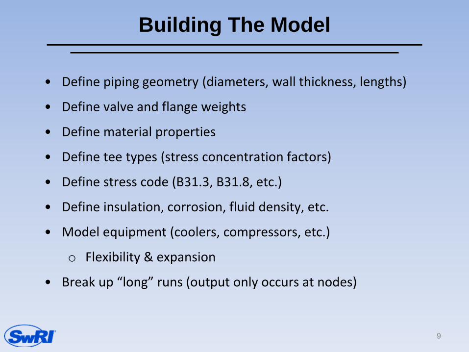
• Define piping geometry (diameters, wall thickness, lengths)
• Define valve and flange weights
• Define material properties
• Define tee types (stress concentration factors)
• Define stress code (B31.3, B31.8, etc.)
• Define insulation, corrosion, fluid density, etc.
• Model equipment (coolers, compressors, etc.)
o Flexibility & expansion
• Break up “long” runs (output only occurs at nodes)

Building The Model - Restraints
• Different restraints have different stiffness properties – Simple weight supports
– Guides, stops, spring cans and hangers
– Box clamps
– U-bolts
– Strap-type hold down clamps – best for vibration control
• Restraints are not rigid
• For accurate modeling predictions, it is essential to accurately estimate stiffness in all directions
• Piping restraints are initially selected based on dynamics (vibration control). Thermal considerations done later.
• Soil restraints <<<
10
Building the Model Temperature & Pressures
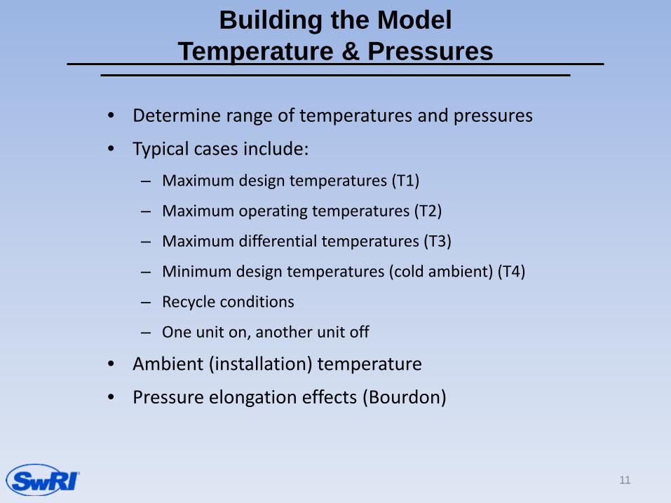
• Determine range of temperatures and pressures
• Typical cases include: – Maximum design temperatures (T1)
– Maximum operating temperatures (T2)
– Maximum differential temperatures (T3)
– Minimum design temperatures (cold ambient) (T4)
– Recycle conditions
– One unit on, another unit off
• Ambient (installation) temperature
• Pressure elongation effects (Bourdon)
11

Load Cases
12
• Operating Load Cases (Weight + Pressure + Temp.)
• Primarily for Nozzle and Restraint Loads
• Sustained Load Cases (Weight + Pressure)
• Expansion Load Cases (Temp. Only) – OPE-SUS “self-limiting
loads”
• Primarily for Pipe Stress
• Total Temperature (Displacement) Range Expansion Load Case <<<
• Occasional Loads (Wind, Seismic)
• Hot Sustained Load Case (restraint lift off)
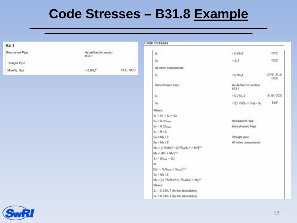
Code Stresses – B31.8 Example
13

Output to Review
14
• Software Calculates: Stresses, Displacements and Loads
• Animate Deflections and Modal Run for Error Check
• Stresses – Code Compliance
• Centrifugal Compressor Nozzle Loads – API 617, etc.
• Cooler Loads – API 661, etc.
• Clamp Loads – (high loads, lifting and displacement)
• Other Equipment or Vessel Loads
• Consider Displacements where Loads are High!
• Modal run for vibration characteristics

Typical Solutions
15
• Solution depends on the specifics of the problem
• Common solutions:
• Change restraint types, locations or quantity
• Re-route piping (add offset or expansion loop)
• Replace 45° degree elbows with 90° degree elbows
• Change tee type or use larger bore tee with reducer
• The following slides illustrate some of these ideas

High Stress at Tee – A Common Problem
16
The mainline moves
The branch line is restrained. - Try shifting clamp or changing type. Stress develops here (depending
on the SIF of the particular joint type). - Try a larger branch or tee type with lower SIF.
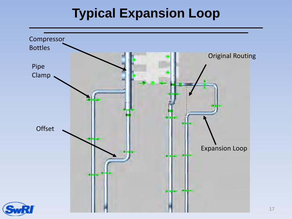
Typical Expansion Loop
17
Offset
Expansion Loop
Original Routing Pipe Clamp
Compressor Bottles

Thermal Piping Layout Near Compressor • Compressor Nozzle Loads
– Thermal, Weight & Pressure
– API 617 or NEMA SM23 (allowable multiplier)
– Individual and Combined Allowables • Special Supports Near Unit
– Axial Pipe Stop (Anchor) • Piping Offset to Absorb Thermal Expansion
– Horizontal or Vertical • Suction Flange Loads (resolving moments)
• Function of Pipe Diameter 18

BALANCING VIBRATION CONSIDERATIONS
• Consider Clamp Types… – Does it allow thermal expansion?
– Does it control vibration?
• Slotted Bolt Holes – Static vs. Dynamic loads
• Locations >> Which Side of an Elbow?
19
Centrifugal Compressor Nozzle Loads
20
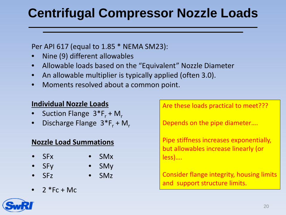
Per API 617 (equal to 1.85 * NEMA SM23): • Nine (9) different allowables • Allowable loads based on the “Equivalent” Nozzle Diameter • An allowable multiplier is typically applied (often 3.0). • Moments resolved about a common point.
Individual Nozzle Loads • Suction Flange 3*Fr + Mr • Discharge Flange 3*Fr + Mr
Nozzle Load Summations
• 2 *Fc + Mc
• SFx • SFy • SFz
• SMx • SMy • SMz
Are these loads practical to meet??? Depends on the pipe diameter…. Pipe stiffness increases exponentially, but allowables increase linearly (or less)…. Consider flange integrity, housing limits and support structure limits.
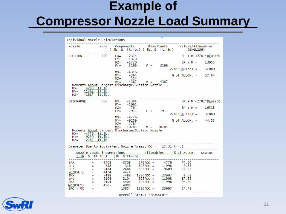
Example of Compressor Nozzle Load Summary
21

Thermal Piping Layout Near Cooler
• Cooler Nozzle Loads – Thermal, Weight & Pressure – API 661 (allowable multiplier) – Individual and Header Allowables
• Piping Offsets • Function of Pipe Diameter • Vibration Considerations
– Balance Vibration vs. Cooler Loads – Top vs. Bottom Inlet – Clamp Types and Locations
22

QUESTIONS?
23
Benjamin A. White, P.E. Contact info: Southwest Research Institute Tel: 210-522-2554 [email protected]