CENTRE FOR STOCHASTIC GEOMETRY AND ... -...
48
CENTRE FOR STOCHASTIC GEOMETRY AND ADVANCED BIOIMAGING www.csgb.dk RESEARCH REPORT 2010 Adrian Baddeley, Ege Rubak and Jesper Møller Score, pseudo-score and residual diagnostics for goodness-of-fit of spatial point process models No. 04, June 2010
Transcript of CENTRE FOR STOCHASTIC GEOMETRY AND ... -...

CENTRE FOR STOCHASTIC GEOMETRYAND ADVANCED BIOIMAGING
www.csgb.dk
RESEARCH REPORT
2010Adrian Baddeley, Ege Rubak and Jesper Møller
Score, pseudo-score and residual diagnostics forgoodness-of-fit of spatial point process models
No. 04, June 2010

Submitted to the Statistical Science
Score, pseudo-score andresidual diagnostics forgoodness-of-fit of spatial pointprocess modelsAdrian Baddeley, Ege Rubak and Jesper Møller
CSIRO and Aalborg University
Abstract.Wedevelop new tools for formal inference and informal modelvalidation in the analysis of spatial point pattern data. The score testis generalised to a ‘pseudo-score’ test derived from Besag’s pseudo-likelihood, and to a class of diagnostics based on point process resid-uals. The results lend theoretical support to the established practiceof using functional summary statistics such as Ripley’s K-function,when testing for complete spatial randomness; and they provide newtools such as the compensator of the K-function for testing other fit-ted models. The results also support localisation methods such as thescan statistic and smoothed residual plots. Software for computing thediagnostics is provided.
AMS 2000 subject classifications: Primary 62M30; secondary 62J20.Key words and phrases: compensator, functional summary statistics,modelvalidation, point process residuals, pseudo-likelihood.
CSIROMathematics, Informatics and Statistics, Private Bag 5, Wembley WA 6913,Australia. (e-mail: [email protected]). Department of Mathematical Sciences,Aalborg University, Fredrik Bajers Vej 7G, DK-9220 Aalborg Ø, Denmark (e-mail:[email protected]; [email protected]).
1

2 A. BADDELEY ET AL.
1. INTRODUCTION
This paper develops new tools for formal inference and informal model valid-ation in the analysis of spatial point pattern data. The score test statistic, basedon the point process likelihood, is generalised to a ‘pseudo-score’ test statis-tic derived from Besag’s pseudo-likelihood. The score and pseudo-score can beviewed as residuals, and further generalised to a class of residual diagnostics.
The likelihood score and the score test [73, 60], [21, pp 315 and 324] are usedfrequently in applied statistics to provide diagnostics for model selection andmodel validation [2, 18, 59, 15, 75]. In spatial statistics, the score test is usedmainly to support formal inference about covariate effects [13, 46, 74] assumingthe underlying point process is Poisson under both the null and alternative hy-potheses. Our approach extends this to a much wider class of point processes,making it possible (for example) to check for covariate effects or localised hot-spots in a clustered point pattern.
Figure 1 shows three example datasets studied in the paper. Our techniquesmake it possible to check separately for ‘inhomogeneity’ (spatial variation inabundance of points) and ‘interaction’ (localised dependence between points)in these data.
(a) (b) (c)
Fig 1: Point pattern datasets. (a) Japanese black pine seedlings and saplings in a10 × 10 metre quadrat [52, 53]. Reprinted by kind permission of Professors M.Numata and Y. Ogata. (b) Simulated realisation of inhomogeneous Strauss pro-cess showing strong inhibition and spatial trend [6, Fig. 4b]. (c) Simulated re-alisation of homogeneous Geyer saturation process showing moderately strongclustering without spatial trend [6, Fig. 4c].
Our approach also provides theoretical support for the established practice ofusing functional summary statistics such as Ripley’sK-function [62, 63] to studyclustering and inhibition between points. In one class of models, the score teststatistic is equivalent to the empiricalK-function, and the score test procedure isclosely related to the customary goodness-of-fit procedure based on comparingthe empirical K-function with its null expected value. Similar statements applyto the nearest neighbour distance distribution function G and the empty spacefunction F .
For computational efficiency, especially in large datasets, the point processlikelihood is often replaced by Besag’s [14] pseudo-likelihood. The resulting‘pseudo-score’ is a possible surrogate for the likelihood score. In one model,the pseudo-score test statistic is equivalent to a residual version of the empirical

GOODNESS-OF-FIT FOR SPATIAL POINT PROCESSES 3
K-function, yielding a new, efficient diagnostic for goodness-of-fit. However, ingeneral, the interpretation of the pseudo-score test statistic is conceptually morecomplicated than that of the likelihood score test statistic, and hence difficult toemploy as a diagnostic.
In classical settings the score test statistic is a weighted sum of residuals. Herethe pseudo-score test statistic is a weighted point process residual in the senseof [6, 3]. This suggests a simplification, in which the pseudo-score test statisticis replaced by another residual diagnostic that is easier to interpret and to com-pute.
0.00 0.02 0.04 0.06 0.08 0.10 0.12
0.00
0.01
0.02
0.03
0.04
K(r)CK(r)CSR
Fig 2: Empirical K-function (thick grey line) for the point pattern data in Fig-ure 1b, compensator of the K-function (solid black line) for a model of the cor-rect form, and expectedK-function for a homogeneous Poisson process (dashedline).
In special cases this diagnostic is a residual version of one of the classical func-tional summary statisticsK ,G or F obtained by subtracting a ‘compensator’ fromthe functional summary statistic. The compensator depends on the observeddata and on the fitted model. For example, if the fitted model is the homoge-neous Poisson process, then the compensator of G(r) is F (r), and the compen-sator of K(r) is πr2. This approach provides a new class of residual summarystatistics that can be used as informal diagnostics for goodness-of-fit, for a widerange of point process models, in close analogy with current practice. The di-agnostics apply under very general conditions, including the case of inhomo-geneous point process models, where exploratory methods are underdevelopedor inapplicable. For instance, the compensator of K(r) for an inhomogeneousnon-Poisson model is illustrated in Figure 2.
Section 2 introduces basic definitions and assumptions. Section 3 describesthe score test for a general point process model, and Section 4 develops the im-portant case of Poisson point process models. Section 5 gives examples and tech-nical tools for non-Poisson point process models. Section 6 develops the generaltheory for our diagnostic tools. Section 7 applies these tools to tests for first ordertrend and hotspots. Sections 8–11 develop diagnostics for interaction betweenpoints, based on pairwise distances, nearest neighbour distances and emptyspace distances respectively. The tools are demonstrated on data in Sections 12–

4 A. BADDELEY ET AL.
15. Further examples of diagnostics are given in Appendix A. Appendices B–Eprovide technical details.
2. ASSUMPTIONS
2.1 Fundamentals
A spatial point pattern dataset is a finite setx = {x1, . . . , xn} of points xi ∈ W ,where the number of points n(x) = n ≥ 0 is not fixed in advance, and thedomain of observationW ⊂ Rd is a fixed, known region of d-dimensional spacewith finite positive volume |W |. We take d = 2 but the results generalise easilyto all dimensions.
A point process model assumes that x is a realisation of a finite point processX in W without multiple points. We can equivalently view X as a random fi-nite subset of W . Much of the literature on spatial statistics assumes that X isthe restriction X = Y ∩ W of a stationary point process Y on the entire spaceR2. We do not assume this; there is no assumption of stationarity, and someof the models considered here are intrinsically confined to the domain W . Forfurther background material including measure theoretical details, see e.g. [50,Appendix B].
WriteX ∼ Poisson(W,ρ) ifX follows the Poisson process onW with intensityfunction ρ, where we assume ν =
∫W ρ(u) du is finite. Then n(X) is Poisson
distributed with mean ν, and conditional on n(X), the points in X are i.i.d.with density ρ(u)/ν.
Every point process model considered here is assumed to have a probabilitydensity with respect to Poisson(W, 1), the unit rate Poisson process, under oneof the following scenarios.
2.2 Unconditional case
In the unconditional casewe assumeX has a density f with respect toPoisson(W, 1).Then the density is characterised by the property
(1) E[h(X)] = E[h(Y )f(Y )]
for all non-negative measurable functionals h, where Y ∼ Poisson(W, 1). In par-ticular the density of Poisson(W,ρ) is
(2) f(x) = exp
(∫
W(1− ρ(u)) du
)∏
i
ρ(xi).
We assume that f is hereditary, i.e. f(x) > 0 implies f(y) > 0 for all finitey ⊂ x ⊂ W .
2.3 Conditional case
In the conditional case, we assume X = Y ∩ W where Y is a point process.Thus X may depend on unobserved points of Y lying outside W . The densityof X may be unknown or intractable. Under suitable conditions (explained inSection 5.4) modelling and inference can be based on the conditional distributionof X◦ = X ∩W ◦ given X+ = X ∩W+ = x+, where W+ ⊂ W is a subregion,typically a region near the boundary ofW , and only the points inW ◦ = W \W+
are treated as random. We assume that the conditional distribution of X◦ =

GOODNESS-OF-FIT FOR SPATIAL POINT PROCESSES 5
X ∩W ◦ given X+ = X ∩W+ = x+ has an hereditary density f(x◦ | x+) withrespect to Poisson(W ◦, 1).
For ease of exposition, we focus mainly on the unconditional case, with occa-sional comments on the conditional case. For Poisson point process models, wealways takeW = W ◦ so that the two cases agree.
3. SCORE TEST FOR POINT PROCESSES
In principle, any technique for likelihood-based inference is applicable to pointprocess likelihoods. In practice, many likelihood-based computations requireextensive Monte Carlo simulation [30, 50, 49]. To minimise such difficulties,when assessing the goodness-of-fit of a fitted point processmodel, it is natural tochoose the score test which only requires computations for the null hypothesis[73, 60].
Consider any parametric family of point process models for X with densityfθ indexed by a k-dimensional vector parameter θ ∈ Θ ⊆ Rk. For a simple nullhypothesisH0 : θ = θ0 where θ0 ∈ Θ is fixed, the score test against any alterna-tive H1 : θ ∈ Θ1, where Θ1 ⊆ Θ \ {θ0}, is based on the score test statistic [21, p.315]
(3) T 2 = U(θ0)TI(θ0)
−1U(θ0).
Here U(θ) = ∂∂θ log fθ(x) and I(θ) = Eθ
[U(θ)U(θ)T
]are the score function and
Fisher information respectively, and the expectation is with respect to fθ. Hereand throughout, we assume that the order of integration and differentation withrespect to θ can be interchanged. Under suitable conditions, the null distributionof T 2 is χ2 with k degrees of freedom. In the case k = 1 it may be informative toevaluate the signed square root
(4) T = U(θ0)/√
I(θ0)
which is asymptotically standard normally distributed under the same condi-tions.
For a composite null hypothesisH0 : θ ∈ Θ0 whereΘ0 ⊂ Θ is anm-dimensionalsubmanifold with 0 < m < k, the score test statistic is defined in [21, p. 324].However, we shall not use this version of the score test, as it assumes differ-entiability of the likelihood with respect to nuisance parameters, which is notnecessarily applicable here (as exemplified in Section 4.2).
In the sequel we often consider models of the form
(5) f(α,β)(x) = c(α, β)hα(x) exp(βS(x))
where the parameter β and the statistic S(x) are one dimensional, and the nullhypothesis is H0 : β = 0. For fixed α, this is a linear exponential family and (4)becomes
T (α) =(S(x)− E(α,0)[S(x)]
)/√
Var(α,0)[S(x)].
In practice, when α is unknown, we replace α by its MLE under H0 so that,with a slight abuse of notation, the signed square root of the score test statisticis approximated by
(6) T = T (α) =(S(x)− E(α,0)[S(x)]
)/√
Var(α,0)[S(x)].

6 A. BADDELEY ET AL.
Under suitable conditions, T in (6) is asymptotically equivalent to T in (4), andso a standard Normal approximation may still apply.
4. SCORE TEST FOR POISSON PROCESSES
Application of the score test to Poisson point process models appears to origi-nate with Cox [20]. Consider a parametric family of Poisson processes,Poisson(W,ρθ),where the intensity function is indexed by θ ∈ Θ. The score test statistic is (3)where
U(θ) =∑
i
κθ(xi)−∫
Wκθ(u)ρθ(u) du
I(θ) =
∫
Wκθ(u) κθ(u)
Tρθ(u) du
with κθ(u) =∂∂θ log ρθ(u). Asymptotic results are given in [44, 61].
4.1 Log-linear alternative
The score test is commonly used in spatial epidemiology to assess whetherdisease incidence depends on environmental exposure. As a particular case of(5), suppose the Poisson model has a log-linear intensity function
(7) ρ(α,β)(u) = exp(α+ βZ(u))
whereZ(u), u ∈ W is a known, real-valued and non-constant covariate function,and α and β are real parameters. Cox [20] noted that the uniformly most pow-erful test of H0 : β = 0 (the homogeneous Poisson process) against H1 : β > 0 isbased on the statistic
(8) S(x) =∑
i
Z(xi).
Recall that, for a point processX on W with intensity function ρ,
(9) E
∑
xi∈Xh(xi)
=
∫
Wh(u)ρ(u) du
for any Borel function h such that the integral on the right hand side exists, andfor Poisson(W,ρ),
(10) Var
∑
xi∈Xh(xi)
=
∫
Wh(u)2ρ(u) du
for any Borel function h such that the integral on the right hand side exists [23,p. 188]. Hence the standardised version of (8) is
(11) T =
(S(x)− κ
∫
WZ(u) du
)/√κ
∫
WZ(u)2 du
where κ = n/|W | is the MLE of the intensity κ = exp(α) under the null hypoth-esis. This is a direct application of the approximation (6) of the signed squareroot of the score test statistic.

GOODNESS-OF-FIT FOR SPATIAL POINT PROCESSES 7
Berman [13] proposed several tests and diagnostics for spatial associationbetween a point process X and a covariate function Z(u). Berman’s Z1 test isequivalent to the Cox score test described above. Waller et al. [74] and Lawson[46] proposed tests for the dependence of disease incidence on environmentalexposure, based on data giving point locations of disease cases. These are alsoapplications of the score test. Berman conditioned on the number of points whenmaking inference. This is in accordance with the observation that the statisticn(x) is S-ancillary for β, while S(x) is S-sufficient for β.
4.2 Threshold alternative and nuisance parameters
Consider the Poisson process with an intensity function of ‘threshold’ form,
ρz,κ,φ(u) =
{κ exp(φ) if Z(u) ≤ zκ if Z(u) > z
where z is the threshold level. If z is fixed, this model is a special case of (7) withZ(u) replaced by I{Z(u) ≤ z}, and so (8) is replaced by
S(x) = S(x, z) =∑
i
I{Z(xi) ≤ z}
where I{·} denotes the indicator function. By (11) the (approximate) score test ofH0 : φ = 0 against H1 : φ 6= 0 is based on
T = T (z) = (S(x, z) − κA(z)) /√
κA(z)
where A(z) = |{u ∈ W : Z(u) ≤ z}| is the area of the corresponding level set ofZ .
If z is not fixed, then it plays the role of a nuisance parameter in the score test:the value of z affects inference about the canonical parameter φ, which is theparameter of primary interest in the score test. Note that the likelihood is notdifferentiable with respect to z.
In most applications of the score test, a nuisance parameter would be replacedby its MLE under the null hypothesis. However in this context, z is not identi-fiable under the null hypothesis. Several approaches to this problem have beenproposed [17, 24, 25, 32, 67]. They include replacing z by its MLE under the alter-native [17], maximising T (z) or |T (z)| over z [24, 25], and finding the maximump-value of T (z) or |T (z)| over a confidence region for z under the alternative[67].
These approaches appear to be inapplicable to the current context. While thenull distribution of T (z) is asymptoticallyN(0, 1) for each fixed z as κ → ∞, thisconvergence is not uniform in z. The null distribution of S(x, z) is Poisson withparameter κA(z); sample paths of T (z) will be governed by Poisson behaviourwhere A(z) is small.
In this paper, our approach is simply to plot the score test statistic as a functionof the nuisance parameter. This turns the score test into a graphical exploratorytool, following the approach adopted in many other areas [2, 18, 59, 15, 75]. Asecond style of plot based on S(x, z) − κA(z) against z may be more appro-priate visually. Such a plot is the lurking variable plot of [6]. Berman [13] alsoproposed a plot of S(x, z) against z, together with a plot of κA(z) against z, as

8 A. BADDELEY ET AL.
a diagnostic for dependence on Z . This is related to the Kolmogorov-Smirnovtest since, under H0, the values Yi = Z(xi) are i.i.d. with distribution functionP(Y ≤ y) = A(z)/|W |.4.3 Hot spot alternative
Consider the Poisson process with intensity
(12) ρκ,φ,v(u) = κ exp(φk(u− v))
where k is a kernel (a probability density onR2), κ > 0 and φ are real parameters,and v ∈ R2 is a nuisance parameter. This process has a ‘hot spot’ of elevatedintensity in the vicinity of the location v. By (11) and (9)–(10) the score test ofH0 : φ = 0 against H1 : φ 6= 0 is based on
T = T (v) = (S(x, v) − κM1(v))/√
κM2(v)
whereS(x, v) =
∑
i
k(xi − v)
is the usual nonparametric kernel estimate of point process intensity [27] evalu-ated at v without edge correction, and
Mi(v) =
∫
Wk(u− v)i du, i = 1, 2.
The numerator S(x, v)−κM1(v) is the smoothed residual field [6] of the null model.In the special case where k(u) ∝ I{‖u‖ ≤ h} is the uniform density on a disc ofradius h, the maximum maxv T (v) is closely related to the scan statistic [1, 43].
5. NON-POISSON MODELS
The remainder of the paper deals with the case where the alternative (andperhaps also the null) is not a Poisson process. Key examples are stated in Sec-tion 5.1. Non-Poisson models require additional tools including the conditionalintensity (Section 5.2) and pseudo-likelihood (Section 5.3).
5.1 Point process models with interaction
We shall frequently consider densities of the form
(13) f(x) = c
[∏
i
λ(xi)
]exp (φV (x))
where c is a normalising constant, the first order term λ is a non-negative func-tion, φ is a real interaction parameter, and V (x) is a real non-additive functionwhich specifies the interaction between the points. We refer to V as the interac-tion potential. In general, apart from the Poisson density (2) corresponding tothe case φ = 0, the normalising constant is not expressible in closed form.
Often the definition of V can be extended to all finite point patterns inR2 so asto be invariant under rigid motions (translations and rotations). Then the modelfor X is said to be homogeneous if λ is constant on W , and inhomogeneousotherwise.

GOODNESS-OF-FIT FOR SPATIAL POINT PROCESSES 9
Letd(u,x) = min
j‖u− xj‖
denote the distance from a location u to its nearest neighbour in the point con-figuration x. For n(x) = n ≥ 1 and i = 1, . . . , n, define
x−i = x \ {xi}.
In many places in this paper we consider the following three motion-invariantinteraction potentials V (x) = V (x, r) depending on a parameter r > 0 whichspecifies the range of interaction. The Strauss process [71] has interaction poten-tial
(14) VS(x, r) =∑
i<j
I{‖xi − xj‖ ≤ r}
the number of r-close pairs of points in x; the Geyer saturation model [30] withsaturation threshold 1 has interaction potential
(15) VG(x, r) =∑
i
I{d(xi,x−i) ≤ r}
the number of points in x whose nearest neighbour is closer than r units; andthe Widom-Rowlinson penetrable sphere model [76] or area-interaction process[11] has interaction potential
(16) VA(x, r) = −|W ∩⋃
i
B(xi, r)|
the negative area of W intersected with the union of balls B(xi, r) of radius rcentred at the points of x. Each of these densities favours spatial clustering (pos-itive association) when φ > 0 and spatial inhibition (negative association) whenφ < 0. The Geyer and area-interaction models are well-defined point processesfor any value of φ [11, 30], but the Strauss density is integrable only when φ ≤ 0[42].
5.2 Conditional intensity
Consider a parametric model for a point process X in R2, with parameterθ ∈ Θ. Papangelou [58] defined the conditional intensity of X as a non-negativestochastic process λθ(u,X) indexed by locations u ∈ R2 and characterised bythe property that
(17) Eθ
∑
xi∈Xh(xi,X \ {xi})
= Eθ
[∫
R2
h(u,X)λθ(u,X) du
]
for all measurable functions h such that the left or right hand side exists. Equa-tion (17) is known as theGeorgii-Nguyen-Zessin (GNZ) formula [29, 40, 41, 51]; seealso Section 6.4.1 in [50]. Adapting a term from stochastic process theory, we willcall the random integral on the right side of (17) the (Papangelou) compensator ofthe random sum on the left side.

10 A. BADDELEY ET AL.
Consider a finite point processX inW . In the unconditional case (Section 2.2)we assumeX has density fθ(x)which is hereditary for all θ ∈ Θ. Wemay simplydefine
(18) λθ(u,x) = fθ(x ∪ {u})/fθ(x)for all locations u ∈ W and point configurations x ⊂ W such that u 6∈ x. Herewe take 0/0 = 0. For xi ∈ x we set λθ(xi,x) = λθ(xi,x−i), and for u 6∈ W we setλθ(u,x) = 0. Then it may be verified directly from (1) that (17) holds, so that (18)is the Papangelou conditional intensity ofX . Note that the normalising constantof fθ cancels in (18). For a Poisson process, it follows from (2) and (18) that theconditional intensity is equivalent to the intensity function of the process.
In the conditional case (Section 2.3) we assume that the conditional distribu-tion of X◦ = X ∩ W ◦ given X+ = X ∩ W+ = x+ has an hereditary densityfθ(x
◦ | x+) with respect to Poisson(W ◦, 1), for all θ ∈ Θ. Then define
(19) λθ(u,x◦ | x+) = fθ(x
◦ ∪ {u} | x+)/fθ(x◦ \ {u} | x+)
if u ∈ W ◦, and zero otherwise. It can similarly be verified that this is the Papan-gelou conditional intensity of the conditional distribution of X◦ given X+ =x+.
It is convenient to rewrite (18) in the form
λθ(u,x) = exp(∆u log f(x))
where∆ is the one-point difference operator
(20) ∆uh(x) = h(x ∪ {u}) − h(x \ {u}).Note the Poincare inequality for the Poisson processX
(21) Var[h(X)] ≤ E∫
W[∆u h(X)]2 ρ(u) du
holding for all measurable functionals h such that the right hand side is finite;see [45, 77].
5.3 Pseudo-likelihood and pseudo-score
To avoid computational problems with point process likelihoods, Besag [14]introduced the pseudo-likelihood function
(22) PL(θ) =
[∏
i
λθ(xi,x)
]exp
(−∫
Wλθ(u,x) du
).
This is of the same functional form as the likelihood function of a Poisson pro-cess (2), but has the conditional intensity in place of the Poisson intensity. Thecorresponding pseudo-score
(23) PU(θ) =∂
∂θlogPL(θ) =
∑
i
∂
∂θlog λθ(xi,x)−
∫
W
∂
∂θλθ(u,x) du
is an unbiased estimating function (i.e. PU(θ) has zero-mean) by virtue of (17).The pseudo-likelihood function can also be defined in the conditional case
[38]. In (22) the product is instead over points xi ∈ x◦ and the integral is insteadoverW ◦; in (23) the sum is instead over points xi ∈ x◦ and the integral is insteadoverW ◦; and in both places x = x◦∪x+. The conditional intensity λθ(u,x)mustalso be replaced by λθ(u,x
◦ | x+).

GOODNESS-OF-FIT FOR SPATIAL POINT PROCESSES 11
5.4 Markov point processes
For a point processX constructed asX = Y ∩W where Y is a point processin R2, the density and conditional intensity ofX may not be available in simpleform. Progress can bemade if Y is aMarkov point process of interaction rangeR <∞, see [29, 51, 65, 72] and [50, Sect. 6.4.1]. Briefly, this means that the conditionalintensity λθ(u,Y ) of Y satisfies λθ(u,Y ) = λθ(u,Y ∩B(u,R)) where B(u,R) isthe ball of radius R centred at u. Define the erosion of W by distance R
W⊖R = {u ∈ W : B(u,R) ⊂ W}
and assume this has non-zero area. Let B = W \W⊖R be the border region. Theprocess satisfies a spatial Markov property: the processes Y ∩W⊖R and Y ∩W c
are conditionally independent given Y ∩B.In this situation we shall invoke the conditional case with W ◦ = W⊖R and
W+ = W \ W ◦. The conditional distribution of X ∩ W ◦ given X ∩ W+ = x+
has Papangelou conditional intensity
(24) λθ(u,x◦ | x+) =
{λθ(u,x
◦ ∪ x+) if u ∈ W ◦
0 otherwise.
Thus the unconditional and conditional versions of a Markov point process have thesame Papangelou conditional intensity at locations in W ◦.
For x◦ = {x1, . . . , xn◦}, the conditional probability density becomes
fθ(x◦ | x+) = cθ(x
+)λθ(x1,x◦)
n◦∏
i=2
λθ(xi, {x1, . . . , xi−1} ∪ x+)
if n◦ > 0, and fθ(∅ | x+) = cθ(x+), where ∅ denotes the empty configuration,
and the inverse normalising constant cθ(x+) depends only on x+.
For example, instead of (13) we now consider
f(x◦ | x+) = c(x+)
[n◦∏
i=1
λ(xi)
]exp
(φV (x◦ ∪ x+)
)
assuming V (y) is defined for all finite y ⊂ R2 such that for any u ∈ R2 \ y,∆uV (y) depends only on u and y ∩ B(u,R). This condition is satisfied by theinteraction potentials (14)-(16); note that the range of interaction is R = r for theStrauss process, and R = 2r for both the Geyer and the area-interaction models.
6. SCORE, PSEUDOSCORE AND RESIDUAL DIAGNOSTICS
This section develops the general theory for our diagnostic tools.By (6) in Section 3 it is clear that comparison of a summary statistic S(x) to its
predicted value ES(X) under a null model, is effectively equivalent to the scoretest under an exponential family model where S(x) is the canonical sufficientstatistic. Similarly, the use of a functional summary statistic S(x, z), dependingon a function argument z, is related to the score test under an exponential familymodelwhere z is a nuisance parameter and S(x, z) is the canonical sufficient statis-tic for fixed z. In this section we construct the corresponding exponential familymodels, apply the score test, and propose surrogates for the score test statistic.

12 A. BADDELEY ET AL.
6.1 Models
Let fθ(x) be the density of any point process X on W governed by a param-eter θ. Let S(x, z) be a functional summary statistic of the point pattern datasetx, with function argument z belonging to any space.
Consider the extended model with density
(25) fθ,φ,z(x) = cθ,φ,zfθ(x) exp(φS(x, z))
where φ is a real parameter, and cθ,φ,z is the normalising constant. The density iswell-defined provided
M(θ, φ, z) = E [fθ(Y ) exp(φS(Y , z))] < ∞where Y ∼ Poisson(W, 1). The extended model is constructed by ‘exponentialtilting’ of the original model by the statistic S. By (6), for fixed θ and z, assumingdifferentiability of M with respect to φ in a neighbourhood of φ = 0, the signedroot of the score test statistic is approximated by
(26) T =(S(x, z)− Eθ[S(X , z)]
)/√
Varθ[S(X , z)]
where θ is the MLE under the null model, and the expectation and variance arewith respect to the null model with density fθ.
Insight into the qualitative behaviour of the extended model (25) can be ob-tained by studying the perturbing model
(27) gφ,z(x) = kφ,z exp(φS(x, z)),
provided this is a well-defined density with respect to Poisson(W, 1), where kφ,zis the normalising constant.When the null hypothesis is a homogeneous Poissonprocess, the extendedmodel is identical to the perturbing model, up to a changein the first order term. In general, the extended model is a qualitative hybridbetween the null and perturbing models.
In this context the score test is equivalent to naive comparison of the observedand null-expected values of the functional summary statistic S. The test statis-tic T in (26) may be difficult to evaluate; typically, apart from Poisson models,the moments (particularly the variance) of S would not be available in closedform. The null distribution of T would also typically be unknown. Hence, im-plementation of the score test would typically require moment approximationand simulation from the null model, which in both cases may be computation-ally expensive. Various approximations for the score or the score test statisticcan be constructed, as discussed in the sequel.
6.2 Pseudo-score of extended model
The extended model (25) is an exponential family with respect to φ, havingconditional intensity
κθ,φ,z(u,x) = λθ(u,x) exp (φ∆uS(x, z))
where λθ(u,x) is the conditional intensity of the null model. The pseudo-scorefunction with respect to φ, evaluated at φ = 0, is
PU(θ, z) =∑
i
∆xiS(x, z) −∫
W∆uS(x, z)λθ(u,x) du

GOODNESS-OF-FIT FOR SPATIAL POINT PROCESSES 13
where the first term
(28) Σ∆S(x, z) =∑
i
∆xiS(x, z)
will be called the pseudo-sum of S. If θ is the maximum pseudo-likelihood esti-mate (MPLE) underH0, the second term with θ replaced by θ becomes
(29) C∆S(x, z) =
∫
W∆uS(x, z)λθ(u,x) du
and will be called the (estimated) pseudo-compensator of S. We call
(30) R∆S(x, z) = PU(θ, z) = Σ∆S(x, z) − C∆S(x, z)
the pseudo-residual since it is a weighted residual in the sense of [6].The pseudo-residual serves as a surrogate for the numerator in the score test
statistic (26). For the denominator, we need the variance of the pseudo-residual.Appendix B gives an exact formula (65) for the variance of the pseudo-scorePU(θ, z), which can serve as an approximation to the variance of the pseudo-residual R∆S(x, z). The leading term in this approximation is
(31) C2∆S(x, z) =
∫
W[∆uS(x, z)]
2λθ(u,x) du
which we shall call the Poincare pseudo-variance because of its similarity to thePoincare upper bound in (21). We propose to use the square root of (31) as asurrogate for the denominator in (26). This yields a ‘standardised’ pseudo-residual
(32) T∆S(x, z) = R∆S(x, z)/
√C2∆S(x, z).
We emphasise that this quantity is not guaranteed to have zero mean and unitvariance (even approximately) under the null hypothesis. It is a computation-ally efficient surrogate for the score test statistic; its null distribution must beinvestigated by other means.
The pseudo-sum (28) can be regarded as a functional summary statistic forthe data in its own right. Its definition depends only on the choice of the statisticS, and it may have a meaningful interpretation as a non-parametric estimatorof a property of the point process. The pseudo-compensator (29) might also beregarded as a functional summary statistic, but its definition involves the nullmodel. If the null model is true we may expect the pseudo-residual to be ap-proximately zero. Sections 9-11 and Appendix A study particular instances ofpseudo-residual diagnostics based on (28)-(30).
In the conditional case, the Papangelou conditional intensity λθ(u,x)must bereplaced by λθ(u,x
◦ | x+) given in (19) or (24). The integral in the definitionof the pseudo-compensator (29) must be restricted to the domain W ◦, and thesummation over data points in (28) must be restricted to points xi ∈ W ◦, i.e. tosummation over points of x◦.

14 A. BADDELEY ET AL.
6.3 Residuals
A simpler surrogate for the score test is available when the canonical suffi-cient statistic S of the perturbing model is naturally expressible as a sum of localcontributions
(33) S(x, z) =∑
i
s(xi,x−i, z).
Note that any statistic can be decomposed in this way unless some restrictionis imposed on s; such a decomposition is not necessarily unique. We call thedecomposition ‘natural’ if s(u,x, z) only depends on points of x that are close tou, as demonstrated in the examples in Sections 9, 10 and 11 and in Appendix A.
Consider a null model with conditional intensity λθ(u,x). Following [6] de-fine the (s-weighted) innovation by
(34) IS(x, r) = S(x, z)−∫
Ws(u,x, z)λθ(u,x) du
which by the GNZ formula (17) has mean zero under the null model. In prac-tice we replace θ by an estimate θ (e.g. the MPLE) and consider the (s-weighted)residual
(35) RS(x, z) = S(x, z)−∫
Ws(u,x, z)λθ(u,x) du.
The residual shares many properties of the score function and can serve as acomputationally efficient surrogate for the score. The data-dependent integral
(36) CS(x, z) =
∫
Ws(u,x, z)λθ(u,x) du
is the (estimated) Papangelou compensator of S. By the general variance formula(64) and by analogy with (31) we propose to use the Poincare variance
(37) C2 S(x, z) =
∫
Ws(u,x, z)2λθ(u,x) du
as a surrogate for the variance of RS(x, z), and thereby obtain a ‘standardised’residual
TS(x, z) = RS(x, z)/
√C2 S(x, z).
Once again TS(x, z) is not exactly standardised, and its null distribution mustbe investigated by other means.
In the conditional case, the integral in the definition of the compensator (36)must be restricted to the domain W ◦, and the summation over data points in(33) must be restricted to points xi ∈ W ◦, i.e. to summation over points of x◦.
7. DIAGNOSTICS FOR FIRST ORDER TREND
Consider any null modelwith density fθ(x) and conditional intensity λθ(u,x).By analogy with Section 4 we consider alternatives of the form (25) where
S(x, z) =∑
i
s(xi, z)

GOODNESS-OF-FIT FOR SPATIAL POINT PROCESSES 15
for some function s. The perturbing model (27) is a Poisson process with inten-sity exp(φs(·, z)) where z is a nuisance parameter. The score test is a test for thepresence of an (extra) first order trend. The pseudo-score and residual diagnos-tics are both equal to
(38) RS(x, z) =∑
i
s(xi, z)−∫
Ws(u, z)λθ(u,x) du.
This is the s-weighted residual described in [6]. The variance of (38) can be esti-mated by simulation, or approximated by the Poincare variance (37).
If Z is a real-valued covariate function on W then we may take s(u, z) =I{Z(u) ≤ z} for z ∈ R, corresponding to a threshold effect (cf. Section 4.2). Aplot of (38) against z was called a lurking variable plot in [6].
If s(u, z) = k(u− z) for z ∈ R2, where k is a density function on R2, then
RS(x, z) =∑
i
k(xi − z)−∫
Wk(u− z)λθ(u,x) du
which was dubbed the smoothed residual field in [6]. Examples of application ofthese techniques have been discussed extensively in [6].
8. INTERPOINT INTERACTION
In the remainder of the paper we concentrate on diagnostics for interpointinteraction.
8.1 Classical summary statistics
Following Ripley’s influential paper [63] it is standard practice, when inves-tigating association or dependence between points in a spatial point pattern, toevaluate functional summary statistics such as the K-function, and to comparegraphically the empirical summaries and theoretical predicted values under asuitable model, often a stationary Poisson process (‘Complete Spatial Random-ness’, CSR) [63, 22, 28].
The three most popular functional summary statistics for spatial point pro-cesses are Ripley’sK-function, the nearest neighbour distance distribution func-tion G, and the empty space function (spherical contact distance distributionfunction) F . Definitions of K , G and F and their estimators can be seen in[9, 22, 28, 50]. Simple empirical estimators of these functions are of the form
K(r) = Kx(r) =1
ρ2(x)|W |∑
i 6=j
eK(xi, xj)I{‖xi − xj‖ ≤ r}(39)
G(r) = Gx(r) =1
n(x)
∑
i
eG(xi,x−i, r)I{d(xi,x−i) ≤ r}(40)
F (r) = Fx(r) =1
|W |
∫
WeF (u, r)I{d(u,x) ≤ r}du(41)
where eK(u, v), eG(u,x, r) and eF (u, r) are edge correction weights, and typi-
cally ρ2(x) = n(x)(n(x)− 1)/|W |2.

16 A. BADDELEY ET AL.
8.2 Score test approach
The classical approach fits naturally into the scheme of Section 6. In order totest for dependence between points, we choose a perturbing model that exhibitsdependence. Three interesting examples of perturbing models are the Straussprocess, the Geyer saturation model with saturation threshold 1 and the area-interaction process, with interaction potentials VS(x, r), VG(x, r) and VA(x, r)given in (14)-(16). The nuisance parameter r ≥ 0 determines the range of in-teraction. Although the Strauss density is integrable only when φ ≤ 0, a Strausshybrid (between fθ and the Strauss density) may be well-defined for some φ > 0so that the extended model may support alternatives that are clustered relativeto the null, as originally intended by Strauss [71].
The potentials of these three models are closely related to the summary statis-tics K, G and F in (39)–(41). Ignoring the edge correction weights e(·) we have
Kx(r) ≈ 2|W |n(x) (n(x)− 1)
VS(x, r)(42)
Gx(r) ≈ 1
n(x)VG(x, r)(43)
Fx(r) ≈ − 1
|W |VA(x, r).(44)
To draw the closest possible connection with the score test, instead of choos-ing the Strauss, Geyer or area-interaction process as the perturbing model, weshall take the perturbing model to be defined through (27) where S is one of thestatistics K , G or F . We call these the (perturbing) K-model, G-model and F -modelrespectively. The score test is then precisely equivalent to comparing K , G or Fwith its predicted expectation using (6).
Essentially K, G, F are re-normalised versions of VS , VG, VA as shown in (42)–(44). In the case of F the renormalisation is not data-dependent, so the F -modelis virtually an area-interactionmodel, ignoring edge correction. For K, the renor-malisation depends only on n(x), and so conditionally on n(x) = n, the K-model and the Strauss process are approximately equivalent. Similarly for G, thenormalisation also depends only on n(x), so conditionally on n(x) = n, the G-model and Geyer saturation process are approximately equivalent. If we followRipley’s [63] recommendation to condition on n when testing for interaction,this implies that the use of the K , G or F -function is approximately equivalentto the score test of CSR against a Strauss, Geyer or area-interaction alternative,respectively.
When the null hypothesis is CSR, we saw that the extended model (25) isidentical to the perturbing model, up to a change in intensity, so that the useof the K-function is equivalent to testing the null hypothesis of CSR againstthe alternative of a K-model. Similarly for G and F . For a more general nullhypothesis, the use of the K-function, for example, corresponds to adopting analternative hypothesis that is a hybrid between the fitted model and a K-model.
Note that if the edge correction weight eK(u, v) is uniformly bounded, theK-model is integrable for all values of φ, avoiding a difficulty with the Straussprocess [42].
Computation of the score test statistic (26) requires estimation or approxima-tion of the null variance of K(r), G(r) or F (r). A wide variety of approximations

GOODNESS-OF-FIT FOR SPATIAL POINT PROCESSES 17
is available when the null hypothesis is CSR [64, 28]. For other null hypotheses,simulation estimates would typically be used. A central limit theorem is avail-able for K(r), G(r) and F (r), e.g. [7, 34, 33, 39, 64]. However, convergence isnot uniform in r, and the normal approximation will be poor for small valuesof r. Instead Ripley [62] developed an exact Monte Carlo test [12, 35] based onsimulation envelopes of the summary statistic under the null hypothesis.
In the following sections we develop the residual and pseudo-residual diag-nostics corresponding to this approach.
9. RESIDUAL DIAGNOSTICS FOR INTERACTION USING PAIRWISEDISTANCES
This section develops residual (35) and pseudo-residual (30) diagnostics de-rived from a summary statistic S which is a sum of contributions depending onpairwise distances.
9.1 Residual based on perturbing Strauss model
9.1.1 General derivation Consider any statistic of the general ‘pairwise inter-action’ form
(45) S(x, r) =∑
i<j
q({xi, xj}, r).
This can be decomposed in the local form (33) with
s(u,x, r) =1
2
∑
i
q({xi, u}, r), u 6∈ x.
Hence
∆xiS(x, r) = 2s(xi,x−i, r) and ∆uS(x, r) = 2s(u,x, r), u 6∈ x.
Consequently the pseudo-residual and the pseudo-compensator are just twicethe residual and the Papangelou compensator:
Σ∆S(x, r) = 2S(x, r) =∑
i 6=j
q({xi, xj}, r)(46)
C∆S(x, r) = 2CS(x, r) =
∫
W
∑
i
q({xi, u}, r)λθ(u,x) du(47)
R∆S(x, z) = 2RS(x, r) = 2S(x, r)− 2CS(x, r).(48)
9.1.2 Residual of Strauss potential The Strauss interaction potential VS of (14)is of the general form (45) with q({xi, xj}, r) = I{‖xi − xj‖ ≤ r}. Hence VS canbe decomposed in the form (33) with s(u,x, r) = 1
2 t(u,x, r) where
t(u,x, r) =∑
i
I{‖u − xi‖ ≤ r}, u 6∈ x.
Hence the Papangelou compensator of VS is
(49) CVS(x, r) =1
2
∫
Wt(u,x, r)λθ(u,x) du.

18 A. BADDELEY ET AL.
9.1.3 Case of CSR If the null model is CSR with intensity ρ estimated by ρ =n(x)/|W | (the MLE, which agrees with the MPLE in this case), the Papangeloucompensator (49) becomes
CVS(x, r) =ρ
2
∫
W
∑
i
I{‖u− xi‖ ≤ r}du =ρ
2
∑
i
|W ∩B(xi, r)|.
Ignoring edge effects we have |W ∩B(xi, r)| ≈ πr2 and, applying (42), the resid-ual is approximately
(50) RVS(x, r) ≈n(x)2
2|W |[Kx(r)− πr2
].
The term in brackets is a commonly-used measure of departure from CSR, andis a sensible diagnostic because K(r) = πr2 under CSR. The Poincare variance(37) is
C2 VS(x, r) =n(x)
4|W |
∫
Wt(u,x, r)2 du
while the exact variance formula (64) yields
Var [RVS(X, r)] ≈ Var [IVS(X, r)]
=ρ
4
∫
WE[t(u,X, r)2
]du+
ρ2
4
∫
W
∫
WI{‖u− v‖ ≤ r}dudv.
Now Y = t(u,X , r) is Poisson distributed with mean µ = ρ|B(u, r)∩W | so thatE(Y 2) = µ+ µ2. For u ∈ W⊖r we have µ = ρπr2, so ignoring edge effects
Var [RVS(X, r)] ≈ ρ2
2|W |πr2 + ρ3
4|W |π2r4.
This has similar functional form to expressions for the variance of K under CSRobtained using the methods of U -statistics [47, 16, 64], summarised in [28, p. 51ff.]. For small r, we have t(u,x, r) ∈ {0, 1} so that
C2 VS(x, r) ≈ n(x)2
4|W | πr2
Var [RVS(X , r)] ≈ ρ2
2|W |πr2
so that C2 VS(x, r) is a substantial underestimate (by a factor of approximately2) of the true variance. Thus a test based on referring TVS(x, r) to a standardnormal distribution may be expected to be conservative for small r.
9.2 Residual based on perturbing K-model
Assuming ρ2(x) = ρ2(n(x)) depends only on n(x), the empirical K-function(39) can also be expressed as a sumof local contributions Kx(r) =
∑i k(xi,x−i, r)
with
k(u,x, r) =tw(u,x, r)
ρ2(n(x) + 1)|W |, u 6∈ x

GOODNESS-OF-FIT FOR SPATIAL POINT PROCESSES 19
wheretw(u,x, r) =
∑
j
eK(u, xj)I{‖u − xj‖ ≤ r}
is a weighted count of the points of x that are r-close to the location u. Hencethe compensator of the K-function is
(51) C Kx(r) =1
ρ2(n(x) + 1)|W |
∫
Wtw(u,x, r)λθ(u,x) du.
Assume the edge correction weight eK(u, v) = eK(v, u) is symmetric; e.g.this is satisfied by the Ohser-Stoyan edge correction weight [57, 56] given byeK(u, v) = 1/|Wu ∩Wv| where Wu = {u + v : v ∈ W}, but not by Ripley’s [62]isotropic correction weight. Then the increment is, for u 6∈ x,
∆uKx(r) =ρ2(x)− ρ2(x ∪ {u})
ρ2(x ∪ {u})Kx(r) +
2tw(u,x, r)
ρ2(x ∪ {u})|W |and when xi ∈ x
∆xiKx(r) =ρ2(x−i)− ρ2(x)
ρ2(x−i)Kx(r) +
2tw(xi,x−i, r)
ρ2(x−i)|W |.
Assuming the standard estimator ρ2(x) = n(n − 1)/|W |2 with n = n(x), thepseudo-sum is seen to be zero, so the pseudo-residual is apart from the signequal to the pseudo-compensator, which becomes
C∆ Kx(r) = 2C Kx(r)−[
2
n− 2
∫
Wλθ(u,x) du
]Kx(r)
where C Kx(r) is given by (51). So if the null model is CSR and the intensity isestimated by n/|W |, the pseudo-residual is approximately 2[Kx(r) − C Kx(r)],and hence it is equivalent to the residual approximated by (50). This is also theconclusion in the more general case of a null model with an activity parameterκ, i.e. where the conditional intensity factorises as
λθ(u,x) = κξβ(u,x)
where θ = (κ, β) and ξβ(·) is a conditional intensity, since the pseudo-likelihoodequations then imply that n =
∫W λθ(u,x) du.
In conclusion, the residual diagnostics obtained from the perturbing Straussand K-models are very similar, the major difference being the data-dependentnormalisation of the K-function; similarly for pseudo-residual diagnostics whichmay be effectively equivalent to the residual diagnostics. In practice, the popu-larity of theK-function seems to justify using the residual diagnostics based onthe perturbing K-model. Furthermore, due to the familarity of the K-functionwe often choose to plot the compensator(s) of the fitted model(s) in a plot withthe empirical K-function rather than the residual(s) for the fitted model.
9.3 Edge correction in conditional case
In the conditional case, the conditional intensity λθ(u,x) is known only atlocations u ∈ W ◦. The diagnostics must be modified accordingly, by restrictingthe domain of summation and integration toW ◦. Appropriate modifications arediscussed in Appendices C–E.
20 A. BADDELEY ET AL.
10. RESIDUAL DIAGNOSTICS FOR INTERACTION USING NEARESTNEIGHBOUR DISTANCES
This section develops residual and pseudo-residual diagnostics derived fromsummary statistics based on nearest neighbour distances.
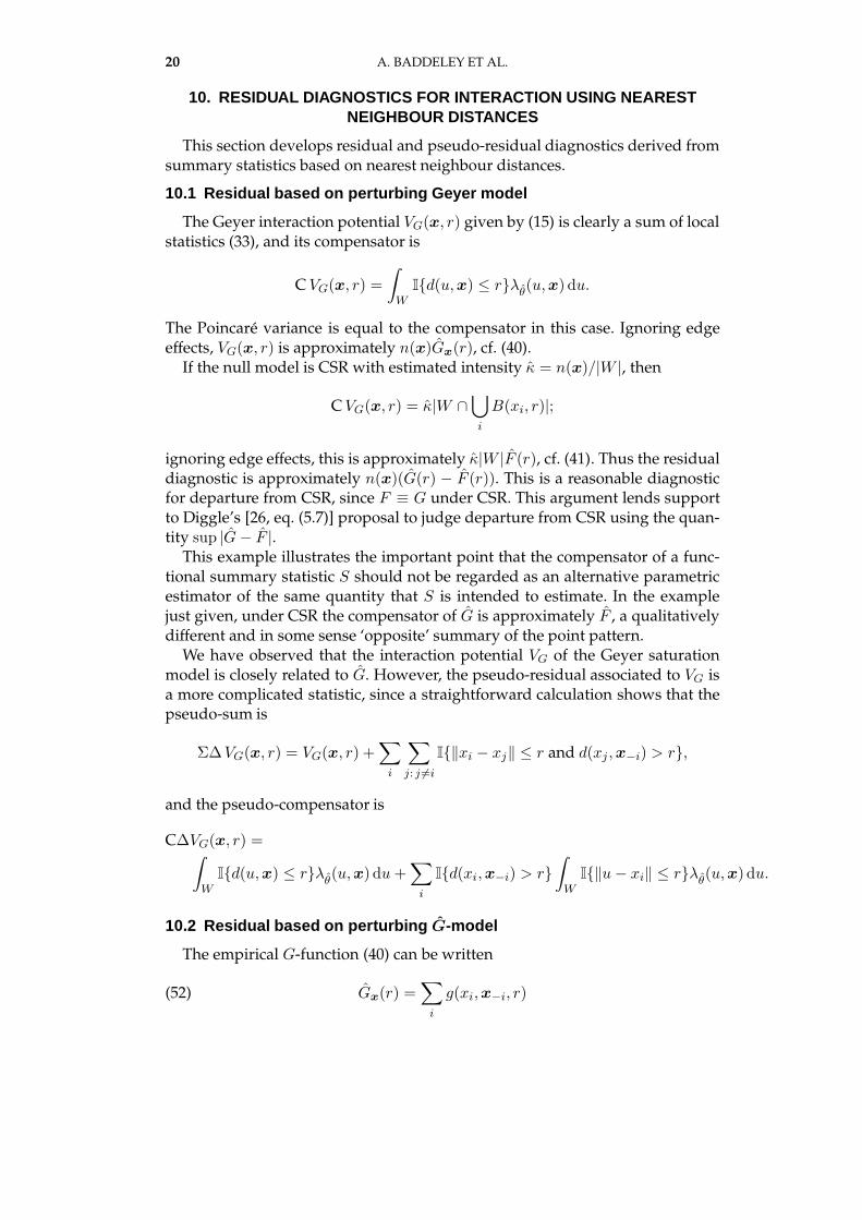
10.1 Residual based on perturbing Geyer model
The Geyer interaction potential VG(x, r) given by (15) is clearly a sum of localstatistics (33), and its compensator is
CVG(x, r) =
∫
WI{d(u,x) ≤ r}λθ(u,x) du.
The Poincare variance is equal to the compensator in this case. Ignoring edgeeffects, VG(x, r) is approximately n(x)Gx(r), cf. (40).
If the null model is CSR with estimated intensity κ = n(x)/|W |, then
CVG(x, r) = κ|W ∩⋃
i
B(xi, r)|;
ignoring edge effects, this is approximately κ|W |F (r), cf. (41). Thus the residualdiagnostic is approximately n(x)(G(r) − F (r)). This is a reasonable diagnosticfor departure from CSR, since F ≡ G under CSR. This argument lends supportto Diggle’s [26, eq. (5.7)] proposal to judge departure from CSR using the quan-tity sup |G− F |.
This example illustrates the important point that the compensator of a func-tional summary statistic S should not be regarded as an alternative parametricestimator of the same quantity that S is intended to estimate. In the examplejust given, under CSR the compensator of G is approximately F , a qualitativelydifferent and in some sense ‘opposite’ summary of the point pattern.
We have observed that the interaction potential VG of the Geyer saturationmodel is closely related to G. However, the pseudo-residual associated to VG isa more complicated statistic, since a straightforward calculation shows that thepseudo-sum is
Σ∆VG(x, r) = VG(x, r) +∑
i
∑
j: j 6=i
I{‖xi − xj‖ ≤ r and d(xj ,x−i) > r},
and the pseudo-compensator is
C∆VG(x, r) =∫
WI{d(u,x) ≤ r}λθ(u,x) du+
∑
i
I{d(xi,x−i) > r}∫
WI{‖u− xi‖ ≤ r}λθ(u,x) du.
10.2 Residual based on perturbing G-model
The empirical G-function (40) can be written
(52) Gx(r) =∑
i
g(xi,x−i, r)

GOODNESS-OF-FIT FOR SPATIAL POINT PROCESSES 21
where
(53) g(u,x, r) =1
n(x) + 1eG(u,x, r)I{d(u,x) ≤ r}, u 6∈ x
so that the Papangelou compensator of the empirical G-function is
C Gx(r) =
∫
Wg(u,x, r)λθ(u,x) du =
1
n(x) + 1
∫
W∩⋃i B(xi,r)eG(u,x, r)λθ(u,x) du.
The residual diagnostics obtained from the Geyer and G-models are very sim-ilar, and we choose to use the diagnostic based on the popular G-function. Aswith the K-function we typically use the compensator(s) of the fitted model(s)rather than the residual(s), to visually maintain the close connection to the em-pirical G-function.
The expressions for the pseudo-sum and pseudo-compensator of G are not ofsimple form, and we refrain from explicitly writing out these expressions. Forboth the G- and Geyer models, the pseudo-sum and pseudo-compensator arenot directly related to a well-known summary statistic. We prefer to plot thepseudo-residual rather than the pseudo-sum and pseudo-compensator(s).
11. DIAGNOSTICS FOR INTERACTION BASED ON EMPTY SPACEDISTANCES
11.1 Pseudo-residual based on perturbing area-interactio n model
When the perturbing model is the area-interaction process, it is convenient tore-parametrise the density, such that the canonical sufficient statistic VA given in(16) is re-defined as
VA(x, r) =1
|W | |W ∩⋃
i
B(xi, r)|.
This summary statistic is not naturally expressed as a sum of contributions fromeach point as in (33), so we shall only construct the pseudo-residual. Let
U(x, r) = W ∩⋃
i
B(xi, r).
The increment
∆uVA(x, r) =1
|W | (|U(x ∪ {u}, r)| − |U(x, r)|) , u 6∈ x
can be thought of as ‘unclaimed space’ — the proportion of space around thelocation u that is not “claimed” by the points of x. The pseudo-sum
Σ∆VA(x, r) =∑
i
∆xiVA(x, r)
is the proportion of the window that has ‘single coverage’ — the proportion oflocations in W that are covered by exactly one of the balls B(xi, r). This can beused in its own right as a functional summary statistic, and it corresponds to

22 A. BADDELEY ET AL.
a raw (i.e. not edge corrected) empirical estimate of a summary function F1(r)defined by
F1(r) = P (#{x ∈ X|d(u, x) ≤ r} = 1) ,
for any stationary point process X , where u ∈ R2 is arbitrary. Under CSR withintensity ρ we have
EF1(r) = ρπr2 exp(−ρπr2).
This summary statistic does not appear to be treated in the literature, and it maybe of interest to study it separately, but we refrain from a more detailed studyhere.
The pseudo-compensator corresponding to this pseudo-sum is
C∆VA(x, r) =
∫
W∆uVA(x, r)λθ(u,x) du.
This integral does not have a particularly simple interpretation even when thenull model is CSR.
11.2 Pseudo-residual based on perturbing F -model
Alternatively one could use a standard empirical estimator F of the emptyspace function F as the summary statistic in the pseudo-residual. The pseudo-sum associated with the perturbing F -model is
Σ∆ Fx(r) = n(x)Fx(r)−∑
i
Fx−i(r),
with pseudo-compensator
C∆ Fx(r) =
∫
W(Fx∪{u}(r)− Fx(r))λθ(u,x) du.
Ignoring edge correction weights, Fx∪{u}(r) − Fx(r) is approximately equal to∆uVA(x, r), so the pseudo-sum and pseudo-compensator associated with theperturbing F -model are approximately equal to the pseudo-sum and pseudo-compensator associated with the perturbing area-interaction model. Here, weusually prefer graphics using the pseudo-compensator(s) and the pseudo-sumsince this has an intuitive interpretation as explained above.
12. TEST CASE: TREND WITH INHIBITION
In sections 12–14 we demonstrate the diagnostics on the point pattern datasetsshown in Figure 1. This section concerns the synthetic point pattern in Figure 1b.
12.1 Data and models
Figure 1b shows a simulated realisation of the inhomogeneous Strauss pro-cess with first order term λ(x, y) = 200 exp(2x + 2y + 3x2), interaction rangeR = 0.05, interaction parameter γ = exp(φ) = 0.1 and W equal to the unitsquare, see (13) and (14). This is an example of extremely strong inhibition (neg-ative association) between neighbouring points, combined with a spatial trend.Since it is easy to recognise spatial trend in the data, (either visually or usingexisting tools such as kernel smoothing [27]) the main challenge here is to detectthe inhibition after accounting for the trend.

GOODNESS-OF-FIT FOR SPATIAL POINT PROCESSES 23
We fitted four point process models to the data in Figure 1b. They were (A)a homogeneous Poisson process (CSR); (B) an inhomogeneous Poisson processwith the correct form of the first order term, i.e. with intensity
(54) ρ(x, y) = exp(β0 + β1x+ β2y + β3x2)
where β0, . . . , β3 are real parameters; (C) a homogeneous Strauss process withthe correct interaction range R = 0.05; and (D) a process of the correct form,i.e. inhomogeneous Strauss with the correct interaction range R = 0.05 and thecorrect form of the first order potential (54).
12.2 Software implementation
The diagnostics defined in Sections 9–11 were implemented in the R lan-guage, and are publicly available11 in the spatstat library [5]. Unless other-wise stated, models were fitted by approximate maximum pseudo-likelihoodusing the algorithm of [4] with the default quadrature scheme in spatstat,having anm×m grid of dummy points wherem = max(25, 10[1+2
√n(x)/10])
was equal to 40 for most of our examples. Integrals over the domain W wereapproximated by finite sums over the quadrature points.
Somemodels were refitted using a finer grid of dummypoints, usually 80×80.The software also supports Huang-Ogata [36] one-step approximate maximumlikelihood.
12.3 Application of K diagnostics
12.3.1 Diagnostics for correct model First we fitted a point process model of thecorrect form (D). The fitted parameter values were β = (5.6,−0.46, 3.35, 2.05)and γ = 0.217 using the coarse grid of dummypoints, and β = (5.6,−0.64, 4.06, 2.44)and γ = 0.170 using the finer grid of dummy points, as against the true valuesβ = (5.29, 2, 2, 3) and γ = 0.1.
Figure 2 in Section 1 shows K along with its compensator for the fittedmodel,together with the theoretical K-function under CSR. The empirical K-functionand its compensator coincide very closely, suggesting correctly that the modelis a good fit. Figure 3a shows the residual K-function and the two-standard-deviation limits, where the surrogate standard deviation is the square root of(37). Figure 3b shows the corresponding standardised residual K-function ob-tained by dividing by the surrogate standard deviation.
Although this model is of the correct form, the standardised residual exceeds2 for small values of r. This is consistent with the prediction in Section 9.1.3that the test would be conservative for small r. For very small r there are small-sample effects so that a normal approximation to the null distribution of thestandardised residual is inappropriate.
Formal significance interpretation of the critical bands is limited, because thenull distribution of the standardised residual is not known exactly, and the val-ues ±2 are approximate pointwise critical values, i.e. critical values for the scoretest based on fixed r. The usual problems of multiple testing arise when the teststatistic is considered as a function of r: see [28, p. 14].
11. Note to editors/reviewers: software will be publicly released when the paper is acceptedfor publication.

24 A. BADDELEY ET AL.
0.00 0.02 0.04 0.06 0.08 0.10 0.12
−0.
006
−0.
004
−0.
002
0.00
00.
002
0.00
40.
006 Perfect fit
Critical bands
RK(r)
(a)
0.00 0.02 0.04 0.06 0.08 0.10 0.12
−3
−2
−1
01
23
4
Perfect fitCritical bands
TK(r)
(b)
Fig 3: Residual diagnostics based on pairwise distances, for a model of thecorrect form fitted to the data in Figure 1b. (a) residual K-function and two-standard-deviation limits under the fitted model of the correct form. (b) stan-dardised residual K-function under the fitted model of the correct form.
12.3.2 Comparison of competing models Figure 4a shows the empiricalK-functionand its compensator for each of the models (A)–(D) in Section 12.1. Figure 4bshows the corresponding residual plots, and Figure 4c the standardised residu-als. A positive or negative value of the residual suggests that the data are moreclustered or more inhibited, respectively, than the model. The clear inference isthat the Poisson models (A) and (B) fail to capture interpoint inhibition at ranger ≈ 0.05, while the homogeneous Strauss model (C) is less clustered than thedata at very large scales, suggesting that it fails to capture spatial trend. Thecorrect model (D) is judged to be a good fit.
The interpretation of this example requires some caution, because the residualK-function of the fitted Strauss models (C) and (D) is constrained to be approxi-mately zero at r = R = 0.05. The maximum pseudo-likelihood fitting algorithmsolves an estimating equation that is approximately equivalent to this constraint,because of (42).
It is debatable which of the presentations in Figure 4 is more effective at re-vealing lack-of-fit. A compensator plot such as Figure 4a seems best at captur-ing the main differences between competing models. It is particularly useful forrecognising a gross lack-of-fit. A residual plot such as Figure 4b seems betterfor making finer comparisons of goodness-of-fit, for example, assessing modelswith slightly different ranges of interaction. A standardised residual plot such asFigure 4c tends to be highly irregular for small values of r, due to discretisationeffects in the computation and the inherent nondifferentiability of the empiricalstatistic. In difficult cases we may apply smoothing to the standardised residual.
12.4 Application of G diagnostics
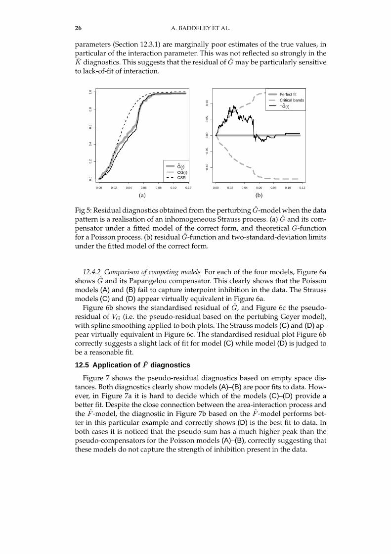
12.4.1 Diagnostics for correct model Consider again the model of the correctform (D). The residual and compensator of the empirical nearest neighbour func-tion G for the fitted model are shown in Figure 5. The residual plot suggests amarginal lack-of-fit for r < 0.025. This may be correct, since the fitted model

GOODNESS-OF-FIT FOR SPATIAL POINT PROCESSES 25
0.00 0.02 0.04 0.06 0.08 0.10 0.12
0.00
0.01
0.02
0.03
0.04
0.05
K(r)(A): CK(r)(B): CK(r)(C): CK(r)(D): CK(r)
(a)
0.00 0.02 0.04 0.06 0.08 0.10 0.12
−0.
005
0.00
00.
005
0.01
0 Perfect fit
(A): RK(r)(B): RK(r)(C): RK(r)(D): RK(r)
(b)
0.00 0.02 0.04 0.06 0.08 0.10 0.12
−5
05
Perfect fitCritical bands
(A): TK(r)(B): TK(r)(C): TK(r)(D): TK(r)
(c)
Fig 4: Goodness-of-fit diagnostics based on pairwise distances, for each of themodels (A)–(D) fitted to the data in Figure 1b. (a) K and its compensator undereach model. (b) residual K-function (empirical minus compensator) under eachmodel. (c) standardised residual K-function under each model.
26 A. BADDELEY ET AL.
parameters (Section 12.3.1) are marginally poor estimates of the true values, inparticular of the interaction parameter. This was not reflected so strongly in theK diagnostics. This suggests that the residual of Gmay be particularly sensitiveto lack-of-fit of interaction.
0.00 0.02 0.04 0.06 0.08 0.10 0.12
0.0
0.2
0.4
0.6
0.8
1.0
G(r)CG(r)CSR
(a)
0.00 0.02 0.04 0.06 0.08 0.10 0.12
−0.
10−
0.05
0.00
0.05
0.10
Perfect fitCritical bands
TG(r)
(b)
Fig 5: Residual diagnostics obtained from the perturbing G-modelwhen the datapattern is a realisation of an inhomogeneous Strauss process. (a) G and its com-pensator under a fitted model of the correct form, and theoretical G-functionfor a Poisson process. (b) residual G-function and two-standard-deviation limitsunder the fitted model of the correct form.
12.4.2 Comparison of competing models For each of the four models, Figure 6ashows G and its Papangelou compensator. This clearly shows that the Poissonmodels (A) and (B) fail to capture interpoint inhibition in the data. The Straussmodels (C) and (D) appear virtually equivalent in Figure 6a.
Figure 6b shows the standardised residual of G, and Figure 6c the pseudo-residual of VG (i.e. the pseudo-residual based on the pertubing Geyer model),with spline smoothing applied to both plots. The Strauss models (C) and (D) ap-pear virtually equivalent in Figure 6c. The standardised residual plot Figure 6bcorrectly suggests a slight lack of fit for model (C) while model (D) is judged tobe a reasonable fit.
12.5 Application of F diagnostics
Figure 7 shows the pseudo-residual diagnostics based on empty space dis-tances. Both diagnostics clearly showmodels (A)–(B) are poor fits to data. How-ever, in Figure 7a it is hard to decide which of the models (C)–(D) provide abetter fit. Despite the close connection between the area-interaction process andthe F -model, the diagnostic in Figure 7b based on the F -model performs bet-ter in this particular example and correctly shows (D) is the best fit to data. Inboth cases it is noticed that the pseudo-sum has a much higher peak than thepseudo-compensators for the Poisson models (A)–(B), correctly suggesting thatthese models do not capture the strength of inhibition present in the data.

GOODNESS-OF-FIT FOR SPATIAL POINT PROCESSES 27
0.00 0.02 0.04 0.06 0.08 0.10 0.12
0.0
0.2
0.4
0.6
0.8
1.0
G(r)(A): CG(r)(B): CG(r)(C): CG(r)(D): CG(r)
(a)
0.00 0.02 0.04 0.06 0.08 0.10 0.12
−4
−2
02
4
Perfect fitCritical bands
(A): TG(r)(B): TG(r)(C): TG(r)(D): TG(r)
(b)
0.00 0.02 0.04 0.06 0.08 0.10 0.12
−15
0−
100
−50
050
100
150
Perfect fit(A): R∆VG(r)(B): R∆VG(r)(C): R∆VG(r)(D): R∆VG(r)
(c)
Fig 6: Diagnostics based on nearest neighbour distances, for the models (A)–(D)fitted to the data in Figure 1b. (a) compensator for G. (b) smoothed standardisedresidual of G. (c) smoothed pseudo-residual derived from a perturbing Geyermodel.

28 A. BADDELEY ET AL.
0.00 0.02 0.04 0.06 0.08 0.10 0.12
0.0
0.1
0.2
0.3
0.4
∆VA(r)(A): C∆VA(r)(B): C∆VA(r)(C): C∆VA(r)(D): C∆VA(r)
(a)
0.00 0.02 0.04 0.06 0.08 0.10 0.12
0.0
0.1
0.2
0.3
0.4
0.5 ∆F(r)
(A): C∆F(r)(B): C∆F(r)(C): C∆F(r)(D): C∆F(r)
(b)
Fig 7: Pseudo-sumand pseudo-compensators for themodels (A)–(D) fitted to thedata in Figure 1b when the perturbing model is (a) the area-interaction process(null fitted on a fine grid) and (b) the F -model (null fitted on a coarse grid).
13. TEST CASE: CLUSTERING WITHOUT TREND
13.1 Data and models
Figure 1c is a realisation of a homogeneous Geyer saturation process [30] onthe unit square, with first order term λ = exp(4), saturation threshold s = 4.5and interaction parameters r = 0.05 and γ = exp(0.4) ≈ 1.5, i.e. the density is
(55) f(x) ∝ exp(n(x) log λ+ VG,s(x, r) log γ)
where
VG,s(x, r) =∑
i
min
s,
∑
j: j 6=i
I{‖xi − xj‖ ≤ r}
.
This is an example of moderately strong clustering (with interaction range R =2r = 0.1) without trend. The main challenge here is to correctly identify therange and type of interaction.
We fitted three point process models to the data: (E) a homogeneous Pois-son process (CSR); (F) a homogeneous area-interaction process with disc radiusr = 0.05; (G) a homogeneous Geyer saturation process of the correct form, withinteraction parameter r = 0.05 and saturation threshold s = 4.5 while the pa-rameters λ and γ in (55) are unknown. The parameter estimates for (G) werelog λ = 4.12 and log γ = 0.38.
13.2 Application of K diagnostics
A plot (not shown) of the K-function and its compensator, under each ofthe three models (E)–(G), demonstrates clearly that the homogeneous Poissonmodel (E) is a poor fit, but does not discriminate between the other models.
Figure 8 shows the residual K and the smoothed standardised residual K forthe three models. These diagnostics show that the homogeneous Poisson model(E) is a poor fit, with a positive residual suggesting correctly that the data are
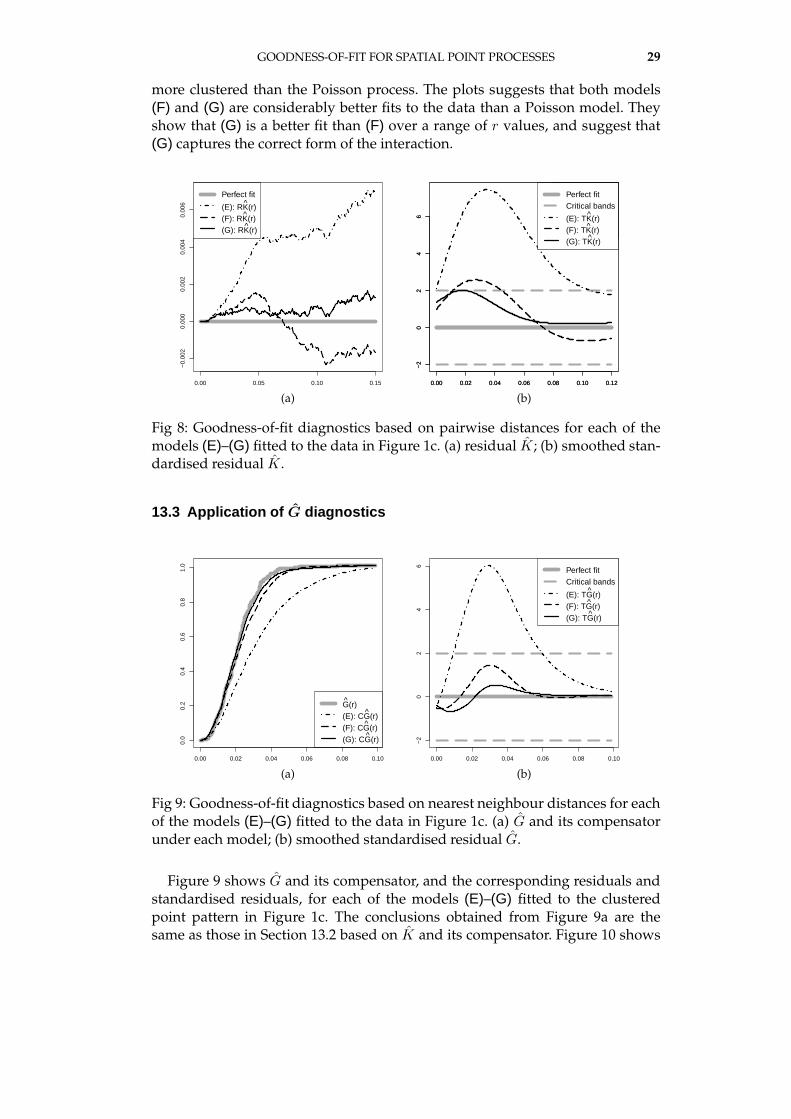
GOODNESS-OF-FIT FOR SPATIAL POINT PROCESSES 29
more clustered than the Poisson process. The plots suggests that both models(F) and (G) are considerably better fits to the data than a Poisson model. Theyshow that (G) is a better fit than (F) over a range of r values, and suggest that(G) captures the correct form of the interaction.
0.00 0.05 0.10 0.15
−0.
002
0.00
00.
002
0.00
40.
006
Perfect fit
(E): RK(r)(F): RK(r)(G): RK(r)
(a)
0.00 0.02 0.04 0.06 0.08 0.10 0.12
−2
02
46
Perfect fit
(E): TK(r)(F): TK(r)(G): TK(r)
0.00 0.02 0.04 0.06 0.08 0.10 0.12
−2
02
46
Perfect fitCritical bands
(E): TK(r)(F): TK(r)(G): TK(r)
(b)
Fig 8: Goodness-of-fit diagnostics based on pairwise distances for each of themodels (E)–(G) fitted to the data in Figure 1c. (a) residual K ; (b) smoothed stan-dardised residual K .
13.3 Application of G diagnostics
0.00 0.02 0.04 0.06 0.08 0.10
0.0
0.2
0.4
0.6
0.8
1.0
G(r)(E): CG(r)(F): CG(r)(G): CG(r)
(a)
0.00 0.02 0.04 0.06 0.08 0.10
−2
02
46
Perfect fitCritical bands
(E): TG(r)(F): TG(r)(G): TG(r)
(b)
Fig 9: Goodness-of-fit diagnostics based on nearest neighbour distances for eachof the models (E)–(G) fitted to the data in Figure 1c. (a) G and its compensatorunder each model; (b) smoothed standardised residual G.
Figure 9 shows G and its compensator, and the corresponding residuals andstandardised residuals, for each of the models (E)–(G) fitted to the clusteredpoint pattern in Figure 1c. The conclusions obtained from Figure 9a are thesame as those in Section 13.2 based on K and its compensator. Figure 10 shows

30 A. BADDELEY ET AL.
the smoothed pseudo-residual diagnostics based on the nearest neighbour dis-tances. The message from these diagnostics is very similar to that from Figure 9.
0.00 0.02 0.04 0.06 0.08 0.10
050
100
150
Perfect fit(E): R∆VG(r)(F): R∆VG(r)(G): R∆VG(r)
(a)
0.00 0.02 0.04 0.06 0.08 0.10
−0.
050.
000.
050.
100.
150.
200.
25
Perfect fit
(E): R∆G(r)(F): R∆G(r)(G): R∆G(r)
(b)
Fig 10: Smoothed pseudo-residuals for each of the models (E)–(G) fitted to theclustered point pattern in Figure 1c when the perturbing model is (a) Geyersaturation model with saturation 1, and (b) the G-model.
Models (F) and (G) have the same range of interaction R = 0.1. ComparingFigures 8 and 9 we might conclude that the G-compensator appears less sensi-tive to the form of interaction than the K-compensator. Other experiments sug-gest that G is more sensitive than K to discrepancies in the range of interaction.
13.4 Application of F diagnostics
Figure 11 shows the pseudo-residual diagnostics based on the empty spacedistances, for the three models fitted to the clustered point pattern in Figure 1c.In this case diagnostics based on the area-interaction process and the F -modelare very similar, as expected due to the close connection between the two diag-nostics. Here it is very noticeable that the pseudo-compensator for the Poissonmodel has a higher peak than the pseudo-sum, which correctly indicates thatthe data is more clustered than a Poisson process.
14. TEST CASE: JAPANESE PINES
14.1 Data and models
Figure 1a shows the locations of seedlings and saplings of Japanese blackpine, studied by Numata [52, 53] and analysed extensively by Ogata and Tane-mura [54, 55]. In their definitive analysis [55] the fitted model was an inhomo-geneous ‘soft core’ pairwise interaction process with log-cubic first order termλβ(x, y) = exp(Pβ(x, y)), where Pβ is a cubic polynomial in x and y with coeffi-cient vector β, and density
(56) f(β,σ2)(x) = c(β,σ2) exp
∑
i
Pβ(xi)−∑
i<j
(σ4/‖xi − xj‖4
)
where σ2 is a positive parameter.

GOODNESS-OF-FIT FOR SPATIAL POINT PROCESSES 31
0.00 0.02 0.04 0.06 0.08 0.10
0.0
0.1
0.2
0.3
0.4
0.5 ∆VA(r)
(E): C∆VA(r)(F): C∆VA(r)(G): C∆VA(r)
(a)
0.00 0.02 0.04 0.06 0.08 0.10
0.0
0.1
0.2
0.3
0.4 ∆F(r)
(E): C∆F(r)(F): C∆F(r)(G): C∆F(r)
(b)
Fig 11: Pseudo-sum and pseudo-compensators for the models (E)–(G) fitted tothe clustered point pattern in Figure 1c when the perturbing model is (a) area-interaction process and (b) the F -model.
Here we evaluate the goodness-of-fit of three models: (H) an inhomogeneousPoisson process with log-cubic intensity; (I) a homogeneous soft core pairwiseinteraction process, i.e. when Pβ(x, y) in (56) is replaced by a real parameter; (J)the Ogata-Tanemura model (56). For more detail on the dataset and the fittedinhomogeneous soft core model, see [55, 6].
A complication in this case is that the soft core process (56) is not Markov,since the pair potential c(u, v) = exp(−σ4/‖u − v‖4) is always positive. Nev-ertheless, since this function decays rapidly, it seems reasonable to apply theresidual and pseudo-residual diagnostics, using a cutoff distance R such that| log c(u, v)| ≤ ǫ when ‖u − v‖ ≤ R, for a specified tolerance ǫ. The cutoff de-pends on the fitted parameter value σ2. We chose ǫ = 0.0002 yielding R = 1.Estimated interaction parameters were σ2 = 0.11 for model (I) and σ2 = 0.12 formodel (J).
14.2 Application of K diagnostics
A plot (not shown) of K and its compensator for each of the models (H)–(J)suggests that the homogeneous soft core model (I) is inadequate, while the in-homogeneous models (H) and (J) are reasonably good fits to the data. Howeverit does not discriminate between the models (H) and (J).
Figure 12 shows smoothed version of the residual and standardised residualof K for each model. The Ogata-Tanemura model (J) is judged to be the best fit.
14.3 Application of G diagnostics
Finally, for each of the models (H)–(J) fitted to the Japanese pines data in Fig-ure 1a, Figure 13a shows G and its compensator. The conclusions are the sameas those based on K shown in Figure 12. Figure 14 shows the pseudo-residualswhen using either a perturbing Geyer model (Figure 14a) or a perturbing G-model (Figure 14b). Figures 14a-14b tell almost the same story: the inhomoge-neous Poisson model (H) provides the worst fit, while it is difficult to discrim-inate between the fit for the soft core models (I) and (J). In conclusion, consid-

32 A. BADDELEY ET AL.
0.0 0.5 1.0 1.5
−0.
10.
00.
10.
20.
30.
40.
5 Perfect fit
(H): RK(r)(I): RK(r)(J): RK(r)
(a)
0.0 0.5 1.0 1.5
−2
−1
01
23
Perfect fitCritical bands
(H): T∆K(r)(I): T∆K(r)(J): T∆K(r)
(b)
Fig 12: Goodness-of-fit diagnostics based on pairwise distances for each of themodels (H)–(J) fitted to the Japanese pines data in Figure 1a. (a) smoothed resid-ual K ; (b) smoothed standardised residual K .
ering Figures 12, 13 and 14, the Ogata-Tanemura model (J) provides the bestfit.
14.4 Application of F diagnostics
Finally, the empty space pseudo-residual diagnostics are shown in Figure 15for the Japanese Pines data in Figure 1a. This gives a clear indication that theOgata-Tanemura model (J) is the best fit to the data, and the data pattern ap-pears to be too regular compared to the Poisson model (H) and not regularenough for the homogeneous softcore model (I).
15. SUMMARY OF TEST CASES
In this section we discuss which of the diagnostics we prefer to use based ontheir behaviour for the three test cases in Sections 12-14.
Typically the various diagnostics supplement each other well, and it is recom-mended to use more than one diagnostic when judging goodness-of-fit. Com-pensator and pseudo-compensator plots are informative for gaining an overallpicture of goodness-of-fit, and tend to make it easy to recognize a poor fit whencomparing competing models. To compare models which fit closely, it may bemore informative to use (standardised) residuals or pseudo-residuals. We pre-fer to use the standardised residuals, but it is important not to over-interpret thesignificance of departure from zero.
Based on the test cases here, it is not clear whether diagnostics based on pair-wise distances, nearest neighbour distances, or empty space distances are prefer-able. However, for each of thesewe prefer to workwith compensators and resid-uals rather than pseudo-compensators and pseudo-residuals when possible (i.e.it is only necessary to use pseudo-versions for diagnostics based on empty spacedistances). For instance, for the first test case (Section 12) the best compensatorplot is that in Figure 4a based on pairwise distances (K and C K) which makesit easy to identify the correct model. On the other hand in this test case the best

GOODNESS-OF-FIT FOR SPATIAL POINT PROCESSES 33
0.0 0.2 0.4 0.6 0.8 1.0
0.0
0.2
0.4
0.6
0.8
1.0
G(r)(H): CG(r)(I): CG(r)(J): CG(r)
(a)
0.0 0.2 0.4 0.6 0.8 1.0
−0.
06−
0.04
−0.
020.
000.
020.
04
Perfect fit
(H): RG(r)(I): RG(r)(J): RG(r)
(b)
0.0 0.2 0.4 0.6 0.8 1.0
−2
−1
01
2
G(r)Critical bands
(H): CG(r)(I): CG(r)(J): CG(r)
(c)
Fig 13: Goodness-of-fit diagnostics based on nearest neighbour distances foreach of the models (H)–(J) fitted to the Japanese pines data in Figure 1a. (a) Gand its compensator; (b) smoothed residual G; (c) smoothed standardised resid-ual G.

34 A. BADDELEY ET AL.
0.0 0.2 0.4 0.6 0.8 1.0
−50
−40
−30
−20
−10
0
Perfect fit(H): R∆VG(r)(I): R∆VG(r)(J): R∆VG(r)
(a)
0.0 0.2 0.4 0.6 0.8 1.0
−0.
20−
0.15
−0.
10−
0.05
0.00
Perfect fit
(H): R∆G(r)(I): R∆G(r)(J): R∆G(r)
(b)
Fig 14: Smoothed pseudo-residuals for each of the models (H)–(J) fitted to theJapanese pines data in Figure 1a when the perturbing model is (a) Geyer satura-tion model with saturation 1 (null fitted on a fine grid) and (b) the G-model.
0.0 0.2 0.4 0.6 0.8 1.0 1.2
0.0
0.1
0.2
0.3
0.4
∆VA(r)(H): C∆VA(r)(I): C∆VA(r)(J): C∆VA(r)
(a)
0.0 0.2 0.4 0.6 0.8 1.0 1.2
0.00
0.05
0.10
0.15
0.20
0.25
0.30 ∆F(r)
(H): C∆F(r)(I): C∆F(r)(J): C∆F(r)
(b)
Fig 15: Pseudo-sum and pseudo-compensators for the models (H)–(J) fittedto the real data pattern in Figure 1a when the perturbing model is (a) area-interaction process and (b) the F -model.

GOODNESS-OF-FIT FOR SPATIAL POINT PROCESSES 35
residual type plot is that in Figure 6b based on nearest neighbour distances (T G)where the correct model is the only one within the critical bands. However, inthe third test case (Section 14) the best compensator plot is one of the plots inFigure 15 with pseudo-compensators based on empty space distances (Σ∆VA
and C∆VA respectively Σ∆ F and C∆ F ) which clearly indicates which modelis correct.
In the first and third test cases (Sections 12 and 14), which both involve inho-mogeneous models, it is clear that K and its compensator are more sensitive tolack of fit in the first order term than G and its compensator (compare e.g. theresults for the homogeneous model (C) in Figures 4a and 6a). It is our generalexperience that diagnostics based on K are particularly well suited to assess thepresence of interaction and to identify the general form of interaction. Diagnos-tics based on K and in particular on G seem to be good for assessing the rangeof interaction.
Finally, it is worth mentioning the computational difference between the var-ious diagnostics (timed on a 2.5 GHz laptop). The calculations for K and C Kused in Figure 2 are carried out in approximately five seconds whereas the cor-responding calculations for G and C G only take a fraction of a second. For e.g.Σ∆ F and C∆ F the calculations take about 45 seconds.
ACKNOWLEDGMENTS
This paper has benefited from very fruitful discussions with Professor Ras-mus P. Waagepetersen. The research was supported by The University of West-ernAustralia, theDanishNatural Science ResearchCouncil (grants 272-06-0442and 09-072331,Point process modelling and statistical inference), theDanish Agencyfor Science, Technology and Innovation (grant 645-06-0528, International Ph.D.student) and by the Centre for Stochastic Geometry and Advanced Bioimaging,funded by a grant from the Villum Foundation.
REFERENCES
[1] ALM, S. E. (1988). Approximation and Simulation of the Distributions of Scan Statistics forPoisson Processes in Higher Dimensions. Extremes 1 111–126.
[2] ATKINSON, A. C. (1982). Regression diagnostics, transformations and constructed variables(with discussion). J. R. Statist. Soc. Ser. B Stat. Methodol. 44 1–36.
[3] BADDELEY, A., MØLLER, J. and PAKES, A. G. (2008). Properties of residuals for spatial pointprocesses. Ann. Inst. Statist. Math. 60 627–649.
[4] BADDELEY, A. and TURNER, R. (2000). Practical maximum pseudolikelihood for spatial pointpatterns (with discussion). Aust. N. Z. J. Stat. 42 283–322.
[5] BADDELEY, A. and TURNER, R. (2005). Spatstat: an R package for analyzing spatial pointpatterns. J. Statist. Software 12 1–42. URL: www.jstatsoft.org, ISSN: 1548-7660.
[6] BADDELEY, A., TURNER, R., MØLLER, J. and HAZELTON, M. (2005). Residual analysis forspatial point processes (with discussion). J. R. Statist. Soc. Ser. B Stat. Methodol. 67 617–666.
[7] BADDELEY, A. J. (1980). A limit theorem for statistics of spatial data. Adv. in Appl. Probab. 12447–461.
[8] BADDELEY, A. J. (1993). Stereology and Survey Sampling Theory. Bull. Int. Statist. Inst. 50,book 2 435–449.
[9] BADDELEY, A. J. (1999). Spatial sampling and censoring. In Stochastic Geometry: Likelihood andComputation (O. E. Barndorff-Nielsen,W. S. Kendall and M. N. M. van Lieshout, eds.) 2 37–78.Chapman and Hall, London.
[10] BADDELEY, A. J. and MØLLER, J. (1989). Nearest-neighbour Markov point processes andrandom sets. Int. Stat. Rev. 57 89–121.

36 A. BADDELEY ET AL.
[11] BADDELEY, A. J. and VAN LIESHOUT, M. N. M. (1995). Area-interaction point processes.Ann. Inst. Statist. Math. 47 601–619.
[12] BARNARD, G. (1963). Contribution to discussion of “The spectral analysis of point pro-cesses” by M.S. Bartlett. J. R. Statist. Soc. Ser. B Stat. Methodol. 25 294.
[13] BERMAN, M. (1986). Testing for spatial association between a point process and anotherstochastic process. J. Roy. Statist. Soc. Ser. C. 35 54–62.
[14] BESAG, J. (1978). Some methods of statistical analysis for spatial data. Bull. Int. Statist. Inst.44 77–92.
[15] CHEN, C. (1983). Score tests for regressionmodels. J. Amer. Statist. Assoc. 78 158–161.
[16] CHETWYND, A. G. and DIGGLE, P. J. (1998). On estimating the reduced second momentmeasure of a stationary spatial point process. Aust. N. Z. J. Stat. 40 11–15.
[17] CONNIFFE, D. (2001). Score tests when a nuisance parameter is unidentified under the nullhypothesis. J. Statist. Plann. Inference 97 67–83.
[18] COOK, R. D. and WEISBERG, S. (1983). Diagnostics for heteroscedasticity in regression.Biometrika 70 1–10.
[19] CORDY, C. B. (1993). An extension of the Horvitz-Thompson theorem to point samplingfrom a continuous universe. Statist. Probab. Lett. 18 353–362.
[20] COX, D. R. (1972). The statistical analysis of dependencies in point processes. In StochasticPoint Processes (P. A. W. Lewis, ed.) 55–66. Wiley, New York.
[21] COX, D. R. and HINKLEY, D. V. (1974). Theoretical statistics. Chapman and Hall, London.
[22] CRESSIE, N. A. C. (1991). Statistics for Spatial Data. John Wiley and Sons, New York.
[23] DALEY, D. J. and VERE-JONES, D. (1988). An Introduction to the Theory of Point Processes.Springer Verlag, New York.
[24] DAVIES, R. B. (1977). Hypothesis testing when a nuisance parameter is present only underthe alternative. Biometrika 64 247–254.
[25] DAVIES, R. B. (1987). Hypothesis testing when a nuisance parameter is present only underthe alternative. Biometrika 74 33–43.
[26] DIGGLE, P. J. (1979). On parameter estimation and goodness-of-fit testing for spatial pointpatterns. Biometrika 35 87–101.
[27] DIGGLE, P. J. (1985). A kernel method for smoothing point process data. J. Roy. Statist. Soc.Ser. C. 34 138–147.
[28] DIGGLE, P. J. (2003). Statistical Analysis of Spatial Point Patterns, Second ed. Hodder Arnold,London.
[29] GEORGII, H. O. (1976). Canonical and grand canonical Gibbs states for continuum systems.Comm. Math. Phys. 48 31–51.
[30] GEYER, C. J. (1999). Likelihood Inference for Spatial Point Processes. In Stochastic Geometry:Likelihood and Computation, (O. E. Barndorff-Nielsen,W. S. Kendall andM. N.M. van Lieshout,eds.). Monographs on Statistics and Applied Probability 80 3 79–140. Chapman and Hall / CRC,Boca Raton, Florida.
[31] HANISCH, K. (1984). Some remarks on estimators of the distribution function of nearestneighbour distance in stationary spatial point patterns. Math. Operationsforsch. Statist. Ser.Statist. 15 409–412.
[32] HANSEN, B. E. (1996). Inference when a nuisance parameter is not identified under the nullhypothesis. Econometrica 64 413–430.
[33] HEINRICH, L. (1988). Asymptotic behaviour of an empirical nearest-neighbour distancefunction for stationary Poisson cluster processes.Math. Nachr. 136 131–148.
[34] HEINRICH, L. (1988). Asymptotic Gaussianity of some estimators for reduced factorial mo-ment measures and product densities of stationary Poisson cluster processes. Statistics 19 87–106.
[35] HOPE, A. C. A. (1968). A simplified Monte Carlo significance test procedure. J. R. Statist.Soc. Ser. B Stat. Methodol. 30 582–598.
[36] HUANG, F. and OGATA, Y. (1999). Improvements of the maximum pseudo-likelihood esti-mators in various spatial statistical models. J. Comput. Graph. Statist. 8 510–530.
[37] ILLIAN, J., PENTTINEN, A., STOYAN, H. and STOYAN, D. (2008). Statistical Analysis and Mod-elling of Spatial Point Patterns. John Wiley and Sons, Chichester.

GOODNESS-OF-FIT FOR SPATIAL POINT PROCESSES 37
[38] JENSEN, J. L. and MØLLER, J. (1991). Pseudolikelihood for exponential family models ofspatial point processes. Ann. Appl. Probab. 1 445–461.
[39] JOLIVET, E. (1980). Central limit theorem and convergence of empirical processes for sta-tionary point processes. In Point processes and queueing problems (P. Bastfai and J. Tomko, eds.)117–161. North-Holland, Amsterdam.
[40] KALLENBERG, O. (1978). On conditional intensities of point processes. Z. Wahrscheinlichkeit.41 205–220.
[41] KALLENBERG, O. (1984). An informal guide to the theory of conditioning in point processes.Int. Stat. Rev. 52 151–164.
[42] KELLY, F. P. and RIPLEY, B. D. (1976). A note on Strauss’s model for clustering. Biometrika 63357–360.
[43] KULLDORFF, M. (1999). Spatial scan statistics: models, calculations, and applications. InRecent Advances on Scan Statistics (J. Glaz and N. Balakrishnan, eds.) 303–322. Birkhauser,Boston.
[44] KUTOYANTS, Y. A. (1998). Statistical Inference for Spatial Poisson Processes. Lecture Notes inStatistics 134. Springer, New York.
[45] LAST, G. and PENROSE, R. (2010). Poisson process Fock space representation, chaos expan-sion and covariance inequalities. Manuscript in preparation.
[46] LAWSON, A. B. (1993). On the analysis of mortality events around a prespecified fixed point.J. Roy. Statist. Soc. Ser. A 156 363-377.
[47] LOTWICK, H. W. and SILVERMAN, B. W. (1982). Methods for analysing spatial processes ofseveral types of points. J. R. Statist. Soc. Ser. B Stat. Methodol. 44 406–413.
[48] MØLLER, J., SYVERSVEEN, A. R. and WAAGEPETERSEN, R. (1998). Log Gaussian Cox pro-cesses. Scand. J. Statist. 25 451-482.
[49] MØLLER, J. and WAAGEPETERSEN, R. P. (2007). Modern spatial point processmodelling andinference (with discussion). Scand. J. Statist. 34 643–711.
[50] MØLLER, J. and WAAGEPETERSEN, R. P. (2004). Statistical Inference and Simulation for SpatialPoint Processes. Chapman and Hall/CRC, Boca Raton.
[51] NGUYEN, X. X. and ZESSIN, H. (1979). Integral and differential characterizations of Gibbsprocesses.Math. Nachr. 88 105–115.
[52] NUMATA, M. (1961). Forest vegetation in the vicinity of Choshi — coastal flora and veg-etation at Choshi, Chiba prefecture, IV (in Japanese). Bull. Choshi Mar. Lab. 3 28–48. ChibaUniversity.
[53] NUMATA, M. (1964). Forest vegetation, particularly pine stands in the vicinity of Choshi —flora and vegetation in Choshi, Chiba prefecture, VI (in Japanese). Bull. Choshi Mar. Lab. 627–37. Chiba University.
[54] OGATA, Y. and TANEMURA, M. (1981). Estimation of interaction potentials of spatial pointpatterns through the maximum likelihood procedure. Ann. Inst. Statist. Math. B 33 315–338.
[55] OGATA, Y. and TANEMURA, M. (1986). Likelihood estimation of interaction potentialsand external fields of inhomogeneous spatial point patterns. In Pacific Statistical Congress(I. S. FRANCIS, B. J. F. MANLY and F. C. LAM, eds.) 150–154. Elsevier, Amsterdam.
[56] OHSER, J. (1983). On estimators for the reduced secondmoment measure of point processes.Math. Operationsforsch. Statist. Ser. Statist. 14 63–71.
[57] OHSER, J. and STOYAN, D. (1981). On the second-order and orientation analysis of planarstationary point processes. Biom. J. 23 523-533.
[58] PAPANGELOU, F. (1974). The conditional intensity of general point processes and an appli-cation to line processes. Z. Wahrscheinlichkeit. 28 207–226.
[59] PREGIBON, D. (1982). Score tests in GLIM with applications. In GLIM 82: Proceedings of theInternational Conference on Generalized Linear Models. Lecture Notes in Statistics 14. Springer,New York.
[60] RAO, C. R. (1948). Large sample tests of statistical hypotheses concerning several parameterswith applications to problems of estimation. Math. Proc. Cambridge Philos. Soc. 44 50–57.
[61] RATHBUN, S. L. and CRESSIE, N. (1994). Asymptotic properties of estimators of the param-eters of spatial inhomogeneous Poisson point processes. Adv. in Appl. Probab. 26 122–154.
[62] RIPLEY, B. D. (1976). The second-order analysis of stationary point processes. J. Appl. Probab.13 255–266.

38 A. BADDELEY ET AL.
[63] RIPLEY, B. D. (1977). Modelling spatial patterns (with discussion). J. R. Statist. Soc. Ser. B Stat.Methodol. 39 172–212.
[64] RIPLEY, B. D. (1988). Statistical Inference for Spatial Processes. Cambridge University Press.
[65] RIPLEY, B. D. and KELLY, F. P. (1977). Markov point processes. J. Lond. Math. Soc. 15 188-192.
[66] SCHLADITZ, K. and BADDELEY, A. J. (2000). A third order point process characteristic. Scand.J. Statist. 27 657–671.
[67] SILVAPULLE, M. (1996). A test in the presence of nuisance parameters. J. Amer. Statist. Assoc.91 1690–1693.
[68] STILLINGER, F. H., STILLINGER, D. K., TORQUATO, S., TRUSKETT, T. M. andDEBENEDETTI, P. G. (2000). Triangle distribution and equation of state for classical rigid disks.J. Stat. Phys. 100 49–72.
[69] STOYAN, D., KENDALL, W. S. and MECKE, J. (1987). Stochastic Geometry and its Applications.John Wiley and Sons, Chichester.
[70] STOYAN, D. and STOYAN, H. (1995). Fractals, Random Shapes and Point Fields. John Wiley andSons, Chichester.
[71] STRAUSS, D. J. (1975). A model for clustering. Biometrika 63 467–475.
[72] VAN LIESHOUT, M. N. M. (2000). Markov Point Processes and their Applications. Imperial Col-lege Press, London.
[73] WALD, A. (1941). Some examples of asymptotically most powerful tests. Ann. Math. Statist.12 396–408.
[74] WALLER, L., TURNBULL, B., CLARK, L. C. and NASCA, P. (1992). Chronic Disease Surveil-lance and testing of clustering of disease and exposure: Application to leukaemia incidenceand TCE-contaminated dumpsites in upstate New York. Environmetrics 3 281–300.
[75] WANG, P. C. (1985). Adding a variable in generalized linear models. Technometrics 27 273–276.
[76] WIDOM, B. and ROWLINSON, J. S. (1970). New model for the study of liquid-vapor phasetransitions. J. Chem. Phys. 52 1670–1684.
[77] WU, L. (2000). A new modified logarithmic Sobolev inequality for Poisson point processesand several applications. Probab. Theory Related Fields 118 427–438.

GOODNESS-OF-FIT FOR SPATIAL POINT PROCESSES 39
APPENDIX A: FURTHER DIAGNOSTICS
In this appendixwe present other diagnostics whichwe have not implementedin software. The examples are therefore not accompanied by experimental re-sults.
A.1 Third and higher order functional summary statistics
While the intensity and K-function are frequently-used summaries for thefirst and second order moment properties of a spatial point process, third andhigher order summaries have been less used, though various such summarieshave been suggested in e.g. [66, 48, 68, 70].
Statistic of order k For a functional summary statistic of k-th order, say
(57) S(x, r) =∑
{xi1,...,xik
}⊆x
q({xi1 , . . . , xik}, r)
we obtain
(58) Σ∆S(x, r) = k!S(x, r) = k!∑
{xi1,...,xik
}⊆x
q({xi1 , . . . , xik}, r)
(59)
C∆S(x, r) = k!CS(x, r) = (k − 1)!
∫
W
∑
{xi1,...,xik−1
}⊆x
q({xi1 , . . . , xik−1, u}, r)λθ(u,x) du
(60) PU(θ, r) = k!RS(x, r) = k!S(x, r)− k!CS(x, r)
where i1, i2, . . . are pairwise distinct in the sums in (58)-(59). So in this case again,pseudo-residual diagnostics are equivalent to those based on residuals.
Third order example For a stationary and isotropic point process (i.e., whenthe distribution of X is invariant under translations and rotations), the inten-sity and K-function of the process completely determine its first and secondorder moment properties. However, even in this case, the simplest descriptionof third order moments depends on a three-dimensional vector specified fromtriplets (xi, xj , xk) of points from X such as the lengths and angle between thevectors xi − xj and xj − xk. This is often considered too complex, and insteadone considers a certain one-dimensional property of the triangle T (xi, xj , xk) asexemplified below, where L(xi, xj , xk) denotes the largest side in T (xi, xj, xk).
Let the canonical sufficient statistic of the perturbing density (27) be
(61) S(x, r) = VT (x, r) =∑
i<j<k
I(L(xi, xj , xk) ≤ r).
The perturbing model is a special case of the triplet interaction point process stud-ied in [30]. It is also a special case of (57) with
q({xi, xj , xk}, r) = I(L(xi, xj , xk) ≤ r)
and so residual and pseudo-residual diagnostics are equivalent and given by(58)-(60).

40 A. BADDELEY ET AL.
A.2 Tessellation functional summary statistics
Some authors have suggested the use of tessellation methods for characteriz-ing spatial point processes; see [37] and the references therein. A planar tessella-tion is a subdivision of planar region such as W or the entire plane R2.
For example, consider the Dirichlet tessellation of W generated by x, that is,the tessellation with cells
C(xi|x) = {u ∈ W | ‖u− xi‖ ≤ ‖u− xj‖ for all xj in x}, i = 1, . . . , n.
Suppose the canonical sufficient statistic of the perturbing density (27) is
(62) S(x, r) = VO(x, r) =∑
i
I(|C(xi|x)| ≤ r).
This is a sum of local contributions as in (33), although not of local statisticsin the sense mentioned in Section 6.3, since I(|C(xi|x)| ≤ r) depends on thosepoints in x−i which are Dirichlet neighbours to xi and such points may of coursenot be r-close to xi (unless r is larger than the diameter of W ). We call this per-turbing model for a soft Ord’s process; Ord’s process as defined in [10] is the lim-iting case φ → −∞ in (27), i.e. when r is the lower bound on the size of cells.Since VO(x) ≤ n(x), the perturbing model is well-defined for all φ ∈ R.
Let ∼x denote the Dirichlet neighbour relation for the points in x, that is,xi ∼x xj if C(xi|x) ∩ C(xj|x) 6= ∅. Note that xi ∼x xi. Now,
∆uS(x, r) =I(|C(u|x ∪ {u})| ≤ r)
+∑
v 6=u: v∼x∪{u}u
[I(|C(v|x ∪ {u})| ≤ r)− I(|C(v|x \ {u})| ≤ r)](63)
depends not only on the points in x which are Dirichlet neighbours to u (withrespect to ∼x∪{u}) but also on the Dirichlet neighbours to those points (withrespect to ∼x∪{u} or with respect to ∼x\{u}). In other words, if we define theiterated Dirichlet neighbour relation by that xi ∼2
x xj if there exists some xksuch that xi ∼x xk and xj ∼x xk, then t(u,x) depends on those points in xwhichare iterated Dirichlet neighbours to u with respect to ∼x∪{u} or with respect to∼x\{u}. The pseudo-sum associated to the soft Ord’s process is
Σ∆VO(x, r) = VO(x, r) +∑
i
∑
j 6=i:xj∼xxi
[I(|C(xj |x)| ≤ r)− I(|C(xj |x−i)| ≤ r))]
and from (29) and (63) we obtain the pseudo-compensator. From (36) and (62),we obtain the Papangelou compensator
CVO(x, r) =
∫
WI(|C(u|x ∪ {u})| ≤ r)λθ(u,x) du.
Many other examples of tessellation characteristics may be of interest. Forexample, often the Delaunay tessellation is used instead of the Dirichlet tessella-tion. This is the dual tessellation to the Dirichlet tessellation, where the Delaunaycells generated by x are given by those triangles T (xi, xj, xk) such that the disccontaining xi, xj , xk in its boundary does not contain any further points from

GOODNESS-OF-FIT FOR SPATIAL POINT PROCESSES 41
x (strictly speaking we need to assume a regularity condition, namely that xhas to be in general quadratic position; for such details, see [10]. For instance,the summary statistic t(x, r) given by the number of Delaunay cells T (xi, xj , xk)with L(xi, xj , xk) ≤ r is related to (61) but concerns only the maximal cliques ofDirichlet neighbours (assuming again the general quadratic position condition).The corresponding perturbing model has to the best of our knowledge not beenstudied in the literature.
APPENDIX B: VARIANCE FORMULAE
This Appendix concerns the variance of diagnostic quantities of the form
I =∑
i
h(xi,X−i)−∫
Wh(u,x)λθ(u,X) du
R =∑
i
h(xi,X−i)−∫
Wh(u,x)λθ(u,X) du
where h(·) is a functional for which these quantities are almost surely finite, Xis a point process on W with conditional intensity λθ(u,X) and θ is an estimateof θ (e.g. the MPLE).
B.1 General identity
Exact formulae for the variance of the innovation I and residual R are givenin [3]. Expressions for VarR are unwieldy [3, Sect. 6], but to a first approxima-tion we may ignore the effect of estimating θ and consider the variance of I .Suppressing the dependence on θ, this is [3, Prop. 4]
VarI =
∫
WE[h(u,X)2λ(u,X)
]du
+
∫
W
∫
WE [A(u, v,X) +B(u, v,X)] dudv(64)
where
A(u, v,X) = ∆uh(v,X)∆vh(u,X)λ2(u, v,X)
B(u, v,X) = h(u,X)h(v,X) {λ2(u, v,X)− λ(u,X)λ(v,X)}
where λ2(u, v,x) = λ(u,x)λ(v,x∪{u}) is the second order conditional intensity.Note that for a Poisson process B(u, v,X) is identically zero since λ(u,X) =λ(u).
B.2 Pseudo-score
Let S(x, z) be a functional summary statistic with function argument z. Takeh(u,X) = ∆uS(x, z). Then the innovation I is the pseudo-score (23), and thevariance formula (64) becomes
Var [PU(θ)] =
∫
WE[(∆uS(X , z))2 λ(u,X)
]du
+
∫
W
∫
WE[(∆u∆vS(X , z))2 λ2(u, v,X)
]dudv
+
∫
W
∫
WE [∆uS(x, z)∆vS(x, z) {λ2(u, v,X)− λ(u,X)λ(v,X)}] dudv(65)

42 A. BADDELEY ET AL.
where for u 6= v and {u, v} ∩ x = ∅,
∆u∆vS(x, z) = ∆v∆uS(x, z) = S(x∪{u, v}, z)−S(x∪{u}, z)−S(x∪{v}, z)+S(x, z).
APPENDIX C: MODIFIED EDGE CORRECTIONS
Appendices C–E describe modifications to the standard edge corrected esti-mators of K(r) and G(r) that are required in the conditional case (Section 2.3)because the Papangelou conditional intensity λ(u,x) can or should only be eval-uated at locations u ∈ W ◦ whereW ◦ ⊂ W . The corresponding compensators arealso given.
Assume the point process is Markov and we are in the conditional case asdescribed in Section 5.4. Consider an empirical functional statistic of the form
(66) SW (x, r) =∑
xi∈xsW (xi,x \ {xi}, r)
with compensator (in the unconditional case)
CSW (x, r) =
∫
WsW (u,x, r)λθ(u,x) du.
We explore two different strategies for modifying the edge correction.In the restriction approach, we replaceW byW ◦ and x by x◦ = x∩W ◦ yielding
SW ◦(x, r) =∑
xi∈x◦sW ◦(xi,x
◦ \ {xi}, r)(67)
CSW ◦(x, r) =
∫
W ◦sW ◦(u,x◦, r)λθ(u,x
◦ | x+) du.
In this approach, data points in the boundary regionW+ are ignored in the cal-culation of the empirical statistic S. The boundary configuration x+ = x ∩W+
contributes only to the estimation of θ and the calculation of the conditional in-tensity λθ(·, · | x+). This has the advantage that the modified empirical statistic(67) is identical to the standard statistic S computed on the subdomain W ◦; itcan be computed using existing software, and requires no new theoretical justi-fication.
The disadvantage of the restriction approach is that we lose information bydiscarding some of the data. In the reweighting approach we retain the boundarypoints and compute
SW ◦,W (x, r) =∑
xi∈x◦sW ◦,W (xi,x \ {xi}, r)
CSW ◦,W (x, r) =
∫
W ◦sW ◦,W (u,x, r)λθ(u,x
◦ | x+) du
where sW ◦,W (·) is a modified version of sW (·). Thus, boundary points contributeto the computation of the modified summary statistic SW ◦,W and its compen-sator. The modification is designed so that SW ◦,W has properties analogous toSW .

GOODNESS-OF-FIT FOR SPATIAL POINT PROCESSES 43
The K-function and G-function of a point process Y in R2 is defined [62, 63]under the assumption that Y is second-order stationary. The standard estima-tors KW (r) respectively Gx(r) of the K-function and G-function are designedto be approximately pointwise unbiased estimators of K(r) respectively G(r)when applied toX = Y ∩W .
We do not necessarily assume stationarity, but when constructing modifiedsummary statistics KW ◦,W (r) and GW ◦,W (r), we shall require that they are alsoapproximately pointwise unbiased estimators of K(r) respectively G(r) whenY is stationary. This greatly simplifies the interpretation of plots of KW ◦,W (r)
and GW ◦,W (r) and their compensators.
APPENDIX D: MODIFIED EDGE CORRECTIONS FOR THE K-FUNCTION
D.1 Horvitz-Thompson estimators
The most common nonparametric estimators of theK-function [62, 56, 9] arecontinuous Horvitz-Thompson type estimators [8, 19] of the form
(68) K(r) = KW (r) =1
ρ2(x)|W |∑
i 6=j
eW (xi, xj)I{‖xi − xj‖ ≤ r}.
Here ρ2 = ρ2(x) should be an approximately unbiased estimator of the squared
intensity ρ2 for stationary processes. Usually ρ2(x) = n(n − 1)/|W |2 where n =n(x).
The term eW (u, v) is an edge correction weight, depending on the geometry
of W , designed so that the double sum in (68), say Y (r) = ρ2(x)|W |K(r), isan unbiased estimator of Y (r) = ρ2|W |K(r). Popular examples are the Ohser-Stoyan translation edge correction with
(69) eW (u, v) = etransW (u, v) =|W |
|W ∩ (W + (u− v))|and Ripley’s isotropic correction with
(70) eW (u, v) = eisoW (u, v) =2π||u − v||
length(∂B(u, ||u − v||) ∩W ).
Estimators of the form (68) satisfy the local decomposition (66) where
sW (u,x, r) =1
ρ2(x ∪ {u})|W |∑
j
eW (u, xj)I{||u − xj || ≤ r}, u 6∈ x.
Now we wish to modify (68) so that the outer summation is restricted to datapoints xi in W ◦ ⊂ W , while retaining the property of unbiasedness for station-ary and isotropic point processes.
The restriction estimator is
(71) KW ◦(r) =1
ρ2(x◦)|W ◦|∑
xi∈x◦
∑
xj∈x◦−i
eW ◦(xi, xj)I{‖xi − xj‖ ≤ r}
where the edge correction weight is given by (69) or (70) with W replaced byW ◦.

44 A. BADDELEY ET AL.
A more efficient alternative is to replace (68) by the reweighting estimator
(72) KW ◦,W (r) =1
ρ2(x)|W ◦|∑
xi∈x◦
∑
xj∈x−i
eW ◦,W (xi, xj)I{||xi − xj || ≤ r}
where eW ◦,W (u, v) is a modified version of eW (·) constructed so that the doublesum in (72) is unbiased for Y (r). Compared to the restriction estimator (71), thereweighting estimator (72) contains additional contributions from point pairs(xi, xj) where xi ∈ x◦ and xj ∈ x+.
Themodified edge correction factor eW ◦,W (·) for (72) is theHorvitz-Thompsonweight [9] in an appropriate sampling context. Ripley’s [62, 63] isotropic correc-tion (70) is derived assuming isotropy, by Palm conditioning on the location ofthe first point xi, and determining the probability that xj would be observedinside W after a random rotation about xi. Since the constraint on xj is un-changed, no modification of the edge correction weight is required, and wetake eW ◦,W (·) = eW (·) as in (70). Note however that the denominator in (72)is changed from |W | to |W ◦|.
The Ohser-Stoyan [57] translation correction (69) is derived by consideringtwo-point sets (xi, xj) sampled under the constraint that both xi and xj are in-side W . Under the modified constraint that xi ∈ W ◦ and xj ∈ W , the appropri-ate edge correction weight is
eW ◦,W (u, v) = eW ◦,W (u− v) =|W ∩ (W ◦ + (u− v))|
|W ◦|
so that 1/eW ◦,W (z) is the fraction of locations u in W ◦ such that u+ z ∈ W .
D.2 Border correction
A slightly different creature is the border corrected estimator (using usualintensity estimator ρ = n(x)/|W |)
KW (r) =|W |
n(x)n(x ∩W⊖r)
∑
xi∈x
∑
xj∈x−i
I{xi ∈ W⊖r}I{||xi − xj|| ≤ r}
with compensator (in the unconditional case)
C KW (r) =
∫
W⊖r
|W |∑xj∈x I{||u − xj|| ≤ r}(n(x) + 1)(n(x ∩W⊖r) + 1)
λθ(u,x◦ | x+) du.
The restriction estimator is
KW ◦(r) =|W ◦|
n(x◦)n(x ∩W ◦⊖r)
∑
xi∈x◦
∑
xj∈x◦−i
I{xi ∈ W ◦⊖r}I{||xi − xj || ≤ r}
and the compensator is
C KW ◦(r) =
∫
W ◦⊖r
|W ◦|∑xj∈x◦ I{||u− xj || ≤ r}(n(x◦) + 1)(n(x ∩W ◦
⊖r) + 1)λθ(u,x
◦ | x+) du.
Typically, W ◦ = W⊖R, soW ◦⊖r is equal toW⊖(R+r).

GOODNESS-OF-FIT FOR SPATIAL POINT PROCESSES 45
The reweighting estimator is
KW ◦,W (r) =|W |
n(x)n(x◦ ∩W⊖r)
∑
xi∈x◦
∑
xj∈x−i
I{xi ∈ W⊖r}I{||xi − xj || ≤ r}
and the compensator is
C KW ◦,W (r) =
∫
W ◦∩W⊖r
|W |∑xj∈x I{||u− xj || ≤ r}(n(x) + 1)(n(x◦ ∩W⊖r) + 1)
λθ(u,x◦ | x+) du.
UsuallyW ◦ = W⊖R, soW ◦∩W⊖r is equal toW⊖max(R,r). From this we concludethat when using border correction we should always use the reweighting esti-mator since the restriction estimator discards additional information and neitherthe implementation nor the interpretation is easier.
APPENDIX E: MODIFIED EDGE CORRECTIONS FOR NEARESTNEIGHBOUR FUNCTION G
E.1 Hanisch estimators
Hanisch [31] considered estimators for G(r) of the form GW (r) = Dx(r)/ρ,where ρ is some estimator of the intensity ρ, and
(73) Dx(r) =∑
xi∈x
I{xi ∈ W⊖di}I{di ≤ r}|W⊖di |
where di = d(xi,x \ {xi}) is the nearest neighbour distance for xi. If ρ werereplaced by ρ then GW (r) would be an unbiased, Horvitz-Thompson estimatorof G(r). See [69, pp. 128–129], [9].
Hanisch’s recommended estimatorD4 is the one in which ρ is taken to be
Dx(∞) =∑
xi∈x
I{xi ∈ W⊖di}|W⊖di |.
This is sensible because Dx(∞) is an unbiased estimator of ρ and is positivelycorrelated with Dx(r). The resulting estimator GW (r) can be decomposed in theform (66) where
sW (u,x, r) =I{u ∈ W⊖d(u,x)}I{d(u,x) ≤ r}
Dx∪{u}(∞)|W⊖d(u,x)|
for u 6∈ x, where d(u,x) is the (‘empty space’) distance from location u to thenearest point of x. Hence the corresponding compensator is
C GW (r) =
∫
W
I{u ∈ W⊖d(u,x)}I{d(u,x) ≤ r}Dx∪{u}(∞)|W⊖d(u,x)|
λθ(u,x) du
This is difficult to evaluate, since the denominator of the integrand involves asummation over all data points: Dx∪{u}(∞) is not related in a simple way toDx(∞).

46 A. BADDELEY ET AL.
Instead, we choose ρ to be the conventional estimator ρ = n(x)/|W |. Then
GW (r) =|W |n(x)
Dx(r)
which can be decomposed in the form (66) with
sW (u,x, r) =|W |
n(x) + 1
I{u ∈ W⊖d(u,x)}I{d(u,x) ≤ r}|W⊖d(u,x)|
for u 6∈ x, so that the compensator is
(74) C GW (r) =|W |
n(x) + 1
∫
W
I{u ∈ W⊖d(u,x)}I{d(u,x) ≤ r}|W⊖d(u,x)|
λθ(u,x) du.
In the restriction estimator we exclude the boundary points and take di◦ =
d(xi,x◦−i), effectively replacing the dataset x by its restriction x◦ = x ∩W ◦.
GW ◦(r) =|W ◦|n(x◦)
∑
xi∈x◦
I{xi ∈ W ◦⊖di
◦}I{di◦ ≤ r}|W ◦
⊖di◦ |
The compensator is (74) but computed for the point pattern x◦ in the windowW ◦:
C GW ◦(r) =|W ◦|
n(x◦) + 1
∫
W ◦
I{u ∈ W ◦⊖d(u,x◦)}I{d(u,x◦) ≤ r}|W ◦
⊖d(u,x◦)|λθ(u,x
◦ | x+) du.
In the usual caseW ◦ = W⊖R, we have W ◦⊖d = W⊖(R+d).
In the reweighting estimator we take di = d(xi,x \ {xi}). To retain the Horvitz-Thompson property we must replace the weights 1/|W⊖di | in (73) by 1/|W ◦ ∩W⊖di |. Thus the modified statistics are
(75) GW ◦,W (r) =|W |n(x)
∑
xi∈x◦
I{xi ∈ W⊖di}I{di ≤ r}|W ◦ ∩W⊖di |
and(76)
C GW ◦,W (r) =|W |
n(x) + 1
∫
W ◦
I{u ∈ W⊖d(u,x)}I{d(u,x) ≤ r}|W ◦ ∩W⊖d(u,x)|
λθ(u,x◦ | x+) du.
In the usual case whereW ◦ = W⊖R we have W ◦ ∩W⊖di = W⊖max(R,di).Optionally we may also replace |W |/n(x) in (75) by |W ◦|/n(x ∩ W ◦), and
correspondingly replace |W |n(x)+1 in (76) by |W ◦|/(n(x ∩W ◦) + 1).
E.2 Border correction
The classical border correction estimate of G is
(77) GW (r) =1
n(x ∩W⊖r)
∑
xi∈xI{xi ∈ W⊖r}I{d(xi,x−i) ≤ r}
with compensator (in the unconditional case)
(78) C GW (r) =1
1 + n(x ∩W⊖r)
∫
W⊖r
I{d(u,x) ≤ r}λθ(u,x) du.

GOODNESS-OF-FIT FOR SPATIAL POINT PROCESSES 47
In the conditional case, the Papangelou conditional intensity λθ(u,x) must bereplaced by λθ(u,x
◦ | x+) given in (24). The restriction estimator is obtained byreplacing W by W ◦ and x by x◦ in (77)–(78) yielding
GW ◦(r) =1
n(x ∩W ◦⊖r)
∑
xi∈x◦I{xi ∈ W ◦
⊖r}I{d(xi,x◦−i) ≤ r}
C GW ◦(r) =1
1 + n(x ∩W ◦⊖r)
∫
W ◦⊖r
I{d(u,x◦) ≤ r}λθ(u,x◦ | x+) du
Typically W ◦ = W⊖R so that W ◦⊖r = W⊖(R+r). The reweighting estimator is ob-
tained by restricting xi and u in (77)–(78) to lie in W ◦, yielding
GW ◦,W (r) =1
n(x◦ ∩W⊖r)
∑
xi∈x◦I{xi ∈ W⊖r}I{d(xi,x−i) ≤ r}
C GW ◦,W (r) =1
1 + n(x◦ ∩W⊖r)
∫
W ◦∩W⊖r
I{d(u,x) ≤ r}λθ(u,x◦ | x+) du.
In the usual case whereW ◦ = W⊖R we have W ◦ ∩W⊖r = W⊖max(R,r).In the same way as for the border corrected estimate for the K-function we
always choose to use the reweighting estimator rather than the restriction esti-mator since there are no disadvantages connected with this.
The border corrected estimator G(r) is well known for having relatively poorperformance and sample properties. It is not guaranteed to be a monotonicallyincreasing function of r, and its bias and variance are generally greater thanthose of the Horvitz-Thompson style estimators. The main reason for choosingthe border corrected estimator is its computational efficiency in large datasets.We may expect similar considerations to apply to its compensator.


![CENTRE FOR STOCHASTIC GEOMETRY AND ADVANCED BIOIMAGINGdata.math.au.dk/publications/csgb/2010/imf-csgb-2010-02.pdf · cf. [24, Section 13.6] or [27, Section V.3]. In the present paper,](https://static.fdocuments.us/doc/165x107/5f0b7f0f7e708231d430ce79/centre-for-stochastic-geometry-and-advanced-cf-24-section-136-or-27-section.jpg)