CENTRE FOR ECONOMIC RESEARCH

WORKING PAPER SERIES

2002

Time-To-Build Investment and Uncertainty in Oligopoly

Gerda Dewit, National University of Ireland, Maynooth and

Dermot Leahy, University College Dublin

WP02/07

February 2002

DEPARTMENT OF ECONOMICS UNIVERSITY COLLEGE DUBLIN

BELFIELD DUBLIN 4

TIME-TO-BUILD INVESTMENT AND UNCERTAINTY IN OLIGOPOLY

Gerda Dewit Dermot LeahyNational University of Ireland, Maynooth University College Dublin

January 2002

Abstract: This paper examines how time to build alters strategic investment behaviour underoligopoly. Facing demand uncertainty, firms decide whether to invest early or wait untiluncertainty has been resolved. A game that captures time-to-build investment is contrastedwith another one in which investment is quick in place. We show that a time lag betweenwhen and how much to invest reduces the incentive to delay. When investment requirestime to complete, early investment occurs more to avoid becoming a follower than tobecome a strategic investment leader. The opposite is true with quick-in-place investment.A brief welfare analysis is provided.

Key Words: Time-to-build Investment, Uncertainty, Strategic Commitment, Flexibility,Oligopoly.

JEL Codes: D80, L13.

Acknowledgements: We are grateful to Morten Hviid, Peter Neary and Kevin O’Rourkefor useful suggestions. We also thank participants of the Royal Economic SocietyConference in St. Andrews (RES, July 2000), participants of the Dublin EconomicsWorkshop and seminar participants at the University of Glasgow and at University CollegeDublin for helpful comments on an early draft of this paper. Gerda Dewit acknowledgesthat the research work reported in this paper was financially assisted and supported througha Research Fellowship awarded by the ASEAN-EC Management Centre.

Address Correspondence: Gerda Dewit, National University of Ireland, Maynooth,Department of Economics, Maynooth, Ireland, tel.: (+)353-(0)1-7083776, fax: (+)353-(0)1-7083934, E-mail: Gerda.Dewit@may.ie; Dermot Leahy, University College Dublin,Department of Economics, Belfield, Dublin 4, Ireland, tel.: (+)353-(0)1-7168551, fax:(+)353-(0)1-2830068, E-mail: Dermot.M.Leahy@ucd.ie .

1

1. Introduction

Almost all forms of investment have three crucial features in common: investment plans are

made under uncertainty, are at least partially irreversible and take some time to be

completed. The implications of the irreversibility of investment have been widely discussed,

not least in the industrial organisation literature in the context of strategic commitment. The

argument relies on the now well-understood idea that firms may have an incentive to commit

in advance to investment in order to affect the strategic environment in which future

competition takes place1. By contrast, the option value approach to investment decisions

stresses the importance of delaying investment because the future is uncertain. Delaying

investment then has the advantage of retaining flexibility2. These two strands of the literature

on investment suggest that investment decisions in an oligopoly setting result from a trade-off

between the strategic importance of investment commitment and the flexibility advantage of

investment delay. This trade-off forms the starting point of our analysis, which, unlike

previous work on this theme3, endogenises the decision when to invest for both firms in a

duopoly.

While uncertainty and irreversibility, and hence the flexibility-commitment trade-off, feature

in this paper, prominence is given to the simple real-world fact that investment projects take

time. In the literature investment is most commonly modelled as being fully in place

immediately after the investment decision is made. Certain types of investment indeed

exhibit this feature. Adopting a newly available technology, for instance, is an investment

that arguably is “quick-in-place”4. By contrast, investing in R&D to develop a new

1 Tirole (1988) provides a textbook treatment of this issue.2 See Dixit and Pindyck (1994) for a comprehensive discussion.3 Our paper is the first to examine endogenous investment timing by both of the firms in a duopoly.However, the theme of commitment versus flexibility in a strategic environment has been studied indifferent models. Some authors endogenised the investment timing of one firm only, while othersexplored endogenous timing in output or price games with uncertainty. Examples are Appelbaum andLim (1985), Spencer and Brander (1992) and Sadanand and Sadanand (1996). Note that the flexibility intiming discussed in these papers is quite different from the technological flexibility discussed in, forinstance, Vives (1989) and Boyer and Moreaux (1997). In those models there need not be a trade-offbetween flexibility and strategic commitment.4A quick-in-place timing assumption is more likely to fit a model in which early price- or production-setting rather than early investment is the key issue. Canoy and Van Cayseele (1996) study the trade-offbetween price commitment and price flexibility. In their model, early price-setting implies that thecommitted firm has its price level immediately in place. Sadanand and Sadanand (1996) look at a similartrade-off with production-setting.

2

technology requires time. In fact, most investment requires a significant period of time to be

completed, often referred to as “time to build”, a “construction lag” or a “gestation period”

(Bar-Ilan and Strange, 1996). Clearly, a new factory is not built overnight but typically

takes several months if not years before completion. Industries in which investment typically

takes time to build are, for instance, Aerospace and Pharmaceuticals (Pindyck, 1991).

Ghemawat (1984) reports that, for a typical plant in the titanium dioxide industry, there is a

lag of at least four years between the decision to construct and the actual start-up date.

Implications of time to build have been widely explored in option value theory of investment

(Majd and Pindyck, 1987; Bar-Ilan and Strange, 1996) and studied in the context of

growth and business cycle theory (Kydland and Prescott, 1982). However, oligopoly

theory, which places strategic behaviour at its core, remains silent about the implications of

time-to-build. In an attempt to fill this gap in the literature, our paper demonstrates that this

innate characteristic of investment affects the strategic incentives to invest early. More

specifically, the paper has two main contributions. First, “time-to-build” investment is

shown to generate a different type of strategic investment behaviour between rival firms than

“quick-in-place” investment. Second, because these two forms of investment have different

strategic implications, they also have different welfare implications, which need to be taken

into account for investment policies affecting oligopolistic industries.

The most straightforward and simple way to demonstrate how time-to-build investment

influences strategic investment behaviour is by considering two different investment-timing

games. In the first game, investment is immediately in place; investing early implies that firms

select the investment level to which they are then committed. In the second game,

investment takes time to build; firms first commit to the timing of their investment but do not

yet fix the actual capital level. After having chosen when to invest, firms observe the timing

decision made by their rival before finalising their investment levels.

We show that with “quick-in-place” investment the strategic incentive for investing early is

primarily aggressive: firms want to acquire investment leadership. At moderate levels of

uncertainty, one firm typically emerges as the industry’s leader in investment, while the rival

3

retains investment flexibility. By contrast, with “time-to-build” investment, the main strategic

reason to invest early is defensive: firms want to invest early to avoid the loss of market

share associated with being a follower. So, early investment by all firms or by none at all

emerges as the typical investment-timing pattern.

In section two of the paper we set up the basic model in which two rival firms choose capital

and output for a market characterised by demand uncertainty. In section three, the

investment-timing pattern that emerges when investment is quick in place is discussed. In

section four we examine the investment timing when investment takes time to build and

compare the pattern obtained with the one in the benchmark case with quick-in-place

investment. Section five completes the comparison by discussing investment timing when

one firm has a cost advantage. In section six some welfare issues are addressed. Section

seven concludes.

2. The model: Investment with demand uncertainty

This section outlines the basic model, which will be used to study strategic behaviour both

with time-to-build and quick-in-place investment. Two firms produce an identical product

and choose capital and output, denoted respectively by ki and qi ( i = 1 2, ). Firms face

uncertainty about market demand. This is captured by an inverse demand function with a

stochastic component:

p a Q u= − + (1)

with Q q q= +1 2 and u u u∈ , the stochastic demand component with zero mean and

variance σ2 . Firm i’s total cost, TC i , is given by5:

( )η2

2i

iiii k

qkcTC +−= with TC qk

ki

ii

i= − +

η and TC c kq

ii ii

= − (2)

The parameter η is inversely related to the cost of capital and ci is a positive constant.

TCki

i and TCq

i

iare defined respectively as the marginal cost of capital and the marginal

5 Because it is easy to work with, this cost function is commonly used in oligopoly models with strategicinvestment (for a recent example, see Grossman and Maggi (1998)).

4

production cost. Investing in capital reduces the marginal cost of production for firm i.

Profits of firm i are given by:

π i iipq TC i= − = 1 2, (3)

The model consists of two periods. There is uncertainty about demand in the first period,

which is resolved at the start of period two. Firms decide whether to commit to their capital

in the first period or postpone investment to the second period. For simplicity, we assume

throughout that firms are risk neutral. Hence, their investment timing decisions follow from

maximising expected profits.

Outputs are always chosen simultaneously in period two, that is, after uncertainty has been

resolved. The equilibrium output for firm i is6:

( )ukkAAq jijii +−+−= 2231

(4)

with ii caA −≡ and jiji ≠= 2,1,

When capital is chosen in period one, it is set before output. But, if it is chosen in period

two, it is determined simultaneously with output. If a firm chooses to invest early, it

determines its capital in period one by maximising expected profits ( maxk

ii

Eπ ).

Commitment to capital in the first period7 gives firms a strategic advantage because it allows

them to influence future outputs to their advantage. However, by doing so, the firm reduces

its output flexibility compared to when it delays investment until period two. In the latter

case, period-two profits are maximised with respect to capital (maxk

ii

π ) and the investment

level will be chosen in accordance with any unexpected shocks in demand (i.e., ( )ukk ii =

with ∂∂ku

i > 0 ). This will enhance the firm’s output flexibility.

6 We restrict attention to interior solutions.7 There exists a literature concerned with the issue of partial commitment in multi-period output settings(see, for instance, Pal (1996)). However, partial commitment is probably less realistic with capitalcommitment, since the costs of adding capital to an existing level may be prohibitively high in the shortrun, due to the existence of indivisibilities and incompatibility in technologies.

5

Despite the fact that firms are risk neutral, they value flexibility. This follows from the fact

that expected profit is increasing in the variance of demand8. Due to the indirect effect of

capital on output, the positive effect of the variance on expected profits is larger under

investment flexibility than under commitment. Hence, our model captures the fact that, in

practice, investors who value flexibility have an incentive to delay investment when they face

significant uncertainty. This feature is consistent with option value theory in finance, implying

that a rise in uncertainty increases the option value of investment delay.

Firms face this trade-off between flexibility and commitment both with quick-in-place and

time-to-build investment. We model quick-in-place investment as an “Action Commitment

Game” (ACG). Action Commitment means that, if a firm decides to invest early, it commits

not only to invest in period one, but also to a particular level of capital (see figure 1a). In

other words, commitment in ACG implies compressing the timing and level of investment

into a single action. The nature of commitment with time-to-build investment is different

and is more appropriately captured by a different game, referred to as an “Observable

Delay Game” (ODG) 9. In that game, firms first decide when to invest, but because

investment takes time, the actual level of capital is not immediately fixed. Only in a later

stage, after the timing decisions have been made and observed by both parties, do firms

select their investment levels, knowing in which period the rival will invest (see figure 1b)10.

So, a firm that chooses to commit and thus invests early, determines its capital level after the

investment timing choices are made, but before uncertainty has been resolved.

[Figures 1a and 1b about here]

In the remainder of this section we will discuss features that are common to the investment

timing games with quick-in-place (ACG) and with time-to-build investment (ODG). In

8 The positive effect of the variance on ex ante expected profits is due to the fact that the actual ex postrealisation of profits is convex in u. Note that risk aversion would simply strengthen the gains fromremaining flexible.9 Hamilton and Slutsky (1990) introduced the “Action Commitment” and “Observable Delay”terminology in endogenous timing games. They restrict attention to price and output games and do notlook at investment decisions; since they assume certainty, they are not concerned with the trade-offbetween commitment and flexibility.10 Firms’ timing decisions are assumed too costly to be reversed.

6

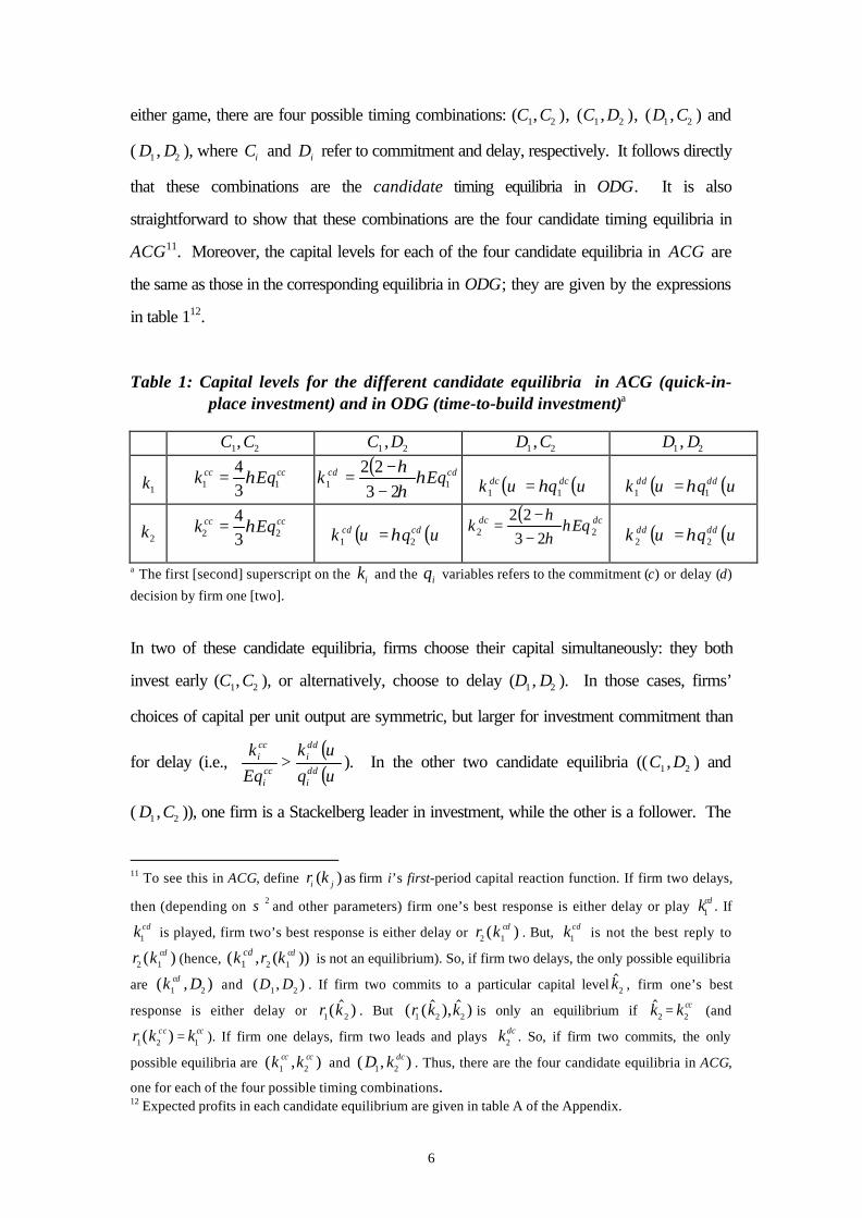
either game, there are four possible timing combinations: (C C1 2, ), (C D1 2, ), (D C1 2, ) and

( D D1 2, ), where Ci and Di refer to commitment and delay, respectively. It follows directly

that these combinations are the candidate timing equilibria in ODG. It is also

straightforward to show that these combinations are the four candidate timing equilibria in

ACG11. Moreover, the capital levels for each of the four candidate equilibria in ACG are

the same as those in the corresponding equilibria in ODG; they are given by the expressions

in table 112.

Table 1: Capital levels for the different candidate equilibria in ACG (quick-in-place investment) and in ODG (time-to-build investment)a

C C1 2, C D1 2, D C1 2, D D1 2,

k1k Eqcc cc

1 1

43

= η ( ) cdcd Eqk 11 2322 η

ηη

−−= ( ) ( )uquk dcdc

11 η= ( ) ( )uquk dddd11 η=

k2k Eqcc cc

2 2

43

= η ( ) ( )uquk cdcd21 η=

( ) dcdc Eqk 22 2322

ηηη

−−

= ( ) ( )uquk dddd22 η=

a The first [second] superscript on the ki and the qi variables refers to the commitment (c) or delay (d)

decision by firm one [two].

In two of these candidate equilibria, firms choose their capital simultaneously: they both

invest early (C C1 2, ), or alternatively, choose to delay (D D1 2, ). In those cases, firms’

choices of capital per unit output are symmetric, but larger for investment commitment than

for delay (i.e., ( )( )uq

uk

Eq

kddi

ddi

cci

cci > ). In the other two candidate equilibria ((C D1 2, ) and

( D C1 2, )), one firm is a Stackelberg leader in investment, while the other is a follower. The

11 To see this in ACG, define r ki j( ) as firm i’s first-period capital reaction function. If firm two delays,

then (depending on σ 2 and other parameters) firm one’s best response is either delay or play kcd1 . If

k cd1 is played, firm two’s best response is either delay or r k cd

2 1( ) . But, k cd1 is not the best reply to

r k cd2 1( ) (hence, ( , ( ))k r kcd cd

1 2 1 is not an equilibrium). So, if firm two delays, the only possible equilibria

are ( , )k Dcd1 2 and ( , )D D1 2 . If firm two commits to a particular capital level $k2 , firm one’s best

response is either delay or r k1 2( $ ) . But ( ( $ ), $ )r k k1 2 2 is only an equilibrium if $k2 = k cc2 (and

r k cc1 2( ) = k cc

1 ). If firm one delays, firm two leads and plays k dc2 . So, if firm two commits, the only

possible equilibria are ( , )k kcc cc1 2 and ( , )D k dc

1 2 . Thus, there are the four candidate equilibria in ACG,

one for each of the four possible timing combinations.12 Expected profits in each candidate equilibrium are given in table A of the Appendix.

7

committed capital level per unit output chosen by the leader is larger than that chosen by

either firm when both firms commit (k

EqkEq

kEq

cd

cd

dc

dcicc

icc

1

1

2

2

= > ).

In the next two sections, we derive and discuss the investment-timing pattern that emerges

with quick-in-place and time-to-build investment respectively, when firms have symmetric

costs ( 21 cc = and 21 AA = ). To prevent the discussion from becoming too taxonomical,

only pure strategies are considered. Since the analysis involves many unwieldy algebraic

expressions, graphical simulations are extensively used to ease the exposition. This

approach allows us to minimise the number of equations we give in the text, but does not

reduce the generality of our analysis in any way.

3. Quick-in-place investment

In this section we look at the benchmark game, ACG, which captures quick-in-place

investment in a simple and straightforward manner: if a firm decides to commit, it will do so

by choosing an investment level in stage one; however, if investment delay is preferred, the

firm chooses its capital investment flexibly in the second period (see figure 1a). Which of the

candidate equilibria represented in table 1, if any, eventually prevail, depends crucially on the

level of uncertainty (σ2 ) and the η-parameter (which is inversely related to the marginal

cost of capital) 13. This benchmark allows us to assess how strategic incentives change when

investment takes time to build.

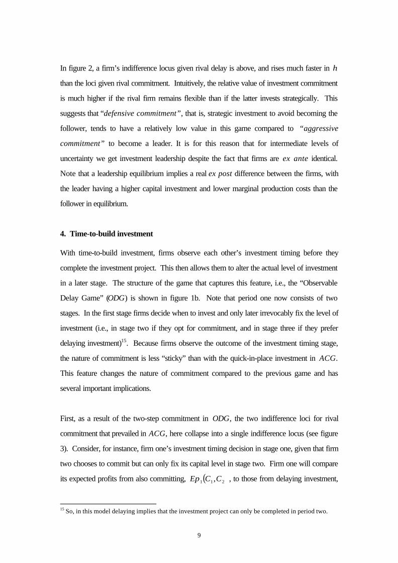
The investment timing that emerges is shown in ( ησ ,2 )-space (where σ σ2 212≡ / A is the

normalised variance) in figure 2. This figure gives loci along which a firm is indifferent

between commitment and delay, given a particular investment timing choice of its rival. At

levels of uncertainty (σ2 ) above the relevant locus, the firm prefers to delay, given the choice

made by its rival. At levels of uncertainty below the locus, it will commit. Along the top

locus ( ),(),( 211211 DDEDCE ππ = ), firm one is indifferent between commitment and

13 Throughout the paper the η-values are limited to guarantee interior solutions and by stabilityconsiderations.

8

delay, given that its rival delays its investment. Above this locus, the expected profit from

delay exceeds that from commitment (given rival delay). The lower two loci represent

commitment-delay indifference curves given rival commitment. When the rival commits in

ACG, it is committed to a particular investment level. Hence, to find the relevant

investment timing indifference curves we must take the actual investment level into account.

As mentioned earlier, there are two candidate equilibrium capital levels for firm two if it

commits, dck2 and cck 2 . There are therefore two relevant indifference curves given rival

commitment: one given that firm two commits to the leadership capital level, dck2

( ),(),( 211211dcdc kDEkCE ππ = ) and another one given that firm two chooses the capital

level prevailing under simultaneous commitment, cck 2 ( ),(),( 211211cccc kDEkCE ππ = ).

Thus, figure 3 depicts a total of three indifference curves for each firm. Given cost

symmetry, the loci of firm one naturally coincide with those of firm two. The difference

between these indifference curves as well as their implications for the equilibrium outcomes

are discussed in Appendix B.

[Figure 2 about here]

In figure 2, the ( ησ ,2 )-space is divided into four areas by the firms’ indifference loci. In

area IV, both firms delay investment. In this region the level of uncertainty is too high for

firms to forego flexibility. Delaying investment is preferred by each firm, independently of

the rival’s timing choice, hence delay by both is the unique equilibrium. In area III, there are

two leader-follower equilibria. Here, each firm prefers to delay if its rival commits. On the

other hand, if a firm’s rival delays, commitment will be chosen. Only in region I is uncertainty

so low that commitment by both firms, the outcome that would prevail under certainty, is the

unique equilibrium. Finally, in region II, the two leadership equilibria and commitment by

both firms are sustained as equilibria. Note, however, that this region is very narrow,

especially at low values of η 14. One could argue that region II is merely a fuzzy boundary

between areas I and III, caused by the inherent stickiness of early investment in ACG.

14 For instance, at η= 015. , region II is only 0.00060 wide in terms of σ 2 , while this distance narrows

down even further to a 2σ -range of 0.00005 at η= 0 05. .

9

In figure 2, a firm’s indifference locus given rival delay is above, and rises much faster in η

than the loci given rival commitment. Intuitively, the relative value of investment commitment

is much higher if the rival firm remains flexible than if the latter invests strategically. This

suggests that “defensive commitment”, that is, strategic investment to avoid becoming the

follower, tends to have a relatively low value in this game compared to “aggressive

commitment” to become a leader. It is for this reason that for intermediate levels of

uncertainty we get investment leadership despite the fact that firms are ex ante identical.

Note that a leadership equilibrium implies a real ex post difference between the firms, with

the leader having a higher capital investment and lower marginal production costs than the

follower in equilibrium.

4. Time-to-build investment

With time-to-build investment, firms observe each other’s investment timing before they

complete the investment project. This then allows them to alter the actual level of investment

in a later stage. The structure of the game that captures this feature, i.e., the “Observable

Delay Game” (ODG) is shown in figure 1b. Note that period one now consists of two

stages. In the first stage firms decide when to invest and only later irrevocably fix the level of

investment (i.e., in stage two if they opt for commitment, and in stage three if they prefer

delaying investment)15. Because firms observe the outcome of the investment timing stage,

the nature of commitment is less “sticky” than with the quick-in-place investment in ACG.

This feature changes the nature of commitment compared to the previous game and has

several important implications.

First, as a result of the two-step commitment in ODG, the two indifference loci for rival

commitment that prevailed in ACG, here collapse into a single indifference locus (see figure

3). Consider, for instance, firm one’s investment timing decision in stage one, given that firm

two chooses to commit but can only fix its capital level in stage two. Firm one will compare

its expected profits from also committing, ( )211 ,CCEπ , to those from delaying investment,

15 So, in this model delaying implies that the investment project can only be completed in period two.

10

( )211 ,CDEπ , knowing that its investment timing choice will affect the optimal level of firm

two’s capital in stage two ( k cc2 if C1 and k dc

2 if D1 ). Because firms now have to take into

account the effect of their own investment timing decision on the rival’s capital level, there is

only one indifference locus given rival commitment, implying that each firm now only has two

indifference loci in total.

Second, by contrast to the game with quick-in-place investment, the indifference locus for a

particular firm given rival commitment is above and steeper than its corresponding locus

given rival delay. This suggests that in ODG firms tend to invest early more for defensive

than for aggressive reasons, that is, more out of fear of ending up as the follower than to gain

a first-mover advantage. In ACG, the opposite was true; there, “aggressive commitment”

was more valuable than “defensive commitment”.

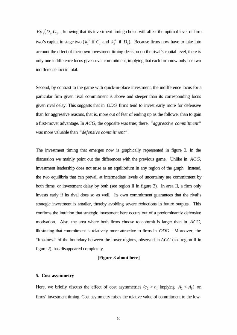
The investment timing that emerges now is graphically represented in figure 3. In the

discussion we mainly point out the differences with the previous game. Unlike in ACG,

investment leadership does not arise as an equilibrium in any region of the graph. Instead,

the two equilibria that can prevail at intermediate levels of uncertainty are commitment by

both firms, or investment delay by both (see region II in figure 3). In area II, a firm only

invests early if its rival does so as well. Its own commitment guarantees that the rival’s

strategic investment is smaller, thereby avoiding severe reductions in future outputs. This

confirms the intuition that strategic investment here occurs out of a predominantly defensive

motivation. Also, the area where both firms choose to commit is larger than in ACG,

illustrating that commitment is relatively more attractive to firms in ODG. Moreover, the

“fuzziness” of the boundary between the lower regions, observed in ACG (see region II in

figure 2), has disappeared completely.

[Figure 3 about here]

5. Cost asymmetry

Here, we briefly discuss the effect of cost asymmetries ( 12 cc > implying 12 AA < ) on

firms’ investment timing. Cost asymmetry raises the relative value of commitment to the low-

11

cost firm. Hence, each indifference locus of the latter will lie above the corresponding

indifference locus of its high-cost rival.

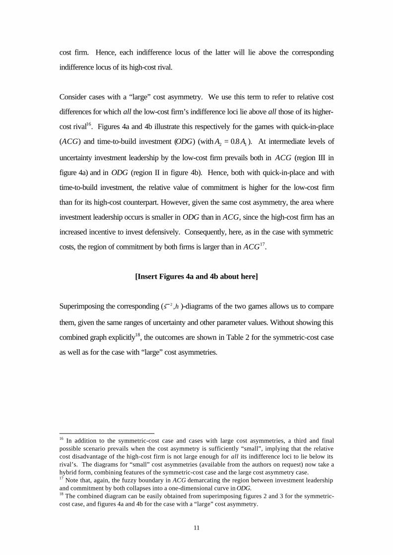
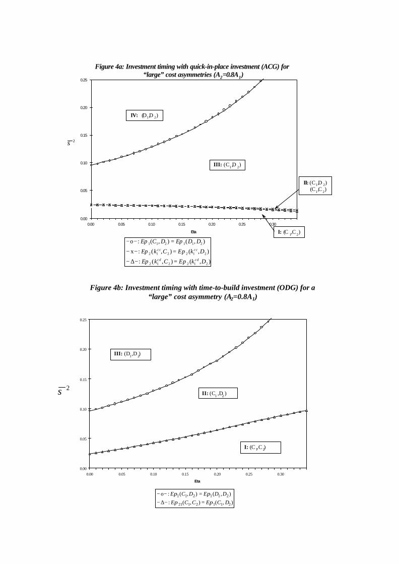
Consider cases with a “large” cost asymmetry. We use this term to refer to relative cost

differences for which all the low-cost firm’s indifference loci lie above all those of its higher-

cost rival16. Figures 4a and 4b illustrate this respectively for the games with quick-in-place

(ACG) and time-to-build investment (ODG) (with A A2 108= . ). At intermediate levels of

uncertainty investment leadership by the low-cost firm prevails both in ACG (region III in

figure 4a) and in ODG (region II in figure 4b). Hence, both with quick-in-place and with

time-to-build investment, the relative value of commitment is higher for the low-cost firm

than for its high-cost counterpart. However, given the same cost asymmetry, the area where

investment leadership occurs is smaller in ODG than in ACG, since the high-cost firm has an

increased incentive to invest defensively. Consequently, here, as in the case with symmetric

costs, the region of commitment by both firms is larger than in ACG17.

[Insert Figures 4a and 4b about here]

Superimposing the corresponding ( ησ ,2 )-diagrams of the two games allows us to compare

them, given the same ranges of uncertainty and other parameter values. Without showing this

combined graph explicitly18, the outcomes are shown in Table 2 for the symmetric-cost case

as well as for the case with “large” cost asymmetries.

16 In addition to the symmetric-cost case and cases with large cost asymmetries, a third and finalpossible scenario prevails when the cost asymmetry is sufficiently “small”, implying that the relativecost disadvantage of the high-cost firm is not large enough for all its indifference loci to lie below itsrival’s. The diagrams for “small” cost asymmetries (available from the authors on request) now take ahybrid form, combining features of the symmetric-cost case and the large cost asymmetry case.17 Note that, again, the fuzzy boundary in ACG demarcating the region between investment leadershipand commitment by both collapses into a one-dimensional curve in ODG.18 The combined diagram can be easily obtained from superimposing figures 2 and 3 for the symmetric-cost case, and figures 4a and 4b for the case with a “large” cost asymmetry.

12

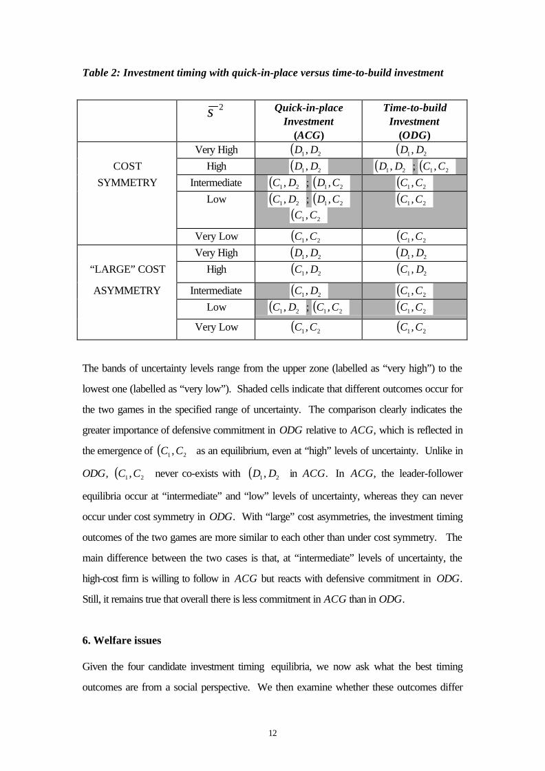
Table 2: Investment timing with quick-in-place versus time-to-build investment

σ 2 Quick-in-placeInvestment

(ACG)

Time-to-buildInvestment

(ODG)Very High ( )21 , DD ( )21 , DD

COST High ( )21 , DD ( )21 , DD ; ( )21 ,CC

SYMMETRY Intermediate ( )21 , DC ; ( )21 ,CD ( )21 ,CC

Low ( )21 , DC ; ( )21 ,CD( )21 ,CC

( )21 ,CC

Very Low ( )21 ,CC ( )21 ,CC

Very High ( )21 , DD ( )21 , DD

“LARGE” COST High ( )21 , DC ( )21 , DC

ASYMMETRY Intermediate ( )21 , DC ( )21 ,CC

Low ( )21 , DC ; ( )21 ,CC ( )21 ,CC

Very Low ( )21 ,CC ( )21 ,CC

The bands of uncertainty levels range from the upper zone (labelled as “very high”) to the

lowest one (labelled as “very low”). Shaded cells indicate that different outcomes occur for

the two games in the specified range of uncertainty. The comparison clearly indicates the

greater importance of defensive commitment in ODG relative to ACG, which is reflected in

the emergence of ( )21 ,CC as an equilibrium, even at “high” levels of uncertainty. Unlike in

ODG, ( )21 ,CC never co-exists with ( )21 , DD in ACG. In ACG, the leader-follower

equilibria occur at “intermediate” and “low” levels of uncertainty, whereas they can never

occur under cost symmetry in ODG. With “large” cost asymmetries, the investment timing

outcomes of the two games are more similar to each other than under cost symmetry. The

main difference between the two cases is that, at “intermediate” levels of uncertainty, the

high-cost firm is willing to follow in ACG but reacts with defensive commitment in ODG.

Still, it remains true that overall there is less commitment in ACG than in ODG.

6. Welfare issues

Given the four candidate investment timing equilibria, we now ask what the best timing

outcomes are from a social perspective. We then examine whether these outcomes differ

13

from those generated by the market with time-to-build and with quick-in-place investment.

In our partial equilibrium set-up, welfare is naturally defined as the sum of expected

consumer surplus and expected industry profits19. Capital commitment implies strategic

behaviour with investment above the cost minimising level. From a social perspective, more

capital commitment therefore raises the social cost of investment and, in addition, foregoes

the social benefits from flexibility. However, it will also lead to higher production and

therefore lower prices for consumers.

In figures 5a and 5b, the actual investment-timing outcomes (with cost symmetry) are

indicated by superscript m, while the socially preferred outcomes are superscripted by s. A

shaded label highlights the areas in which the market outcome differs from the socially

preferred investment timing. For both games the socially preferred timing outcomes coincide

with the market outcomes at fairly high (area IV in figures 5a and 5b) and at fairly low (area

I) uncertainty. In the former case, both firms delay, whereas they both commit in the latter

case. At moderate levels of uncertainty (areas II and III), however, comparing the socially

preferred outcomes to the ones generated by the market leads to different implications in

ACG than in ODG. In ACG (figure 5a), the market produces too much commitment in area

III, but too little commitment in area IIb (and possibly in area IIa). In ODG (figure 5b), the

market will never produce too little but may involve too much strategic commitment (i.e., the

market generates ( 21 ,CC ) where ( 21, DD ) is socially preferred)20.

[Insert Figures 5a and 5b about here]

This brief positive welfare analysis indicated which of the four candidate investment timing

equilibria yield the highest welfare for different ranges of uncertainty and allowed us to

compare these with those generated by the market. However, it is clear that policy

intervention could improve welfare since the oligopoly distortion implies that firms are

producing too little. In addition, when firms are investing strategically they choose more than

19 Like profits, consumer surplus is convex in u, implying that consumers also like firms to be flexible.20 When there is a substantial cost asymmetry between firms, we find that comparisons between themarket and the socially preferred outcomes are qualitatively the same for both games. Having the low-cost firm as the leader is socially preferred unless uncertainty is very high.

14

the socially cost-minimising capital level21. The standard instruments to deal with these

distortions are production subsidies and capital taxes. Moreover, besides affecting the

levels of output and investment, the government may also wish to change firms’ investment

timing. Compared to quick-in-place investment, more firms tend to invest too early with

time-to-build investment. As a result they lose their flexibility, implying that the government

may want to engage in commitment deterrence22. Hence, a first-best package of policies will

simultaneously and directly address these three possible inefficiencies of underproduction,

overinvestment and inflexibility.

7. Conclusion

The implications of the simple real-world fact that investment projects take time to complete

were considered in an oligopoly setting. Standard investment theory finds that an increase in

uncertainty causes delay. However, under oligopoly with quantity-setting firms, there is an

incentive to invest early. There are two closely related reasons for this. First, there is an

aggressive motive to win a first-mover advantage and second, there is a defensive motive to

avoid being saddled with a second-mover disadvantage. We have shown that a time lag

between when and how much to invest reduces the incentive to delay induced by

uncertainty. In particular, the defensive motive for early investment is greater when

investment requires time to put in place. We have shown that with such investment projects,

firms within the industry all tend to invest early at levels of uncertainty for which some firms

would have delayed if the investment were of the quick-in-place type. This is consistent

with Bar-Ilan and Strange (1996), who find –in a totally different model without strategic

behaviour- that time-to-build induces firms to invest earlier rather than later.

A case study of the bulk chemical industry by Ghemawat (1984) provides empirical

confirmation of our model’s predictions. Two of his observations are particularly relevant

here. First, he concluded that the lowest-cost producer in the titanium dioxide industry, Du

Pont, chose for investment leadership as a deliberate growth strategy. This corroborates

21 This distortion is absent in models that are concerned with endogenous production -as distinct frominvestment- timing. Hence, a welfare analysis (of which, to our knowledge, there are as yet no examples)in such models would differ from ours.22 Dewit and Leahy (2001) consider policies to deter commitment in an open economy setting.

15

our finding that, in the presence of cost asymmetries, the low-cost firm has the greater

incentive to invest early. Second, he points out how the presence of significant construction

lags in the industry effectively allowed “defensive” commitment. He cites (p. 157) how one

firm, Kerr-McGee, prevented its rival, Du Pont, from obtaining a first-mover advantage: by

introducing its own investment plans before Du Pont’s expansion had fully materialised,

Kerr-McGee forced Du Pont to revise its initial capacity plans. This illustrates the difficulty

of effectively obtaining leadership with time-to-build investment, as was emphasised in our

paper.

Finally, our paper explored the welfare implications of time-to-build investment. Our

analysis suggests that in industries in which investment takes time to be completed firms tend

to invest too early from a social perspective. Too much investment delay, however, never

occurs. This is not true with quick-in-place investment; then, even at moderate levels of

uncertainty, it is possible that not enough firms invest early. These findings suggest that

investment policies may require a lot more thought and may possibly need to take into

account the duration of investment projects until completion.

16

Appendix A

Table A: Expected profits in the different candidate equilibria under ActionCommitment and Observable Delay

21 ,CC 21 , DC 21 ,CD 21, DD

1πE ( ) 22

1 91

σγ +ccEq ( ) 2

22

1 231

ση

ηζ

−−

+cdEq ( )( )

22

2

123

2/1σ

ηη

ϕ−−

+dcEq ( ) ( )( )

22

2

13

2/1σ

ηη

ϕ−

−+ddEq

2πE ( ) 22

2 91

σγ +ccEq ( )( )

22

2

223

2/1σ

ηη

ϕ−−

+cdEq ( ) 2

22

2 231

ση

ηζ

−−

+dcEq ( ) ( )( )

22

2

2 3

2/1σ

ηη

ϕ−

−+ddEq

with ( )ηγ 9/81 −≡ , 2

232

21

−−−≡

ηηηζ and 2/1 ηϕ −≡ .

Appendix B: Determination of the investment timing equilibria

(i) The investment timing equilibria with quick-in-place investment (ACG)

To find the equilibria in different regions of the ( ησ ,2 )-space we proceed by asking when

each of the candidate equilibria will not be an equilibrium. For concreteness and without

loss of generality, we consider possible deviations by firm one from each candidate

equilibrium.

(a) The candidate equilibrium ( )21 , DD

On the highest locus in figure 2, each firm is indifferent between commitment and delay given

investment delay by its rival. Given rival delay, firm one, in deciding when to invest,

compares the profits ( )211 , DDEπ and ( )211 , DCEπ , taking into account that its rival

reacts to its investment timing decision. For instance, on the locus

( ( ) ( )211211 ,, DDEDCE ππ = ) firm one is indifferent between choosing k cd1 in period one

and delaying its capital choice until period two (when it will choose k udd1 ( ) ). Below this

locus (areas I-III), ( , )D D1 2 cannot be an equilibrium.

(b) The candidate equilibria ),( 21 DC and ),( 21 CD

The highest locus in figure 2 also demarcates the maximum uncertainty upper limit for the

leader-follower equilibria, ( , )C D1 2 = ( , )k Dcd1 2 and ( , )D C1 2 = ( , )D k dc

1 2 . In other words,

( , )C D1 2 (and by symmetry ( , )D C1 2 ) cannot be an equilibrium above this locus (area IV),

since in that region ( ) ( )211211 ,, DDEDkE cd ππ < . The lowest of the three loci in the figure

provides the lower bound for leader-follower equilibria. Below this locus (area I) we have

17

( ) ( )dcdc kDEkCE 211211 ,, ππ > , and hence firm one will wish to deviate from delay given that

firm two chooses the investment leadership capital level, k dc2 .

(c) The candidate equilibrium ( , )C C1 2

This is an equilibrium at 02 =σ , when there are no flexibility advantages of delaying and

both firms commit, regardless of the timing strategy of their rival. Next, consider the range of

σ2 and η over which ( , )C C1 2 =( , )k kcc cc1 2 cannot be an equilibrium. Given k cc

2 , there is a

locus (the second highest in figure 2) along which firm one is indifferent between commitment

and delay. Above this locus (areas III and IV), we have ( ) ( )cccc kDEkCE 211211 ,, ππ < ,

hence, firm one wants to delay and therefore ( , )C C1 2 cannot be an equilibrium. On or

below the locus, firm one will not wish to deviate from k cc1 (by symmetry, firm two will not

want to deviate from k cc2 in that region). Thus, commitment by both firms will be an

equilibrium at all uncertainty levels that are not above this locus.

(ii) The investment timing equilibria with time-to-build investment (ODG)

The investment timing equilibria are determined by a method similar to the one described in

(i), but now using the loci represented in figure 3.

(a) The candidate equilibria ( 21, DD ) and ( 21 ,CC )

Above both indifference loci in figure 3 (area III) delay will be played by each firm,

regardless of its rival’s timing choice. Hence, ( 21, DD ) is the unique equilibrium in area III.

Below both indifference loci (area I), commitment will be played by each firm, regardless of

its rival’s timing choice. Hence, ( 21 ,CC ) is the unique equilibrium in area I. In the

intermediate region (area II), commitment is the best response to rival commitment, while

delay is the best response to rival delay. Therefore, both ( 21, DD ) and ( 21 ,CC ) are

equilibria in area II.

(b) The candidate equilibria ( 21 ,DC ) and ( 21 ,CD )

When commitment is the best response to delay (area I), delay is not the best response to

commitment, but, when delay is the best response to commitment (area III), commitment is

not the best response to delay. Hence, ( 21 ,DC ) and ( 21 ,CD ) are never equilibria.

18

References

Appelbaum, E. and C. Lim (1985), “Contestable markets under uncertainty”, RandJournal of Economics, 16, 28-40.

Bar-Ilan, A. and W. Strange (1996), “Investment lags”, American Economic Review, 86,610-622.

Boyer, M and M. Moreaux (1997), “Capacity commitment versus flexibility”, Journal ofEconomics and Management Strategy, 1, 347-376.

Canoy, M. and P. Van Cayseele (1996), “Endogenous price leadership with a front-runner”, Centre for Economic Studies, KU Leuven, Discussion Paper Series,Financial Economics Research Paper No. 26.

Dewit, G. and D. Leahy (2001), “Rivalry in Uncertain Export Markets: Commitmentversus Flexibility”, Economics Department Working Papers Series,N105/02/01, National University of Ireland, Maynooth.

Dixit, A. and R. Pindyck (1994), Investment under uncertainty. New Jersey: PrincetonUniversity Press.

Ghemawat, P. (1984), “Capacity expansion in the titanium dioxide industry”, Journal ofIndustrial Economics, 33, 145-163.

Grossman, G. and G. Maggi (1998), “Free trade vs. strategic trade: A peek into Pandora’sBox”, in R. Sato, R.V. Ramachandran, and K. Mino (eds.): Global Integrationand Competition, Kluwer Academic Publishers, Dordrecht, 9-32.

Hamilton, J. and S. Slutsky (1990), “Endogenous timing in duopoly games Stackelberg orCournot equilibria”, Games and Economic Behavior, 2, 29-46.

Kydland, F. and E. Prescott (1982), “Time to build and aggregate fluctuations”,Econometrica, 50, 1345-1370.

Majd, S. and R. Pindyck (1987), “Time to build, option value and investment decisions”,Journal of Financial Economics, 1987, 18, 7-27.

Pal, D. (1996), “Endogenous Stackelberg equilibria with identical firms”, Games andEconomic Behavior, 12, 81-94.

Pindyck, R. (1991), “Irreversibility, uncertainty, and investment”, Journal of EconomicLiterature, 29, 1110-1148.

Sadanand, A. and V. Sadanand (1996), “Firm scale and endogenous timing of entry: achoice between commitment and flexibility”, Journal of Economic Theory, 70,516-530.

Spencer, B. and J. Brander (1992), “Pre-commitment and flexibility: Applications tooligopoly theory”, European Economic Review, 36, 1601-1626.

Tirole, J. (1988), The Theory of Industrial Organization, Cambridge, Massachusetts: TheMIT Press.

Vives, X. (1989), “Technological competition, uncertainty, and oligopoly”, Journal ofEconomic Theory, 48, 386-415.

C C1 2,

C D1 2,

D C1 2,

D D1 2,

k kcc cc1 2,

k cd1 ,−

−, k dc2

− −,

q q1 2,

q k qcd1 2 2, ,

k q qdc1 1 2, ,

k q k qdd dd1 1 2 2, , ,

Stage 1Timingchoices

Stage 2Committed

capitalchoices

Stage 3Flexible capital

and outputchoices

t=1Uncertainty

t=2Certainty

Figure 1b: The game with time-to-build investment (ODG)

k kcc cc1 2,

k Dcd1 2,

D k dc1 2,

D D1 2,

q q1 2,

q k qcd1 2 2, ,

k q qdc1 1 2, ,

k q k qdd dd1 1 2 2, , ,

Stage 1Timing and

committed capitalchoices

Stage 2Flexible capital

and outputchoices

t=1Uncertainty

t=2Certainty

Figure 1a: The game with quick-in-place investment (ACG)

0.00

0.05

0.10

0.15

0.20

0.25

0.00 0.05 0.10 0.15 0.20 0.25 0.30 0.35Eta

σ2

IV: (D1,D2)

I: (C1,C2)

III: (C1,D2) (D1, C2)

(C1,D2)II: (D1, C2) (C1,C2)

),(),( and ),(),(:

),(),( and ),(),(:x

),(),( and ),(),(:o

212212211211

212212211211

212212211211

DkECkEkDEkCE

DkECkEkDEkCE

DDECDEDDEDCE

cdcddcdc

cccccccc

ππππ

ππππ

ππππ

==−∆−

==−−

==−−

Figure 2: Investment timing with quick-in-place investment (ACG) forcost symmetry (A1=A2)

0.00

0.05

0.10

0.15

0.20

0.25

0.00 0.05 0.10 0.15 0.20 0.25 0.30 0.35

Eta

σ2

III: (D1,D2)

I: (C1,C2)

II: (D1,D2); (C1 ,C2)

),(),( and ),(),(:o

),(),( and ),(),(:

212212211211

212212211211

DDECDEDDEDCE

DCECCECDECCE

ππππππππ

==−−==−∆−

Figure 3: Investment timing with time-to-build investment (ODG) forcost symmetry (A1=A2 )

0.00

0.05

0.10

0.15

0.20

0.25

0.00 0.05 0.10 0.15 0.20 0.25 0.30

Eta

IV: (D1,D 2)

III: (C1,D 2)

I: (C 1,C 2)

II: (C1,D 2) (C1,C 2)

σ 2

),(),(:

),(),(:x

),(),(:o

212212

212212

211211

DkECkE

DkECkE

DDEDCE

cdcd

c cc c

ππ

ππ

ππ

=−∆−

=−−

=−−

Figure 4a: Investment timing with quick-in-place investment (ACG) for“large” cost asymmetries (A2=0.8A1)

σ 2

Figure 4b: Investment timing with time-to-build investment (ODG) for a“large” cost asymmetry (A2=0.8A1)

0.00

0.05

0.10

0.15

0.20

0.25

0.00 0.05 0.10 0.15 0.20 0.25 0.30

Eta

),(),(:

),(),(:o

2112121

211211

DCECCE

DDEDCE

ππππ

=−∆−=−−

III: (D1,D 2)

II: (C1 ,D2 )

I: (C 1,C 2)

(C 1,D2)m

(D1, C2)m

(C1,C2)m

(C1,C2)s

(C1,D2) (D1, C2)

(C1,C2)s

Figure 5a: Market outcomes versus socially preferred outcomes with quick-in-place investment (ACG) for cost symmetry (A1=A2)

σ2

),(),(:*

),(),( and ),(),(:

),(),( and ),(),(:x

),(),( and ),(),(:o

2121

212212211211

212212211211

212212211211

DDEWCCEW

DkECkEkDEkCE

DkECkEkDEkCE

DDECDEDDEDCE

cdcddcdc

cccccccc

=−−==−∆−

==−−

==−−

ππππ

ππππ

ππππ

0.00

0.02

0.04

0.06

0.08

0.10

0.12

0.14

0.16

0.18

0.20

0.00 0.05 0.10 0.15 0.20 0.25 0.30 0.35

Eta

(D1,D2)m

(D1,D2)s

(C1,D2)m

(D1, C2)m

(D1,D2)s

(C1,C2)m

(C1,C2)s

0.00

0.02

0.04

0.06

0.08

0.10

0.12

0.14

0.16

0.18

0.20

0.00 0.05 0.10 0.15 0.20 0.25 0.30 0.35

Eta

2σ

(D1,D2)m

(D1,D2)s

(D1,D2)m ; (C1,C2)m

(D1,D2)s

(C1,C

2)m

(D1,D2)s

(C1,C2)m(C1,C2)s

),(),(:*

),(),( and ),(),(:o

),(),( and ),(),(:

2121

212212211211

212212211211

DDE WCCE W

DDECDEDDEDCE

DCECCECDECCE

=−−==−−

==−∆−

ππππ

ππππ

Figure 5b: Market outcomes versus socially preferred outcomes with time-to-build investment (ODG) for cost symmetry (A1=A2)