CENTER PIVOT DESIGN AND EVALUATION
14
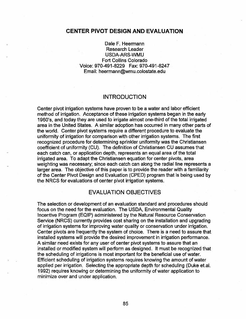
CENTER PIVOT DESIGN AND EVALUATION Dale F. Heermann Research Leader USDA-ARS-WMU Fort Collins Colorado Voice: 970-491-8229 Fax: 970-491-8247 Email: [email protected] INTRODUCTION Center pivot irrigation systems have proven to be a water and labor efficient method of irrigation. Acceptance of these irrigation systems began in the early 1960's, and today they are used to irrigate almost one-third of the total irrigated area in the United States. A similar adoption has occurred in many other parts of the world. Center pivot systems require a different procedure to evaluate the uniformity of irrigation for comparison with other irrigation systems. The first recognized procedure for determining sprinkler uniformity was the Christiansen coefficient of uniformity (CU). The definition of Christiansen CU assumes that each catch can, or application depth, represents an equal area of the total irrigated area. To adapt the Christiansen equation for center pivots, area weighting was necessary; since each catch can along the radial line represents a larger area. The objective of this paper is to provide the reader with a familiarity of the Center Pivot Design and Evaluation (CPED) program that is being used by the NRCS for evaluations of center pivot irrigation systems. EVALUATION OBJECTIVES The selection or development of an evaluation standard and procedures should focus on the need for the evaluation. The USDA, Environmental Quality Incentive Program (EQIP) administered by the Natural Resource Conservation Service (NRCS) currently provides cost sharing on the installation and upgrading of irrigation systems for improving water quality or conservation under irrigation. Center pivots are frequently the system of choice. There is a need to assure that installed systems will provide the desired improvement in irrigation performance. A similar need exists for any user of center pivot systems to assure that an installed or modified system will perform as designed. It must be recognized that the scheduling of irrigations is most important for the beneficial use of water. Efficient scheduling of irrigation systems requires knowing the amount of water applied per irrigation. Selecting the appropriate depth for scheduling (Duke et.al. 1992) requires knowing or determining the uniformity of water application to minimize over and under application. 85
Transcript of CENTER PIVOT DESIGN AND EVALUATION
CENTER PIVOT DESIGN AND EVALUATION
Dale F. Heermann Research Leader USDA-ARS-WMU
Fort Collins Colorado Voice: 970-491-8229 Fax: 970-491-8247
Email: [email protected]
INTRODUCTION
Center pivot irrigation systems have proven to be a water and labor efficient method of irrigation. Acceptance of these irrigation systems began in the early 1960's, and today they are used to irrigate almost one-third of the total irrigated area in the United States. A similar adoption has occurred in many other parts of the world. Center pivot systems require a different procedure to evaluate the uniformity of irrigation for comparison with other irrigation systems. The first recognized procedure for determining sprinkler uniformity was the Christiansen coefficient of uniformity (CU). The definition of Christiansen CU assumes that each catch can, or application depth, represents an equal area of the total irrigated area. To adapt the Christiansen equation for center pivots, area weighting was necessary; since each catch can along the radial line represents a larger area. The objective of this paper is to provide the reader with a familiarity of the Center Pivot Design and Evaluation (CPED) program that is being used by the NRCS for evaluations of center pivot irrigation systems.
EVALUATION OBJECTIVES
The selection or development of an evaluation standard and procedures should focus on the need for the evaluation. The USDA, Environmental Quality Incentive Program (EQIP) administered by the Natural Resource Conservation Service (NRCS) currently provides cost sharing on the installation and upgrading of irrigation systems for improving water quality or conservation under irrigation. Center pivots are frequently the system of choice. There is a need to assure that installed systems will provide the desired improvement in irrigation performance. A similar need exists for any user of center pivot systems to assure that an installed or modified system will perform as designed. It must be recognized that the scheduling of irrigations is most important for the beneficial use of water. Efficient scheduling of irrigation systems requires knowing the amount of water applied per irrigation. Selecting the appropriate depth for scheduling (Duke et.al. 1992) requires knowing or determining the uniformity of water application to minimize over and under application.
85
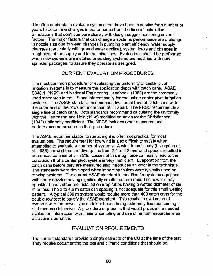
It is often desirable to evaluate systems that have been in service for a number of years to determine changes in performance from the time of installation. Simulations that don't compare closely with design suggest exploring several factors. The major factors that can change a systems performance are a change in nozzle size due to wear, changes in pumping plant efficiency, water supply changes (particularly with ground water decline), system leaks and changes in roughness of the supply and lateral pipe lines. Evaluations should be performed when new systems are installed or existing systems are modified with new sprinkler packages, to assure they operate as designed.
CURRENT EVALUATION PROCEDURES
The most common procedure for evaluating the uniformity of center pivot irrigation systems is to measure the application depth with catch cans. ASAE S346.1, (1999) and National Engineering Handbook, (1983) are the commonly used standards in the US and internationally for evaluating center pivot irrigation systems. The ASAE standard recommends two radial lines of catch cans with the outer end of the rows not more than 50 m apart. The NRSC recommends a single line of catch cans. Both standards recommend calculating the uniformity with the Heermann and Hein (1968) modified equation for the Christiansen (1942) uniformity coefficient. The NRCS includes other measures and performance parameters in their procedure.
The ASAE recommendation to run at night is often not practical for most evaluations. The requirement for low wind is also difficult to satisfy when attempting to evaluate a number of systems. A wind tunnel study (Livingston et. al. 1985) showed that the divergence from 2.5 to 6.2 mis wind speeds resulted in decreased catches of 5 - 25%. Losses of this magnitude can easily lead to the conclusion that a center pivot system is very inefficient. Evaporation from the catch cans before they are measured also introduces an error in the technique. The standards were developed when impact sprinklers were typically used on moving systems. The current ASAE standard is modified for systems equipped with spray nozzles having significantly smaller pattern radii. The newer spray sprinkler heads often are installed on drop tubes having a wetted diameter of six m or less. The 3 to 4.6 m catch can spacing is not adequate for this small wetting pattern. A typical 380 m system would require more than 400 catch cans for the double row test to satisfy the ASAE standard. This results in evaluation of systems with the newer type sprinkler heads being extremely time consuming and resource intensive. A procedure or process that would provide the needed evaluation information with minimal sampling and use of human resources is an attractive alternative.
EVALUATION REQUIREMENTS
The current standards provide a single estimate of the CU at the time of the test. They require documenting the test and climatic conditions that should be
86

鴯
considered when comparing tests between systems. The test however does not provide an insight to the performance of the system as it moves around the circle that is irrigated. The effect of topography and water supply characteristics should also be evaluated. It is a reasonable requirement to suggest that the tests be run under low wind speeds and low evaporation conditions. The NRCS spacing of 9.2 m maximum and ASAE standard 3m could result in errors with smaller radius sprinkler patterns.
ALTERNATIVE EVALUATION PROCEDURE
Computer simulation of the center pivot sprinkler performance was first presented by Heermann and Hein (1968). A user friendly simulation program Center Pivot Evaluation and Design (CPED) is currently being used by the NRCS evaluating center pivot systems. The required inputs and options for the model were presented by Heermann (1990). Edling (1979), James (1984), and Bremond and Molle (1995) have written simulation programs for evaluating different characteristics of center pivot systems. The distinct advantage of simulation over field tests is the large number of design options and operating conditions that can be compared with limited time and resources.
Suggested ProtocolforAIternative Procedure
Manufacturers and distributors of center pivot and/or sprinkler heads use computer models to design the vast majority of new or renozzled center pivot systems. Most system designs will provide a uniform irrigation if nozzles and sprinklers are installed according to the design and operated within their intended flow and pressure. The inventory of the manufacturer's computer design provides the majority of the inputs needed to run a simulation of the system to obtain the potential _uniformity of the system.
The next step would be to go to the field and perform a physical and visual inventory of the system. The size and length of all pipes, sprinkler model, nozzle sizes, pressure regulators, and location of each outlet should be compared with the design chart and inventory. The elevation of the pivot and each tower is needed for input to the simulation model to accurately solve for the pressure distribution on the system. It is desirable to use pump and drawdown curves but it can be run with constant pressure or discharge. An approximation of the pipe roughness is needed before running the simulation. With the system operating, pressure and discharge measurements should be taken along the lateral line and compared with the calculated pressures and discharges.
Model output includes the hydraulic operating pressures on the system, the sprinkler discharge, the application depth at requested positions and the coefficients of uniformity (Christiansen and low quarter). Differences between measured and computed pressures and discharges suggest that the system may not be performing as desired.
87
Potential causes of simulation errors are wear, age, or measurement errors of the components, which may cause the initial input to be in error. Factors that can change with age include the pipe roughness factor, pump curve, and nozzle size. Pressure regulators may have a hysteresis effect and could lead to differences between simulated and measured. Age also can change the performance of flow control devices. Measurement is always a potential source of error. This could include measured pressures, discharges, distances and elevation, recognizing accuracy is ± 5% with most standard measuring devices for flow and pressure.
SIMULATION EVALUATION OF CENTER PIVOT SYSTEMS
The simulation model in this paper is based on the first model presented by Heermann and Hein (1968) which was verified with field data. Their simulation model required input of the sprinkler location, discharge, pattern radius and an assumed stationary pattern shape of either triangular or elliptical. The application depth versus distance along a radial line from the pivot was determined and application rates at a specified distance from the pivot were determined. The hours per revolution were input and each tower was assumed to move at a constant speed for the complete circle. Kincaid, Heermann and Kruse (1969) used the model to calculate potential runoff for different system capacities and infiltration rates. Kincaid and Heermann (1970) added the calculation of the flow resistance and verified with measured pressure distribution along the center pivot lateral. Chu and Moe (1972) studied the hydraulics of a center pivot system and developed a quick approximation for determining the pressure loss from the pivot to the outer end of the lateral as a constant (0.543) times the loss that would occur if the entire discharge flowed the total length of the lateral.
The model was adapted by Beccard and Heermann (1981) to include the effect of topographic differences in the resulting application depths along radii of the center pivot in the non level fields. The model included the pump and well characteristics and calculated the hydraulic equilibrium point as the system moved to different positions on a rough terrain. The model was exercised to determine the uniformity changes when converting from high pressure to low pressure on rough terrain. Edling (1979), and James (1984) also used simulation models to study the performance of center pivot systems on variable topography and with different pressures.
The current simulation model has been expanded to include donut shaped stationary patterns that can be used to represent many of the low pressure spray applicators.
88
.

EXAMPLE OF SIMULATION EVALUATION
The uniformity of application depths can be calculated by inventorying the sprinkler head models, nozzles sizes and distance from the pivot. The pump curve and drawdown, or pivot pressure, or discharge is also needed. Figure 1 illustrates a simulation as designed and the distribution if the sprinkler heads were reversed between 2 towers made at the time of installation. Note that the change reduced the CU by 3 percent.
'̀ Capacity 一 3785 LPM Irrigated Area - 64 HA Unlfonnlly 一 90.8Unifoonily 一 87.9
4020 .戶U1
暑 --··` ·、丶-,
``~'
。
。 100 200 300 400 500
Dis!Bnce - M
Figure 1 Typical center pivot as designed (CU= 90.8) and with 10 sprinkler heads incorrectly installed shown as a dashed line (CU= 87.9)
THE CENTER PIVOT SYSTEM FILE
The following sections will give more provide an overview of the type of information needed in CPED. It will provide information of the representation of the data and how it is used in the simulation model. The inventory of the system is needed for the simulation. We refer to this information as the Center Pivot System File - or for convenience - The System file. To create a System File have the following information on hand from the manufacturer's inventory:
1. The pump curve or alternatively a constant discharge or constant head with and estimate of discharge. (The pump will be discussed in greater detail later.)
2. The Total Dynamic Lift (ft.), if using a pump curve.
3. The length (ft.), inside diameters (in.), and the Darcy-Weisbach resistance coefficients for the pump to pivot pipe and the riser pipe.
89

4. The pipe diameters, starting distances and Darcy - Weisbach Coefficients for the sprinkler pipe.
5. The pivot pad elevation and the height above the soil surface where the pressure is specified(ft.) (Either the pivot height or the sprinkler height if drops are used.)
6. The number of towers, the tower locations (ft.), and the tower elevations (ft.) relative to the pivot pad elevation.
7. The booster pump increase (psi) and the number of sprinklers affected by the increased pressure (used with end guns).
8. The sprinkler brand and model # of each sprinkler on the system. (This will be discussed in much more detail later.)
9. Distance (ft.), range nozzle diameter (64th in.), spreader no-zzle diameter (64th in.) for each sprinkler on the system (enter range no-zzle for one no之le sprinklers).
10. The type of pressure control and whether or not there are part circle sprinklers
11. For each pressure controlled sprinkler: the maximum pressure {psi); or the fixed orifice diameter (64th in.).
12. The start and stop angles for each part circle sprinkler.
13. The right and/or left offset for each offset sprinkler.
Some of these items need further explanation:
THE PUMP
PumQ Curve
The Head vs Discharge graph for the pump on the system can be used to develop the regression equation that describes the pump.. The program has an option which will fit the pump curve, after it has been given points
90

from the graph. At least 4 points that span the operating range are needed, however 8-10 will give a better fit. The form of the equation for the pump curve 1s:
where:
Q=B。 +81H + B武
Q - discharge - gpm H - head/stage - psi B。 -intercept81 - linear slope coefficient on head 82 - quadratic slope coefficient on head
The number of stages for the pump also needs to be entered, as most pump curves from the manufacturer are for a single stage. However, if the pump curve comes from field measurements, set the number of stages equal to one.
Constant Head
Rather than using a pump curve, it is also possible to specify a system with constant head or constant discharge. To use a Constant Head enter:
Constant Head - psi Estimate of Discharge at that Head - gpm
Set the number of stages equal to one.
Constant Djscha~_ge
To use a Constant Discharge enter: Constant Discharge - gpm
Set the number of stages equal to one.
SPRINKLER BRAND AND MODEL NUMBER
For each sprinkler model on the system, regression coefficients which estimate the coefficient of discharge and the pattern radius, based on the nozzle size and the pressure, are needed. The information provided in the manufacturers'catalogs is used to develop the equations.
Discharge Coefficient
Cd = Q/(~(2gH) 112) where:
91

Cd - discharge coefficient Q - discharge, from catalog - cfs A - equivalent area of the nozzle orifice - ftA2 ; A = Pl*(DR2 + Ds2)/4 DR - range nozzle diameter - ft Ds - spreader nozzle diameter - ft g - gravitational constant - 32.2 ft/sec/sec H - sprinkler pressure, from catalog - ft
These units are chosen for calculation such that Cd is dimensionless and between.9 to 1 for most manufacturers. Enter the catalog information in a spreadsheet, and use it to convert to the appropriate units and calculate the discharge coefficients. Once the discharge coefficients are calculated for the various combinations of pressure and nozzle radius, the regression equation to predict Cd can be fit. If the spreadsheet won't do multiple regression, export a file containing Cd, 02, and H, and use a statistics package that will. The equation is:
where:
Pattern Radius
Cd= B。 +8102 + B2H
C~ - discharge coefficient D2 - equivalent nozzle radius - ft2: D2 = (Dl + Ds2)/4 H - sprinkler pressure - ft B。 -Intercept81 - Slope on 02 82 - Slope on H
An equation that can be used to predict pattern radius based on range nozzle diameter and pressure is developed in an analogous manner. That equation is:
R=B。 +81 (DR2H) + 82(0启H)2
where: R - Pattern radius - ft DR - Range nozzle diameter-ft H - Pressure - ft B。 -Intercept81 - Slope on D語H82 - Slope on (D是H)2
Enter the data consisting of the Pattern Radius, the Range Nozzle diameter, and the Head from the manufacturer's catalog into a spreadsheet. Use the spreadsheet to make the units conversions and
92

calcul~te_DlH and (D語H)2. Then export an ASCII file containing R, D启H,& (DlH)2, t , to use in a statistics package that will fit multiple regression.
This pair of equations needs to be developed for each sprinkler used in a simulation. They are used in the simulation program to calculate the discharge and the pattern radius of each sprinkler in order to get the depths. Also needed is its minimum operating pressure in psi. We provide a data base containing the sprinklers we have fit.
RELATIVE ELEVATIONS
The relative elevations of the pivot pad and the towers are used to determine the slope changes of the system, therefore actual elevations aren't needed. The pivot pad elevation needs to be arbitrarily set high enough so that none of the tower elevations are negative. The tower elevations then are set so that they are equal to the pivot pad elevation plus or minus the elevation change for each tower. The default value of 100 ft. for the pivot elevation is usually adequate. Both the pivot pad elevation and the tower elevations are at ground level.
PIVOT HEIGHT
The pivot height is the distance that the sprinklers are located above the ground. If the sprinklers are on drop tubes, adjust the height accordingly.
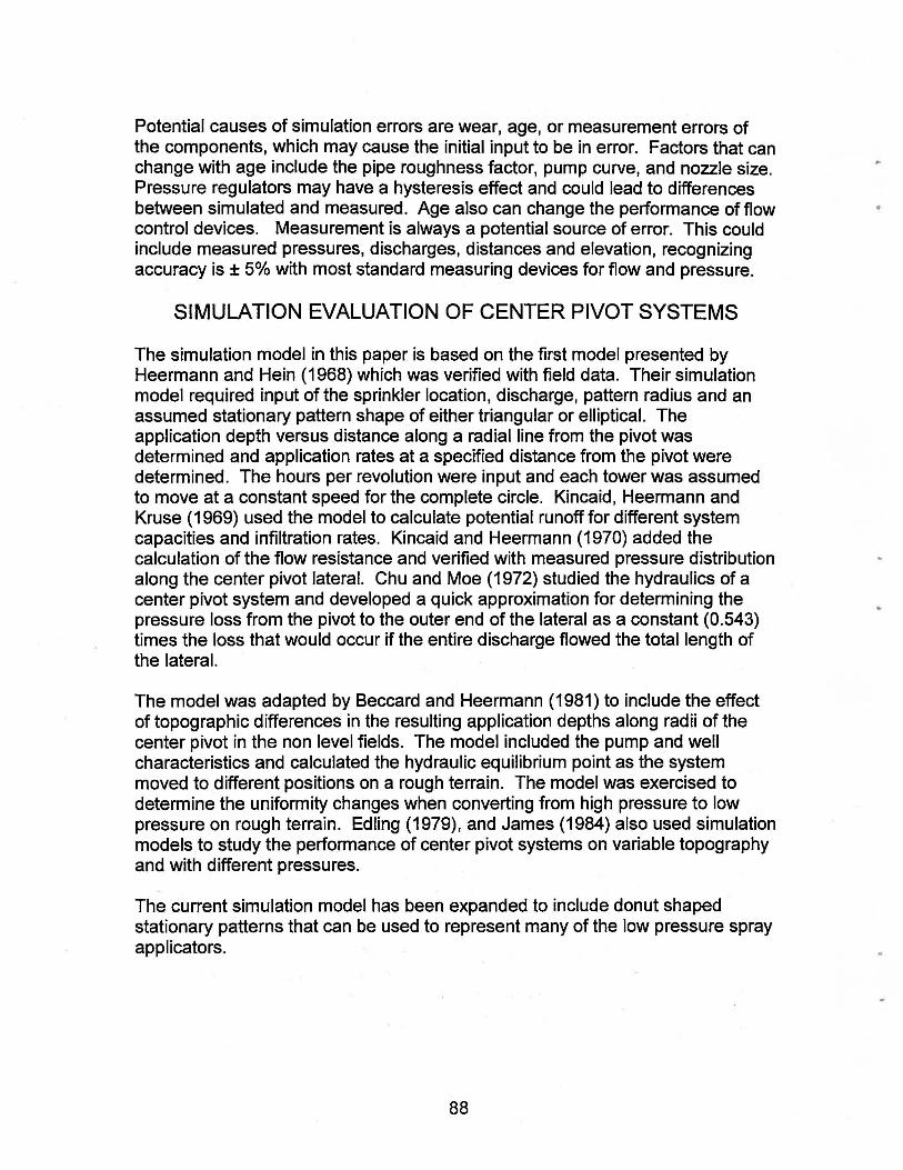
SPRINKLER PATTERN
There are three sprinkler patterns available in the program. They are: triangular, elliptical, and donut. These are associated with the sprinkler model used. In general high pressure single nozzle systems have triangular patterns, dual nozzle systems have elliptical patterns, and low pressure spray systems have a donut pattern. When running the program, specify triangular =1, elliptical = 2, and donut= 3. See Figure 2 .
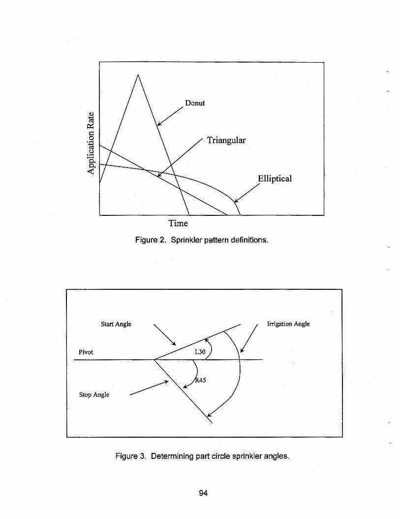
START-STOP ANGLES
The start and stop angles for a part circle sprinkler are defined by imagining standing at the pivot and looking out along the pipe. Check if the sprinkler starts on the right or left. Then using the pipe as the zero reference point, measure the angle back toward the pivot. Use the same technique for the stop angle. All angles are positive and between O and 180 degrees. See Figure 3.
93
o1eUuoneo1IooV /Donut
Time
Figure 2. Sprinkler pattern definitions.
Start Angle
Pivot
Stop Angle
/ Irrigation Angle
Figure 3. Determining part circle sprinkler angles.
94

RUNNING THE SIMULATION
Once the System File is complete, the simulation can be run. A few parameters are entered at runtime.
1. Hours/Rev - The time needed to complete one revolution of the Pivot. This directly determines how much water is applied.
2. Sprinkler Number - The program can simulate the water application from either 1 specific sprinkler, or the overlap of all sprinklers on the system. To simulate one sprinkler, enter the number of the sprinkler. To simulate all sprinklers, enter All.
3. Starting Distance for depth simulation (ft.).
4. Stopping Distance for depth simulation (ft.).
5. Distance Increment - The distance between the simulated catch cans (ft.).
6. The Minimum Depth for Uniformity (in.)
Once these parameters are entered, start the simulation.
RESULTS
As the simulation runs, depths vs distance are plotted on the screen. Once the simulation is completed, the simulated depths and the overall system information are provided. Overall system information includes:
1. The head per .stage of the pump - gpm 2. The pivot pressure - psi 3. The system discharge based on the pump curve - gpm 4. The system discharge based on all the integrated depths - gpm 5. The system discharge based on all depths above the minimum depth -
gpm 6. The effective irrigated area, which is the area receiving water above
the minimum depth - acres 7. The mean depth - in. (of all depths above the minimum) 8. Christiansen's uniformity coefficient (of all depths above the minimum) 9. Mean low quarter uniformity (of all depths above the minimum) 10. Plot of depth vs distance
95

The information that is available for each sprinkler is:
1. The line pressure - psi 2. The nozzle pressure - psi 3. The discharge - gpm 4. The pattern radius - ft
The applicatior-i depths are the final piece of information provided. They are listed by distance.
CATCH CAN DATA
In addition to simulating a Center pivot system and analyzing it's uniformity, Catch Can data can be entered for uniformity analysis, and saved for future comparisons.
DISCUSSION OF EVALUATION PROCEDURES
Evaluations of center pivot simulations were compared against catch can spacing (Heermann and Spofford, 1998). Catch can data had significantly more variation than the simulated values but approximately the same average depths. The sprinklers were spray nozzles with deep grooved pads producing distinct streams and large drop sizes. The catch can test was repeated on the same system by replacing the pads with smooth pads. The catch can CU increased by 10% when changing from the deep grooved pads to the smooth pads. The distinct streams are not measured correctly with small (10-20 cm) catch cans.
The particular objective for evaluating a center pivot system should be considered when selecting the evaluation procedure. If the objective is to consider modifications to improve the uniformity, there is a distinct advantage in using the simulation model procedure. Once the distribution uniformities are calculated with the existing system, it is quite simple to propose changes and simulate the improvements.
Disadv.fil1t迫es of catch cans Wind Night Testing Evaporation Difficulty in catching streams from grooved pads Small pattern radii - large number of cans Extreme care to set cans level and at proper distance Labor intensive
96

c
Advan~ Provides visual real field data of actual conditions Simple to install More readily accepted by user or system owner Does not need a computer
Disadv~ Difficult to obtain pump curves Difficult to obtain elevation data. Requires labor to verify field installation Need drawdown water level Must have understanding of running models May need additional measurements if simulation disagrees with field data Need to know pattern shapes for application devices
Advan~ Less labor intensive to obtain field pressure and discharge data Wind is not a problem Provides a complete hydraulic analysis for comparison with field data Measurement errors of catch cans eliminated Modification or design can easily be evaluated Used to analyze for potential problems Aids in identifying pump problems Allows analysis of changing drawdown Successive runs with water table changes Can be used to recommend design changes Analyze effects of elevation change$ for a particular field Analyze effect of big-gun operation
CONCLUSION
Simulation models can effectively be used in the evaluation ofcenterp.ivot systems. Advantage of a simulation procedure is the speed of evaluation of an existing system and system modifications. The simulation model can also be used to determine the distribution over the entire field as the topography varies and big gun sprinklers are turned on and off. It also can be an effective tool for diagnosing distribution problems of a center pivot system. Procedures need to be developed to effectively use the simulation for detecting and interpreting the cause of differences between the field measured and simulated system pressure and discharge.
REFERENCES
ASAE Standards. 1999. ASAE S346.1 test procedure for determining the uniformity of water distribution of center pivot, corner pivot, and moving lateral irrigation machines equipped with spray or sprinkler nozzles. American Society of Agricultural Engineers.
97

Beccard, R.W. and D.F. Heermann. 1981 . Performance of pumping plant-center pivot sprinkler irrigation systems. ASAE Paper 81-2548, St. Joseph Ml.
Bremond, B. and B. Molle. 1995. Characterization of rainfall under center pivot: influence of measuring procedure. Journal of Irrigation and Drainage Engineering, ASCE, Vol. 121(5):347-353.
Christiansen, J. E. 1942. Irrigation by sprinkling. California Agric. Expt. Station Bull. No.570.
Chu, T.S. and D.L. Moe. 1972. Hydraulics of a center pivot system. Trans. of the ASAE 15(5):894,896.
Duke, H.R., Heermann, D.F., Dawson, L.J. 1992. Appropriate depths of application for scheduling center pivot irrigations. Trans. of ASAE 35(5):1457-1464.
Edling, R.J. 1979. Variation of center pivot operation with field slope. Trans. of ASAE 15(5): 1039-1043.
Hart, W.E., and D.F. Heermann. 1976. Evaluating water distribution of sprinkler irrigation systems. Colorado State University Tech. Bull. 128, June. 42 pp.
Heermann, D. F. and P. R. Hein. 1968. Performance characteristics of the self-propelled center pivot sprinkler irrigation system. Trans. ASAE 11 (1): 11-15.
Heermann, D.F. and T.L. Spofford. 1998. Evaluating center pivot irrigation systems. ASAE Paper 98-2068. St. Joseph, Ml.
James, LG. 1984. Effects of pump selection and terrain of center pivot performance. Trans. of ASAE 27(1):64-68,72.
Kincaid, D.C., D.F. Heermann, and E.G. Kruse. 1969. Application rates and runoff center-pivot sprinkler irrigation. Trans. the ASAE 12(5):790-794,797.
Kincaid, D.C. and D.F. Heermann. 1970. Pressure distribution on a center-pivot sprinkler irrigation system. Trans. of the ASAE 13(5):556-558.
Livingston, P., J.C. Loftis, and H.R. Duke. 1985. A wind tunnel study of sprinkler catchcan performance. Trans. ASAE 28(6):1961-1965.
National Engineering Handbook. 1983. Section 15, Irrigation, Chapter 11, Sprinkle irrigation. United States Department of Agriculture, Soil Conservation Service. (Now Natural Resources Conservation Service).
Warrick, AW. 1983. Interrelationships of irrigation uniformity terms. Journal of lrrig. And Drain. Engr. 109(3):317-332,
98
矗


![Gen-X 10 LE - teamcrc.comGen-X 10 LE. 1 Center Pivot Base Alum Pivot ball 2-56 Button Head Assemble the Molded Center Pivot assembly as shown. Tighten the 2-56 button head screws [4]](https://static.fdocuments.us/doc/165x107/600a6ea296d1e569916acb20/gen-x-10-le-gen-x-10-le-1-center-pivot-base-alum-pivot-ball-2-56-button-head.jpg)