Bulletin Number 89-4

ECONOMIC DEVELOPMENT CENTERS.. .. .daft,

,- --- ^ ' -A

WEALTH, WEATHER RISK ANDTHE COMPOSITION AND PROFITABILITY:

OF AGRICULTURAL INVESTMENTS

Mark R. Rosenzweig

Hans P. Binswanger

ECONOMIC DEVELOPMENT CENTER

Department of Economics, Minneapolis

Department of Agricultural and Applied Economics, St. Paul

UNIVERSITY OF MINNESOTA

June, 1989

Wealth, Weather Risk and the Composition

and Profitability of Agricultural Investments

Mark R.

University

Rosenzweig

of Minnesota

Hans P. Binswanger

The World Bank

June 1989

A major issue in the literature concerned with economic development has

been the relationship between average productivity and the distribution of

wealth, in particular the distribution of land. Attention has primarily

been focused on how features of rural labor markets in low-income settings,

inclusive of market segmentation and nutrition-wage interactions, entail

efficiency gains from an equalizing redistribution of land (e.g., Mazumdar,

1977; Dasgutpa and Ray, 1984). These concerns have in part spawned a large

number of empirical tests of technical scale economies (e.g., Bardhan,

1973), farm household "separability" (Lopez, 1986; Pitt and Rosenzweig,

1986; Benjamin, 1988), and health-wage associations (Behrman and Deolalikar,

1987).

Studies related to the distribution-efficiency issue in the context of

low-income rural areas have tended to ignore risk considerations, although

the advantages of large landowners in obtaining credit has been recognized

(Sen, 1966). Despite the growing evidence that farmers in low-income

environments are characterized by aversion to risk (Moscardi and deJanvry,

1977; Dillon and Scandizzo, 1978; Binswanger, 1980, Antle, 1987), however,

there has been little empirical evidence on the importance of risk in

shaping the actual allocation of production resources among farmers

differentiated by wealth.1 Empirical work on contractual relations in low-

income rural areas has also not been successful in obtaining credible or

consistent empirical relationships between wealth and risk behavior (Bell

and Srinivasan, 1985), in part because of population heterogeneity in risk

attitudes.

While it might be thought that a principle impediment to obtaining

better evidence on risk-related behavior in low-income countries is the

unavailability of data, an advantage almost unique to the study of

agricultural environments is that one of the major sources of risk, weather,

has been recorded for long periods of time in most countries of the world.

Despite this, the literature on agricultural risk has not exploited actual

weather data to measure risk, although rainfall information has been

fruitfully used to study intertemporal consumption behavior (Wolpin, 1982;

Paxson, 1988).

In this paper we utilize unique panel data from rural India on

investments, wealth and rainfall to examine how the composition of

productive and non-productive asset holdings varies across farmers with

different overall levels of total wealth holdings and across farmers facing

different degrees of weather risk. In particular, we propose and implement

a test of the central feature of an investment equilibrium characterized by

risk-averse agents, namely the existence of a positive association between

the average returns to individual production assets and their sensitivity to

weather variability. We also estimate how the influence of weather risk on

asset portfolios and farm profitability varies with measured risk

preferences and with total wealth holdings.

In part one of the paper, we set out a simple framework for exploring

the determination of agricultural investments under risk which explicitly

incorporates the first two moments of the distribution of weather outcomes.

The analysis rests on the estimation of a restricted profit function in

which it is assumed that farmers choose a set of assets differentially

sensitive to weather-variability based on their risk preferences but

allocate resources to maximize profits after the resolution of uncertainty.

Section two contains a description of the data and a discussion of

measurement issues, with particular attention to the measurement of weather.

In section three, the profit function estimates are presented and tests of

scale economies, of the applicability of the two-moment distributional

assumption, and of the risk-aversion investment equilibrium are reported.

In the next section, estimates of the influence of experimentally-

ascertained risk preferences, weather risk and wealth on the riskiness and

profitability of farmers' portfolios of investments are estimated. These

estimates are also used to test for the existence of risk-preference

heterogeneity.

The empirical results reject the hypothesis that the composition of

agricultural investments reflects technical scale economies but support the

hypothesis that asset portfolios are influenced significantly by farmers'

aversion to risk. The results also indicate that the trade-off between

profit variability and average profit returns to wealth is significant and

that the loss in efficiency associated with risk mitigation is considerably

higher among the less wealthy farmers. Average incomes are thus not only

lower but income inequality is exacerbated relative to the distribution of

wealth as a consequence of uninsured weather risk. These results are shown

to be consistent with decreasing relative and absolute risk aversion rather

than solely with wealth-related credit market or other risk diffusion

advantages. However, the results indicate that for farmers in the top

quintile of the wealth distribution, increases in risk do not lead to

reductions in the measured riskiness of investment portfolios and thus to

decreased profits. A wealth-equalizing redistribution of land could thus

increase average profitability, but only if land is acquired from the upper

tail of the wealth distribution, although such a program may be less

efficient than improving access to consumption credit or other means of

insurance.

1. Theoretical Framework

We consider a farmer with total asset holdings W who allocates his n

production assets prior to the realization of a random weather outcome w in

order to maximize his expected utility of consumption. Because we will be

directly estimating the effects on the investment portfolio of measured

characteristics of the distribution of the stochastic variable, it is

particularly convenient to represent the farmer's expected utility rankings

for consumption in terms of his preference ordering over moments of the

consumption distribution. This is so because it is straightforward to map

changes in the moments of the observed stochastic variable (weather) into

changes in these characteristics of the consumption distribution. Moreover,

Meyer (1987) has demonstrated the consistency of the two sets of rankings,

for the first two moments of the distribution of payoffs, when the

stochastic payoff variables differ from each other only by location and

scale parameters. Under this condition, a wide variety of functional forms

for expected utility models are consistent with models incorporating mean-

standard deviation rankings. Since we utilize direct information on the

stochastic variable we will be able to test for this condition.

The farmer maximizes

(1) U - V(c,ac), VP > 0, Va < 0,

where Mc and ac are the mean and standard deviation of consumption. Meyer

has also demonstrated that the quasi-concavity of (1) is sufficient to

guarantee convexity of preferences, so that V V < 0 and V V - V 2'1L ' U aV

0.

The farmer can influence the arguments in (1) by choosing an

appropriate mix of production investments. Normalizing, arbitrarily, by the

4

nth production asset and assuming a profit function linear homogenous (CRS)

in the investment inputs, we can express the relationship between the mean

and standard deviation of farmer profits, yn and an, the productive

investment portfolio vector ai, where the element ai = value share of the

ith investment input in total wealth, and the mean and standard deviation of

the stochastic weather distribution, A and a , respectively, as:

(2) pu = Wf(5i)M , and

(3) a11 - WT(ai)a,, fa' r < 0. 2

Note that in (2) the mean and standard deviation of profits per unit of

wealth are homogenous of degree 0 in total wealth, reflecting the CRS

assumption, but are of degree 1 in the first two moments, respectively, of

the weather distribution. The homogeneity assumption for the weather

variable is similar to most specifications of stochastic output in the

theoretical literature on agricultural risk utilizing the expected utility

framework (see Feder 1977). We have also for simplicity assumed that there

is one source of stochastic variability in profits. It is straightforward

to consider multiple weather shocks, and we test for these below. With one

source of profit variability, F measures the riskiness of the asset stock

composition.

The mean of consumption is given by

(4) u = u"

The mapping of the standard deviation in profits to that of consumption

depends on what is assumed about capital market constraints. If assets

cannot be sold and borrowing is not possible then a c = a11 , while if farmers

are fully insured against income fluctuations, ac - 0. Most likely, the

situation is somewhere in between these extreme cases. Moreover, the

sensitivity of consumption variability to ex post profit variability may

depend on the total level of asset holdings, for which there may be a

limited market and which may serve as collateral for loans. Rosenzweig and

Stark (1989), for example, report that the association between the variances

of intertemporal profits and consumption was significantly lower for Indian

farmers with greater inherited wealth, and Binswanger and Rosenzweig (1986)

report that wealthier Indian farmers were substantially heavier borrowers.

Both of these studies utilized the same survey data to be employed in this

study. Accordingly, we express the relationship between consumption and

profit variability as

(5) acc - (W)j,

with x'(W) < 0.

The set of first order conditions are given by

(6) V f - -Va a, i-,...,n-i i

where fa fi - fn and F,- Fi - Fn, with fj and rj the marginali i J J

contributions of the jth production capital to the mean and standard

deviation, respectively, of profits. Expression (6) indicates that if

farmers are risk-averse and capital assets differ in their contributions to

profit variability (ra / 0), then as long as farmers' incomes are noti

perfectly insured, (0 < K < 1) (mean) profits will be lower than mean profits

would be if farmers maximized (expected) profits, since the profit

maximization condition is f, = 0.i

A readily testable implication of an investment equilibrium

characterized by risk-aversion, embodied in (6), is the existence of a

positive association across all production assets between marginal

contributions to the mean and to the variability of profits, as for any two

assets i and k,

(7) fa /fa - /i k i k

A second implication of imperfectly insured consumption combined with

risk-averse investment behavior that follows from the positive relationship

between r. and f is that a shift to assets that in equilibrium makei i

higher-than-average contributions to profit variability ("risky" assets)

induces a rise in mean profits, since risky assets must have higher average

returns. Farmers more willing or more able to bear risk thus should not

only hold high-r investment portfolios but should exhibit higher average

profits per unit of wealth.

To establish the conditions under which the efficiency and portfolio

riskiness of farmers changes with total wealth holdings and to assess how

the sensitivity of profits to changes in weather risk is altered as wealth

levels increase, we first note, from Meyer (1987):

1. Farmers exhibit decreasing, constant, or increasing relative risk

aversion as R - (Va + Vaaac)V- 1 -(V c + Vac)Va/V2 aVl + bV V-2

- 0.

2. Farmers exhibit decreasing, constant, or increasing absolute risk

-- 2

aversion as A = VV -l V VV/V 2 0.

For simplicity, assume that there are only two types of capital i and j

and that in equilibrium f, and Fa > 0, i.e. investment good i is the riskyi i

asset, and thus high-a i portfolios are both riskier and more profitable. The

effect of a mean-preserving change in the standard deviation of the weather

distribution on the choice of the risky asset is given by:

(8) - - [(Vaif. + Voaa ao)Wr + ara ] 1-da i i i

- -K[SWT + Vr ]l-1

i

where, suppressing subscripts, - Vf +e + Vf2W + Var aa + Vaa ra W

+ 2Va faWaW < 0 by second order conditions.

The first term in brackets in (8), SWT, is the effect on the riskiness

of investment due to a a wealth-independent increase in the variability of

consumption, and is negative; the second bracketed term is negative as long

as ai is the risky asset. Thus, ceteris paribus, when farmers are not fully

insured (xc 4 0) an increase in weather risk reduces the riskiness of their

portfolios of production capital and mean profitability.

The effect of a change in the level of wealth on ai is:

dai daii. i 1

(9) -- -[R + -- a, ']-dW dao

Because of the homogeneity assumptions embodied in (2) and (3), an increase

in wealth increases by the same proportion both the mean and standard

deviation of profits and consumption. It is thus relative risk aversion (R)

that matters in determining the relationship between the profitability or

riskiness of the capital portfolio and total wealth, as shown in (9). The

second term in brackets reflects the extent to which wealth directly reduces

the variability in consumption for given variability in farm profits via the

asset or credit market. Thus, if c' - 0, farmers cannot save or barter,

decreasing relative aversion is necessary and sufficient for wealthier

farmers to be holding more risky portfolios of production capital and to be

more efficient. However, with wealth accumulation being advantageous in the

credit market and/or with asset resale possibilities, so that A' < 0,

decreasing relative risk aversion is not a necessary condition for

consumption riskiness and profitability per unit of wealth to rise with

total wealth.

The relationship between total wealth and the impact of weather

riskiness on the riskiness (and profitability) of the stock of capital

inputs, assuming third derivatives of (1) are small, is given by

(10) d(dai/da~)/dW- -[r,[ a + rS]- 1

i

da.di I1- [-fa A + F wS + araan + bfaa]da i i

K' dai+- [ -- ac'Vara a

/c daw i

In expression (10), both absolute (A) and relative risk aversion

matter. The first bracketed term is positive if a is non-negative, which is

true when farmers are characterized by non-increasing constant relative risk

aversion; similarly, the second bracketed term must be positive if farmers

are characterized by non-increasing absolute and relative risk aversion

(A,a,b > 0) and f and P are concave. The last bracketed term in (10) arises

from the potential effect of wealth in facilitating consumption smoothing ex

post ((' < 0) and contributes unambiguously to wealth diminishing the effect

of weather variability on portfolio riskiness and profitability. Thus, non-

increasing absolute and relative risk aversion are sufficient, but not

necessary, for the investments of wealthier farmers to be less influenced by

weather risk.

2. The Data

The preceding framework indicates that to test for the existence of an

investment equilibrium conditioned by risk and to assess the interactions

between total wealth holdings, agricultural risk and the composition of

investment holdings requires time-series data on investments, wealth and

weather. The ICRISAT Indian village surveys (Singh et al., 1985) provide

detailed time-series information on agricultural production and investments

for farm households over a period of up to ten years. Begun in the crop

year 1975-76 in six villages in three agroclimatic regions of the Indian

semi-arid tropics, the survey collected longitudinal information

approximately every three weeks on all transactions (purchases, sales,

production, investment) for 40 households in each village, 30 of which were

cultivating households. At the conclusion of the survey, there were ten

years of information collected for three of the villages, seven years for

one, and nine years of information for two of the original six villages. In

1980-81, two other villages (each with 40 households) were added to the

survey and were surveyed for four years; another two villages (80

households) were added in 1981-82 and were surveyed for three years.

In addition to the transaction information, in each year on

approximately July 1 a complete inventory of the households' asset holdings

was taken. All of the information was obtained by resident village

investigators. The ICRISAT wealth and investment portfolio data are thus

likely to be substantially more accurate than i:. most surveys, particularly

those occurring at one point in time. As part of the survey, daily rainfall

information was also obtained. It is thus possible to construct a number of

alternative measures of rainfall incidence and variability.

Two other features of the ICRISAT village survey make it particularly

well-suited for studying the consequences of agricultural risk for

investment. First, the separation theorem (Tobin (1958)) does not appear to

10

be applicable to the villages. That is, farmers are not generally able to

invest in a riskless asset. In principle, farmers could alter the riskiness

of their investment portfolios by merely changing the proportion of their

holdings that they lease out at a fixed rental rate, while arranging

productive assets on the self-cultivation portion of their portfolios so as

to maximize profits. In that case, the composition of production portfolios

(but not leasing behavior) would be invariant to risk. While the ICRISAT

data do not provide information on the contractual terms for leased-out

land, in less than seven percent of the observations (household-years) are

farmers renting in any land at fixed rental rates. 3 Very few farmers are

thus able or willing to absorb the risk entailed by taking on a fixed-rent

contract, leaving almost all farmers fully exposed to weather risk. In

approximately 21 percent of the observations, farmers are share renting

land; this contractual form, of course, mitigates but does not eliminate

risk.

A second advantage of the ICRISAT survey is that the farmers in six of

the villages were subject to an experiment designed to directly elicit their

aversion to risk (Binswanger, 1980). It is thus possible to test whether

our non-experimentally obtained measures of portfolio riskiness are related

to these independently-ascertained measures of subjective risk-aversion.

The semi-arid tropics in which the ICRISAT study villages reside are

characterized by very low levels of erratically-distributed rainfall. As a

consequence, agricultural incomes are low and quite variable--in the six

original villages for which there is from seven to ten years of information,

the average coefficient of variation in total farm profits (net of the value

of family labor) was 127. In contrast, our analysis of the earnings of U.S.

white males aged 25-29 in 1971, surveyed in seven rounds of the National

11

Longitudinal Survey of Youth, indicated that the average coefficient of

variation in earnings was only 39. The variability in agricultural income

is not due to technical change; the crops grown in the survey areas -

millet, pigeon-pea, cotton--were not affected by the Indian Green

Revolution. Agricultural risk is thus predominantly weather-based in this

environment, and it is possible to utilize all sample years to estimate the

technology of production.

Finally, total wealth holdings in the six villages are very unequally

distributed. Based on sample-period averages of real wealth for each farm

household, the top 20 percent of farmers own over 54 percent of all wealth.

Mean total wealth holdings (in 1983 rupees) was 54,158 rupees, with a median

of 33,265 rupees. The minimum average value of wealth holdings was 4,154;

the highest was 453,581 rupees. Mean farm profits, also in 1983 rupees, was

5,825.

3. Specification of the Technology and the Measurement of Weather

To estimate the profitability and riskiness of asset portfolios, we

aggregated the detailed information on (annual) asset holdings into nine

categories, by value, using 1983 prices: unirrigated landholdings; irrigated

landholdings, inclusive of the value of irrigation equipment; draft animals,

including bullocks and water buffalo; milk animals; other animals, including

chickens and goats; traditional farm implements, including manual plows,

carts, blades, hoes; modern machinery, including tractors; liquid capital,

including financial assets and food stocks, and consumption assets,

including consumer durables and housing.

To estimate the relationship between the two moments of the weather

distribution and profits, we assume that the profit function is a normalized

quadratic, where we normalize by total wealth holdings. Thus profits for

12

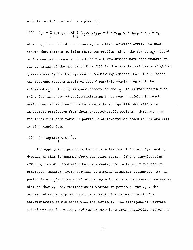
each farmer k in period t are given by

(11) Ukt = 1 iaikt + I 2 Sijaiktojkt + 7iaiktt + Twt + Ekt + Vki i j

where ekt is an i.i.d. error and vk is a time-invariant error. We thus

assume that farmers maximize short-run profits, given the set of ais, based

on the weather outcome realized after all investments have been undertaken.

The advantage of the quadratic form (11) is that statistical tests of global

quasi-concavity (in the ai) can be readily implemented (Lau, 1976), since

the relevant Hessian matrix of second partials consists only of the

estimated 6is. If (11) is quasi-concave in the ai, it is then possible to

solve for the expected profit-maximizing investment portfolio for each

weather environment and thus to measure farmer-specific deviations in

investment portfolios from their expected-profit optimum. Moreover, the

riskiness 1 of each farmer's portfolio of investments based on (3) and (11)

is of a simple form:

(12) F - sqrt((Z 7i i)2)i

The appropriate procedure to obtain estimates of the Pi, 6i, and 7i

depends on what is assumed about the error terms. If the time-invariant

error vk is correlated with the investments, then a farmer fixed effects

estimator (Mundlak, 1978) provides consistent parameter estimates. As the

portfolio of ai's is measured at the beginning of the crop season, we assume

that neither wt, the realization of weather in period t, nor ekt, the

unobserved shock to production, is known to the farmer prior to the

implementation of his asset plan for period t. The orthogonality between

actual weather in period t and the ex ante investment portfolio, net of the

13

permanent distributional characteristics of weather, is testable and we test

it below.

The remaining issue in obtaining estimates of the technology parameters

is the characterization of weather. We take an empirical approach. We used

the daily rainfall information to construct six measures of rainfall: the

beginning and end dates of the rainy season (monsoon), where the monsoon

onset is determined as the date after which there has been at least 20 mm of

rain within several consecutive days after June 1; the fraction of days

within the season with rain; the average rain per day during the season, and

the length of up to two intraseasonal drought periods. Village "folklore"

suggests that the timing of the monsoon is the most important aspect of

weather (and uncertainty). We therefore first regressed total (real)

profits from crop production and total farm profits (crop profits plus

profits from animal by-products) on the monsoon onset date and then on all

six weather variables, using all farm households in the ten ICRISAT

villages.

Random effects estimates of the influence of the rainfall variables on

profits are presented in Table 1. The initiation date of the monsoon does

significantly affect both crop and total profits--a one standard deviation

delay (16 days) in the start of the monsoon reduces crop (total) profits by

222 (150) rupees, or by approximately 6 (3) percent. We could not reject

the hypothesis that the five other measures of rainfall, included in the

specification reported in the second column for each profit variable, do not

add to the explanatory power of the profit regressions. Moreover, inclusion

of the other rainfall variables does not appreciably alter the effect of the

onset variable. Of the other rainfall measures, the only potentially

important candidate is the fraction of days with rain. Accordingly, we use

14

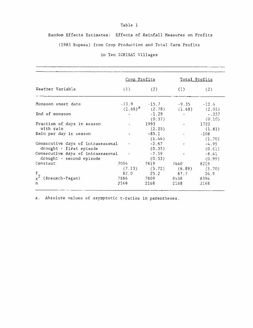
Table 1

Random Effects Estimates: Effects of Rainfall Measures on Profits

(1983 Rupees) from Crop Production and Total Farm Profits

in Ten ICRISAT Villages

Crop Profits Total Profits

Weather Variable (1) (2) (1) (2)

Monsoon onset date -13.9 -15.7 -9.35 -12.4(2 .6 8)

a (2.78) (1.68) (2.05)End of monsoon - -1.29 - -.357

(0.37) (0.10)Fraction of days in season - 1993 - 1722with rain (2.25) (1.81)

Rain per day in season - -85.1 - -108(1.44) (1.70)

Consecutive days of intraseasonal - -2.67 - -4.95drought - first episode (0.35) (0.61)

Consecutive days of intraseasonal - -2.59 - -8.41drought - second episode (0.33) (0.99)

Constant 7054 7619 7440 8219(7.13) (5.72) (6.89) (5.70)

F 82.0 25.2 87.7 26.92 (Breusch-Pagan) 7886 7809 8438 8394

n 2168 2168 2168 2168

a. Absolute values of asymptotic t-ratios in parentheses.

both this measure of rainfall and the onset date as weather variables in our

estimation of (11), and undertake additional tests of their importance.

That the quantity of rainfall is far less important than its timing is

consistent with the well-known difficulties experienced by researchers using

rainfall quantities to explain yield (Herdt, 1972) or the allocative

behavior of farmers (McGuirk and Boissert, 1988) based on aggregate Indian

data.4

The village-level rainfall variables explain a small proportion of the

variability in individual profits. This might suggest that an investigation

of the influence of the riskiness of these variables on farmer behavior

would not yield significant results--unmeasured variability in profits, due

to sources orthogonal to rainfall, might be a far more important source of

risk. However, even if all of the residual variability in profits were not

merely measurement error, it is not necessarily true that such variability

significantly alters behavior. To the extent that non-weather-induced

income variability is not covariant across farmers within the village, such

risk might be considerably mitigated ex post by utilizing locally-supplied

credit or via other village-based risk-sharing arrangements. Binswanger and

Rosenzweig (1987) have shown that most loans in the ICRISAT villages are

acquired from local informal sources without access to external funds.

Moreover, loans appear to be less available when the local economy is

subject to a common shock, such as a late monsoon (Rosenzweig, 1988). Thus

weather-induced profit variability may be far less insurable than

idiosyncratic or household-specific profit variability, necessitating ex

ante risk reduction through altering the portfolio of investments

differentially sensitive to weather outcomes. Investments would then be

predominantly responsive to weather risk.

15

To assess the relative importance of weather-induced and other sources

of income variability on consumption, we utilized the information on

household food consumption (85 percent of total consumption) that is

available for nine years in three of the ICRISAT villages. In column (1) of

Table 2 we report a fixed effects regression of food consumption on total

farm profits and the age of the household head. The results indicate that

household (food) consumption is not wholly independent of current farm

profits--a 100 rupee decrease in profits reduces food consumption by seven

rupees. In the second column of Table 2 we regress, again using fixed

effects, food consumption on farm profits measured net of the effects of the

weather variables. This profit measure is the residual obtained from the

regression of farm profits on the weather variables. These profit-weather

regressions were run separately for each household, since the risk framework

suggests that weather should differentially affect profits according to the

individual farmer's composition of assets ai. This residual measure of

household-specific income, orthogonal to income determined by the weather,

has an effect on food consumption that is only .6 of a percent that of

actual profits. Common weather shocks to income appear to have

substantially greater consequences for consumption than does idiosyncratic

risk. 5

4. Estimates of the Technology and Tests of the Risk-Aversion Investment

Equilibrium

Table 3 reports some test statistics based on our estimates of the

normalized restricted profit function (11). We included in the

specification, in addition to the eight investment types (excluding consumer

durables as part of the normalization) and the two weather measures, total

wealth and its square, to test for scale effects, the number of adult male

16

Table 2

Fixed Effects Estimates: Effects of Total Farm Profits, Inclusive and

Exclusive of the Effects of Weather, on Food Consumption

in Three ICRISAT Villages, 1975-1984

Variable (1) (2)

Age of household head -85.5 -71.9( 1 . 5 3 )a (1.35)

Age squared .438 .373(0.78) (0.70)

Farm profits .0694(5.76)

Farm profits net of effects of .00047weatherb (0.02)

F 13.6 2.86n 720 720

a.

b.

Absolute values of asymptotic t-ratios in parentheses.

Residual from household-specific fixed-effects regression of total farmprofits on onset of monsoon in the village.

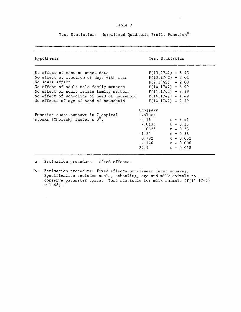
Table 3

Test Statistics: Normalized Quadratic Profit Function a

Hypothesis

NoNoNoNoNoNoNo

Test Statistics

effect of monsoon onset dateeffect of fraction of days with rainscale effecteffect of adult male family memberseffect of adult female family memberseffect of schooling of head of householdeffects of age of head of household

Function quasi-concave in 7 capitalstocks (Cholesky factor < 0b)

F(13,1742)F(13,1742)F(2,1742)F(14,1742)F(14,1742)F(14,1742)F(14,1742)

CholeskyValues-2.16-.0133-.0623

-1.240.792-.146

27.9

ttttttt

a. Estimation procedure: fixed effects.

b. Estimation procedure: fixed effects non-linear least squares.Specification excludes scale, schooling, age and milk animals toconserve parameter space. Test statistic for milk animals (F(14,1742)= 1.68).

6.732.012.096.993.39

1.492.79

3.410.330.330.360.0320.0060.018

and female family members, and the schooling and age of the household head.

The test statistics indicate the timing of the monsoon has a statistically

significant effect on total farm profitability, while the set of 13

coefficients associated with the proportion of days with rain is not

statistically significant at even the ten percent level. In subsequent

tests, therefore, we only consider the influence of the monsoon onset

variable.

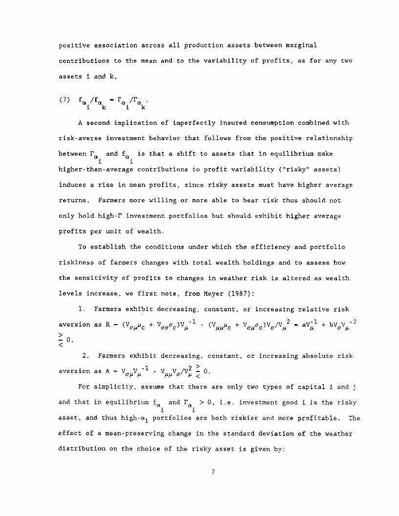
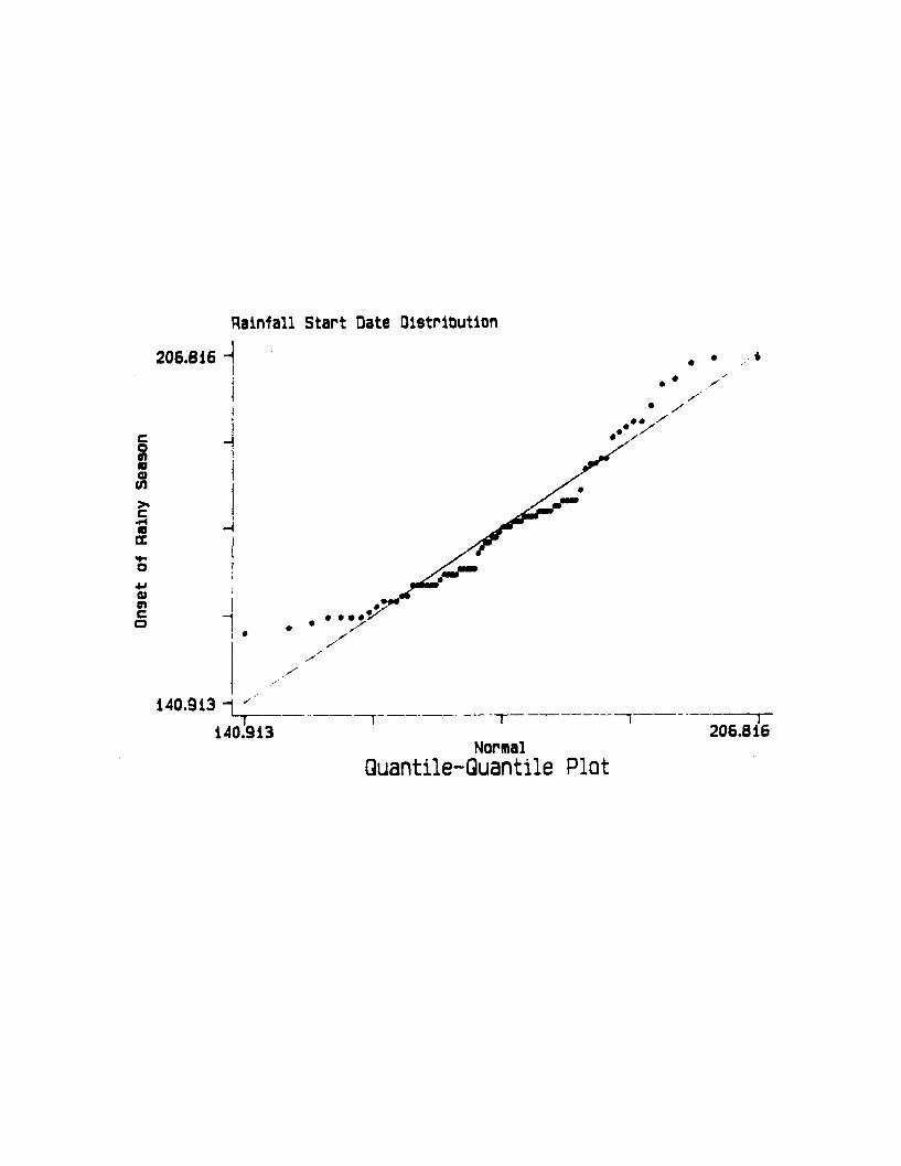
Does the principle measured risk variable, the monsoon onset date,

conform to the location and scale transform assumption of the mean-standard

deviation analysis of risk? As noted, if the onset date is normally

distributed, this property holds. Figure 1 presents a normal quantile plot

of this rainfall measure, based on 75 observations. The plot suggests some

conformity to the normal, with perhaps fatter tails. The Kolmogorov-Smirnov

test statistic is .119, which is only statistically significant at the 20

percent level of significance. We thus cannot reject the assumption that

the monsoon onset date has a normal distribution.

Of the other test statistics, the results indicate the absence of

technological scale effects on profits. Differences in investment

portfolios across wealth classes evidently do not arise from technical scale

economies. The results also indicate that schooling has no effects on

profits, but reject the hypothesis that the age of the farmer does not

affect profits (the marginal return is positive at sample mean values).

These latter results are consistent with the hypothesis that in environments

subject to risk but characterized by stationarity, experience, but not

formal schooling, has real payoffs, as found in Rosenzweig and Wolpin

(1985). The tests also reject the hypothesis that the size of the family

labor force does not influence profits. This result appears to contradict

17

Rainfall Start Date DistributionOr aic j

C

0c

0

4JGJ

A A% APJ ~A

0

* /

S*

7

14U.t1-1 -IT- -- _ --_ _ _- T I . __----- ]V

140.913 206.816Normal

Quantile-Quantile Plot

li

the findings by Pitt and Rosenzweig (1986) and by Benjamin (1988), based on

Indonesian data, indicating the perfect substitutability of hired and family

labor.6

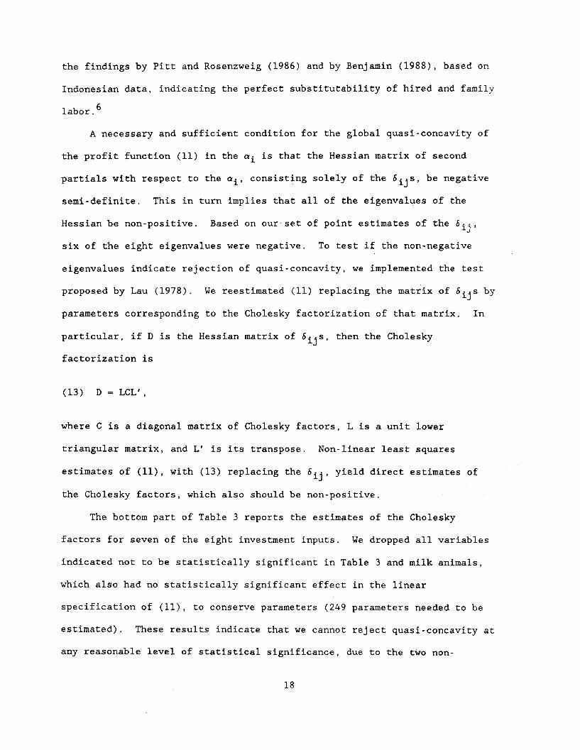
A necessary and sufficient condition for the global quasi-concavity of

the profit function (11) in the ai is that the Hessian matrix of second

partials with respect to the ai, consisting solely of the 6 ijs, be negative

semi-definite. This in turn implies that all of the eigenvalues of the

Hessian be non-positive. Based on our set of point estimates of the 6ij,

six of the eight eigenvalues were negative. To test if the non-negative

eigenvalues indicate rejection of quasi-concavity, we implemented the test

proposed by Lau (1978). We reestimated (11) replacing the matrix of Sijs by

parameters corresponding to the Cholesky factorization of that matrix. In

particular, if D is the Hessian matrix of 6ijs, then the Cholesky

factorization is

(13) D - LCL',

where C is a diagonal matrix of Cholesky factors, L is a unit lower

triangular matrix, and L' is its transpose. Non-linear least squares

estimates of (11), with (13) replacing the 6ij, yield direct estimates of

the Cholesky factors, which also should be non-positive.

The bottom part of Table 3 reports the estimates of the Cholesky

factors for seven of the eight investment inputs. We dropped all variables

indicated not to be statistically significant in Table 3 and milk animals,

which also had no statistically significant effect in the linear

specification of (11), to conserve parameters (249 parameters needed to be

estimated). These results indicate that we cannot reject quasi-concavity at

any reasonable level of statistical significance, due to the two non-

18

negative Cholesky factors being measured with very little precision.

However, our point estimates of the 6ij make it impossible to find a set of

ai that maximize expected profits.

In Table 4 we present the computed marginal profit level effects,

evaluated at the sample means, and the marginal profit variance effects,

with their associated asymptotic t-ratios, for all eight investment inputs

based on the normalized profit function parameter estimates. Sample mean

investment shares are reported in the leftmost column, with their standard

deviations. All estimated effects, reported in columns two and three, are

relative to the effects of consumer durables and housing. The results

reject the hypothesis that the investment inputs have identical profit

variance or profit level effects. The Spearman rank correlation across the

eight types of capital stocks between level and variance effects is

positive, in conformity to expression (6), but not statistically significant

at the 15 percent level. The principle deviants from the risk-aversion

investment equilibrium condition are the liquid assets and draft animal

categories--there appears to be severe underinvestment in both assets

despite their not contributing, on the margin, to increasing profit

variability. Exclusion of draft animals leads to a rank correlation between

level and variability effects of .68, which is statistically significant at

the .01 level. Exclusion of both draft animals and liquid assets yields a

rank correlation of .83, which is also statistically significant at the .01

level.

What may account for the underinvestment in both liquid assets and

draft animals? The framework set out in section 1 does not accommodate the

possibility that specific capital items may be more or less useful in

smoothing consumption ex post. With the x-function having as arguments not

19

Table 4

Estimated Normalized Profit Level and Profit Variance Effects of

Changes in the Shares of Productive Capital Items

Relative to Consumer Durable and Housing Wealtha

Share of Total Marginal Profit Level Marginal Profit Var-Capital Item Wealth (ai) Effect (8a/8a i) iance Effect (Par /ai)

Irrigated land 0.132 0.0656 0.0645(0.226)b (2 .4 5)c (0.80)c

Dry land 0.591 0.0289 -.0496

(0.317) (1.62) (0.78)Traditional imple- 0.0073 1.285 1.184ments (0.013) (3.87) (1.20)

Modern implements 0.00376 0.127 3.891(0.0403) (0.63) (8.86)

Draft animals 0.0223 1.167 -0.644(0.0312) (10.6) (1.34)

Milk animals 0.0249 0.00234 -0.152(0.0433) (0.02) (0.47)

Other livestock 0.0174 0.156 0.568(0.0381) (1.35) (2.39)

Liquid assets 0.0806 0.0928 -2.45(0.0826) (2.22) (1.40)

Consumer durables 0.121and housing

Spearman rank correlation, .262level and variance effects

Spearman rank correlation, .679excluding draft animals

Spearman rank correlation, .829excluding draft animals and liquid assets

a. Computed from normalized restricted profit function estimates at samplemeans of ai .

b. Standard deviation in parentheses in column.

c. Absolute values of asymptotic t-ratios in parentheses in column.

only total wealth but ai as well, the equilibrium condition (6) becomes

(6') V f -= VOa[a + ar].i i i

If (6') is the correct characterization of the equilibrium, then without

prior knowledge of the association between the profit variability and ex

post consumption smoothing effects K for each ai, it is no longer possiblei

to know how profit level and profit variability effects will be correlated.

It is not surprising that liquid assets (financial assets and food

stocks) play a role in smoothing consumption as well as provide a source of

funds for purchasing variable inputs. However, our analysis of the

transaction records from the original six villages covering the entire

survey period also indicates that the purchase and sale of draft animals

accounted for 72.9 percent of all market transactions involving investment

durables. The high turnover rate for draft animals suggests that this

capital item may also be playing a role in consumption smoothing predominant

among the other durable agricultural stocks. If so, then in periods in

which weather has been particularly poor, both the level of liquid assets

and stocks of draft animals may be depleted and thus exhibit high marginal

profit level returns. For given profit variability effects, however,

overinvestment in conventionally-characterized liquid assets and in draft

animals in normal periods may be observed, given their consumption smoothing

role. An investigation of optimal stock behavior is beyond the scope of

this paper, but is considered in Rosenzweig and Wolpin (1989) in the context

of a dynamic stochastic model.

5. Weather Risk, Wealth and the Riskiness and Profitability of Farm

Investment Portfolios

20

Based on the estimates of the profit function and the actual asset

portfolios ai of the household we can construct individual measures of

portfolio riskiness r, from (13), for each farm household. There is

considerable inter-household variability in F--based on survey-period

averages for each household, the sample mean of F is .000632 and the

standard deviation is .000539. At the sample mean of wealth, the mean

estimate of r implies an average standard deviation in total profits of 544

rupees at the mean standard deviation of the monsoon onset; the average

coefficient of variation in profits associated with the average F measure of

portfolio weather sensitivity is thus 9.3. At the same (mean) wealth level,

a one standard deviation increase in r raises the coefficient of variation

of profits to 17.3.

To directly assess whether portfolio riskiness and profitability per

unit of wealth are positively associated in the sample, as should be true in

the risk-averse investment equilibrium, we regressed, using fixed effects,

farm profits divided by total wealth (H/W) on the r measure of riskiness and

the farmer's age and age squared. The results were:

(14) II/W - 5.54 r + .00593-age - .000056-age squared(4.31) (2.36) (2.24) n - 2130 F(3,1825) - 8.54

where t-ratios are in parentheses. Farm households with production asset

portfolios less sensitive to weather variability sacrifice profitability, in

conformity to the investment risk framework--a one standard deviation

decrease in portfolio riskiness lowers average profits by 162 rupees at the

mean level of wealth.

The risk framework suggests that the variation in portfolio riskiness

across farm households and over time should be related to the first two

moments of the weather distribution and to total wealth. Moreover, the

21

Determinants of Gamma

Table 5

5(xlO ): Six ICRISAT Villages

Variable/ Random Random Fixed Random RandomEstimation Procedure Effects Effects Effects Effects Effects

Coefficient of varia-tion in onset (CV)

CV-total wealth (x10l4 )

CV. inherited wealth(x10 4 )

Total wealth (x10l4 )

Inherited wealth (x10l4 )

Mean onset date

Risk aversion parameter

CV.risk aversionparameter

Age

Constant

F2 (Breusch-Pagan)2 (Hausman)

-. 884(4. 1 4 )a

.133(7.68)

-7.10(5.72)

.471(0.26)

.590(1.72)76.3(2.13)42.9

328.8103.0

-.267

(0.76).138

(7.75)

-7.07(5.63)

.368(0.20)7.50

(1.27)-.138

(1.89).432

(1.26)33.0(0.72)16.8

287.899.9

.0693(6.30)

-4.13(4.93)

.351(1.64)

8.80

-.551

(2.85)

.0731(5.32)

-5.13(4.78)

.132(0.08)

.490(1.57)69.1(2.13)43.8

176.50.74

-. 0783(0.27)

.0834(6.07)

-5.69(5.32)

.130(0.08)6.33

(1.25)-.102

(1.66).299

(0.99)36.9(0.95)20.3

117.44.51

a. Absolute values of asymptotic t-ratios in parentheses.

effect of a mean-preserving shift in the standard deviation of weather on

portfolio riskiness and profitability may depend on the total level of

wealth holdings. A problem with testing for wealth effects is that at any

given point in time both accumulated wealth as well as the investment

portfolio will reflect the farm household's subjective risk preferences,

which, as shown in Binswanger (1980), vary across the farmers in our sample.

The observed cross-household association between wealth and the risk

characteristics of the asset portfolio, given heterogeneity in risk

preferences, does not conform to the result that would be obtained by

randomly assigning wealth levels across farmers. To the extent that

preferences for risk are time-invariant, a fixed effects procedure will

provide consistent estimates of wealth effects on portfolio allocations.

However, because the moments of the weather distribution are also time-

invariant (under stationarity), use of the fixed effects procedure does not

allow the identification of the direct effects of the characteristics of the

weather distribution on portfolio choice.

The ICRISAT data allow two alternative procedures that may circumvent

the bias due to risk-preference heterogeneity. First, we can exploit the

farmer-specific measures of (partial) risk aversion revealed in the

experimental lottery games reported in Binswanger (1980); that is, we can

treat risk preferences as observables and "control" for them. An

alternative procedure is to use inherited wealth, also available in the

data, instead of current wealth. To the extent that the wealth inherited by

a farmer is orthogonal to his preferences for risk, use of inherited rather

than current wealth reduces biases associated with heterogeneity.

In Table 5 we report reduced-form estimates of the effects on portfolio

riskiness r of changes in the village-specific mean and coefficient of

22

variation (CV) of the monsoon onset date, household total wealth and the

onset CV interacted with wealth, based on the data from the six original

villages where the longer time-series of weather are available. In the

first column, the coefficients obtained using the random effects estimation

procedure are reported. The results conform to the risk-aversion model in

which farmers are characterized by decreasing relative risk aversion and/or

in which wealth contributes to ex post consumption smoothing. At the sample

median of wealth, an increase in the onset CV significantly decreases

portfolio riskiness--a one standard deviation increase in the CV (29.5)

lowers r by 20 percent. The set of coefficients also indicate that the

effect of the weather CV on portfolio riskiness declines sharply with

wealth--at the mean wealth level, F is lowered by only 7.6 percent when the

CV is higher by one standard deviation. Indeed, above wealth levels

corresponding to the top quintile of the wealth distribution (75,376

rupees), there is no negative effect of weather variability on portfolio

riskiness. The top 20 percent of farm households are evidently able or

willing to completely absorb profit risk.

The Hausman test indicates rejection of the hypothesis that the right-

hand-side variables in the specification reported in the first column of

Table 5 are uncorrelated with the residual. In the second column we report

estimates that attempt to correct for preference heterogeneity by including

the measure of each farmer's partial risk aversion parameter, from the five

rupees level in game nine reported in Binswanger (1980). These estimates

are similar to those obtained without the risk preference measures. They

also provide support for the hypothesis that the investment portfolio is

related to preferences for risk. At the sample mean of the onset CV,

farmers with greater aversion to risk according to the experimental games do

23

have lower-P investment portfolios, and increases in the variability in the

start of the monsoon induces more risk-averse farmers to lower the riskiness

of their portfolios more strongly than less risk-averse farmers. However,

the Hausman test statistic still indicates the existence of heterogeneity

bias.

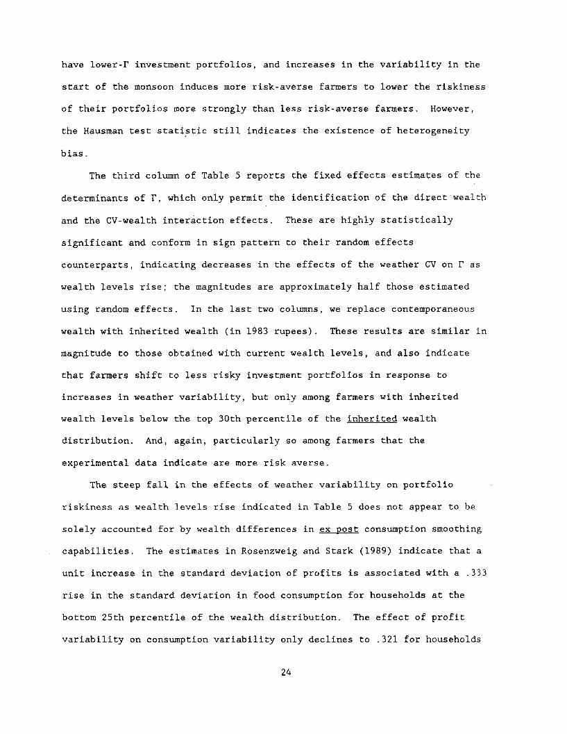
The third column of Table 5 reports the fixed effects estimates of the

determinants of F, which only permit the identification of the direct wealth

and the CV-wealth interaction effects. These are highly statistically

significant and conform in sign pattern to their random effects

counterparts, indicating decreases in the effects of the weather CV on F as

wealth levels rise; the magnitudes are approximately half those estimated

using random effects. In the last two columns, we replace contemporaneous

wealth with inherited wealth (in 1983 rupees). These results are similar in

magnitude to those obtained with current wealth levels, and also indicate

that farmers shift to less risky investment portfolios in response to

increases in weather variability, but only among farmers with inherited

wealth levels below the top 30th percentile of the inherited wealth

distribution. And, again, particularly so among farmers that the

experimental data indicate are more risk averse.

The steep fall in the effects of weather variability on portfolio

riskiness as wealth levels rise indicated in Table 5 does not appear to be

solely accounted for by wealth differences in ex post consumption smoothing

capabilities. The estimates in Rosenzweig and Stark (1989) indicate that a

unit increase in the standard deviation of profits is associated with a .333

rise in the standard deviation in food consumption for households at the

bottom 25th percentile of the wealth distribution. The effect of profit

variability on consumption variability only declines to .321 for households

24

at the top 80th percentile. While this fall in the sensitivity of

consumption to profit volatility by wealth level is statistically

significant, it cannot account for our findings of a steep decline in the

response of the weather sensitivity of investment portfolios to weather

variability as wealth levels increase. The estimates of Table 5 thus

suggest that farmers are characterized by decreasing relative risk aversion.

Although we cannot compute the profit-maximizing portfolio based on the

profit-function parameter estimates, as discussed, we can estimate the

reduced-form relationships between farm profits, weather variability, and

wealth using the same procedures as employed in obtaining estimates of the

determinants of portfolio riskiness. And the equilibrium condition (6)

implies that the coefficient sign patterns for profits should be the same as

those for r. Table 6 reports the estimates of the reduced-form determinants

of profits. The specifications employed in obtaining the profit estimates

are identical to those in Table 5 except that the current-year onset date is

also included, since the current weather state affects profits (but not the

pre-season composition of assets). 8

In the specifications employing contemporaneous wealth levels, the

coefficient estimates are similar in sign patterns to those of Table 5. The

estimates appear to be robust to estimation procedure, however. In

particular, the CV-wealth interaction and onset date coefficients are almost

identical when estimated using random or fixed effects, and the Hausman test

indicates only marginal rejection (.06 level) of the hypothesis that

heterogeneity may be biasing the set of profit-level coefficients, in

contrast to the strong rejection for the r estimates. The experimentally-

obtained risk aversion variables also do not appear to be related to

profits.

25

Table 6

Determinants of Profit Levels: Six ICRISAT Villages

Variable/ Random Random Fixed Random RandomEstimation Procedure Effects Effects Effects Effects Effects

Coefficient of varia- -24.7tion in onset (CV) (1.33)a

CV-total wealth (x10 4 ) 2.91(2.35)

CV inherited wealth-(xl0-

4 )

Total wealth (x10 4 ) 440.8

(5.15)Inherited wealth (x10 4 )

Onset date -14.2(2.11)

Mean onset date 247.8(1.46)

Risk aversion parameter

CV risk aversion -

parameterAge 24.4

(0.95)Constant 194.0

(0.06)F 66.6

X2 (Breusch-Pagan) 19242 (Hausman) 15.2

-29.2(0.88)2.65(2.09)

448.9(5.15)

-14.4(2.13)

254.4(1.41)

156.9(0.27)

-. 355(0.05)26.9(1.03)

-1408(0.32)27.7

182314.9

3.28(2.03)

308.2(2.84)

-13.2(1.93)

-11.2(1.06)

2.11(2.89)

25.1(0.44)

-15.9(1.17)

-229.1(2.46)

40.1 394.6(1.13) (3.88)

- 1990

(0.54)29.2 34.0

- 2769

0.53

a. Absolute values of asymptotic t-ratios in parentheses.

-34.8(0.75)

.755(0.34)

136.9(0.79)

-14.5(2.05)

-194.4(0.72)

260.5(0.33)-6.34(0.64)47.6

(1.56)5321

(1.39)8.50

27500.61

The first-column parameter estimates indicate that at wealth levels up

to 84,830 rupees, corresponding to the top 19 percent of the sample farmers

ranked by wealth, higher variability in the monsoon onset date is associated

with significantly lower average profits. The wealth distribution cutoff

point, where weather variability no longer depresses mean profits, is

remarkably similar to the wealth cutoff at which weather variability no

longer decreases portfolio riskiness. The costs of decreased riskiness are

not small and are borne significantly more heavily by the less wealthy. At

the mean wealth level, a one standard deviation increase in the onset date

coefficient of variation (29.5) lowers average profits by 264 rupees, or by

4.5 percent. At the wealth median, profits are lower by 443 rupees for

every one standard deviation increase in the onset date CV, a reduction in

mean profits of 15 percent, while for farmers with wealth holdings below the

25th percentile, average profits are lowered by 555 rupees. This cost of

risk reduction represents 35 percent of average profits for the lowest

quartile of farmers.

The specifications employing inherited rather than current wealth,

reported in the last two columns of Table 6, are estimated less precisely

but also indicate that less-wealthy farmers are significantly more willing

to sacrifice profit levels than are wealthier farmers in response to

increases in weather variability. The estimated cutoff is 53,081 rupees,

corresponding to the 55th percentile of the inherited wealth distribution.

6. Conclusion

Income variability is a prominent feature of the experience of rural

agents in low-income countries. In this paper, we have obtained evidence,

based on measures of rainfall variability, indicating that the agricultural

26

investment portfolio behavior of farmers in such settings reflects risk

aversion, due evidently to limitations on ex post consumption-smoothing

mechanisms. Our results suggest that uninsured weather risk is a

significant cause of lower efficiency and lower average incomes--a one

standard deviation decrease in the standard deviation of the timing of the

rainy season would raise average profits by up to 35 percent among farmers

in the lowest wealth quartile. Moreover, weather variability induces a

more unequal distribution of average incomes for a given distribution of

wealth. This latter feature, resulting from the evident willingness of

wealthier farmers to absorb more risk while reaping higher average returns,

is evidence against the common supposition that smaller farms are more

efficient than larger farms, a presumption that tends to ignore the returns

to agricultural investment holdings. However, we also found that among the

top quintile of farmers increased weather risk does not reduce

profitability. This suggests that there is some scope for efficiency gains

from an equalizing redistribution of land. The results also suggest that

improvements in the abilities of farmers to smooth consumption, perhaps via

increased consumption credit, would increase the profitability of

agricultural investments; similarly, the availability of rain insurance

would both raise overall profit levels in high-risk-areas and decrease

earnings inequality within those areas.

Given the apparent private and social gains from weather insurance,

specifically for monsoon timing insurance, why we do not observe a market

for it? While the supply of insurance against the vagaries of rainfall

should not be afflicted by moral hazard among farmers, our results indicate

that the demand for rainfall insurance may be quite weak. First, a

substantial proportion of profit risk is idiosyncratic, and evidently well-

27

diffused. Second, demand for weather insurance would come primarily, if not

exclusively, from poor farmers. Wealthy farmers are evidently unwilling to

pay a premium, via reduced averaged profits, to reduce their exposure to ex

ante risks.

Our study has only been concerned with behavior responsive to the first

two moments of the weather distribution. Although this appears to be

supported by the data, longer time-series on rainfall (and other aspects of

weather) may permit richer models of risk behavior. Our analysis has also

taken the distribution of total wealth holdings as given, although our

empirical analysis accommodated heterogeneity in risk preferences and its

consequences for the accumulation of wealth levels. Finally, our model was

concerned solely with the role of assets in mitigating risk ex ante and

assumed away the dynamic behavior, in particular the holding of assets to

smooth consumption ex post. Indeed, we obtained some evidence that in the

environment studied, conventionally-defined liquid assets and draft animals

appeared to be traded intertemporally in response to realized income

fluctuations. A dynamic analysis of investment and consumption smoothing

incorporating weather risk may shed additional light on the determination of

agricultural investments. Such an approach may also be a more appropriate

framework with which to study savings behavior in low-income rural settings,

where investment and consumption decisions are closely linked.

28

Footnotes

1. Antle (1987) is one of the only econometric studies to investigate

actual risk behavior. He employs a random coefficients procedure to

estimate the pre-harvest labor allocation rules of Indian rice farmers, thus

assuming that risk attitudes are randomly distributed, rather than

reflective of actual wealth holdings. In that study, the strong assumption

is also made that a farmer's allocation of inputs for a particular crop are

independent of the risks and other technological factors associated with

other crops grown.

2. An important assumption, embedded in (2) and (3), is that the &i are

chosen prior to the realization of the stochastic variables, but once

uncertainty is resolved, all other (variable) inputs are allocated to

maximize profits. Under this assumption, functions (2) and (3) reflect

solely the technology of production and the impact of the weather variable

on input and output prices (as in Antle, 1987). Risk preferences influence

only the allocation of the 5i. The model is thus separable in variable

inputs, but not in capital stocks.

3. Thus, we cannot test the separation theorem with these data.

4. We also regressed, using random effects, the total value of crop output

on the rainfall variables. These estimates also indicated the importance of

rainfall timing relative to quantity. Moreover, the monsoon onset date

explained significantly more of the variability in output than in profits,

with a one standard deviation in the onset date reducing real output value

by 8.4 percent. The stronger effect of the timing of the monsoon on output

compared to profits reflects the ex post adjustment of variable input costs

by farmers after the resolution of the timing of the rainy season. The

29

scope for ex post, profit-maximizing input adjustment thus reduces profit

risk relative to output or yield risk.

5. The residual also contains measurement error so that it is not possible

to quantify the effect of the true variability in profits net of weather

shocks.

6. Our estimates of the marginal returns to male and female family

members, at the sample means, indicates a return for males 25 percent higher

than that for females. This almost wholly reflects male/female differences

in labor force participation.

7. Village informants have suggested that the sample period was

characterized by worse-than-average rainfall levels; sample-period

variability in rainfall was not extraordinary.

8. Inclusion of the current onset data in the reduced-form F equations,

based on the investment portfolios, did not add significantly to the

explanatory power of those equations, as expected.

30

References

Antle, John M., "Econometric Estimation of Producers' Risk Attributes,"

Journal of Agricultural Economics, August 1987, 505-522.

Bardhan, Pranab K., "Size, Productivity and Returns to Scale: An Analysis

of Farm-Level Data in India Agriculture," Journal of Political Economy

81, November/December 1973, 1370-1386.

Behrman, Jere and Anil Deolalikar, "Wages and Labor Supply in Rural India:

The Role of Health, Nutrition and Seasonality," in Sahn, D. E., ed.,

Causes and Implications of Seasonal Variability in Household Food

Insecurity, Washington, DC: International Food Policy Research

Institute, 1987.

Bell, Clive, and T. N. Srinivasan, "The Demand for Attached Farm Servants in

Andhra Pradesh, Bihar and Punjab," 1985, mimeo.

Benjamin, Dwayne, "Household Composition and Labor Demand: A Test of Rural

Labor Market Efficiency," Woodrow Wilson School, Princeton University,

RPDS Discussion Paper No. 140, November 1988.

Binswanger, Hans P., "Attitudes Towards Risk: Experimental Measurement in

Rural India," American Journal of Agricultural Economics 62, August

1980, 395-407.

,"Attitudes Towards Risk: Theoretical Implications of an

Experiment in Rural India," Economic Journal 91, September 1981, 867-

889.

and Mark R. Rosenzweig, "Credit Markets, Wealth and Endowments in

Rural South India," Agriculture and Rural Development Department,

World Bank Discussion Paper No. ARU59, October 1986.

Dasgupta, Partha, and D. Ray, "Inequality, Malnutrition and Unemployment: A

Critique of the Market Mechanism," 1984, mimeo.

31

Dillon, J. and Peter Scandizzo, "Risk Attitudes of Subsistence Farmers in

Northeast Brazil," American Journal of Agricultural Economics 60,

September 1978, 425-435.

Feder, Gershon, "The Impact of Uncertainty in a Class of Objective

Functions," Journal of Economic Theory 16, December 1977, 504-512.

Herdt, R. W., The Impact of Rainfall and Irrigation on Crops in Punjab,

1907-1948," Indian Journal of Agricultural Economics, March-May 1972.

Lau, Lawrence J., "A Characterization of the Normalized Restricted Profit

Function," Journal of Economic Theory 12, 1976, 131-163.

, "Testing and Imposing Monotonicity, Convexity and Quasi-

Convexity Constraints," in Production Economics: A Dual Approach to

Theory and Applications 1978, 409-453.

Lopez, Ramon E., "Structural Models of the Farm Household that Allow for

Interdependent-Utility and Profit-Maximization Decisions," in Singh,

Inderjit, Lyn Squire and John Strauss, eds., Agricultural Household

Models, Baltimore: The Johns Hopkins Press, 1986, 306-325.

Mazumdar, Dipak, "The Theory of Sharecropping, with Labor Market Dualism,"

Economica 42, August 1975, 261-271.

McGuirk, Anya M. and Richard N. Boisvert, "A Dynamic Model of Acreage

Allocation Decisions with Endogenous Land Quality," December 1988,

mimeo.

Meyer, Jack, "Two-Moment Decision Models and Expected Utility Maximization,"

American Economic Review 77, June 1987, 428-430.

Moscardi, E. and Alain de Janvry, "Attitudes Towards Risk Among Peasants: An

Econometric Approach," American Journal of Agricultural Economics 59,

August 1977, 710-716.

32

Mundlak, Yair, "On the Pooling of Time Series and Cross Section Data,"

Econometrica 46, January 1978, 69-85.

Paxson, Christina H., "Household Savings in Thailand: Responses to Income

Shocks," Woodrow Wilson School, Princeton University, RPDS Discussion

Paper No. 137, February 1988.

Pitt, Mark M. and Mark R. Rosenzweig, "Agricultural Prices, Food

Consumption, and the Health and Productivity of Indonesian

Farmers," Agricultural Household Models, Baltimore: The Johns Hopkins

Press, 1986, 153-182

Rosenzweig, Mark R., "Risk, Implicit Contracts and the Family in Rural Areas

of Low-Income Countries," Economic Journal 98, December 1988, 1148-

1170.

and Oded Stark, "Consumption Smoothing, Migration and Marriage,"

Journal of Political Economy 97, August 1989.

and Kenneth I. Wolpin, "Specific Experience, Household Structure

and Intergenerational Transfers: Farm Family Land and Labor

Arrangements in Developing Countries," Quarterly Journal of Economics

100, Supplement, 1985.

Sen, Amartya K., "Peasants and Dualism with or without Surplus Labor,"

Journal of Political Economy 74, June 1966, 425-450.

Singh, R. P., Hans P. Binswanger, and N. S. Jodha, Manual of Instructions

for Economic Investigators in ICRISAT's Village Level Studies,

International Crop Research Institute for the Semi-Arid Tropics,

Hyderabad, India, May 1985.

Tobin, James, "Liquidity Preferences as Behavior Towards Risk," Review of

Economic Studies 25, February 1958, 65-86.

33

Wolpin, Kenneth I., "A New Test of the Permanent Income Hypothesis: The

Impact of Weather on the Income and Consumption of Farm Households in

India," International Economic Review 23, October 1982, 583-594.

34