CEIOPS e.V. - Westhafenplatz 1 – 60327 Frankfurt am Main – Germany – Tel. + 49 69-951119-20 –

Fax. + 49 69-951119-19 email: secretariat@ceiops.org; Website: www.ceiops.org

CEIOPS- FS-23/07

QQIISS33

CCaalliibbrraattiioonn ooff tthhee ccrreeddiitt rriisskk

April 2007

2

Table of content

Introduction ............................................................. 3

Spread risk ............................................................... 5

Counterparty default risk........................................ 12

Concentration risk .................................................. 22

Examples ................................................................ 33

3

1. Section 1

Introduction

1.1 This paper deals with the calibration of credit risk within the SCR standard formula. The QIS2 credit risk module is replaced with separate modules for counterparty default risk (SCRdef), spread risk (Mktsp) and an additional, explicit recognition of the risk arising from concentrations (Mktconc). The spread risk and concentration risk modules will fall under the market risk category. This broadly reflects the approach envisaged by some of CEIOPS' stakeholders, and also has the advantage that it is more closely aligned with requirements in the banking sector.

1.2 Spread risk is the part of risk originating from financial instruments that is explained by the volatility of credit spreads over the risk-free interest rate term structure.

The spread risk module includes the systematic part of migration and default risk implicitly via the movements in credit spreads.

Credit indices rebalance on a monthly basis and, consequently, the change of their constituents, due to downgrades or upgrades, has a monthly frequency as well. Hence, the impact of intra-month downgrades/upgrades has already been reflected in the movements of credit spreads. However, further consideration may need to be given to the allowance made in the calibration for potential credit migrations and defaults.

The spread risk module assumes well diversified portfolios.

The concentration risk module captures the specific or idiosyncratic risk components.

The spread risk module includes credit derivatives (e.g. credit default swaps).

The module takes account of exposures to the originator of the reference, or underlying, obligation of the derivative contract. The associated default risk on the protection seller1 will be part of the counterparty default risk module.

1.3 The counterparty default risk module deals with the risk of default of a counterparty to risk mitigating contracts like reinsurance and financial derivatives.

The counterparty default risk module includes concentration risks.

1 The protection seller will be obligated to pay for the loss incurred by creditors of the reference obligation in the event of its default.

4

The concentration in both reinsurance and financial derivatives exposures are calculated via the Herfindahl index.

The module includes counterparty risk arising from financial derivatives (e.g. interest rate swaps and credit default swaps).

1.4 Market risk concentrations present an additional risk to an insurer because of lack of diversification.

Additional volatility that exists in concentrated asset portfolios; and

Additional specific or idiosyncratic default and migration risks.

1.5 Section 2 elaborates on the calibration of the spread risk shocks within the spread risk module. Section 3 extends on the counterparty default risk module. Section 4 presents a proposal for, and calibration of, the concentration risk module. Finally, section 5 contains some preliminary examples where we check how the capital charges relate to the CRD.

5

2. Section 2

Spread risk

Introduction

2.1 Spread risk is the part of risk originating from financial instruments that is explained by the volatility of credit spreads over the risk-free interest rate term structure. It reflects the change in value due to a move of the credit curve relative to the risk-free term structure.

2.2 At the moment, migration risk is not explicitly built in the spread risk module. However, the spread risk module includes migration risk implicitly via the movements in credit spreads. Credit indices rebalance on a monthly basis and, consequently, changes of their constituents, due to downgrades or upgrades, have a monthly frequency as well. Hence, the impact of intra-month downgrades/upgrades has already been reflected in the movements of credit spreads. However, further consideration may need to be given to the allowance made in the calibration for potential credit migrations and defaults.

Specification

2.3 CEIOPS assumes the approach will use the following input information:

ratingi = the external rating of credit risk exposure i

duri = the effective duration of credit risk exposure i2

MVi = the credit risk exposure i as determined by reference to market values (exposure at default)

2.4 In cases where there is no readily-available market value of credit risk exposure i, alternative approaches consistent with relevant market information might be adopted to determine MVi. In cases where several ratings are available for a given credit exposure, generally the second-best rating should be applied.

2.5 The paper proposes the following formula for calculating the capital charge for spread risk:

2 If the bond has no embedded options, or behaves like an option-free bond, effective duration can be estimated using modified duration. Modified duration is defined as the Macaulay duration divided by 1 plus the yield-to-maturity of the bond.

6

( )∑ ××=i

iiisp ratingFdurMVMkt (2.1.)

where the function F produces a risk weight according to the following table:

Ratingi F(Ratingi)

AAA3 0.25%

AA 0.25%

A 1.03%

BBB 1.25%

BB 3.39%

B 5.60%

CCC 11.20%

Unrated3 2% Table 2.1 QIS3 risk weights per rating bucket

Calibration

Data series

2.6 The 99.5% shock for spread risk is calibrated on the following data sources4:

Moody’s median bond spread data series, 1991-2006, monthly data, (source: Moody’s).

Moody’s long term credits spreads, 1950-2006, monthly data, (source: Moody’s).

2.7 All data series are based on information from global credit portfolios. Separate series are available for several rating classes. The credit spread is measured versus US Treasury, since we currently do not have excess to long-dated data series versus EU risk-free term structures. However, except for the last few years, US credits will highly dominate the global credit portfolios.

3 For an unrated 5-year maturity corporate credit the 2% risk weight approximately corresponds to the 8% CRD charge.

4 For QIS3 the average credit spreads of AAA and AA rated exposures were based on recent observations in the European market.

7

Modelling approach

2.8 The observed data showed that in general higher credit spreads were associated with higher absolute changes in credit spreads. The log-normal model exhibits this property. The log-normal model treats proportionate changes in credit spreads as a log-normal process, so it has been assumed that the credit spread in 12 months is given by:

XeCSCS ×= 012 (2.2.)

where, X is distributed N(μ, σ2).

2.9 For y sufficiently close to zero, ln(1+y) is approximately y, hence, formula (1) can be rearranged into:

⎟⎟⎠

⎞⎜⎜⎝

⎛ −≈

⎟⎟

⎠

⎞

⎜⎜

⎝

⎛

⎟⎟⎠

⎞⎜⎜⎝

⎛ −+=⎟

⎟⎠

⎞⎜⎜⎝

⎛=

0

012

0

012

0

12 1CS

CSCSCS

CSCSln

CSCS

lnX (2.3.)

showing that the log-normal model assumes that the absolute change in credit spreads, [CS12 - CS0], lineary depends on the current credit spread level, CS0.

99.5% shocks

2.10 Table 2.2. shows the resulting 99.5% shocks for different rating classes5.

Relative changes in credit spreads 1991-2006

Rating bucket Mean std.dev. 99.5 shockAAA 5% 30% 72%AA 4% 28% 70%A 4% 28% 68%BBB 4% 27% 67%BB or lower -2% 29% 77%

Table 2.2.: Relative y-o-y changes in credit spreads based onmonthly data, 1991-2006 (data source: Moody's)

5 The ratings notation used by Standard and Poor's is given for illustrative purposes.

8

Factor-based approximations

Linear approximation

2.11 Since the spread risk module developed for testing under QIS3 has to be factor-based, we examine the following linear approximation:

ydurMVMV iii Δ××−≈Δ (2.4.)

where Δy is the resulting change in interest rates after shocking the credit spread.

2.12 If we rewrite and make use of (2.3.), and substitute this into (2.4.) we get:

( )iiiii ratingfCSdurMVMV ×××−≈Δ (2.5.)

with CSi is the credit spread of credit exposure i, and f(ratingi) is the 99.5% shock of the corresponding rating class which can be obtained from table 1.

2.13 In practice, credit spreads might not always be available. One possible way forward to deal with this issue is to exclude credit spread information from the formula, and make use of the average credit spread of each rating class6.

2.14 This leads to the following formula for calculating the capital charge for spread risk:

( )∑ ××=i

iiisp ratingFdurMVMkt (2.6.)

where the function F produces a risk weight.

Cap the product of duration and credit spreads

2.15 For small credit spreads or durations the described linear approximation works well, but where both duration and spread are large it might not. Figure 2.1. depicts the relative change in market value of a coupon paying bond, initially priced at par, due to a 70% shock in credit spread for different maturities and credit spread levels.

6 Further consideration may need to be given to this specific step in the calibration process.

9

Figure 2.1. The relative change in market value of a coupon paying bond initially priced at par

due to a 70% shock in credit spreads for different maturities and credit spread levels

Relative change in MV corresponding to 70% shock in CS

0%

15%

30%

45%

60%

75%

1 2 3 4 5 6 7 8 9 10 11 12 13 14 15 16 17 18 19 20 21 22 23 24 25 26 27 28 29 30

Maturity

Rel

ativ

e ch

ange

in M

V

0bp100bp200bp400bp800bp1600bp

2.16 For coupon paying bonds the duration is not equal, and will be lower than, the maturity of the bond. Therefore, the linear relation in duration will not be linear in maturity as figure 2.2. shows.

Figure 2.2. The linear approximation in duration of the relative change in market value of a coupon paying bond initially priced at par due to a 70% shock in credit spreads for different maturities and credit spread levels

Linear approximation of the MV changes

0%

15%

30%

45%

60%

75%

1 2 3 4 5 6 7 8 9 10 11 12 13 14 15 16 17 18 19 20 21 22 23 24 25 26 27 28 29 30

Maturity

Rel

ativ

e ch

ange

in M

V

100bp200bp400bp800bp1600bp

2.17 More important, figure 2.2. reveals that the combination of long-maturity

and high credit spreads the approximation seems to too conservative. Figure 2.3. shows the differences between the linear approximation and the “true” relative change in market values. For long maturities (and consequently long durations as well) and high credit spread levels, the linear approximation is significantly higher.

10

Figure 2.3. The linear approximation in duration of the relative change in market value versus

the "true" change for different maturities and credit spread levels.

Linear approximation versus "true" changes

0%

5%

10%

15%

20%

1 2 3 4 5 6 7 8 9 10 11 12 13 14 15 16 17 18 19 20 21 22 23 24 25 26 27 28 29 30

Maturity

Rel

ativ

e ch

ange

in M

V

100bp200bp400bp800bp1600bp

2.18 One possible solution to deal with this issue is to cap the product of duration and credit spread. Of course, in practice, credit spreads might not always be available and, thus, it would not be possible to calculate the cap.

2.19 CEIOPS analysed a cap of duration in formula 2.6 in order to allow for the non-linearity of the risk. For QIS3 the following duration caps are considered.

( )

( )( )( )

⎪⎪⎭

⎪⎪⎬

⎫

⎪⎪⎩

⎪⎪⎨

⎧

=

=

=

=

otherwisedur

CCCratingifdur

Bratingifdur

unratedisosuretheorBBratingifdur

durm

i

ii

ii

ii

i 4;min

6;min

exp8;min

which leads to the following formula for calculating the capital charge for spread risk:

( ) ( )∑ ××=i

iiisp ratingFdurmMVMkt (2.7.)

Alternative simplified approach

2.20 A simplified approach to measure credit spread risk is to measure the risk for a decline in value solely in the form of the risk for increased spreads between fixed income instruments subject to credit risk and the risk-free interest rate. This method is used in the Swedish stress test “the traffic light model”. The traffic light model includes the same risks as the proposed SCR standard formula.

2.21 The exposure to credit risk is measured by calculating how the value of the interest-rate instruments subject to credit risk changes if the average credit spread changes by for example [70%]. This assumed that the average duration-weighted credit spread (DWCS) of the companies’ assets is known. DWCS is calculated for example as follows; sum (spread per holding x

11

duration per holding x market value of holding)/sum(duration per holding x value per holding).

2.22 Taking the average spread as the starting as the starting point reflects the quality of the portfolio with credit risk. The quality thus determines the risk for price changes, in that it is a percentage change in the spread that determines the measure.

2.23 There should be a floor for the lowest increase in the spread in basis points, regardless of the average spread. The floor is the result of the possibility that changes in the spread, expressed as a percentage, would have to increase when the spread approaches zero, in order to correctly reflect the risk of changes in the spread. For the credit risk (increase in spread) the scenario is for example max of (100% increase in DWCS; 25 bp increase in DWCS).

12

3. Section 3

Counterparty default risk

Introduction

3.1 As noted earlier, counterparty default risk was not addressed explicitly in QIS2. Some participants noted this was a material omission. Counterparty default risk is the risk of default of a counterparty to risk mitigating contracts like reinsurance and financial derivatives. Counterparty default and replacement cost of risk mitigation can be positively related ('wrong way risk'). The capital requirements for default risk and the other major risk categories are aggregated conservatively. This accounts for wrong way risk originating from reinsurance (SCRdef: SCRnl; SCRdef: SCRlife) and from financial derivatives (SCRdef: SCRmkt).

3.2 In common with the treatment of default risk in the banking sector, the module could use information on the probability of default (PD) and the replacement cost of the exposure, given default of the counterparty.

Specification

3.3 The counterparty default risk requirement Defi for an exposure i is determined as follows, depending on the implicit correlation R of counterparty default

● For an implicit correlation R of 0.5, the determination of Defi is based

on the Vasicek distribution:

( )⎥⎥⎦

⎤

⎢⎢⎣

⎡⋅

−+⋅−⋅= − ).(G

RR

)PD(GRNRCDef i.

ii 99501

1 50

where

RCi = the replacement cost of reinsurance or financial derivatives if counterparty i defaults PDi = the probability of default of counterparty i R = the implicit correlation of counterparty default N = the cumulative distribution function for the standard normal

random variable G = the inverse of the cumulative distribution function for the

standard normal random variable ● for an implicit correlation R of 1, Defi is determined as follows:

( )1100 ;PDminRCDef iii ⋅⋅= ; and

13

● for an intermediate value of the implicit correlation R between 0.5 and 1, Defi is linearly interpolated between these two values.

G() = the inverse cumulative standard normal distribution.

3.4 Individual capital charges Defi are added up for both reinsurance exposures and financial derivatives to get the capital requirement for counterparty credit risk, SCRdef.

3.5 This paper suggests the following calibration for PD estimates derived from external ratings respectively external default rates and gives details and notes for using external ratings and default rates.

PD estimate S&P rating category

credit quality step

AAA 0,2

AA 1 1

A 2 5

BBB 3 24

BB 4 120

B 5 604

CCC/C 6 3041

Figure 1: Calibration proposal 7

3.6 The implicit correlation R is either Rre for the default for reinsurances or Rfd for the default for financial derivatives.

Rre depends on the distribution of risk exposure to different reinsurers, using 0.5 as a prudent base correlation. This could be determined as:

rere H..R ⋅+= 5050

fdR is calculated in exactly the same way: fdfd H..R ⋅+= 5050

Hre is the Herfindahl index:

2

2

⎟⎟⎠

⎞⎜⎜⎝

⎛=

∑

∑

∈

∈

Reii

Reii

re

RC

RCH

The Herfindahl index Hfd for the financial derivative exposure is computed in exactly the same way, where the sum is taken over all financial derivative counterparties.

7 Figure 1 PDs are shown in basis points and, in line with the CRS, for the first quality step (AAA and AA) a 0,03% floor is considered.

14

3.7 RC is a prudent estimate of the replacement cost of the exposure, given default of the counterparty. It is therefore approximately the difference between gross and net technical provisions (plus any other credit against the re-insurer, minus any debt capable of offset), adjusted for the effect of collateral and other risk mitigants admitted.

3.8 The ratings notation used by Standard and Poor's is given for illustrative purposes. In cases where several ratings are available for a given credit exposure, generally the second-best rating should be applied.

Calibration

A) PD estimates

Data series

3.9 The default rates are extracted from the following public reports:

Annual Global Corporate Default Study: Corporate Defaults Poised to Rise in 2005 (Standard & Poor’s, 2005)8

Data used for the study contains 11605 companies. The rating histories of these companies were analyzed for the time frame 1980 until 2005. These companies include industrials, utilities, financial institutions, and insurance companies around the world with long-term local currency ratings.

Default and Recovery Rates of Corporate Bond Issuers, 1920-2005 (Moody’s, 2005)

The study is based on Moody’s database of ratings and defaults for corporate bond issuers. In the beginning of 2005 over 500 corporate issuers held a long term bond rating. The whole data base includes over 16000 corporate issuers for the time between 1920 and 2005.

Smoothing

Standard & Poor’s

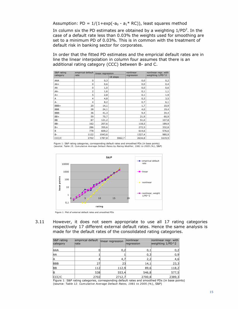
3.10 Figure 1 shows the empirical default rates for all 17 S&P rating categories (RC) and the resulting PDs using exponential smoothing.

Column three and four: linear regression after taking the logarithm Assumption: PD = exp(a0 + a1* RC), least squares method

Column five and six: nonlinear regression

8 Cf. http://www2.standardandpoors.com/spf/pdf/fixedincome/AnnualDefaultStudy_2005.pdf.

15

Assumption: PD = 1/(1+exp(-a0 - a1* RC)), least squares method

In column six the PD estimates are obtained by a weighting 1/PD2. In the case of a default rate less than 0.03% the weights used for smoothing are set to a minimum PD of 0.03%. This is in common with the treatment of default risk in banking sector for corporates.

In order that the fitted PD estimates and the empricial default rates are in line the linear interpolation in column four assumes that there is an additional rating category (CCC) between B- and C.

linear regression S&P rating category

empirical default rate

18 steps

nonlinear regression

nonlinear regr. with weighting 1/PD^2

AAA 0 0,3 0,0 0,2

AA+ 0 0,6 0,0 0,4

AA 0 1,0 0,0 0,6

AA- 2 1,6 0,1 1,1

A+ 5 2,8 0,1 1,9

A 4 4,8 0,3 3,5

A- 4 8,2 0,7 6,1

BBB+ 20 14,1 1,7 10,9

BBB 28 24,1 4,0 19,4

BBB- 36 41,3 9,4 34,4

BB+ 59 70,7 21,9 60,9

BB 87 121,2 51,0 107,8

BB- 162 207,6 118,5 189,9

B+ 286 355,6 272,5 332,8

B 778 609,2 614,6 576,6

B- 1122 1043,6 1327,4 980,9

CCC/C 2702 1787,8 3062,7 2634,8 1619,9 Figure 1: S&P rating categories, corresponding default rates and smoothed PDs (in base points) (source: Table 15. Cumulative Average Default Rates by Rating Modifier, 1981 to 2005 (%), S&P)

S&P

0,1

1

10

100

1000

10000

0 5 10 15 20

rating

base

poin

ts

empirical defaultrate

linear

nonlinear

nonlinear, weight1/PD^2

Figure 1: Plot of external default rates and smoothed PDs

3.11 However, it does not seem appropriate to use all 17 rating categories respectively 17 different external default rates. Hence the same analysis is made for the default rates of the consolidated rating categories.

linear regression S&P rating category

empirical default rate

nonlinear regression

nonlinear regr. with weighting 1/PD^2

AAA 0 0,2 0,1 0,2

AA 1 1 0,3 0,9

A 4 4,7 2,2 4,6

BBB 27 23 14,1 23,3

BB 112 112,9 89,6 118,2

B 538 553,4 546,8 577,5

CCC/C 2702 2712,7 2700,8 2389,3Figure 1: S&P rating categories, corresponding default rates and smoothed PDs (in base points) (source: Table 12. Cumulative Average Default Rates, 1981 to 2005 (%), S&P)

16

3.12 The default rates published by S&P are calculated on a data base that includes also the issuers in the rating category “NR”. These are issuers that had ratings withdrawn. A conservative approach for estimating PDs by external default rates is to eliminate these issuers from the data and recalculate the default rates. These recalculated rates are, in general, greater than those of the conventional default rate calculation. The behaviour of the default rates is nearly similar.

3.13 Figure 4 shows the results for the N.R.-removed default rates

linear regression S&P rating category

empirical default rate

nonlinear regression

nonlinear regr. With weighting 1/PD^2

AAA 0 0,2 0,0 0,2

AA 1 0,9 0,3 0,9

A 4 4,7 2,0 4,6

BBB 27 23,8 13,7 24,2

BB 120 119,9 92,7 126,3

B 591 603,9 600,9 633,5

CCC/C 3041 3040,7 3039,6 2633,5Figure 1: S&P rating categories, corresponding default rates and smoothed PDs (in base points) (source: Table 13. N.R.-Removed Cumulative Average Default Rates, 1981 to 2005 (%), S&P)

S&P (without NR)

0,1

1

10

100

1000

10000

0 2 4 6 8

rating

base

po

ints

empirical defaultrate

linear

nonlinear

nonlinear, weight1/PD^2

Figure 1: Plot of external default rates and smoothed PDs

Moody’s

3.14 Identical calculations were made for the default rates published by Moody’s:

17

Moody’s rating category

empirical default rate

linear regression

nonlinear regression

nonlinear regr. with weighting 1/PD^2

Aaa 0 0,1 0,0 0,0

Aa1 0 0,2 0,0 0,1

Aa2 0 0,4 0,1 0,1

Aa3 2 0,7 0,2 0,2

A1 0 1,4 0,4 0,5

A2 3 2,5 0,8 1,0

A3 4 4,6 1,7 2,1

Baa1 16 8,6 3,5 4,4

Baa2 16 15,8 7,4 9,1

Baa3 33 29,1 15,3 18,7

Ba1 75 53,7 31,9 38,6

Ba2 78 99,0 66,1 79,4

Ba3 207 182,6 136,7 162,6

B1 322 336,7 280,4 330,2

B2 546 620,8 566,6 658,8

B3 1046 1144,5 1111,7 1271,5

Caa-C 2098 2110,2 2066,1 2312,9Figure 1: Moody’s rating categories, corresponding default rates and smoothed PDs (in base points) (source: Exhibit 36 - Average Cumulative Issuer-Weighted Corporate Default Rates by Alphanumeric Rating, 1983-2005, Moody’s)

Moody`s

0,01

0,1

1

10

100

1000

10000

0 5 10 15 20

rating

base

poin

ts

empirical defaultrate

linear

nonlinear

nonlinear, weight1/PD^2

Figure 1: Plot of Moody’s external default rates and smoothed PDs

3.15 Again the linear regression fits well. As mentioned above, the use of 17 different rating categories is too detailed for the standard formula. The results for the whole letter ratings for the identical time are listed below.

Moody's rating category

empirical default rate linear regression

nonlinear regression

Nonlinear regr. with weighting 1/PD^2

Aaa 0 0 0 0

Aa 1 1 2 1

A 2 4 7 3

Baa 21 20 31 17

Ba 131 99 134 97

B 569 501 566 526

Caa-C 2098 2534 2099 2392 Figure 1: Moody’s rating categories, corresponding default rates and smoothed PDs (in base points) (source: Exhibit 35 - Average Issuer-Weighted Corporate Default Rates by Whole Letter Rating, 1983-2005, Moody’s)

18

Figure 1: Plot of Moody’s external default rates and smoothed PDs

3.16 Moody’s illustrates that default rates are calculated on a data base where the issuers whose ratings are withdrawn are excluded “… to account for survivorship bias”. Nevertheless, it is not totally clear whether all these issuers are excluded or just a part of them. The published formula used for calculating the default rates doesn’t respond to that question completing.

Aggregation S&P and Moody’s

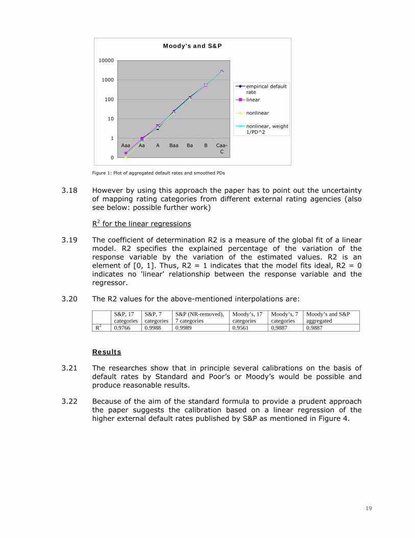
3.17 Under the assumption that the whole letter rating categories by Moody’s are comparable with the compressed rating categories by S&P it would be also possible to aggregate the default rates homogeneous. The results are shown below.

Moodys S&P rating

category default

rate rating

category default

rate aggregated default rate

linear regression

Nonlinear regression

nonlinear regr. with weighting

1/PD^2

Aaa 0 AAA 0 0 0 0 0

Aa 1 AA 1 1 1 1 1

A 2 A 4 3 4 4 4

Baa 21 BBB 27 24 22 20 21

Ba 131 BB 120 125 110 111 115

B 569 B 591 580 555 586 595

Caa-C 2098 CCC/C 3041 2570 2797 2569 2555 Figure 1: Moody’s and S&P rating categories, corresponding default rates, aggregated default rates and smoothed PDs (in base points)

19

Moody's and S&P

0

1

10

100

1000

10000

Aaa Aa A Baa Ba B Caa-C

empirical defaultrate

linear

nonlinear

nonlinear, weight1/PD^2

Figure 1: Plot of aggregated default rates and smoothed PDs

3.18 However by using this approach the paper has to point out the uncertainty of mapping rating categories from different external rating agencies (also see below: possible further work)

R2 for the linear regressions

3.19 The coefficient of determination R2 is a measure of the global fit of a linear model. R2 specifies the explained percentage of the variation of the response variable by the variation of the estimated values. R2 is an element of [0, 1]. Thus, R2 = 1 indicates that the model fits ideal, R2 = 0 indicates no 'linear' relationship between the response variable and the regressor.

3.20 The R2 values for the above-mentioned interpolations are:

S&P, 17 categories

S&P, 7 categories

S&P (NR-removed), 7 categories

Moody’s, 17 categories

Moody’s, 7 categories

Moody’s and S&P aggregated

R2 0.9766 0.9988 0.9989 0.9561 0,9887 0.9887

Results

3.21 The researches show that in principle several calibrations on the basis of default rates by Standard and Poor’s or Moody’s would be possible and produce reasonable results.

3.22 Because of the aim of the standard formula to provide a prudent approach the paper suggests the calibration based on a linear regression of the higher external default rates published by S&P as mentioned in Figure 4.

20

PD estimate S&P rating category

credit quality step

AAA 0,2

AA 1 1

A 2 5

BBB 3 24

BB 4 120

B 5 604

CCC/C 6 3041

Figure 1: Calibration proposal

A) Correlation

3.23 CP 20 suggests in § 5.212 to use a base correlation of 0.5 for the theoretical case of infinitely many issuers and to adjust this correlation with a correlation depending on the Herfindahl Index.

The Herfindahl index

3.24 The Herfindahl index is a commonly used ratio to measure concentrations. The benefit of the Herfindahl index is that it gives a weight depending on the risk exposure to the counterparties.

Example: The risk exposure is divided among five counterparties.

A: The total reinsurance exposure is divided equally among the five counterparties.

H = 5 * (0.2)2 = 0.2

B: The exposure to counterparty 1 represents 80% of the total exposure. The esposure to counterparties 2 to 5 is consistently 5%.

H = (0.8)2 + 4 * (0.05)2 = 0.65

3.25 If n denotes the number of counterparties in the portfolio, the Herfindahl index ranges from 1/n to 1. For a single counterparty (n=1), the Herfindahl index is equal to 1. If the fraction of the reinsurance exposure is identical to all counterparties, the Herfindahl index is equal to 1/n. So a small Herfindahl index indicates a well diversified portfolio.

Base Correlation

3.26 The Basel II accord in Banking sector models the correlation as an inverse function of the PD between an upper limit of 24% and a lower limit of 12% for well diversified loan portfolios.

3.27 Reinsurers tend to be quite large and, because of same business, higher correlated as randomly selected companies in a diversified portfolio. Due to this fact it would be not appropriate to use the Basel II correlations.

3.28 The paper causes the calibration of the base correlation on a study of KMV (KMV, An Empirical Assessment of Asset Correlation Models, 20019). This

9 Cf. http://www.moodyskmv.com/research/files/wp/emp_assesment.pdf

21

study uses weekly returns of more than 27,000 firms diversely distributed in more than 40 countries and 61 industries as data base to validate the out-of-sample performance of different asset correlation models (among others historical models, average models, single factor models).

3.29 The data base was divided in several sub-samples. The first of these sub-samples includes 1000 companies with the smallest numbers of missing weekly returns. Given the certainty that larger and more stable firms tend to have more observations, the results on this sub-sample can be viewed as primarily for large firms like reinsurers.

3.30 Figure 14 shows that 95% of the companies have an asset correlation coefficient lower than around 45%. The historical model offers the highest forecasted correlations with about 87%. KMV applies an upper limit of 65%.

Figure 1: forecasted correlations (source: KMV)

3.31 Additional out-of-sample analysis in the study demonstrated that the forecast performance of e.g. the historical model was quite well.

Figure 2: forecast performance (source: KMV)

3.32 Because of the already in CP20 mentioned circumstance that insurers tend to have very few selected counterparties for risk mitigation and the above-quoted study of KMV the paper propose a conservative base correlation of 50% added by the product of the base correlation and the Herfindahl index.

22

4. Section 4

Concentration risk

Introduction

4.1 Market risk concentrations present an additional risk to an insurer because of:

additional volatility that exists in concentrated asset portfolios; and

the additional risk of partial or total permanent losses of value due to the default of an issuer

4.2 For the sake of simplicity and consistency, the definition of market risk concentrations is restricted to the risk regarding the accumulation of exposures with the same counterparty. It does not include other types of concentrations (e.g. geographical area, industry sector etc.)

Specification

4.3 The calculation is performed in four steps: (a) net exposure, (b) excess exposure, (c) risk concentration charge per ‘name’, (d) aggregation.

(a) The net exposure Ei to a single counterparty i is calculated as the sum of the exposures across asset classes k:

∑=

=2

1kk,ii EADE

(b) The excess exposure is calculated as:

⎭⎬⎫

⎩⎨⎧

−= CTAssets

EXS

xl

ii ;0max

,

where the concentration threshold CT, depending on the rating of counterparty i, is set as follows:10

10 Note that a concentration threshold of e.g. 5% means that at most 20 of the largest risk concentrations need to be considered for the purposes of this module.

23

ratingi CT

AA-AAA 5%

A 5%

BBB 3%

BB or lower 3%

(c) The risk concentration charge per ‘name’ i is calculated as:

)( 10 iixli XSggXSAssetsConc •+••= ,

where XSi is expressed with reference to the unit (i.e. an excess of exposure i above the threshold of 8%, delivers XSi = 0.08) and where the parameters g0 and g1, depending on the credit rating of the counterparty, are determined as follows:

ratingi Credit Quality Step G0 G1

AAA

AA 1 0.184 0.040

A 2 0.268 -0.016

BBB 3 0.386 -0.042

BB or lower, unrated

4 – 6, - 0.923 -0.431

(d) The total capital requirement for market risk concentrations is determined assuming independence between the requirements for each counterparty i:

∑=i

iconc ConcMkt 2

4.4 Risk exposures from assets need to be grouped with respect to counterparties and with respect to the two asset classes ‘equity’ and ‘fixed income’.

EADi,k = The net exposure at default to counterparty i in asset class k

Assetsxl = The amount of total assets excluding those where the policyholder bears the investment risk

ratingi = The external rating of the counterparty i

4.5 All entities which belong to the same group should be considered as a single counterparty for the purposes of this module.

24

4.6 The asset class index k takes the two values ‘equity’ and ‘fixed income’. For the purposes of QIS3, real estate holdings and exposure to property funds are not to be included. All other financial assets are to be classified as either ‘fixed income’ (if senior debt) or ‘equity’ (otherwise). In case of hybrid instruments (e.g. junior debt, mezzanine CDO tranches, …) or in case of doubt the exposure is to be treated as equity.

4.7 Financial derivatives on equity and defaultable bonds should be properly attributed (via their ‘delta’) to these two classes. I.e., an equity put option reduces the equity exposure to the underlying ‘name’ and a single-name CDS (‘protection bought’) reduces the fixed-income exposure to the underlying ‘name’. The exposure to the default of the counterparty of the option or the CDS is not treated in this module, but in the counterparty default risk module.

4.8 Exposures via investment funds or such entities whose activity is mainly the holding and management of an insurer’s own investment need to be considered on a look-through basis. The same holds for CDO tranches and similar investments embedded in ‘structured products’.

Calibration

1st. step.- The starting point is the design of a well-diversified portfolio of investments in individual names with the following characteristics:

(a) The portfolio has a mix, representative of EU average insurers’

portfolios of investments in bonds and equities. The mix proposed is 70% - 30% corresponding bonds – equities respectively (see figure 11A, page 12, Financial Stability Report Conglomerates 2005-2006).

(b) Within each of these two groups, a sector-distribution of investments is built, also according to an EU expected average, as follows:

i. Investment in bonds: We have assumed that 25 % of bonds-portfolio is invested in risk-free bonds, and the rest (75 %) is invested in different sectors and ratings as described below.

ii. Investment in equities: To the extent that this exercise assumes as starting point a well-diversified portfolio, consequently it should replicate some equity index sufficiently representative and well-known. The selected index is Eurostoxx 50, and the period used to record data on prices of each of its element, ranges from 1993-january-11st until 2006-november-30th. The length of this period guarantees sufficient historical data to derive VaR 99.5% with a high degree of reliability. Some elements of the selected index have been removed, since their records of data prices are only

25

available for a significantly shorter period than that above mentioned11.

Description of bonds-portfolio

4.9 In order to avoid the effect of the change in Macaulay Duration (as the life of the bond expires) and the renewal of the investment12, and what is more important, to reflect the whole risk belonging to each sector/rating it was decided:

1) Bonds used in the computation are notional bonds, all of them issued at 5% rate and pending 5 years to maturity. At any moment of the simulation each bond maintain these features (which could be accepted as representative average features of the bonds existing in insurance portfolios)

2) To capture and summarize market information about each sector/rating, notional bonds described in point 1) are valued with Bloomberg corporate yield curves, according the corresponding sector/rating. The following table lists these yield curves:

INTEREST RATES DATA

1 F888 EUR BANK AAA 2 F462 INDS AA+ 3 F890 BANK AA 4 F580 UTIL AA 5 F892 BANK A 6 F583 UTIL A 7 F465 INDUS A 8 F898 BANK BBB 9 F625 TELEF A

10 F468 INDUS BBB 11 F469 INDUS BBB- 12 F682 TELEF BBB+ 13 F470 INDUS BB

11 As part of the initial steps of calibration exercise of concentration risk, a complete set of tentative checking-tests was carried out to optimize the design of the method. The outputs of these preliminary calculations may be summarized as follows:

- Dealing with concentration risk requires obviously the use, as starting point, of a sufficiently high number of exposures,

- Nevertheless, as important as the number of different exposures is to guarantee that the selected names reflect a variety of behaviours sufficiently disperse, in such a way that almost all existing and possible equities/bonds fall in the range of behaviours considered

- Under the above assumption, increasing the number of names did not have a significant added value (the outputs were rather similar), while the computational burden increased and the analysis of a higher number of names became less transparent.

12 This could be seen quite arbitrary, because we should have to select again another similar bond to substitute the previous one

26

Description of equities portfolio

4.10 To obtain a well-diversified portfolio, after selecting the components of Eurostoxx 50 mentioned above, other additional names have been added to complete all the buckets of the cross-table resulting from, on one dimension rating categories considered, and on the other dimension economic sectors included in this exercise.

Weights for each name in this initial portfolio depend on the following features:

1) When calculating BB concentration risk polynomial: we use names ranged from B to AAA

2) When calculating BBB, A and AA-AAA concentration risk polynomials: we use the names ranged from BBB to AAA with the relevant adjustment in their initial weight

3) Besides, the level or quality of diversification of these two starting portfolios has being checked by calculating their Herfindal index and comparing with their minimum possible value:

∑=

=n

iiwIndexHerfindal

1_

4.11 This table shows in all cases a Herfindal index for each portfolio only 0.005 higher than the minimum possible value, which confirms that the selected portfolios are actually well-diversified.

4.12 Finally, the calibration exercise has calculated the historic 1-year VaR 99.5% of a mixed portfolio (30 % invested in the equities portfolio, and 70 % invested in the bonds portfolio). This measure is calculated twice:

Firstly, taking into account all the names and its corresponding yield curves as listed above:

VaR (99.5 %) = 12.85 %

Secondly, excluding BB names and its corresponding yield curve, as listed above.

VaR (99.5 %) = 10.88 %

In both cases, risk-free bonds are priced with the German sovereign curve.

27

4.13 As one can appreciate, there is sufficient rationale to calibrate firstly BB polynomial using the whole portfolio and afterwards, in a second step, to calibrate BBB, A and AA-AAA polynomial with a less volatile portfolio. 13

2nd step.- Concentrating exposures in the initial portfolio:

4.14 First of all, we have established a bijective correspondence between each equity name and one of the interest rates curves above listed, taking into account its sector / rating. This means that when we concentrate the whole portfolio we concentrate at the same time the investment in the selected equity and its correspondent notional bond.

1. The exercise begins selecting a concrete name with a certain rating, (i.e. a bank rated AAA) and its correspondent notional bond (Banks AAA). Then, we increase in steps of 1 per cent its total weight in respect of the whole portfolio, obviously reducing simultaneously the participation of the rest of counterparties (to isolate purely the effect of concentration on the selected name).14

2. Increases of concentration levels range from the starting weight up to the starting weight plus 71%, (as above mentioned, using 1% steps). For each level of concentration, we calculate the difference between the historic 1-year VaR 99.5% of the starting portfolio and historic 1-year VaR 99.5% of the resulting concentrated portfolio, and this difference is considered a raw proxy of an eventual concentration charge (it is called Variation VaR.)

3. Points of raw-concentrations charges obtained in the successive increases of concentration for each name are drawn, interpolating a 2nd degree polynomial, and then deriving the parameters g0 and g1

(note that according the formula contained in paragraph 5.199 of CEIOPS CP 20, g0 = f0* RW(rating), and g1= f1*RW(rating) ). Thus, for each level of rating i we wil have:

12

0 gXSAssetsgXSAssetsConc ixlixli ••+••=

3rd step.- The same procedure is repeated for names rated AA, A, BBB and BB or worse and different sectors.

4.15 Note that the initial investment in risk-free bonds remains unchanged. Therefore concentration exercise refers to the whole equity portfolio and 75% of the bonds-portfolio.

13 One have to bear in mind that due their high volatility, considering BB curve and BB-B equities increases (in relative terms) the goodness of the rest of names/ratings.

14 Note that equities and bonds are simply added, without applying the weights contained in par. 5.195 of CEIOPS Consultation Paper 20. This minor and technical change is proposed for various reasons, presented for approval during CEIOPS Pillar I WG meeting held in January 10, and having obtained the necessary agreement.

28

4.16 Tables below compare 1-year historical VaR 99’5% for the starting portfolio versus the extreme 1-year historical VaR 99’5% (portfolios with a concentration increase of 71 % above the initial weight). See Table 4.x for calculations including BB & B exposures and Table 4.xx for calculations excluding such exposures.

Table 4.x Calculations including BB & B exposures

Those who

improve Those who decrease

AAA+AA A BBB WORSE

Mean 2,3784% -10,7817% -0,70% -1,44% -6,15% -26,00% Standard Dev 1,1290% 12,6649% 6,1265% 5,9730% 9,1125% 20,1174% N 15 12 7 3 Variation Coef 47,4674% -117,4670%

-870,2377%

-414,3150%

-148,2736%

-77,3748%

Table 4.xx Calculations excluding BB & B exposures

Those who

improve Those who decrease

AAA+AA A BBB

Mean 1,6138% -6,8795% -2,01% -3,25% -7,75% Standard Dev 1,4912% 7,4379% 6,3729% 5,8990% 9,1288% N 15 12 7 Variation Coef 92,3996% -108,1159%

-316,6407%

-181,2757%

-117,7904%

4.17 Once reached this point and analysed the graphs obtained, the

interpolation of a 2nd degree polynomial is carried out taking into account the worst-behaved names are. This criterion is necessary to guarantee the consistency of the calibration exercise with the rationale grounding the standard SCR formula, which focus on stressed scenarios.15

15 Due to its own characteristics, the mean VaR for each group of rating (BB, BBB, A and AA-AAA), tends to smooth the risk of concentration, thus understating the corresponding capital charge.

29

4.18 See in figure 1 the selected lines and the interpolated one for AA-AAA rating (the last one). Each line means the Variation VaR when the portfolio increases the concentration in each equity and its correspondent AA bond.

0 10 20 30 40 50 60 70 80-0.25

-0.2

-0.15

-0.1

-0.05

0

0.05

0.1

data1

data2

data3

data4

Figure 1

4.19 Figure 2 plots the selected lines and the interpolated one for A rating, with

similar meaning and methodology as the previous graph.

0 10 20 30 40 50 60 70 80-0.16

-0.14

-0.12

-0.1

-0.08

-0.06

-0.04

-0.02

0

0.02

data1

data2

data3

Figure 2

30

4.20 Figure 3 depicts the selected lines and the interpolated one for BBB rating, following the same rationale and presentation as above

0 10 20 30 40 50 60 70 80-0.25

-0.2

-0.15

-0.1

-0.05

0

0.05

0.1

data1

data2

data3

Figure 3

4.21 Figure 4 contains the lines and the interpolated one for BB or worse rating.

0 10 20 30 40 50 60 70 80-0.5

-0.4

-0.3

-0.2

-0.1

0

0.1

0.2

Figure 4

4.22 Finally, g1 and g2 parameters of each polynomial for each rating are estimated using a conventional minimum squares method and included a judgmental adjustment to consider:

- the method has focused on non-systemic volatility risk (the first type of risk captured in this submodule), assuming that due to the long period analysed, outputs reflect partially the second source of risk which should be captured in concentration submodule (risks of losses

31

due to a default in the concentrated exposure). Nevertheless, the method may not achieve a full reflection of this second risk.

- after QIS3 some adjustments in the coefficients resulting from this calibration may be necessary to coordinate on the one hand the correlation implicit in this method among concentration risk and other market risks (equity, interest rate risk and spread risk), and on the other hand the correlation coefficients used in QIS3.

Results

4.23 Concentration risk model for each group of rating i:

Conci = Assets * XSi * ( g1 + g2 * XSi )

Where

iXS = Excess exposure at each group of rating i

⎭⎬⎫

⎩⎨⎧

−= ixl

ii ratinggroupThresholdionConcentrat

AssetsratinggroupExposure

XS _____

;0max

Assets * XSi = excess of exposure i above the threshold, expressed in units instead of percentage

g1 + g2 * XSi = the progressive capital charge obtained as result of the calibration exercise

4.24 As one can see, the formula has been calibrated for different thresholds

depending on each group of rating. These thresholds are listed in the following table:

Group of rating Threshold AA-AAA 0.05

A 0.05 BBB 0.03

BB-worse-unrated 0.03

4.25 The existence of different thresholds grounds on the fact that capital charges obtained according the calibrated parameters for buckets AAA-AA and A are not material for concentrations between 3-5%.

4.26 The final coefficients for each group of rating are the following ones:

32

Table 4 Concentration capital charges for each group of rating.

Final result of calibration excercise g1 g2

BB 0,9227 -0,4314 BBB 0,3862 -0,0416 A 0,2684 -0,0163

AA y AAA 0,1840 0,0401

4.27 Figure 5 shows the estimated polynomials for each group of rating

Figure 5

0

0,05

0,1

0,15

0,2

0,25

0,3

0,35

0,4

0,00

0,03

0,06

0,09

0,12

0,15

0,18

0,21

0,24

0,27

0,30

0,33

0,36

0,39

0,42

0,45

0,48

XS i

Con

c i

y BB y BBB y A y AAA

33

5. Section 5

Examples

CRD comparison

5.1 Many assets held by insurers are relatively liquid and thus incomparable to the credit risks held by banks in the banking book. This would imply that the trading book regulation is the proper counterpart for some assets also in terms of the level of capital requirements. On the other hand, many assets are held to maturity by insurers. This would imply that the capital requirements should by somewhat consistent with the banking book regulations. In practice, the liquidity of assets held by insurers will be somewhere between the illiquid loans held by banks and the assets held by banks for the purpose of trading. To start off, this section compares the spread risk module with the foundation IRB approach

5.2 The foundation IRB allows banks to base the estimation of probability of default (PD) on internal ratings. The risk weight associated with a PD is given by a “risk-weight function” that is motivated by the so-called Vasicek-distribution. The risk weight also depends on the loss given default (LGD), maturity (M) and exposure at default (EAD). In the foundation approach banks are allowed to provide their own estimate of PD. Other parameters that enter the risk-weight functions are prescribed by the supervisor, differing among numerous sub- and sub-subcategories.

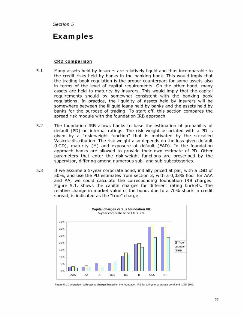
5.3 If we assume a 5-year corporate bond, initially priced at par, with a LGD of 50%, and use the PD estimates from section 3, with a 0,03% floor for AAA and AA, we could calculate the corresponding foundation IRB charges. Figure 5.1. shows the capital charges for different rating buckets. The relative change in market value of the bond, due to a 70% shock in credit spread, is indicated as the “true” charge.

Figure 5.1.Comparison with capital charges based on the foundation IRB for a 5-year corporate bond and LGD 50%.

Capital charges versus foundation IRB 5-year corporate bond LGD 50%

0%

5%

10%

15%

20%

25%

30%

35%

AAA AA A BBB BB B CCC NR

"True"LinearIRB

34

Possible future work

5.4 Further work is needed:

sensitivity analysis on the LGD, maturity and other assumptions.

Extent to other CRD approaches (standardised approach etc.)