NATURAL DISASTERS AND GROWTH: EVIDENCE USING A WIDE PANEL OF COUNTRIES

CHRISTIAN R. JARAMILLO H.1

Abstract Large natural disasters (LNDs) are ubiquitous phenomena with potentially large impacts on the infrastructure and population of countries, and on their economic activity in general. I examine the occurrence pattern of several types of disasters on a panel of 113 countries and its relationship with economic growth using data ranging from 1960 to 1996. The disasters are earthquakes, floods, slides, volcano eruptions, tsunamis, wind storms, wild fires and extreme temperatures. The country sample is partitioned in two ways: small, medium and large population; and low, medium and high income. The results suggest a heterogeneous pattern of short and long-term impact of LNDs, depending on the per capita GDP, the size of the countries studied and the type of LND. Overall, and contrary to previous research, LNDs appear to have persistent effects on the rate of GDP growth in the period between 1960 and 1996. These effects range from a decrease of 0.9% to an increase of 0.6%, depending on the type of disaster.

Keywords: Natural disasters, catastrophes, growth, foreign aid, panel data.

JEL Classification: O11, O19, Q54.

1 Assistant Professor of Economics, Universidad de los Andes. Address: Cra 1 #18A-10, Facultad de Economía, Bogotá, Colombia. Tel (+571) 339 4949 ext. 2439. E-mail: chjarami@uniandes.edu.co.

CEDE

DOCUMENTO CEDE 2007-14 ISSN 1657-7191 (Edición Electrónica) JULIO DE 2007

2

DESASTRES NATURALES Y CRECIMIENTO: EVIDENCIA DE UN PANEL DE PAÍSES

Resumen

Las catástrofes naturales son fenómenos frecuentes con efectos potencialmente grandes sobre la infraestructura y la población de los países, y sobre su actividad económica en general. Este trabajo explora los patrones de ocurrencia de varios tipos de desastres en un panel de 113 países, y su relación con el crecimiento económico en el periodo 1960-1996. Los desastres considerados son terremotos, inundaciones, avalanchas, erupciones volcánicas, tsunamis, huracanes y tormentas de viento, incendios forestales, y temperaturas extremas. La muestra de países se divide de dos maneras: países con poblaciones pequeñas, medianas y grandes; y países de ingresos per cápita bajos, medios y altos. Los resultados sugieren patrones heterogéneos de efectos de corto y largo plazo según el tipo de desastre, la población del país y su nivel de ingreso per cápita. En general, y en contraste con la evidencia previa, las catástrofes tienen efectos persistentes sobre la tasa de crecimiento del PIB per cápita en el periodo de análisis. Estos efectos oscilan entre una disminución de 0.9% y un aumento de 0.6% en el crecimiento de largo plazo, según el tipo de desastre.

Palabras clave: Desastres naturales, catástrofes, crecimiento, ayuda externa,

datos en panel.

Clasificación JEL: O11, O19, Q54.

3

1. Introduction

Large natural disasters (LNDs for short) are ubiquitous events with potentially large impact

on the infrastructure and population of countries, and on their economic activity in general.

While case studies of disasters abound and there are some small-panel studies,2 I am not

aware of any work that uses time-series data from a large number of countries to examine

the importance of this impact.

In this paper, I explore the relationship between disasters and growth using panel data on

recorded disaster events and macroeconomic variables of 113 countries over a 36-year

span. I test for the effect of a disaster on current and next-year GDP growth (short-run

effects). I also test for cumulative effects of disasters, which are interpreted as long-run

effects, and compare the results to previous research that suggests small to non-existing

long-term effects.

The data is a panel from different sources, including disaster measures and national

accounts for a wide sample of countries. The data on disasters comes from EM-DAT: The

OFDA/CRED International Disaster Database. It contains records of estimated damages,

people killed, injured, homeless and affected for occurrences of natural, technological and

political disasters, as well as dates of occurrence and the countries affected. The data are

a compilation from different sources, among them the UN, OFDA, reinsurance firms and

several NGOs and humanitarian institutions, and it includes events starting 1900 through

the present.

The time series data on macroeconomic variables comes from several sources. Whenever

available, I use the Penn World Tables 6.0. These contain data from 1950-1998, albeit

most countries start reporting in 1960. This period seems to coincide with the more reliable

data in the EM-DAT database. Foreign aid data is from the OECD’s DAC/GEO database.

2 See Auffret (2003a), Albala-Bertrand (1993).

4

The next section presents the theoretical framework. Section 3 describes the data in detail,

emphasizing various aspects that require special attention. In section 4 I present the

empirical specifications for the econometric analysis and the estimation results. Section 5

concludes.

2. Theory and Evidence of the economic Impact of Disasters

How may a catastrophe influence a country’s economy? Macroeconomic theory allows for

several types of possible impacts of a LND. First, a disaster destroys capital stock and

labor. Insofar as this raises the rates of return to these factors, one should expect

increased investment activity in the economy. This should be an effect of limited duration,

and it should concern the level of GDP rather than its long-term growth path. A priori, this

effect should be negative on the level of GDP. Nevertheless, because capital losses due to

LNDs do not show up in national accounting but the surge in investment does, one might

find a positive net effect in the recorded data. In this respect, the existing literature is

based on individual cases, and it argues that substitution in production limits the size of the

negative effects (Horwich 2000). For a sample of 28 disasters that took place between

1960 and 1979 in 26 developing countries, Albala-Bertrand (1993, Ch. 4) finds that GDP

level does not suffer after a disaster and inflation does not rise. Auffret (2003a), in

contrast, finds that disasters lead to a fall in output in a sample of 16 countries in latin

America and the Caribbean for the period 1970-1999.3

A second and potentially more important avenue for LND impact has to do with per capita

GDP growth rather than its level. One could think of a number of scenarios, all involving

market imperfections, where the post-LND growth rates are different from the pre-disaster

ones. Unfortunately, the literature on GDP growth suggests that one must take some

subjective stand on what one views as the long run to address this question, since a 3 See also Raddatz (2005, no effects), Crowards (1999, short-term effects, as cited in Charvériat 2000). Charvériat (2000) and Albala-Bertrand (1993) provide and extensive discussions on the theory and evidence of the economic impact of natural disasters. Also, the Economic Comission for Latin America and the Caribbean has numerous case studies and policy analyses on disaster prevention, preparedness and relief (http://www.eclac.cl).

5

definitive empirical answer cannot be obtained from a finite time series of data (Christiano

and Eichenbaum 1989). What does the evidence say about these long-run effects? Albala-

Bertrand reports small positive effects on GDP growth thanks to large increases in

construction and smaller ones in agricultural output. The trade deficit increases, however.

Whether these increases are persistent is not clear.

In view of the loss accounting issue, a country's reaction to LNDs would perhaps be best

judged on the basis of its investment activity, both in absolute levels and as a share of its

GDP. This investment must be financed either through current consumption cuts (private

or governmental) in the case of a credit-constrained economy, or through borrowing (which

entails a smaller but permanent decrease in consumption) and foreign investment. Thus,

the country will substitute away from consumption, and this level effect will be smaller but

more persistent if the country's economy has access to international credit. Here the

evidence is sometimes in agreement and sometimes at odds with the predictions, and

different studies contradict each other. Albala-Bertrand (1993) reports that gross fixed-

capital formation tends to increase, financed with a small increase in public deficits and

large inflows of capital. Auffret (2003a) adds a decrease in private and (inconsistent with

the larger public deficits) public consumption growth, and confirms also the deterioration of

the current account. Crowards (1999) reports sharp increases in GDP the years after the

disaster due to investment.

Of course, this is not an exhaustive list of interesting economic questions related to LNDs.4

Institutions matter in the face of catastrophe risk. The depth of insurance markets plays a

fundamental role (Auffret 2003b, Charvériat 2000). So do informal insurance mechanisms

(Fafchamps and Lund 2003, Jalan and Ravallion 2001), and more generally the

households’ strategies to cope with risk, which may help to explain the persistent effects

on growth through human capital investment (Rosenzweig and Stark 1989, Jensen 2000,

Jacoby and Skoufias 1997). The effectiveness of foreign aid as a tool to mitigate disaster

4 Their impact on aggregate consumption patterns and on trade, or the institutional aspects of disaster responses, are examples of macroeconomic issues with no clear-cut theoretical predictions. There’s also a wide range on microeconomic questions: sustitution in production, formal and informal insurance and household impact, to name a few.

6

impact depends on the quality of policies and institutions (Burnside and Dollar 2000,

Easterly 2003), albeit it is not clear that its true aim is indeed this (Alesina and Dollar

1998).

Finally, asymmetric information and institutional factors may be a source of persistence in

the effects of LNDs. For instance, the modes of investment that take place a country, in

particular the role of foreign direct investment (FDI), may be affected by a disaster either

directly, or indirectly through the disaster impact on other economic variables and

government policies. Or the foreign aid flows may alter the institutions prevalent in the

affected countries (Weder 2000). There's no unambiguous prediction regarding these

matters, as it is unclear how the aftermath of a LND or the attention a country may get

from it will affect –if at all– the determinants of the choice of FDI versus other types of

capital flows or the quality of institutions.

Ultimately, none of the answers in the macroeconomic literature predicts long-term growth

effects of LNDs except in extreme market failure cases. The focus of this paper is to

determine whether the evidence shows robust long-term effects in spite of macroeconomic

predictions.

3. Data The data for the yearly panel of countries comes from several sources. I use country

macroeconomic time series from the Penn World Tables 6.0 (PWT).5 International data on

official foreign aid is self-reported by the members of Development Assistance Commitee

(DAC) of the Organisation for Economic Cooperation and Development (OECD). It is

available in the DAC/GEO database of Geographic Distribution of Financial Flows to Aid

Recipients, 1960-1998, included in the OECD publication International Development

5 The PWT can be found at the Center for International Comparisons, University of Pennsylvania. http://pwt.econ.upenn.edu/

7

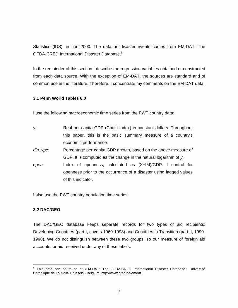
Statistics (IDS), edition 2000. The data on disaster events comes from EM-DAT: The

OFDA-CRED International Disaster Database.6

In the remainder of this section I describe the regression variables obtained or constructed

from each data source. With the exception of EM-DAT, the sources are standard and of

common use in the literature. Therefore, I concentrate my comments on the EM-DAT data.

3.1 Penn World Tables 6.0 I use the following macroeconomic time series from the PWT country data:

y: Real per-capita GDP (Chain Index) in constant dollars. Throughout

this paper, this is the basic summary measure of a country's

economic performance.

dln_ypc: Percentage per-capita GDP growth, based on the above measure of

GDP. It is computed as the change in the natural logarithm of y.

open: Index of openness, calculated as (X+IM)/GDP. I control for

openness prior to the occurrence of a disaster using lagged values

of this indicator.

I also use the PWT country population time series.

3.2 DAC/GEO The DAC/GEO database keeps separate records for two types of aid recipients:

Developing Countries (part I, covers 1960-1998) and Countries in Transition (part II, 1990-

1998). We do not distinguish between these two groups, so our measure of foreign aid

accounts for aid received under any of these labels:

6 This data can be found at \EM-DAT: The OFDA/CRED International Disaster Database." Université Catholique de Louvain- Brussels - Belgium. http://www.cred.be/emdat.

8

aid: Net total foreign official aid flow to a recipient country in a given year,

expressed as a fraction of its current GDP.

As net total foreign official aid flow, we use the DAC/GEO time series on Total Official Net

flows of aid by recipient. This data is the sum of Official Development Assistance (ODA)

and Other Official Flows (OOF) for part I countries, and of Official Assistance (OA) and

Other Official Flows (OOF) for part II countries. It represents the total net disbursements by

the official sector at large to the recipient country in either case.

While the flows recorded in the DAC/GEO data are only those of OECD origin, they

account for most of the international flows of official foreign aid in any given year from

1960-1998 for part I and 1990-1998 for part II. The countries of origin covered are the DAC

Donor Countries: Australia, Austria, Belgium, Canada, Denmark, Finland, France,

Germany, Ireland, Italy, Japan, Luxembourg, the Netherlands, New Zealand, Norway,

Portugal, Spain, Sweden, Switzerland, the United Kingdom, and the United States.

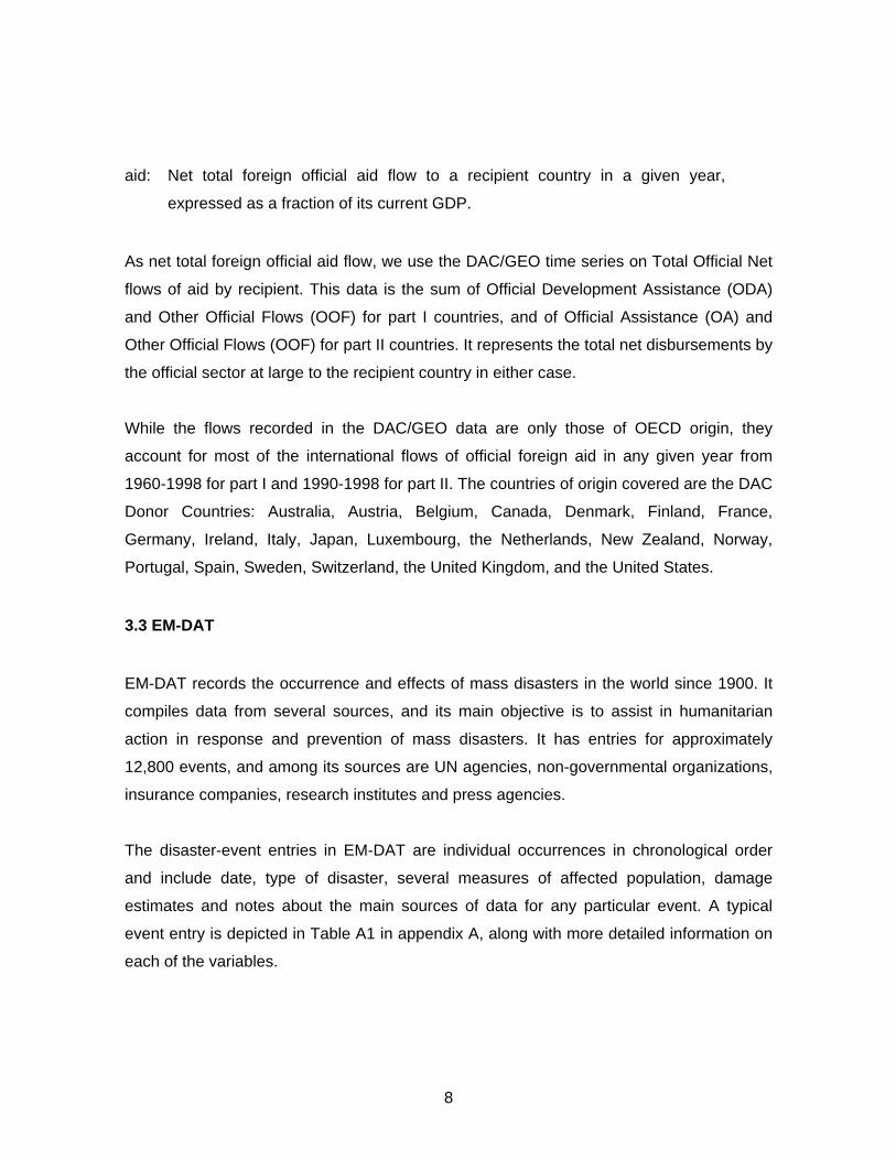
3.3 EM-DAT

EM-DAT records the occurrence and effects of mass disasters in the world since 1900. It

compiles data from several sources, and its main objective is to assist in humanitarian

action in response and prevention of mass disasters. It has entries for approximately

12,800 events, and among its sources are UN agencies, non-governmental organizations,

insurance companies, research institutes and press agencies.

The disaster-event entries in EM-DAT are individual occurrences in chronological order

and include date, type of disaster, several measures of affected population, damage

estimates and notes about the main sources of data for any particular event. A typical

event entry is depicted in Table A1 in appendix A, along with more detailed information on

each of the variables.

9

EM-DAT groups disasters in three broad categories (natural, technological and conflict)

with several types, as listed in Table 1 below. In order for an event to qualify for the

registry, it must satisfy at least one of several minimum requirements concerning the

number of victims and the damage amounts.7

My focus is on events that can be unambiguously interpreted as exogenous. Thus, I

concentrate on natural disasters. Moreover, I consider only those types of natural disasters

that can be viewed as occurring at a point in time, rather than those that build up or

develop through extended periods, so I discard droughts and famines. Finally, due to

endogeneity concerns, I drop insect infestations and epidemics from the sample.

The remaining disaster events are earthquakes, floods, wild fires, wind storms, waves and

surges, extreme temperatures, volcano episodes and slides. Figure 1 shows the

geographic distribution of the disasters in our panel. As one should expect, the amount

and types of disasters that occur vary across regions.

From the data in EM-DAT, I construct four types of measures of disaster impact

normalized by the relevant country “size”. These measures concentrate on the disruptive

effect of a LND rather than its physical dimension:

XXtaff: People affected by XX in a given year as a fraction of the current

country population.

XXkill: People killed by XX in a given year as a fraction of the current

country population.

XXdama: Damages due to XX as a fraction of current GDP.

XXdisd: Number of disasters XX in a given year.

7 See appendix A.

10

where XX may be EQ (earthquake), FL (flood), VC (volcano), SL (slide), WS (windstorm),

WF (wildfire), WA (wave/surge) or XT (extreme temperature). Thus each of these

measures exists for each type of disaster considered. For example, there exist EQdisd,

FLdisd, VCdisd, SLdisd, WSdisd, WFdisd, WAdisd and XTdisd.

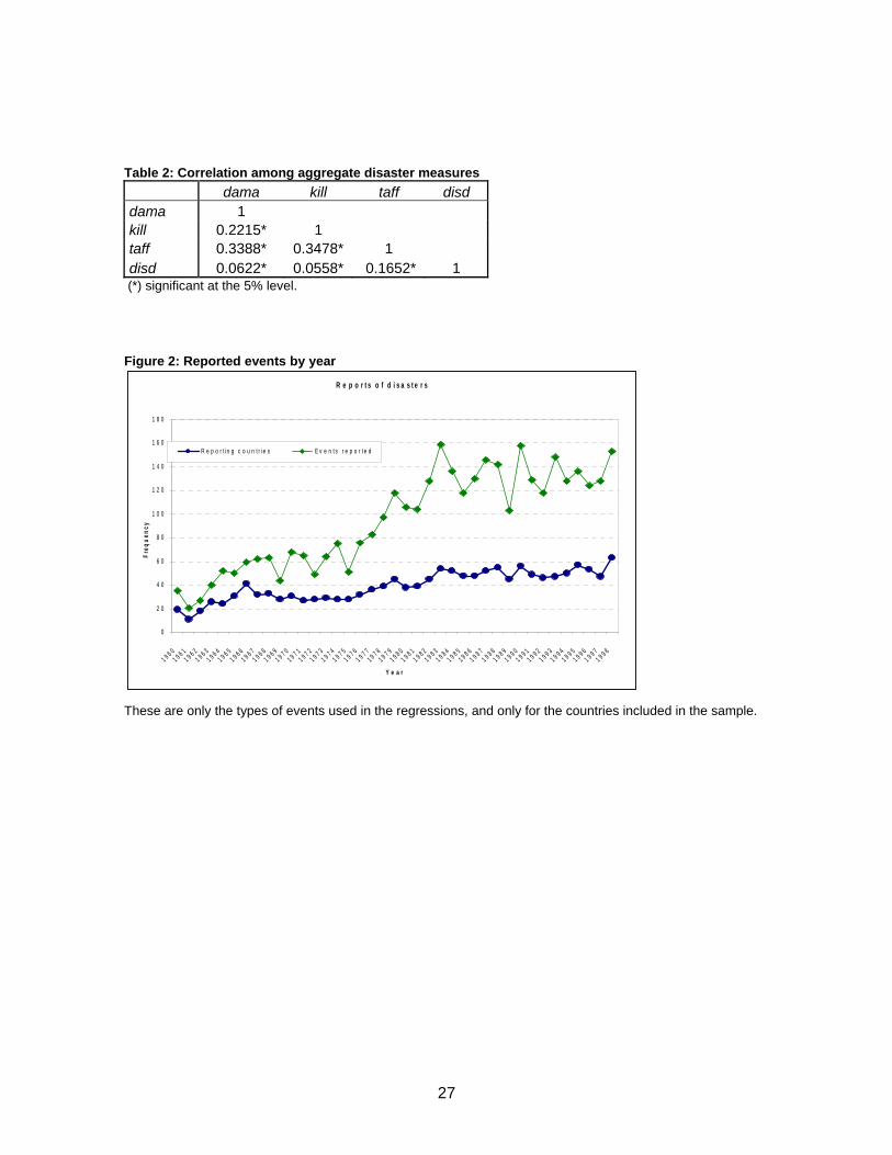
Additionally, I create aggregate measures as the sum over the eight types of disasters for

a given country in a given year. The correlations among these aggregate measures are

reported in Table 2. Not surprisingly, they are positively correlated, although one would

have perhaps expected a higher coefficent.

If no disasters of any type are recorded for a given country in a certain year, disd has a

value of zero for that observation. Whenever disd > 0, there exists a recorded event that

has a non-zero value in at least one among the other three variables. If, for example, kill >

0, the other two variables may be positive, zero or missing.

Suppose dama is missing. There is no way to decide whether this is the result of

misreporting of kill, unavailability of damage estimates, or actual absence of significant

capital losses. My approach to this is straightforward: I replace all missing values of the

three variables taff, kill or dama with zeros. In the cases where missing values are present

but the true value is positive, this approach will generate bias in the estimation. However, it

is likely that in the vast majority of cases missing data values just reflect zero values, or at

most very small ones.

Additionally, I calculate for each type of event and for the aggregate measures the

following cumulative measures of disasters:

cum_taff: Cumulative fraction of people affected, since the first year in the data.

It is calculated as ∑=

=t

iit tafftaffcum0

_τ

τ .

cum_ kill: Cumulative fraction of people killed by LND's since the first year in

the data. This measure and the previous one are based on the

11

country's population in the year the LNDs take place.

∑=

=t

iit killkillcum0

_τ

τ .

cum_dama: Cumulative damages as a fraction of GDP, based on GDP at the

year of LND occurrence. ∑=

=t

iit damadamacum0

_τ

τ .

cum_disd: Cumulative number of disasters since the first year in the data.

∑=

=t

iit disddisdcum0

_τ

τ .

Several concerns besides the missing data must be addressed with EM-DAT. First, it is

difficult to assess and compare the quality of the sources, especially for earlier events. The

multiple sources also account for occasional repeated entries for events, and it is not

always obvious whether two entries with small differences are indeed duplicate. Moreover,

different sources emphasize different data: reinsurance firms likely provide better damage

estimates, but they are based on claims, while UN agents have more encompassing

assessments of damages and affected population. Thus, different data sources have

different strengths (and perhaps systematic biases). Additionally, some data series may be

more informative than others about the true dimension of the event. This is especially the

case if measurement error differs across measures.

Fortunately, this first type of concern, although difficult to address directly, is likely to be of

less importance as the number and scope of international institutions that deal with LNDs

increases. For the time period of our panel, we are confident that this type of noise does

not systematically affect our results.

A second concern, also related to the variety of the sources, is bias over time. The

institutional infrastructure for disaster aid has evolved throughout the 20th century. It is

reasonable to presume that events are more likely to be registered by the authorities in

12

any given country later in the century, and conditional on this, they are also more likely to

be reported to international agencies.

The total number of disasters reported in each year by all countries in the sample is

reported in Figure 2. A log-linear fit with country-specific intercepts shows a yearly

increase of some 1.1% in the period 1960-1998. Since it's reasonable to believe that the

actual number of cataclismic events per year is roughly steady, the increase in events

reported must come, at least in part, from these reporting biases. Another part of these

numbers is certainly a result of increases in population and economic activity: other things

equal, the more people in a country the higher the probability of having 10 deaths in an

earthquake, and the higher the GDP the larger the expected damages from a given

disaster. During the period, a log-linear fit for population growth yields a 2% yearly

increase; and the correlation between the total number of disasters disd and per capita

GDP, plotted in Figure 3, is positive.

Nor is the trend in disaster reports homogeneus across types of disasters. Figure 4 below

shows the number of yearly events reported for each type of disaster.

The largest increases in reports stem thus from floods and windstorms. However, almost

all types of disasters exhibit higher reported frequency over the period. Moreover, these

increases are accompanied with increases in the amounts of damages (as a fraction of

GDP) and affected people (as a fraction of the population, and again especially for floods

and windstorms), albeit not in the amount of killed (Figure 5).

On the other hand, the number of affected and casualties per disaster has remained

roughly steady with a notorious exception: floods, each of which affect more people

nowadays. The average amount of damages has also increased for all disasters,

especially in the last ten years of the sample.8

8 This may be in large part a result of the deepening of insurance markets and the resulting increased incentives to estimate and report damages.

13

One must wonder whether the increased reporting is also a result of a strategic

improvement in record-keeping. It seems that foreign aid as a response to LNDs has risen

in the period of analysis. Could it be that the countries pay more attention to these events

because it pays in terms of getting aid for disaster relief?

The regressions in Table 3 suggest that this is indeed the case: the odds ratio of a country

reporting at least an event increases on average 0.063 each year (column 1).9 Even after

controlling for per capita GDP and population, this effect is correlated strongly with the

world being more generous the year before (columns 3-5).10 However, it may simply be

that reporting improved exogenously and is settling into a new, better standard of

accuracy, as attested by the quadratic trend in columns (6-7). No definitive indictment is

thus possible.

Columns (1-4) in Table 4 show estimates of negative binomial fixed-effects regressions

for the expected number of disaster reports by a country in a year. As before, a quadratic

trend swamps the effect og the lag of world AID, making it difficult to place the blame on

strategic reporting behavior by the countries.

Bias stemming from the failure of a country's authorities to observe and register a disaster

is not likely a grave concern, since an unregistered event is probably one of little impact on

economic activity to begin with. LNDs may be inaccurately measured, but it's difficult that

they go unnoticed. To the extent that it is present, however, this usually downward error in

disd is likely to generate upward bias in our estimates. Thus the trend in reporting, if due to

better record-keeping, is not a major concern provided that one controls with the quadratic

trend.

9 If p is the probability of reporting, the coefficients correspond to the change in the odds ratio p

p−1 due to

a unit increase in the explanatory variable. 10 Fixed effects are used to control for land area, for example, so that together with lnPOP they account for population density.

14

The failure to report an observed disaster to international agencies, on the other hand,

may cause systematic bias and affect the results in unpredictable ways. One can conceive

a number of reasons for some regimes to hide the extent of disasters, or to exaggerate it;

and the correlation of these incentives with our macroeconomic variables is not at all clear.

In this aspect, the variety of sources of the EM-DAT database is an advantage, as it

minimizes the chances that a given event goes completely unrecorded, even if no official

report is filed by the affected country. Partly as a result of this possibility, I believe that any

measurement error problem is likely to be less severe for the variable disd than it is for the

other three measures.11

A third data concern includes endogeneity and timing. I partially address both issues by

concentrating on events that are clearly exogenous (natural disasters) and punctual in

time, i.e. they last a short time (less than a month) and give only short warning.

Nevertheless, this does not completely deal with either issue, as (i) the measured impact

of a given disaster is likely to vary with the economic characteristics of the country itself,

and (ii) the consequences of a disaster need not be punctual or immediate, even if the

disaster itself is. Insofar as this is the case, the disaster counter variable disd is arguably

the least affected by this endogeneity.

This point about the way a LND affects economic activity is complicated by the differences

in the time aggregation of the macroeconomic and disaster time series. Suppose for

instance that there is some delay in part of the impact of earthquakes. If an earthquake

happens in May, its negative impact will be recorded in this year's national accounts. If it

happens in November, most of that impact will show in next year's macroeconomic data.

Suppose instead that the reconstruction activity after the earthquake occurs over a long

period of time. In this case, it is the spurt of investment activity that may be recorded

(positively) in different years depending on the exact month of occurrence. Of course, this

pattern of impact is likely to vary by disaster and by country.

11 Nevertheless, I do exclude from the panel the former communist countries that remain after merging the PWT and EM-DAT, as their incentives for reporting seem particularly dubious. They are Hungary, Romania, Poland and China.

15

While the time pattern of the economic reaction to disasters is precisely what I want to

inspect, this particular aggregation issue is an undesired source of error. For events that

occur randomly throughout the year (like earthquakes), this error is most likely white noise

and causes attenuation bias in some controls of the estimation. In contrast, events that

occur consistently in a given moment of the year (like hurricanes) will bias the results in a

systematic but unpredictable manner.

Finally, even after narrowing the set of events, one might wonder what exactly is

exogenous about them. A country like Colombia, for instance, may not know when an

earthquake will happen, but it certainly knows that it is prone to such disasters. Its

infrastructure is likely to be built using anti-seismic technology, and the actual physical

damages of the eventual earthquake will be smaller. Thus, it is the actual timing of the

disaster that is exogenous, rather than the extent of destruction it causes. Again, this lends

more credibility to the event count variable disd, and it calls for fixed country effects in the

estimation.

4. Estimation

I carry out estimates of two types. First, a naïve cross-section regression of GDP level in

1996 on its 1960 level and the number of disasters in the 36 years in between. In the

second estimation I use a reduced-form panel data specification where I regress the

dependent variable on measures of disaster severity, both instantaneous and cumulative,

and on lags of the instantaneous measures.

4.1 Cross-Section Specification

For a cross section of 104 countries, I regress the level of per capita GDP observed in

1996 on its initial 1960 level and measures of the disasters in the period. To the extent

discussed, the disaster measures are not caused by GDP growth. However, there are

exogenous features of the countries that may cause both higher absolute number of

disasters and growth. Thus I control for the country area (larger countries may have more

16

disasters ceteris paribus) and population growth (or, equivalently, population density). The

regression is then

iiiiii AREAaPOPgrowthaXaGDPaGDP ε++++= lnln1960ln1996ln 2210

where the iX are the cumulative disaster measures in 1996.

I estimate this specification for all countries together, and for two partitions of the sample:

low, medium and high-income countries; and small, medium and large-population

countries.12 Also, I estimate the effects of each type of disaster separately on each

subsample.

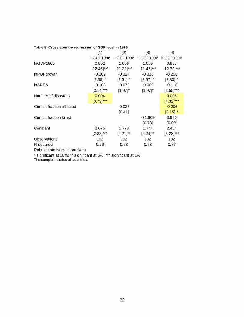
Cross-country regression results are reported in Table 5. The dependent variable is the log

of per-capita GDP in 1996 of a cross section of 102 countries, all those for which GDP,

area and population data is available for both 1960 and 1996. The first dependent variable

is the natural logarithm of per-capita GDP in 1960. The population growth over the period

is given as a percentage change. The disaster measures are the aggregates of all types of

disasters. The estimation is performed by OLS. Columns (1-3) are displayed for

comparison.

In the estimates in column (3), a disaster is related to 0.6% higher per-capita GDP at the

end of the period, significant at the 1% level.13 How large are these effects in practice?

Table 6 below reports the implied change in the 1996 level of GDP if a country increased

its disaster measure by a standard deviation in the corresponding regressions of Table 5.

For instance, the effect of having a standard deviation more disasters would have meant

19.81% higher per capita GDP in 1996. 12 The income subsamples are determined according to the countries’ per capita GDP level in 1960. Similarly, the population subsamples depend on their 1960 population. The countries in each subsample are listed in the Appendix C. 13 It is possible that the effects of disasters over a long period of time have a non-linear component, either because of cumulative aspects of events over several years, or because multiple catastrophic events in a given year are compounded in a non-linear fashion.

17

The usual precaution regarding unobserved variables is required in this analysis. The

assumption that the changes in population and the initial GDP are uncorrelated with the

error terms is precarious at best. Even if population growth is viewed as truly exogenous,

the initial GDP is most certainly correlated with unobserved idiosyncratic country features,

fixed and otherwise. We address this problem in detail later. Still, for the time being a

relationship between LNDs and growth seems likely.

Table 7 is analogous to column (4) in Table 6 and reports implied level effects for each

subsample of countries, using the cross-country specification. Some of the level effects

are large: a 20% increase in the 1996 GDP level corresponds to a yearly increase in

growth rates from 2.0% to 2.3% for 36 years14.

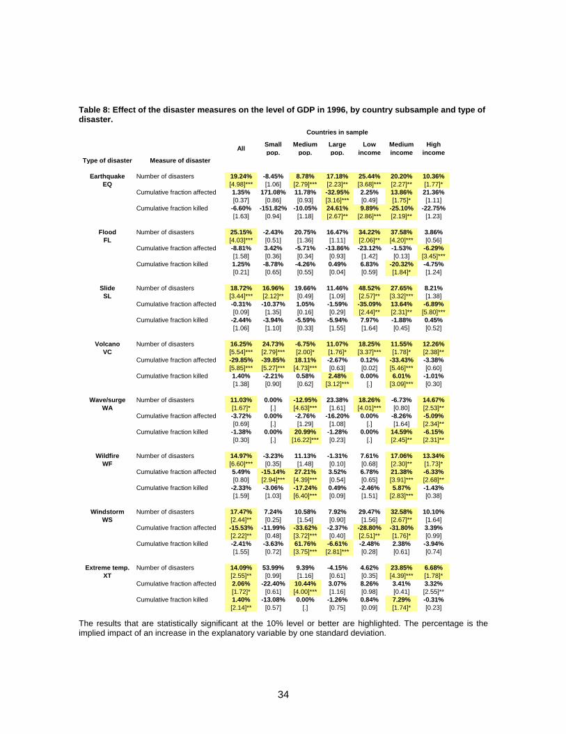
Finally, Table 8 reports similar calculations for each type of disaster and each country

subsample.

4.2 Panel Data Specification In the panel-data specification, I include country fixed effects on the right hand side to

control for land area and other unchanging, unobservable features of the countries. Year-

fixed effects account for worldwide phenomena that affect all countries in any given year.

Foreign aid as a fraction of GDP is also an explanatory variable, implicitly assuming that

14 This is a table of equivalent annualized growth rates. I f the world GDP per capita

grew annually 0.0% 0.5% 1.0% 1.5% 2.0% 2.5% 3.0%

And you added extra After 36 years, you'd get a level of GDP that was higher by0.10% 3.7% 4.4% 5.2% 6.2% 7.3% 8.7% 10.3%0.20% 7.5% 8.9% 10.6% 12.6% 14.9% 17.7% 21.0%0.30% 11.4% 13.6% 16.1% 19.2% 22.7% 27.0% 32.0%0.40% 15.5% 18.4% 21.9% 26.0% 30.9% 36.6% 43.4%0.50% 19.7% 23.4% 27.8% 33.1% 39.3% 46.6% 55.2%0.60% 24.0% 28.6% 34.0% 40.4% 48.0% 56.9% 67.4%0.70% 28.5% 34.0% 40.4% 48.0% 56.9% 67.5% 80.0%0.80% 33.2% 39.5% 47.0% 55.8% 66.3% 78.6% 93.1%0.90% 38.1% 45.3% 53.8% 63.9% 75.9% 90.0% 106.6%1.00% 43.1% 51.2% 60.9% 72.3% 85.8% 101.8% 120.6%

Between 1960 and 1996, the world's per capita GDP grew at an annualized rate of 2%.

18

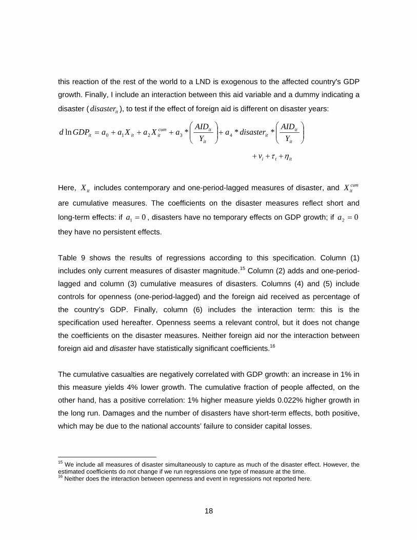
this reaction of the rest of the world to a LND is exogenous to the affected country's GDP

growth. Finally, I include an interaction between this aid variable and a dummy indicating a

disaster ( itdisaster ), to test if the effect of foreign aid is different on disaster years:

⎟⎟⎠

⎞⎜⎜⎝

⎛+⎟⎟

⎠

⎞⎜⎜⎝

⎛+++=

it

itit

it

itcumititit Y

AIDdisastera

YAID

aXaXaaGDPd ***ln 43210

ittiv ητ +++

Here, itX includes contemporary and one-period-lagged measures of disaster, and cumitX

are cumulative measures. The coefficients on the disaster measures reflect short and

long-term effects: if 01 =a , disasters have no temporary effects on GDP growth; if 02 =a

they have no persistent effects.

Table 9 shows the results of regressions according to this specification. Column (1)

includes only current measures of disaster magnitude.15 Column (2) adds and one-period-

lagged and column (3) cumulative measures of disasters. Columns (4) and (5) include

controls for openness (one-period-lagged) and the foreign aid received as percentage of

the country’s GDP. Finally, column (6) includes the interaction term: this is the

specification used hereafter. Openness seems a relevant control, but it does not change

the coefficients on the disaster measures. Neither foreign aid nor the interaction between

foreign aid and disaster have statistically significant coefficients.16

The cumulative casualties are negatively correlated with GDP growth: an increase in 1% in

this measure yields 4% lower growth. The cumulative fraction of people affected, on the

other hand, has a positive correlation: 1% higher measure yields 0.022% higher growth in

the long run. Damages and the number of disasters have short-term effects, both positive,

which may be due to the national accounts’ failure to consider capital losses.

15 We include all measures of disaster simultaneously to capture as much of the disaster effect. However, the estimated coefficients do not change if we run regressions one type of measure at the time. 16 Neither does the interaction between openness and event in regressions not reported here.

19

The regression specification in column (6) of Table 9 is carried out for each country

subsample in Table 10. The impact pattern varies depending on country population and

income level. Small and medium-population countries (columns 1 and 2) seem affected by

the fraction of people killed, although only medium-population countries show a long-term

impact (negative). For countries with large populations (column 3), on the other hand, the

fraction of people affected is relevant both in the short and long term, and the long-term

effect is positive.

The picture changes if the countries are grouped according to per capita income.

Countries in the bottom third (column 4) show no statistically significant correlation

between the disaster measures and GDP growth. Medium and high-income countries, in

columns 5 and 6, show short-term effects. High-income countries also show a persistent

effect corresponding to roughly 0.5% higher growth by 1996 for the average country in the

group.17

The final set of regressions, in Table 11, examines the effect of each type of disaster on

GDP growth using a panel specification. In each column, the sample includes all available

countries. For instance, the capital losses due to earthquakes (EQ) have a negative short-

term effect on growth. However, the impact on labor (deaths and affected) has persistent

growth effects, positive in the case of affected and negative for casualties.

Given the prior evidence and their economic meaning, the most interesting results are the

coefficients for long-term effects. Floods (FL) have no statistically significant long-term

relationship with growth. The damages due to slides (SL), on the other hand, do decrease

the growth rate. deaths due to wind storms (WS) and wild fires (WF) are correlated with

higher and extreme temperatures (XT) with lower growth. Extreme temperatures also

decrease growth through the fraction of people affected. Finally, the numbers of tsunamis

(WA) and extreme temperatures are correlated with higher persistent growth, while that of

wild fires is correlated with lower growth.

17 The average country in the high-income group has 40 disasters at the end of the period. The country with the most disasters has 272.

20

While the directions of the effects are interesting, their economic relevance depends on

their actual magnitudes and their ability to explain the observed variation in GDP growth

rates. These depend in turn on the values of the variables by the year 1996 and the

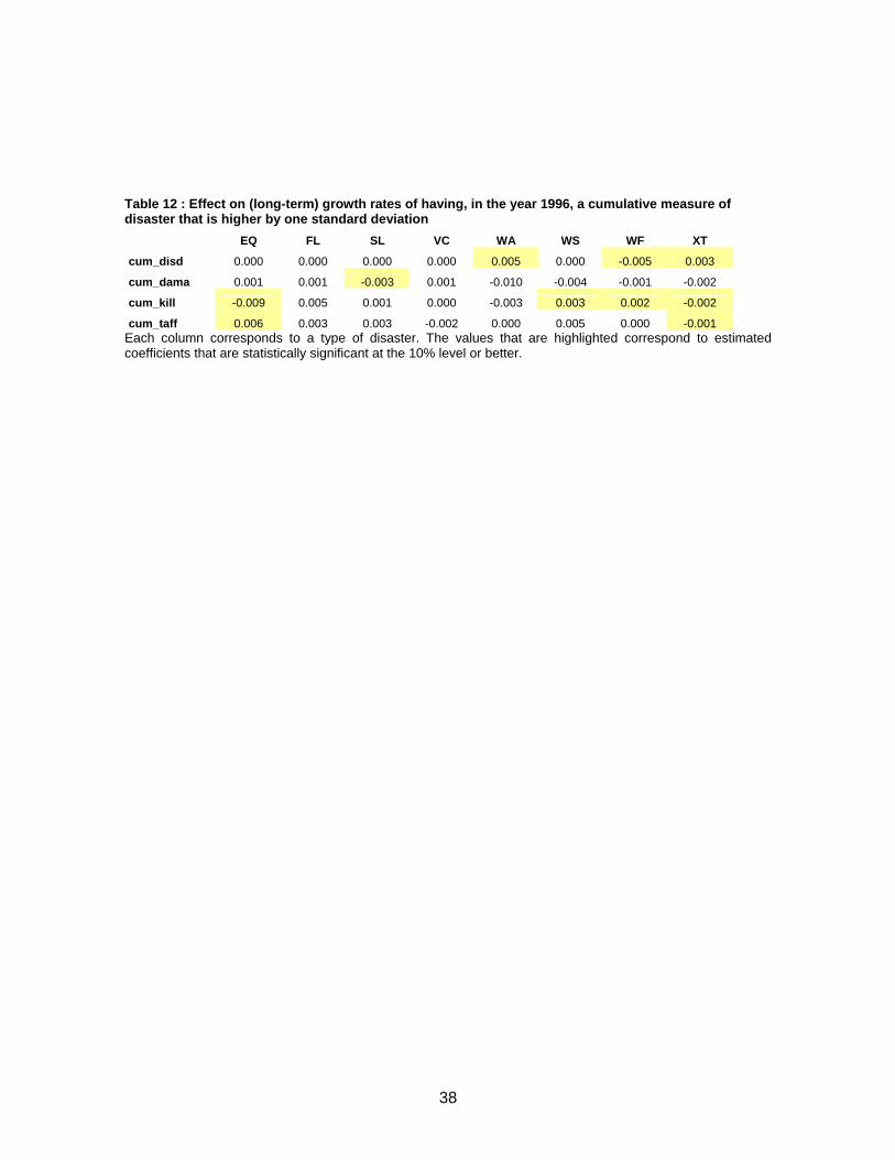
sample variation in those values. Table 12 shows the change in the long-term growth rate

of a country if the value of the cumulative disaster measures increased by one standard

deviation (of the 1996 levels). The estimated effects are not negligible: they range between

a decrease of 0.9% (casualties due to earthquakes) and an increase of 0.6% (affected

population, also due to earthquakes).

A word of caution regarding these long-term effects of LNDs. As mentioned in the

discussion of the data, a country that suffers regularly from earthquakes is likely to build its

infrastructure accordingly. This awareness of the likelihood of suffering a disaster is thus a

fixed country effect. The disaster measures do not capture it. Rather, they capture the

effect having the disaster in one year and not another; and it is well so, for it is the timing

of the earthquakes that is really exogenous in the econometric sense.

The same argument applies to some extent to all disasters. However, this interpretation of

the measures poses some difficulties for the long-term effects identified in the estimation.

How can the timing of the disasters affect the long-term growth? Is it perhaps related to the

institutional ability of the country to cope with the disasters –as suggested by the case

studies and the microeconomic literature? The answer to this question is beyond the

scope of this paper.

21

5. Concluding remarks This paper attempts to determine if there are short and long-term effects of large natural

disasters (LNDs) on GDP growth in a large panel of countries. The disasters examined are

earthquakes, floods, slides, volcano eruptions, tsunamis, wind storms, wild fires and

extreme temperatures. The paper uses original panel data on recorded disaster events

from EM-DAT: The OFDA/CRED International Disaster Database and macroeconomic

variables of 113 countries from the Penn World Tables 6.0. The data covers the period

between 1960 and 1996.

As a first approximation, I examine the relationship between the disasters that occurred in

the period 1960–1996 and the countries’ per capita GDP level in 1996. The cross-section

regression results show large and mostly positive level effects. However, these effects are

associated with the number of LNDs, rather than with the measures of their impact on the

population or capital stock.

Then, using a panel data regression with fixed country effects and year-dummies, and

controlling for trade openness and foreign aid, I test for the effect of a disaster on current

and next-year GDP growth (short-run effects) and for cumulative effects of disasters (long-

run effects). The results suggest a heterogeneous pattern of short and long-term impact of

LNDs, depending on the per capita GDP, the size of the countries studied and the type of

LND. Overall, and contrary to previous research, LNDs appear to have persistent effects

on the rate of GDP growth in the period between 1960 and 1996. These effects range from

a decrease of 0.9% to an increase of 0.6%, depending on the type of disaster.

Several features of the data advise caution in the interpretation of these results. First,

national accounts usually fail to include capital losses due to disasters, but they do include

the additional investment activity in the disaster’s aftermath. Also, this investment to

rebuild capital may span several years, depending on the type of disaster and the exact

month of the year the disaster happens.

22

A second concern is that there is an increase in the yearly number of countries reporting

disasters and in the yearly number of disasters reported in the 36-year period. This may

signal institutional development in the countries, population growth, or simply more

economic activity. Thus, the disaster measures may be endogenous to some extent.

In addition, the impact of those disasters, as measured by the peopled affected, people

killed and damages, changes substantially. Again, this may be due to development.

However, these changes seem to be related to increases in foreign aid flows. One

possible interpretation is then strategic reporting of disasters by the national governments.

A final issue is what the exogenous measures of disaster actually capture. I argue that

they capture whether a disaster happens in one year or the next: they do not capture the

fact that disasters of a certain type tend to occur in a given country, which fixed country

effects. Thus, the source of identification of disaster impact is the timing of the events. It is

not clear how this timing may affect long-term growth.

An important clarification is necessary about the interpretation of the results. Even when

the estimated effects are possitive, by no means do they mean that the overall welfare

effects of LNDs are positive. The analysis focuses on variables that are only imperfectly

correlated with welfare.

Ultimately, this paper suggests that, for the economist, natural disasters are perhaps

natural macroeconomic experiments that may help to further understand the determinants

of growth. The insights from the large literature on disasters and development should

guide macroeconomic modelling in this context. The role of institutions in the affected

country needs to be accounted for explicitly. The different build-up times and aftermaths of

the disasters may imply differences in their overall impact. The reaction of consumption

and investment patterns after a disaster may be a determinant of its long-term effect on

growth. In the area of investment, the differential effects on the types of physical capital

are of interest. Is it the case that reconstruction after a disaster concentrates in different

23

economic activities from those before? How do human capital investment and –more

controversial perhaps– social networks affect the effects of LNDs? These are possible

avenues for future research.

24

References

Albala-Bertrand, J.M. 1993. Political Economy of Large Natural Disasters. Oxford:

Clarendon Press.

Alesina, A. and D. Dollar 1998. Who Gives Foreign Aid to Whom and Why? NBER

Working Paper 6612.

Auffret, P. 2003a. High consumption Volatility: The Impact of Natural Disasters?. World

Bank Policy Research Working Paper 2962.

–––––– 2003b. Catastrophe Insurance Markets in the Caribbean Region: Market Failures

and Recommendations for Policy Interventions. World Bank Policy Research

Working Paper 2963.

Burnside, C. and D. Dollar 2000. Aid, Policies, and Growth. The American Economic

Review 90(4), pp. 847-868

Charvériat, C. 2000. Natural Disasters in Latin America and the Caribbean: An Overview

of Risk. Inter-American Development Bank Working Paper 434.

Christiano, L. and M. Eichenbaum 1989. Unit Roots in GDP: Do We Know and Do We

Care? NBER Working Paper 3130.

Easterly, W. 2003. Can Foreign Aid Buy Growth? Journal of Economic Perspectives, Vol.

17, No. 3, pp. 23-48.

Fafchamps, M. y S. Lund 2002. Risk-sharing Networks in Rural Philippines. Journal of

Development Economics 71:261-287.

Horwich, G. 2000. Economic Lessons of the Kobe Earthquake. Economic Development

and Cultural Change, Vol. 48, No. 3, pp. 521-542

Jacoby, H. y E. Skoufias 1997. Risk, Financial Markets, and Human Capital in a

Developing Country. Review of Economic Studies 64(3): 311-335.

Jalan, J. y M. Ravallion 2001. Behavioral Responses to Risk in China. Journal of

Development Economics 66: 23-49.

Jensen, R. 2000. Agricultural Volatility and Investments in Children The American

Economic Review, 90(2): 399-404.

25

Raddatz, C. 2005. Are External Shocks Responsible for the Instability of Output in Low-

income Countries? World Bank, Development Economics Research Group

WPS3680.

Rosenzweig, M. y O. Stark 1989. Consumption Smoothing, Migration and Marriage:

Evidence from Rural India. The Journal of Political Economy 97(4):905-926.

Weder, B. 2000. Foreign Aid, Institutions and Development. Paper presented at the UNU

Millennium Conference in Tokyo, Japan.

26

Figures and Tables

Table 1 : Disaster types

NATURAL TECHNOLOGICAL CONFLICT Drought Industrial accident Civil disturbance Earthquake (460) Miscellaneous accident Civil strife Epidemic Transport accident Displaced Extreme temperature (141) International conflict Famine Insect infestation Flood (1285) Slide (241) Volcano (115) Wave/surge (20) Wild fire (160) Wind storm (1271)

These are the types of disaster for which events are recorded in EM-DAT. Those shaded are the ones used, and the figure in parenthesis is the number of events reported in the period 1960-1998 for the countries in our sample.

Figure 1: Frequency of events by type and region

D is a s t e r f r e q u e n c i e s b y r e g i o n

0

1 0 0

2 0 0

3 0 0

4 0 0

5 0 0

6 0 0

7 0 0

8 0 0

9 0 0

Afric

a

Cen

tral A

frica

East

Afri

ca

Nor

th A

frica

Sout

hern

Afri

ca

Wes

t Afri

ca

Amer

icas

Cen

tral A

mer

ica

Nor

th A

mer

ica

Sout

h Am

eric

a

Car

ibbe

an

Asia

East

Asi

a

Sout

h As

ia

Sout

h-ea

st A

sia

Wes

t Asi

a

Euro

pe

Euro

pean

Uni

on

Res

t of E

urop

e

Rus

sian

Fed

erat

ion

Oce

ania

R e g i o n

Num

ber o

f eve

nts

W in d s t o r mW i ld f i r eW a v e / s u r g eV o l c a n oS l i d eF lo o dE x t r e m e t e m pE a r t h q u a k e

These are the events used in the regressions.

27

Table 2: Correlation among aggregate disaster measures dama kill taff disd

dama 1 kill 0.2215* 1 taff 0.3388* 0.3478* 1 disd 0.0622* 0.0558* 0.1652* 1

(*) significant at the 5% level.

Figure 2: Reported events by year

R e p o r t s o f d i s a s t e r s

0

2 0

4 0

6 0

8 0

1 0 0

1 2 0

1 4 0

1 6 0

1 8 0

1 9 6 01 9 6 1

1 9 6 21 9 6 3

1 9 6 41 9 6 5

1 9 6 61 9 6 7

1 9 6 81 9 6 9

1 9 7 01 9 7 1

1 9 7 21 9 7 3

1 9 7 41 9 7 5

1 9 7 61 9 7 7

1 9 7 81 9 7 9

1 9 8 01 9 8 1

1 9 8 21 9 8 3

1 9 8 41 9 8 5

1 9 8 61 9 8 7

1 9 8 81 9 8 9

1 9 9 01 9 9 1

1 9 9 21 9 9 3

1 9 9 41 9 9 5

1 9 9 61 9 9 7

1 9 9 8

Y e a r

Freq

uenc

y

R e p o r t in g c o u n t r ie s E v e n t s r e p o r t e d

These are only the types of events used in the regressions, and only for the countries included in the sample.

28

Figure 3: GDP per capita vs. number of reported disaster events

Figure 4 : Number of reported disasters by type

D is a s t e r r e p o r t s

0

1 0

2 0

3 0

4 0

5 0

6 0

7 0

8 0

1960

1962

1964

1966

1968

1970

1972

1974

1976

1978

1980

1982

1984

1986

1988

1990

1992

1994

1996

1998

Y e a r

E QF LS LV CW AW FW SX T

29

Figure 5: Reported impact of disasters

Upper panel: Fraction of the population affected and killed. Lower panel: Damages as a fraction of GDP.

Im p a c t r e p o r t s

0

1 0

2 0

3 0

4 0

5 0

6 0

1 9 6 01 9 6 2

1 9 6 41 9 6 6

1 9 6 81 9 7 0

1 9 7 21 9 7 4

1 9 7 61 9 7 8

1 9 8 01 9 8 2

1 9 8 41 9 8 6

1 9 8 81 9 9 0

1 9 9 21 9 9 4

1 9 9 61 9 9 8

Y e a r

Kill

ed/A

ffec

ted

K i l le d p e r m i l l io nA f f e c t e d p e r 1 ' 0 0 0

Im p a c t r e p o r t s

0

0 . 2

0 . 4

0 . 6

0 . 8

1

1 . 2

1 . 4

1 . 6

1 . 8

1 9 6 01 9 6 2

1 9 6 41 9 6 6

1 9 6 81 9 7 0

1 9 7 21 9 7 4

1 9 7 61 9 7 8

1 9 8 01 9 8 2

1 9 8 41 9 8 6

1 9 8 81 9 9 0

1 9 9 21 9 9 4

1 9 9 61 9 9 8

Y e a r

Dam

ages

per

trill

ion

D a m a g e s p e r t r i l l i o n

30

Table 3: Probability of a country reporting at least a disaster.

DEPVAR: 1 if country reported a disaster

(1) (2) (3) (4) (5) (6) (7)

lnPOP 2.530 2.405 1.537 1.569 -0.602 -0.838 (12.16)** (9.65)** (5.41)** (5.24)** (1.30) (1.75) lnYpc 0.304 0.314 -0.041 -0.064 -0.684 -0.873 (1.85) (1.77) (0.23) (0.33) (3.15)** (3.89)** lag of own AID 3.154 -1.302 -2.953 -2.594 (0.83) (0.32) (0.73) (0.65) lag of world AID 631.788 639.547 286.681 33.650 (5.20)** (5.13)** (2.08)* (0.21) trend 0.063 0.077 0.163 (16.15)** (6.09)** (5.53)** trend^2 -0.002 (3.27)** Observations 4134 4027 3921 3929 3921 3921 3921 Number of isogrp 106 106 106 106 106 106 106 R-squared Absolute value of z statistics in parentheses * significant at 5%; ** significant at 1%

Panel data logit model with country FE. I report the odds ratios (change in p/1-p). The data includes years

1960-1996.

31

Table 4: Number of reported events by year DEPVAR: number of disasters reported by a country

(1) (2) (3) (4)

lnPOP 0.283 0.303 0.312 0.312 (2.96)** (3.11)** (3.26)** (3.24)** lnYpc -0.436 -0.433 -0.444 -0.429 (5.05)** (4.63)** (5.01)** (4.59)** lag of own AID 1.550 1.178 (0.60) (0.45) lag of world AID 88.012 85.128 (1.30) (1.25) trend 0.103 0.105 0.095 0.094 (11.08)** (10.52)** (7.10)** (7.03)** trend^2 -0.001 -0.001 -0.001 -0.001 (7.58)** (7.44)** (5.45)** (5.42)** Observations 4105 3997 4005 3997 Number of isogrp 108 108 108 108 R-squared Absolute value of z statistics in parentheses * significant at 5%; ** significant at 1% Model Neg Bin Neg Bin Neg Bin Neg Bin Country fixed effects Yes Yes Yes Yes

The model estimates the expected number of events reported by a negative binomial regression. The coefficients are incidence rate ratios, interpreted as the change in the expected number of events due to a unit increase in the regressor.

32

Table 5: Cross-country regression of GDP level in 1996. (1) (2) (3) (4) lnGDP1996 lnGDP1996 lnGDP1996 lnGDP1996 lnGDP1960 0.992 1.006 1.009 0.967 [12.45]*** [11.22]*** [11.47]*** [12.39]*** lnPOPgrowth -0.269 -0.324 -0.318 -0.256 [2.35]** [2.61]** [2.57]** [2.33]** lnAREA -0.103 -0.070 -0.069 -0.118 [3.14]*** [1.97]* [1.97]* [3.55]*** Number of disasters 0.004 0.006 [3.79]*** [4.32]*** Cumul. fraction affected -0.026 -0.296 [0.41] [2.15]** Cumul. fraction killed -21.809 3.986 [0.78] [0.09] Constant 2.075 1.773 1.744 2.464 [2.83]*** [2.21]** [2.24]** [3.28]*** Observations 102 102 102 102 R-squared 0.76 0.73 0.73 0.77 Robust t statistics in brackets * significant at 10%; ** significant at 5%; *** significant at 1% The sample includes all countries.

33

Table 6: Effect of the disaster measures on the level of GDP in 1996. Implied impact on 1996 GDP level

(1) (2) (3) (4) Number of disasters 19.81% 29.72% [3.79]*** [4.32]*** Cumul. fraction affected -1.22% -13.93% [0.41] [2.15]** Cumul. fraction killed -2.47% 0.45% [0.78] [0.09]

Robust t statistics in brackets * significant at 10%; ** significant at 5%; *** significant at 1%

The results that are statistically significant at the 10% level or better are highlighted. The percentage is the implied impact of an increase in the explanatory variable by one standard deviation.

Table 7: Effect of the disaster measures on the level of GDP in 1996, by country subsample.

Implied impact on GDP level (1) (2) (3) (4) (5) (6)

Number of disasters 0.00% 18.90% 13.55% 39.93% 38.55% 11.14% [0.03] [2.15]** [1.48] [2.51]** [3.54]*** [1.90]* Cumul. fraction affected -5.05% -15.31% -16.00% -60.01% -25.93% -0.26% [0.60] [0.94] [1.64] [1.45] [1.80]* [0.05] Cumul. fraction killed -12.43% 11.67% 2.57% 37.73% -3.21% -3.37% [1.85]* [1.07] [0.37] [1.07] [0.40] [0.65] Robust t statistics in brackets

Countries in sample Small pop Medium pop Large pop Low

income Medium income

High income

The results that are statistically significant at least at the 10% level are highlighted. The percentage is the implied impact of an increase in the explanatory variable by one standard deviation.

34

Table 8: Effect of the disaster measures on the level of GDP in 1996, by country subsample and type of disaster.

All Small pop.

Medium pop.

Large pop.

Low income

Medium income

High income

Type of disaster Measure of disaster

Earthquake Number of disasters 19.24% -8.45% 8.78% 17.18% 25.44% 20.20% 10.36%EQ [4.98]*** [1.06] [2.79]*** [2.23]** [3.68]*** [2.27]** [1.77]*

Cumulative fraction affected 1.35% 171.08% 11.78% -32.95% 2.25% 13.86% 21.36%[0.37] [0.86] [0.93] [3.16]*** [0.49] [1.75]* [1.11]

Cumulative fraction killed -6.60% -151.82% -10.05% 24.61% 9.89% -25.10% -22.75%[1.63] [0.94] [1.18] [2.67]** [2.86]*** [2.19]** [1.23]

Flood Number of disasters 25.15% -2.43% 20.75% 16.47% 34.22% 37.58% 3.86%FL [4.03]*** [0.51] [1.36] [1.11] [2.06]** [4.20]*** [0.56]

Cumulative fraction affected -8.81% 3.42% -5.71% -13.86% -23.12% -1.53% -6.29%[1.58] [0.36] [0.34] [0.93] [1.42] [0.13] [3.45]***

Cumulative fraction killed 1.25% -8.78% -4.26% 0.49% 6.83% -20.32% -4.75%[0.21] [0.65] [0.55] [0.04] [0.59] [1.84]* [1.24]

Slide Number of disasters 18.72% 16.96% 19.66% 11.46% 48.52% 27.65% 8.21%SL [3.44]*** [2.12]** [0.49] [1.09] [2.57]** [3.32]*** [1.38]

Cumulative fraction affected -0.31% -10.37% 1.05% -1.59% -35.09% 13.64% -6.89%[0.09] [1.35] [0.16] [0.29] [2.44]** [2.31]** [5.80]***

Cumulative fraction killed -2.44% -3.94% -5.59% -5.94% 7.97% -1.88% 0.45%[1.06] [1.10] [0.33] [1.55] [1.64] [0.45] [0.52]

Volcano Number of disasters 16.25% 24.73% -6.75% 11.07% 18.25% 11.55% 12.26%VC [5.54]*** [2.79]*** [2.00]* [1.76]* [3.37]*** [1.78]* [2.38]**

Cumulative fraction affected -29.85% -39.85% 18.11% -2.67% 0.12% -33.43% -3.38%[5.85]*** [5.27]*** [4.73]*** [0.63] [0.02] [5.46]*** [0.60]

Cumulative fraction killed 1.40% -2.21% 0.58% 2.48% 0.00% 6.01% -1.01%[1.38] [0.90] [0.62] [3.12]*** [.] [3.09]*** [0.30]

Wave/surge Number of disasters 11.03% 0.00% -12.95% 23.38% 18.26% -6.73% 14.67%WA [1.67]* [.] [4.63]*** [1.61] [4.01]*** [0.80] [2.53]**

Cumulative fraction affected -3.72% 0.00% -2.76% -16.20% 0.00% -8.26% -5.09%[0.69] [.] [1.29] [1.08] [.] [1.64] [2.34]**

Cumulative fraction killed -1.38% 0.00% 20.99% -1.28% 0.00% 14.59% -6.15%[0.30] [.] [16.22]*** [0.23] [.] [2.45]** [2.31]**

Wildfire Number of disasters 14.97% -3.23% 11.13% -1.31% 7.61% 17.06% 13.34%WF [6.60]*** [0.35] [1.48] [0.10] [0.68] [2.30]** [1.73]*

Cumulative fraction affected 5.49% -15.14% 27.21% 3.52% 6.78% 21.38% -6.33%[0.80] [2.94]*** [4.39]*** [0.54] [0.65] [3.91]*** [2.68]**

Cumulative fraction killed -2.33% -3.06% -17.24% 0.49% -2.46% 5.87% -1.43%[1.59] [1.03] [6.40]*** [0.09] [1.51] [2.83]*** [0.38]

Windstorm Number of disasters 17.47% 7.24% 10.58% 7.92% 29.47% 32.58% 10.10%WS [2.44]** [0.25] [1.54] [0.90] [1.56] [2.67]** [1.64]

Cumulative fraction affected -15.53% -11.99% -33.62% -2.37% -28.80% -31.80% 3.39%[2.22]** [0.48] [3.72]*** [0.40] [2.51]** [1.76]* [0.99]

Cumulative fraction killed -2.41% -3.63% 61.76% -6.61% -2.48% 2.38% -3.94%[1.55] [0.72] [3.75]*** [2.81]*** [0.28] [0.61] [0.74]

Extreme temp. Number of disasters 14.09% 53.99% 9.39% -4.15% 4.62% 23.85% 6.68%XT [2.55]** [0.99] [1.16] [0.61] [0.35] [4.39]*** [1.78]*

Cumulative fraction affected 2.06% -22.40% 10.44% 3.07% 8.26% 3.41% 3.32%[1.72]* [0.61] [4.00]*** [1.16] [0.98] [0.41] [2.55]**

Cumulative fraction killed 1.40% -13.08% 0.00% -1.26% 0.84% 7.29% -0.31%[2.14]** [0.57] [.] [0.75] [0.09] [1.74]* [0.23]

Countries in sample

The results that are statistically significant at the 10% level or better are highlighted. The percentage is the implied impact of an increase in the explanatory variable by one standard deviation.

35

Table 9: Panel regression of GDP growth on disasters. Dep var: Growth in per capita GDP

(1) (2) (3) (4) (5) (6)

cum_disd -0.000 -0.000 -0.000 -0.000[0.000] [0.000] [0.000] [0.000]

cum_dama -33.583 -27.624 -26.995 -24.845[43.646] [44.090] [44.017] [44.657]

cum_kill -4.932 -4.082 -4.100 -4.000[2.161]** [2.194]* [2.197]* [2.207]*

cum_taff 0.023 0.022 0.022 0.022[0.007]*** [0.007]*** [0.007]*** [0.007]***

disd 0.002 0.001 0.001 0.001 0.001 0.001[0.001]*** [0.001] [0.001] [0.001] [0.001] [0.001]*

dama 89.775 100.192 134.498 133.769 133.903 136.501[108.768] [108.503] [116.273] [120.571] [120.664] [119.477]

kill -1.090 -0.840 2.078 1.435 1.461 1.203[4.092] [4.331] [4.863] [4.811] [4.798] [4.862]

taff 0.009 0.010 -0.008 -0.011 -0.011 -0.009[0.027] [0.027] [0.029] [0.030] [0.030] [0.030]

disd [t-1] 0.002 0.002 0.002 0.002 0.002[0.001]*** [0.001]*** [0.001]*** [0.001]*** [0.001]***

dama [t-1] 91.741 123.042 127.843 127.952 126.276[61.393] [71.709]* [73.222]* [73.182]* [73.809]*

kill [t-1] 1.900 4.897 4.210 4.242 4.140[5.834] [5.558] [5.585] [5.592] [5.577]

taff [t-1] -0.001 -0.019 -0.022 -0.022 -0.021[0.024] [0.025] [0.025] [0.025] [0.025]

open [t-1] 0.000 0.000 0.000[0.000]*** [0.000]*** [0.000]***

aid 0.035 0.049[0.091] [0.092]

aid*disaster -0.088[0.167]

Observations 4168 4168 4168 4168 4168 4168Number of isogrp 113 113 113 113 113 113R-squared 0.05 0.05 0.05 0.06 0.06 0.06Robust standard errors in brackets* significant at 10%; ** significant at 5%; *** significant at 1% All regressions have country and year fixed effects. [t-1] indicates the one-period lag of the variable.

36

Table 10: Panel regression of GDP growth on disasters, by groups of countries. Dep var: Growth in per capita GDP

(1) (2) (3) (4) (5) (6)

Countries in sample Small pop Medium pop Large pop Low income Medium

income High income

cum_disd 0.00041 -0.00026 -0.00003 0.00002 -0.00010 -0.00012[0.00032] [0.00019] [0.00007] [0.00012] [0.00011] [0.00006]**

cum_dama 0.462 54.482 -110.146 130.159 -75.675 209.962[139.213] [142.716] [208.580] [120.318] [98.844] [167.004]

cum_kill -2.489 -12.237 -5.144 -2.818 -1.259 -1.394[5.447] [6.321]* [3.407] [4.987] [2.750] [38.330]

cum_taff 0.014 0.046 0.028 0.012 0.013 0.013[0.020] [0.035] [0.008]*** [0.013] [0.014] [0.022]

disd 0.001 -0.000 0.001 0.003 0.002 0.001[0.003] [0.002] [0.001] [0.002] [0.001] [0.001]

dama 16.102 -440.710 -672.279 -486.086 151.013 -561.659[212.179] [301.510] [465.889] [528.947] [231.836] [263.266]**

kill -17.262 23.644 5.318 5.844 -0.146 -79.817[6.454]*** [14.294]* [4.115] [6.720] [6.032] [77.120]

taff 0.054 -0.044 0.062 0.059 -0.037 0.100[0.035] [0.067] [0.048] [0.049] [0.036] [0.031]***

disd [t-1] 0.002 0.004 0.001 0.003 0.002 0.001[0.003] [0.002]** [0.001] [0.002] [0.001]* [0.001]*

dama [t-1] -79.633 -424.976 362.993 -53.090 476.749 -142.237[295.184] [411.124] [631.440] [808.257] [255.625]* [229.612]

kill [t-1] 4.870 25.313 0.153 3.562 1.882 6.467[8.288] [25.100] [6.987] [15.466] [5.268] [27.598]

taff [t-1] 0.030 -0.031 -0.049 -0.040 -0.055 0.040[0.041] [0.135] [0.028]* [0.035] [0.050] [0.050]

open [t-1] 0.000 0.000 0.000 0.000 0.000 0.001[0.000]*** [0.000] [0.000] [0.000] [0.000]* [0.000]***

aid 0.196 0.054 -1.005 -0.095 0.234 -0.523[0.128] [0.175] [0.467]** [0.155] [0.146] [0.410]

aid*disaster -0.514 0.485 0.322 -0.154 -0.204 1.106[0.247]** [0.218]** [0.603] [0.261] [0.207] [0.502]**

Observations 1321 1321 1329 1329 1322 1289Number of isogrp 35 35 35 35 35 34R-squared 0.09 0.08 0.11 0.06 0.08 0.17Robust standard errors in brackets* significant at 10%; ** significant at 5%; *** significant at 1% All regressions have country and year fixed effects. [t-1] indicates the one-period lag of the variable.

37

Table 11: Panel regression of GDP growth on disasters, by type of disaster. Dep var: Growth in per capita GDP

(1) (2) (3) (4) (5) (6) (7) (8)EQ FL SL VC WA WS WF XT

cum_disd -0.000 0.000 0.000 -0.000 0.008 -0.000 -0.001 0.001[0.000] [0.000] [0.001] [0.001] [0.004]* [0.000] [0.000]* [0.001]***

cum_dama 97.699 152.222 -2,315.337 97.119 -877,287.511 -74.044 -518.302 -714.685[165.020] [232.298] [958.243]** [192.295] [733,248.454] [62.754] [1,199.007] [658.527]

cum_kill -11.876 67.492 7.327 2.635 -181.984 4.417 1,991.177 -174.182[4.267]*** [46.485] [8.449] [13.739] [113.565] [2.086]** [1,165.592]* [79.193]**

cum_taff 0.058 0.009 0.657 -0.066 1.266 0.018 0.126 -0.046[0.025]** [0.008] [0.436] [0.163] [18.674] [0.014] [1.888] [0.026]*

disd 0.005 0.001 0.003 0.001 0.000 0.002 -0.001 -0.004[0.002]*** [0.002] [0.003] [0.004] [0.010] [0.001] [0.003] [0.004]

dama -697.719 -1,364.951 1,424.942 284.050 377,733.873 266.009 1,177.754 5,034.503[248.025]*** [547.936]** [1,871.188] [310.068] [904,575.871] [109.830]** [1,467.356] [600.221]***

kill 0.509 152.992 11.461 25.431 194.925 -3.451 -4,598.006 -199.716[4.721] [109.993] [14.414] [59.525] [147.341] [7.297] [9,126.668] [81.367]**

taff 0.079 0.028 -0.527 0.097 -21.550 -0.036 2.774 0.277[0.043]* [0.031] [0.515] [0.096] [30.843] [0.037] [2.085] [0.049]***

disd [t-1] 0.002 0.003 0.005 0.003 -0.009 0.002 0.003 0.002[0.002] [0.001]** [0.003]* [0.005] [0.011] [0.001]* [0.003] [0.003]

dama [t-1] 259.877 729.963 2,585.924 -376.040 565,978.829 157.245 -3,023.566 1,124.962[283.961] [585.457] [1,381.494]* [370.269] 132,276.453]** [94.446]* [3,168.671] [572.793]**

kill [t-1] 12.532 33.695 -38.009 3.455 198.702 -12.581 4,878.326 186.601[8.447] [67.184] [18.174]** [19.240] [114.108]* [6.610]* [1,868.334]*** [85.669]**

taff [t-1] -0.049 -0.087 -0.235 -0.083 -19.888 -0.002 -1.228 0.211[0.052] [0.036]** [0.409] [0.131] [26.504] [0.036] [2.155] [0.067]***

open [t-1] 0.000 0.000 0.000 0.000 0.000 0.000 0.000 0.000[0.000]*** [0.000]*** [0.000]*** [0.000]*** [0.000]*** [0.000]*** [0.000]*** [0.000]***

aid 0.028 0.048 0.035 0.026 0.025 0.037 0.019 0.038[0.092] [0.092] [0.092] [0.091] [0.091] [0.091] [0.091] [0.091]

aid*disaster -0.040 -0.094 -0.047 -0.040 -0.040 -0.065 -0.038 -0.050[0.162] [0.165] [0.161] [0.163] [0.160] [0.164] [0.159] [0.161]

Observations 4168 4168 4168 4168 4168 4168 4168 4168Number of isogrp 113 113 113 113 113 113 113 113R-squared 0.06 0.06 0.06 0.05 0.05 0.06 0.06 0.06Robust standard errors in brackets* significant at 10%; ** significant at 5%; *** significant at 1% All regressions have country and year fixed effects. [t-1] indicates the one-period lag of the variable. EQ: earthquake; FL. flood; SL: slide; VC: volcano; WA: wave/surge; WS: wind storm; WF: wildfire; XT: extreme temperature.

38

Table 12 : Effect on (long-term) growth rates of having, in the year 1996, a cumulative measure of disaster that is higher by one standard deviation EQ FL SL VC WA WS WF XT

cum_disd 0.000 0.000 0.000 0.000 0.005 0.000 -0.005 0.003

cum_dama 0.001 0.001 -0.003 0.001 -0.010 -0.004 -0.001 -0.002

cum_kill -0.009 0.005 0.001 0.000 -0.003 0.003 0.002 -0.002

cum_taff 0.006 0.003 0.003 -0.002 0.000 0.005 0.000 -0.001 Each column corresponds to a type of disaster. The values that are highlighted correspond to estimated coefficients that are statistically significant at the 10% level or better.

39

Appendix A: Disaster Data

The format of a disaster event entry in EM-DAT is exemplified by Table 1. The data

it may contain depends on availability:18

Typical entry in EM-DAT

18 This variable description is quoted directly from the webpage of the EM-DAT Guidelines at http://www.cred.be/emdat/intro.htm

40

The following is a short explanation for each of these variables, quoted from the EM-DAT

Guidelines:

• Country: Country in which the disaster has occurred (see Country list). If a disaster

has affected more than one country, there is one entry for each country. If the

quantitative data (killed, injured, homeless, affected, estimation of damage) are not

given by country, they will be entered under the NA-related region/continent and an

entry will be made for each country without data.

• ISO Code: Automatically linked to the country (see ISO Code list). The International

Organization for Standardization has attributed a 3-letter code to each country. CRED

is using the ISO 3166.

• Region: Automatically linked to the country (see Region list).

• Continent: Africa, Americas, Asia, Europe and Oceania are the five continents. This

field is automatically linked to the country.

• Disaster group: Three groups of disasters are distinguished in EM-DAT: natural

disasters, technological disasters and conflict. This field is automatically linked to the

disaster type.

• Disaster type: Description of the disaster according to a pre-define classification

scheme scheme (See Disaster type list). Two or more disasters may be related, i.e. a

disaster may occur as a consequence of a primary event. For example, a cyclone

may generate a flood or a landslide; or an earthquake may cause a gas line to

rupture, causing an ecological disaster. The primary disaster type is recorded first,

followed in the comments field by a related disaster description.

• Disaster subset: Specific information related to the disaster type (see Dissubset list).

• Date: When the disaster occurred. The date is entered as follow: Year/Month/Day.

This date is easily defined for all sudden disasters, but for disaster situations

developing gradually over a longer time period, only month and/or year are recorded.

The data available for long-term disaster are divided by the number of affected years

(in the chronological table of the profiles, and in the raw data). The totals of people

reported killed or affected or estimated damage are only used in the TOP 10 tables in

the disaster profiles.

41

• Killed: Persons confirmed as dead and persons missing and presumed dead (official

figures when available).

• Injured: The number of injured is entered when the term "injured" is written in the

source. Injured people are always part of the affected population. Any related word

like "hospitalized" is considered as injured. If there is no precise number like

"hundreds of injured", 200 injured will be entered (although it is probably

underestimated). Any other specification will be written in the comments field.

• Homeless: They are always part of the affected population. Reporting from the field

should give the number of individuals that are homeless; if only the number of families

or houses is reported, the figure is multiplied by the average family size for the

affected area (x5 for the developing countries, x3 for the industrialised countries,

according to UNDP country list). Any other specification will be written in the

comments field. Specific examples: Number of houses destroyed = 50 x 5 = 250

homeless (although it is probably underestimated) If the value ranging from a

minimum to a maximum: take the average Thousands of homeless = 2000 homeless

(although it is probably underestimated) Affected: People requiring immediate

assistance during a period of emergency; it can also be displaced or evacuated

people. Any other specification will be written in the comments field.

• Total affected: Sum of injured, homeless, and affected.

• Estimated Damage: Although several institutions have developed methodologies to

quantify these losses in their specific domain, no standard procedure to determine a

global figure for the economic impact exists up to now. Estimated damage are (if

available) given in 3 different currencies (in thousand):

• Dam US Dam Euros DamLocal: the local currency field is automatically linked to the

country. If cost damage is given in the local currency, it will be directly converted in

US and in EURO for European countries. For each disaster, the registered figure

corresponds to the damage value at the moment of the event, i.e. the figures are

shown true to the year of the event

• Primary source: Primary source of disaster information. A priority list as been

established (see Source list). In some specific case, a secondary source can become

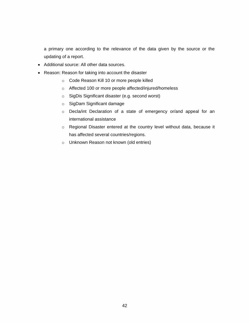
42

a primary one according to the relevance of the data given by the source or the

updating of a report.

• Additional source: All other data sources.

• Reason: Reason for taking into account the disaster

o Code Reason Kill 10 or more people killed

o Affected 100 or more people affected/injured/homeless

o SigDis Significant disaster (e.g. second worst)

o SigDam Significant damage

o Decla/int Declaration of a state of emergency or/and appeal for an

international assistance

o Regional Disaster entered at the country level without data, because it

has affected several countries/regions.

o Unknown Reason not known (old entries)

43

Appendix B: Foreign Aid Data

I use three data series from the DAC/GEO database of Geographic Distribution of

Financial Flows to Aid Recipients, 1960-1998, included in the OECD publication

International Development Statistics (IDS), edition 2000. I reproduce here the database

descriptions of this series.

Total Official Net Flows The sum of Official Development Assistance (ODA) and Other

Official Flows (OOF) represents the total net disbursements by the official sector at large

to the recipient country.

Official Development Assistance (ODA) Includes grants or loans to countries and

territories on Part I of the DAC List of Aid Recipients (developing countries) which are a)

undertaken by the official sector; b) with promotion of economic development and welfare

as the main objective, and c) at concessional financial terms (if a loan, have a grant

element of at least 25 per cent).

In addition to financial flows, Technical Co-operation is included in official aid. Grants,

loans and credits for military purposes are excluded.

Other Official Flows (OOF) Transactions by the official sector whose main objective is

other than development motivated, or, if development motivated, whose grant element is

below the 25% threshold which would make them eligible to be recorded as ODA. The

main classes of transactions included here are official export credits, official sector equity

and portfolio investment, and debt reorganisation undertaken by the official sector at non-

concessional terms (irrespective of the nature or the identity of the original creditor).

44

Appendix C: Countries in the sample

According to their population in 1960, the countries in the sample are:

Small Medium Large Not included

barbados 4 angola 1 algeria 30 antigua and 5benin 9 austria 20 argentina 47 dominica 8botswana 3 bolivia 22 australia 169 grenada 4cape verde 4 burkina faso 4 bangladesh 136 saint kitts 5central afri 4 burundi 1 belgium 20 saint vincen 9comoros 6 cameroon 5 brazil 84 sao tome and 0congo 1 chad 6 canada 53 sierra leone 3costa rica 31 chile 44 colombia 80 tunisia 11cyprus 4 cote d'ivoir 2 egypt 15equatorial g 0 denmark 9 france 66fiji 30 dominican re 20 greece 44gabon 1 ecuador 52 india 236gambia 2 el salvador 12 indonesia 153guinea-bissa 2 finland 1 italy 65guyana 3 ghana 5 japan 132honduras 25 guatemala 20 kenya 7iceland 10 guinea 3 korea, repub 44israel 7 haiti 28 mexico 92jamaica 17 hong kong 184 morocco 18jordan 9 ireland 6 nepal 41lesotho 6 madagascar 21 netherlands 11luxembourg 3 malawi 8 nigeria 6mauritania 3 malaysia 16 pakistan 58mauritius 18 mali 2 peru 68namibia 0 mozambique 15 philippines 215new zealand 66 niger 3 south africa 29nicaragua 20 norway 5 spain 40panama 13 senegal 7 sri lanka 32papua new gu 33 sweden 7 taiwan, prov 31paraguay 11 switzerland 25 tanzania, un 16seychelles 0 syrian arab 3 thailand 36singapore 0 uganda 5 turkey 50togo 3 venezuela 13 united kingd 31trinidad and 9 zambia 2 united state 272uruguay 4 zimbabwe 2 zaire 0

TOTAL 361 579 2427 45 Countries in the sample by 1960 population The countries are classified according to their 1960 population. Those under “Not Included” are in the sample but there was no population data for that year. The number in front of the country is the number of disasters it had in the period of analysis.

45

According to their per capita GDP in 1960, the countries in the sample are:

Poor Medium Rich Not included

bangladesh 136 algeria 30 argentina 47 antigua and 5benin 9 angola 1 australia 169 dominica 8botswana 3 bolivia 22 austria 20 grenada 4burkina faso 4 brazil 84 barbados 4 haiti 28burundi 1 cameroon 5 belgium 20 saint kitts 5cape verde 4 central afri 4 canada 53 saint vincen 9chad 6 colombia 80 chile 44 sao tome and 0congo 1 comoros 6 costa rica 31 sierra leone 3dominican re 20 cote d'ivoir 2 denmark 9 tunisia 11egypt 15 cyprus 4 el salvador 12gambia 2 ecuador 52 finland 1ghana 5 equatorial g 0 france 66guinea-bissa 2 fiji 30 greece 44india 236 gabon 1 iceland 10indonesia 153 guatemala 20 ireland 6kenya 7 guinea 3 israel 7korea, repub 44 guyana 3 italy 65lesotho 6 honduras 25 japan 132madagascar 21 hong kong 184 luxembourg 3malawi 8 jamaica 17 mauritius 18mali 2 jordan 9 mexico 92mauritania 3 malaysia 16 namibia 0morocco 18 mozambique 15 netherlands 11nepal 41 nicaragua 20 new zealand 66niger 3 panama 13 norway 5nigeria 6 papua new gu 33 south africa 29pakistan 58 paraguay 11 spain 40sri lanka 32 peru 68 sweden 7syrian arab 3 philippines 215 switzerland 25taiwan, prov 31 senegal 7 trinidad and 9tanzania, un 16 seychelles 0 united kingd 31thailand 36 singapore 0 united state 272togo 3 turkey 50 uruguay 4uganda 5 zambia 2 venezuela 13zaire 0 zimbabwe 2

TOTAL 940 1034 1365 73 Countries in the sample by per capita GDP level The countries are classified according to their 1960 per capita GDP. Those under “Not Included” are in the sample but there was no GDP data for that year. The number in front of the country is the number of disasters it had in the period of analysis.