CE 231 ENGINEERING ECONOMY BREAK-EVEN...

1

CE 231 – ENGINEERING ECONOMY

BREAK-EVEN ANALYSIS

This chapter covers the basics of break-even analysis, the simplest analytical tool in

management. It details what break-even analysis is, what it is used for, what definitions are

used in break-even analysis and how break-even analysis can be helpful in decision- making

of professionals in construction industry.

In construction industry, break-even analysis can be a handy tool to find answers to questions

such as: How many years should I operate the facility to recover the initial investment and

annual operating costs? How much does our company need to sell to reach the desired

profitability? What should be the toll rate to cover my costs?

Break-even analysis for a single project

Definitions: Basically, break-even analysis determines the “break-even point”, at which

operations neither make money nor loose money (Paek 2000, Blank and Tarquin 2008). At the

break-even point, there is no gain or loss; hence costs or expenses are equal to

revenues/incomes.

Break-even analysis utilizes two types of inputs for calculation of costs as: fixed costs and

variable costs:

Fixed cost represents the expenses that are not related with the volume of production

(or activity level) over a feasible range of operations. Examples include buildings,

insurance expenses, depreciation, overheads, cost of information systems (Blank and

Tarquin 2008). It is the sum of all costs to produce the first unit of a product. Another

example could be the cost of an excavation equipment regardless of the excavation work

performed on different projects.

Variable cost represents the cost items that change with the volume of production or

construction. Input materials and time to produce a unit affect variable costs.

Examples include direct labor costs, fuel costs, material types (e.g., a certain type of paint

used for painting a facility), and marketing costs (Blank and Tarquin 2008, Paek 2000).

2

Total cost is the sum of the fixed and total variable costs for any production or

construction. Total revenue is the product of expected unit sales and the unit price of each

unit.

Cost/expense and revenue/income relations are commonly assumed as linear; however

non-linear relations are more realistic with more revenue for larger volumes (Blank and

Tarquin 2008). Examples of different revenue cost relations are presented in Figure 1.

(a) Revenue relations – linear, increasing

and decreasing per unit of production

(b) Linear cost relations

Figure 1. Linear and nonlinear revenue cost relations (copyright © Blank and Tarquin

2008).

Mathematically, the formula for break-even point can be shown as:

TR = TC

or

where;

Profit = 0

TR represents the total revenues and TC represents total costs or expenses for an

operation.

3

TR = TC

Expected unit sales (Q) x Unit price (P) = Fixed cost (FC) + Total variable cost (VC)

Q x P = FC +Variable unit cost (V) x Expected unit sales(Q)

QxP = FC + (VxQ)

(QxP) – (VxQ) = FC

Q(P-V) = FC

Q = FC / (P-V)

Here, Q (expected unit sales) is break-even point in sales. As seen from the above

formulation, break-even analysis depends on fixed costs, variable costs, unit price of a

product and expected unit sales (volume of sales). Graphical depiction of break-even

point is provided in Figure 2.

Figure 2. Graphical depiction of break-even point (copyright © Blank and Tarquin 2008).

Example: Assume that as an investor, you are planning to enter the construction industry

as a panel formwork supplier. Given the size of the construction industry in Turkey and

the potential number of forthcoming projects, you forecasted that within two years, your

fixed cost for producing formworks is 300.000 TL. The variable unit cost for making one

panel is 15 TL. The sale price for each panel will be 25 TL. If you charge 25 TL for

each panel, how many panels you need to sell in total, in order to start making money?

4

Solution:

Variable unit cost = 15 TL/panel

Total fixed cost = 300.000 TL

Price per unit = 25 TL

TC = TR

VC + FC = TR

15 x Q + 300.000 = Q x 25 (Q refers to the number of panels)

Q = 300.000 / (25-15) = 30.000 panels

Example: A manufacturing company supplies its products to construction job sites. The

average monthly fixed cost per site is 4.500 TL, while each unit costs 35 TL to produce,

and selling price is 50 TL. (a) determine the monthly volume of supplies to job sites in

order to break-even; (b) the company has to modify the selling prices due to severe

competition. In this case, the fixed cost and production costs will be the same, but the

sales price per unit will be 50 TL for the first 200 units, and 40 TL for all above this

threshold level. Determine the monthly breakeven volume.

Solution:

(a) Q = 4.500 / (50-35) = 300 units, where Q refers to the number of units per month

(b) At 200 units, the profits is negative at - 1500 TL, as determined by

Profit = Revenue – cost

Profit at 200 units production = 200 x 50 – (4.500 + 35 x 200)

= 10.000 – 4.500 – 7.000 = - 1.500 TL

The revenue curve has a lower slope above this threshold production.

50 x 200 + 40 x Q = 4.500 + 35x (200 + Q)

Q = (4.500 + 7.000 -10.000) / (40 – 35) = 1.500 / 5 = 300 units per month

Hence the required volume is 500 units per month, the point at which revenue and total

cost break even at 22.000 TL, as shown in Figure 3.

5

Figure 3. Break-even graph for the manufacturing company

Break-even analysis between two alternatives

Break-even analysis can also be used to select among alternatives (e.g., projects or

construction processes). In order to perform break-even analysis between alternatives,

there needs to be a parameter (e.g., cost or revenue variables) that is common in both

alternatives. When two alternatives are compared, the break-even point represents the

point of indifference between the alternatives (i.e., the point at which two alternatives are

equally desirable) (Badiru 1996).

The steps to find the point of indifference between alternatives:

Find the common variable between the alternatives

Express the total cost of each alternative as a function of the common variable

Equate expressions and solve for the point of indifference

Select the alternative with higher variable cost (larger slope) if the expected level is

below the point of indifference, and select the alternative with lower variable cost if

the level is above the point of indifference.

6

For the example provided in Figure 4, profit functions are graphed. This graph shows that

Project B is favorable over the other alternatives if the production is between 0 and 100

units, Project A is favorable if the production is between 100 and 178 units, and Project C

is favorable if the production is larger than 178 units.

Figure 4. Plot of profit functions (copyright © Badiru 1996)

Example: There exist two alternative locations for an asphalt mixing plant to transport

materials from. Characteristics of these two locations and associated costs are tabulated

below. Which location is best for the asphalt mixing plant, the cheaper Location A or

closer Location B? (This example has been adopted from MIT Engineering Economics

lecture notes, copyright © MIT, Civil and Env. Engineering Department).

Location A Location B

Transportation distance 6 km 4,3 km

Transportation expense 1,15 TL/m3-km 1,15 TL/m

3-km

Monthly rental expense 1.000 TL/month 5.000 TL/month

Set-up cost 15.000 TL 25.000 TL

Workmanship costs 0 96 TL/day

Total volume available 50.000 m3 50.000 m

3

Time to use the location 4 months (85 days) 4 months (85 days)

7

Solution:

First obtain the total cost functions for all alternatives

Location A Location B

Fixed Costs Rental expense 4 month x 1.000 TL/month =

4.000 TL 4 month x 5.000 TL/month =

20.000 TL Set-up cost 15.000 TL 25.000 TL

Workmanship costs 0 85 days x 96 TL/day = 8.160 TL Variable costs

Transportation 6 km x 1,15 TL x Q 4,3 km x 1,15 TL x Q Total Cost 19.000 TL + 6,9 Q TL 53.160 + 4,945 Q

Equate the total cost functions to solve for volume to be transported for break-even point

19.000 TL+ 6,9 Q = 53.160 TL + 4,945 Q

Q = 17.473 m3.

At 17.473 m3

of material usage, both sites are equally desirable. If less material is

transported than 17.473 m3, then selecting location A is favorable, and if more volume is

expected to be transported than 17.473 m3, then selecting location B is more favorable

with less variable cost.

8

Break-even analysis between three alternatives

For the break-even analysis between more than two alternatives, the pairwise comparison

of the alternatives is required. This analysis may lead several break-even points and the

graphical representation of the alternatives is essential to evaluate the ranges of economical

solutions. In case of existence of break-even points that are dominated by the other break-

even points, the irrelevant ones should be eliminated (Tockey 2004). The following graphs

exemplify the evaluation process of break-even analysis between three alternatives.

three break-even points, one

irrelevant break-even point

between Plan A and Plan C

for hours less than 15 select

Plan A, for hours between 15 and

25 select Plan B, and for hours

more than 25 select Plan C

Figure 5. Plot of three break-even points with one irrelevant (Tockey 2004)

In this example the break-even point between Plan A and Plan C is dominated with the

existence of Plan B (Figure 5). There may also be one break-even point between three

alternatives as in the following example (Figure 6).

the point of indifference is 15

hours

Plan B is irrelevant except the

point of indifference


Plan A, and for hours more than 15

select Plan C

Figure 6. Plot of one break-even point between three alternatives (Tockey 2004)

9

As a final example, an alternative may also be dominated by existence of the other

alternatives. The irrelevant alternative should be eliminated from the evaluation when it

exists as in the following figure (Figure 7). One alternative may also dominate the other

alternatives if their functions are parallel to each other (Tockey 2004).

the Plan C is dominated by Plan

A and Plan B

Plan C is eliminated from the

analysis


Plan A, and for hours more than 15

select Plan B

Figure 7. Plot of one alternative dominated by others (Tockey 2004)

SUPPLEMENTARY EXAMPLES

Example 1:

A contractor finds that he can buy from a concrete manufacturer, components for 800 TL

per unit. Alternatively, he can manufacture the same size and quality components for a

variable cost of 400 TL/unit. It is estimated that the additional fixed cost in the plant

would be 1.200.000 TL per year, if the components are manufactured by himself. What is

the break-even point?

Solution 1:

Total annual cost as a function of the number of units for the make alternative:

TCMake = 1.200.000 TL + 400 Q (Q refers to the number of units)

10

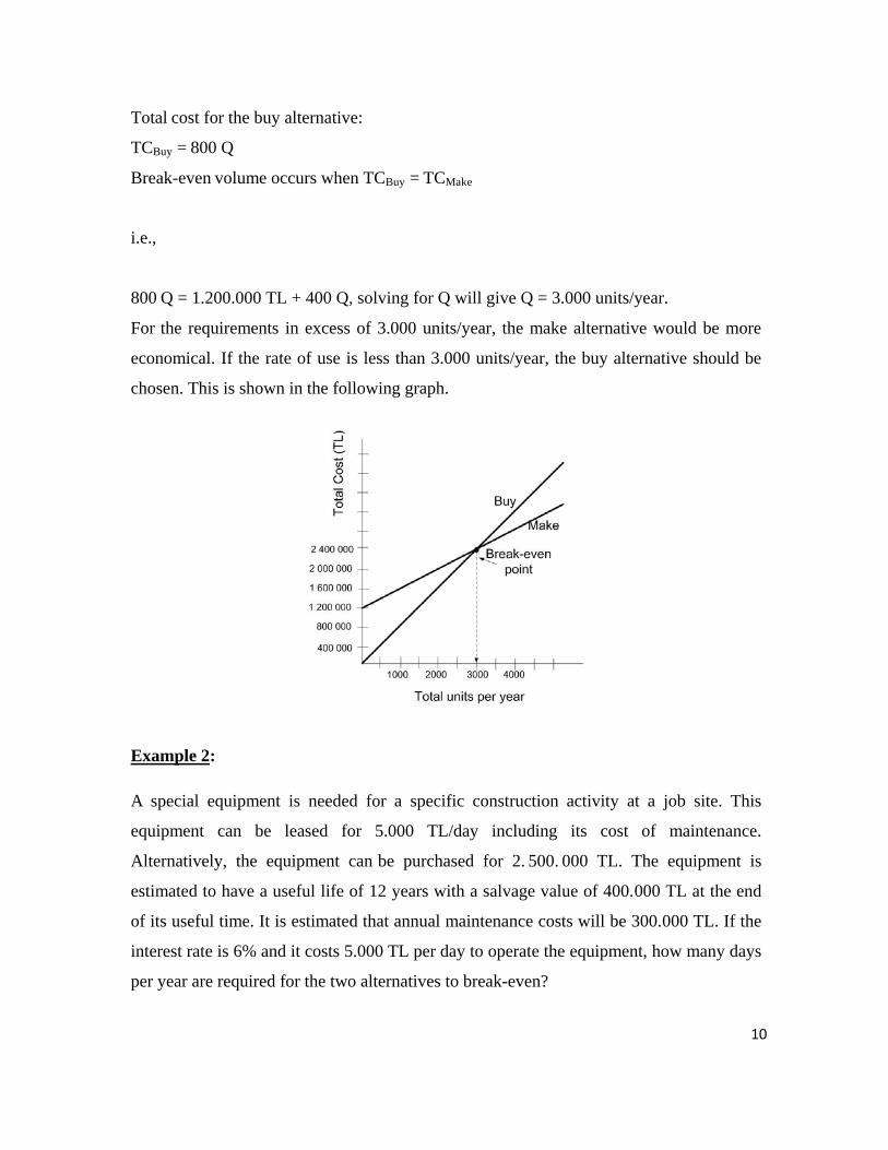
Total cost for the buy alternative:

TCBuy = 800 Q

Break-even volume occurs when TCBuy = TCMake

i.e.,

800 Q = 1.200.000 TL + 400 Q, solving for Q will give Q = 3.000 units/year.

For the requirements in excess of 3.000 units/year, the make alternative would be more

economical. If the rate of use is less than 3.000 units/year, the buy alternative should be

chosen. This is shown in the following graph.

Example 2:

A special equipment is needed for a specific construction activity at a job site. This

equipment can be leased for 5.000 TL/day including its cost of maintenance.

Alternatively, the equipment can be purchased for 2. 500. 000 TL. The equipment is

estimated to have a useful life of 12 years with a salvage value of 400.000 TL at the end

of its useful time. It is estimated that annual maintenance costs will be 300.000 TL. If the

interest rate is 6% and it costs 5.000 TL per day to operate the equipment, how many days

per year are required for the two alternatives to break-even?

11

Solution 2:

Annual costs of the equipment if leased:

TCL = 5.000 Q + 5.000 Q (lease + operation costs)

= 10.000 Q (Q refers to the number of days per year)

Annual costs of the equipment if purchased:

TCP = initial cost – salvage value + maintenance cost + operating costs

TCP = 2.500.000(A/P,6,12) – 400.000(A/F,6,12) + 300.000 + 5.000 Q

TCP = 2.500.000 x 0,1193 – 400.000 x 0,0593 + 300.000 + 5.000 Q

TCP = 298.250 – 23.720 + 300.000 + 5.000 Q

TCP = 574.30 + 5.000 Q

Break-even occurs when TCL= TCP

10.000 Q = 574.530 + 5.000 Q

Q = 115 days/year

For all the levels of use exceeding 115 days/year it would be more economical to

purchase the equipment. If the level of use is anticipated to be below 115 days/year, the

computer should be leased, as shown in the following graph.

12

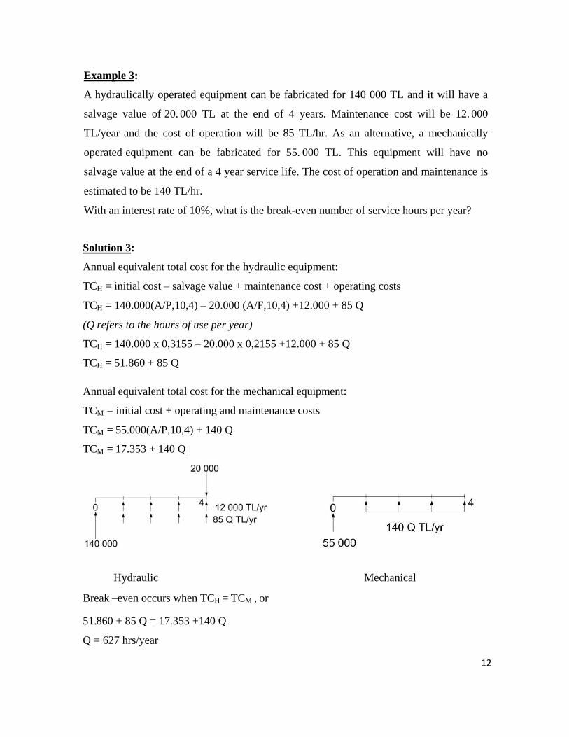
Example 3:

A hydraulically operated equipment can be fabricated for 140 000 TL and it will have a

salvage value of 20. 000 TL at the end of 4 years. Maintenance cost will be 12. 000

TL/year and the cost of operation will be 85 TL/hr. As an alternative, a mechanically

operated equipment can be fabricated for 55. 000 TL. This equipment will have no

salvage value at the end of a 4 year service life. The cost of operation and maintenance is

estimated to be 140 TL/hr.

With an interest rate of 10%, what is the break-even number of service hours per year?

Solution 3:

Annual equivalent total cost for the hydraulic equipment:

TCH = initial cost – salvage value + maintenance cost + operating costs

TCH = 140.000(A/P,10,4) – 20.000 (A/F,10,4) +12.000 + 85 Q

(Q refers to the hours of use per year)

TCH = 140.000 x 0,3155 – 20.000 x 0,2155 +12.000 + 85 Q

TCH = 51.860 + 85 Q

Annual equivalent total cost for the mechanical equipment:

TCM = initial cost + operating and maintenance costs

TCM = 55.000(A/P,10,4) + 140 Q

TCM = 17.353 + 140 Q

Hydraulic Mechanical

Break –even occurs when TCH = TCM , or

51.860 + 85 Q = 17.353 +140 Q

Q = 627 hrs/year

13

For rates of use exceeding 627 hrs/yr, the hydraulic equipment would be economical.

However, if it is anticipated that the rate of use will be less than 627 hrs/yr, then the

mechanically operated equipment should be used, as shown in the following graph.

Example 4:

A company manufacturing prefabricated reinforced concrete building elements is

operating with an annual cost of 40.000.000 TL, a revenue (income) of 1.100 TL/element,

and a variable cost of 600 TL/element. The company hopes to produce 100.000 elements

per year. What is the break-even point? Would the company make a profit or loss?

Assuming that the market is ready for an increase in selling price to 1.600 TL/element,

how would this affect the yearly profit?

Solution 4:

Break-even point occurs when;

Revenue = Cost

1.100 Q = 40.000.000 + 600 Q, where Q is the total elements sold in a year.

Q = 80.000 elements/year

If 100.000 elements per year are made and sold, then annual profit will be;

Profit = Revenue – Cost

14

Profit = 1.100 x 100.000 – 600 x 100.000 – 40.000.000

P = 10.000.000 TL/yr

If selling price is increased from 1.100 TL/element to 1.600 TL/element, then annual

profit will be:

P = (1.600 – 600) x 100.000 – 40.000.000

P = 60.000.000 TL/yr

In other words, if the selling price is increased about 40 to 50%, the annual profit

increases by 600%.

Example 5:

The company in Example 4 is considering usage of a new production equipment which

will save 3.000.000 TL/year in supervision and related fixed costs. With a revenue of

1.100 TL/element, and a variable cost of 600 TL/element, at what volume of production

the company starts making profit? What is the expected profit per year for 100.000 units

of expected production?

Solution 5:

Revenue = Cost

1.100 Q = 40.000.000 – 3.000.000 + 600 Q (Q refers to the number of elements per year)

500 Q = 37.000.000

Q = 74.000 elements/yr

At 100.000 elements per year, the profit will be;

P = (1.100- 600) x 100.000 – (40.000.000 – 3.000.000)

P = 13.000.000 TL/yr which is greater than 10.000.000 TL/yr when the fixed cost was

40.000.000 TL/yr.

15

Example 6:

The company in example 4 considers an advertisement campaign which will make it

possible to sell elements for 1.125 TL/element. What is the new volume of production at

which revenues will be equal to costs? What will annual profits become? How much can

the company spend on the advertisement campaign?

Solution 6:

Break even volume will be at:

40.000.000 + 600 Q = 1.125 Q (Q refers to the number of elements per year)

Q = 76.190 elements/yr

At 100.000 elements per year, profits will be:

P = (1.125-600) x 100.000 – 40.000.000

P = 12.500.000 TL/yr > 10.000.000 TL/yr when the selling price was 1.100

TL/element. The company can spend for the advertisement:

12.500.000 – 10.000.000 = 2.500.000 TL/yr.

Example 7:

A toy company currently purchases the metal parts which are required in the manufacture

of certain toys, but there has been a proposal that the company make these parts themselves.

Two machines will be required for the operation: Machine A will cost 18.000 TL, have a

life of six years, and a 2.000 TL salvage value; Machine B will cost 12.000 TL, have a life

of four years, and a -500 TL salvage value. Machine A will require an overhaul after three

years costing 3.000 TL. The annual operating cost of Machine A is expected to be 6.000

per year and for Machine B 5.000 TL per year. A total of four laborers will be required for

the two machines at a cost of 2,50 TL per hour per worker. In a normal eight-hour day, the

machines can produce parts sufficient to manufacture 1.000 toys. If the company’s present

price for these parts is 0,50 TL per toy, how many toys must be manufactured each year in

order to justify the purchase of the machines? Use a MARR of 15% per year.

16

Solution 7:

Variable cost/year = (cost/unit)(unit/year) = xx 08,0000.1

)8)(50,2(4

Where x = number of units per year

For Machine A, the fixed costs per year:

AEA = 18.000 (A/P,15%,6) – 2.000 (A/F,15%,6) + 6.000

+ 3.000(P/F,15%,3)(A/P,15%,6)

AEA = 18.000*0,2642 – 2.000*0,1142 + 6.000 + 3.000*0,6575*0,2642

AEA = 11.048 TL

For Machine B, the fixed costs per year:

AEB = 12.000 (A/P,15%,4) +500 (A/F,15%,4) + 5.000

AEB = 12.000*0,3503 + 500*0,2003 + 5.000

AEB = 9.304 TL

Equating the annual costs of the purchase option (0,50x) and the manufacture option:

0,50x = 11.048 +9.304 + 0,08x

0,42x = 20.352

x = 48.457 units

Example 8:

A construction company is planning to convert a plant from manufacturing steel

components for railways (lines, axes, etc.) to manufacturing for buildings (beams, columns,

etc.) The initial cost for equipment conversion will be 60 million TL with a 15% salvage

value anytime within a 7-year period. The cost of producing each component will be 100

TL, and they will be sold for 250 TL. The production capacity for the first year will be

50.000 components. At a MARR of 9% per year, by what uniform amount will production

have to increase each year in order for the company to recover its investment in 4 years?

Solution 8:

Let X = gradient increase per year

Total costs =

-60.000.000 (A/P,9%,4) + (0,15)(60.000.000)(A/F,9%,4) – [50.000 + X (A/G,9%,4)](100)

Revenue = [50.000 + X (A/G,9%,4)](250)

17

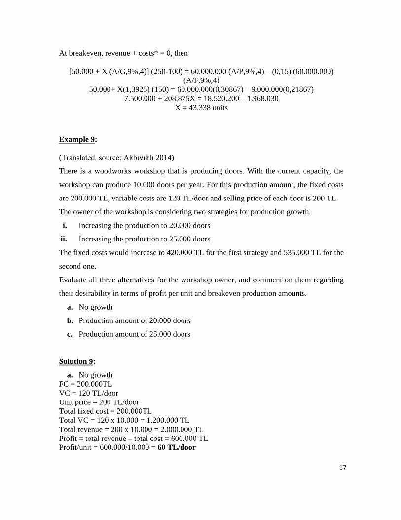
At breakeven, revenue + costs* = 0, then

[50.000 + X (A/G,9%,4)] (250-100) = 60.000.000 (A/P,9%,4) – (0,15) (60.000.000)

(A/F,9%,4)

50,000+ X(1,3925) (150) = 60.000.000(0,30867) – 9.000.000(0,21867)

7.500.000 + 208,875X = 18.520.200 – 1.968.030

X = 43.338 units

Example 9:

(Translated, source: Akbıyıklı 2014)

There is a woodworks workshop that is producing doors. With the current capacity, the

workshop can produce 10.000 doors per year. For this production amount, the fixed costs

are 200.000 TL, variable costs are 120 TL/door and selling price of each door is 200 TL.

The owner of the workshop is considering two strategies for production growth:

i. Increasing the production to 20.000 doors

ii. Increasing the production to 25.000 doors

The fixed costs would increase to 420.000 TL for the first strategy and 535.000 TL for the

second one.

Evaluate all three alternatives for the workshop owner, and comment on them regarding

their desirability in terms of profit per unit and breakeven production amounts.

a. No growth

b. Production amount of 20.000 doors

c. Production amount of 25.000 doors

Solution 9:

a. No growth

FC = 200.000TL

VC = 120 TL/door

Unit price = 200 TL/door

Total fixed cost = 200.000TL

Total VC = 120 x 10.000 = 1.200.000 TL

Total revenue = 200 x 10.000 = 2.000.000 TL

Profit = total revenue – total cost = 600.000 TL

Profit/unit = 600.000/10.000 = 60 TL/door

18



Total VC = 120 x 20.000 = 2.400.000 TL


Profit = total revenue – total cost = 1.180.000 TL

Profit/unit = 1.180.000/20.000 = 59 TL/door



Total VC = 120 x 25.000 = 3.000.000 TL


Profit = total revenue – total cost = 1.465.000 TL

Profit/unit = 1.465.000/25.000 = 58,6 TL/door

Breakeven amounts for each alternative:

a. No growth

Q = 200.000 / (200-120) = 2.500 doors


Q = 420.000 / (200-120) = 5.250 doors


Q = 535.000 / (200-120) = 6.688 doors

Profitability is decreasing as the capacity and revenue increases.

Example 10:

A product currently sells for 20 TL per unit. The variable costs are 8 TL/unit, and this

specific design (Design A) sells 10.000 units annually with a profit of 40.000 TL acquired

per year. The company is trying to make a 10-year plan to decide if any improvements are

can be initiated for the production line. As an initial idea, company is considering to change

the existing design of the product. This new design (Design B) will increase the variable

costs by 25% and fixed costs by 10% for this production machine (Machine I). Sales are

forecasted to increase 2.500 units per year with Design B. Alternatively, without changing

the design of the product (using Design A), the company can change the production

machine (Machine II) for 43.625 TL initial cost, no salvage value, and additional annual

maintenance cost of 5.000 TL. The variable costs are expected to be 8 TL/unit in that case.

The last alternative is integrating Design B with Machine II, then the associated variable

cost will be 10 TL/unit. MARR is 10%. Given this information please answer the following

questions:

19

a. If the company decides to go with Design B, at what selling price does this alternative

break-even?

b. If the selling price is to be kept same (20 TL/unit) what will the annual profit be for

the design update (Machine I, Design B)?

c. For the new machine, the selling quantities are estimated as 13.500 units for Design

A and 15.000 units for Design B. If the selling price is kept the same, which

alternative should be selected as the 10-year investment plan?

d. If 12.000 products will be produced annually, please calculate the selling price for

each of these alternatives separately so that each of them breaks-even individually.

Solution 10:

Profit = revenue – costs

40.000 = 10.000(20) – [10.000(8) + FC] FC = 80.000 TL

Design change:

New variable cost = 8(1,25) = 10 TL/unit

New fixed costs = 80.000(1,1) = 88.000 TL

a. Breakeven analyses for Design B

Let X = breakeven selling price per unit, then

12.500X = 88.000 + 12.500(10)

X = 17,04 TL/unit

b. Profit analysis for Design B

Profit = 12.500(20) – 12.500(10) – 88.000 = 37.000 TL

c. New machine, Design A

FC = 43.625(A/P, 10%, 10) + 5.000 + 80.000

FC = 43.625*0,16275 + 85.000 = 92.100 TL

Profit = 20*13.500 – 8*13.500 – 92.100 = 69.900 TL

New Machine, Design B

FC = 43.625 (A/P, 10%, 10) + 5.000 + 88.000

FC = 43.625*0,16275 + 93.000 = 100.100 TL

Profit = 20*15.000 – 10*15.000 – 100.100 = 49.900 TL

New Machine, Design A should be selected.

d. Machine 1, Design A: 12.000X = 80.000 + 12.000*8 X = 14,67 TL/unit

Machine 1, Design B: 12.000X = 88.000 + 12,000*10 X = 17,33 TL/unit

Machine 2, Design A: 12.000X = 92.100 + 12.000*8 X = 15,68 TL/unit

Machine 2, Design B: 12.000X = 100.100 + 12.000*10 X= 18,34 TL/unit

20

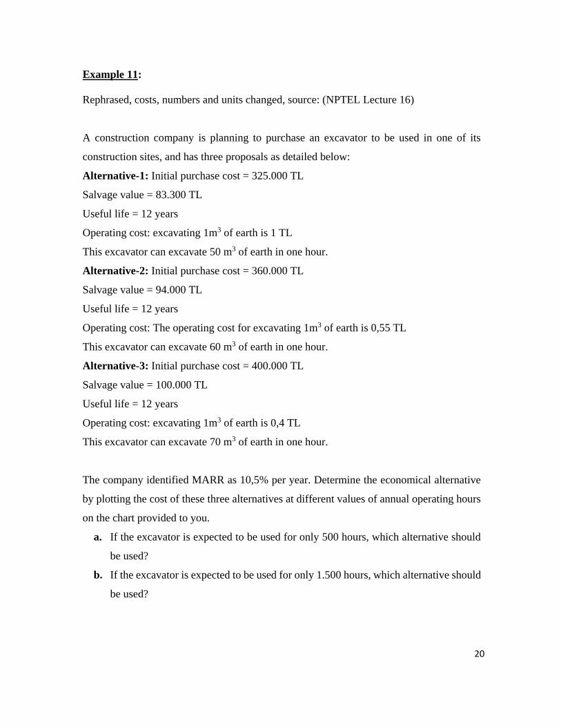
Example 11:

Rephrased, costs, numbers and units changed, source: (NPTEL Lecture 16)

A construction company is planning to purchase an excavator to be used in one of its

construction sites, and has three proposals as detailed below:

Alternative-1: Initial purchase cost = 325.000 TL

Salvage value = 83.300 TL

Useful life = 12 years

Operating cost: excavating 1m3 of earth is 1 TL

This excavator can excavate 50 m3 of earth in one hour.




Operating cost: The operating cost for excavating 1m3 of earth is 0,55 TL





Operating cost: excavating 1m3 of earth is 0,4 TL


The company identified MARR as 10,5% per year. Determine the economical alternative

by plotting the cost of these three alternatives at different values of annual operating hours

on the chart provided to you.

a. If the excavator is expected to be used for only 500 hours, which alternative should

be used?

b. If the excavator is expected to be used for only 1.500 hours, which alternative should

be used?

21

Solution 11:

Pair-wise comparison between the alternatives is performed to determine the breakeven

point.

Let ‘X’ be the number of operating hours per year.

Annual operating cost (TL) for Alternative-1:

1 TL/m3 * 50 m3/hr * X hr/year = 50X TL/year

AEAlternative-1:

AE1 = -325.000 (A/P, 10,5%, 12) – 50X + 83,300 (A/F, 10,5%, 12)

AE1 = -325.000* 0,1504 – 50X + 83.300* 0,0454 = -45.098 – 50X


0,55 TL/m3 * 60 m3/hr * X hr/year = 33X TL/year

AEAlternative-2:

AE2 = -360,000(A/P, 10,5%, 12) –3X + 94,000 (A/F, 10,5%, 12)

AE2 = -360.000*0,1504 – 33X + 94.000* 0,0454 = -49.876 – 33X


0,4TL/m3 * 70 m3/hr * X hr/year = 28X TL/year

AEAlternative-3:

AE3 = -400.000 (A/P, 10,5%, 12) – 28X + 100.000 (A/F, 10,5%, 12)

AE3 = -400.000* 0,1504 – 28X + 100.000* 0,0454 = -55,620 – 28X

The equivalent uniform annual

worth (cost) of all the

alternatives are determined at

different values of annual

operating hours and are shown

in the figure.

AE1 = AE2

-45.098 – 50X = -49.876 – 33X

X = 281 hours/year

AE1 = AE3

-45.098 – 50X = -55.620 – 28X

X = 478 hours/year

AE2 = AE3

-49.876 – 33X = -55.620 – 28X

X = 1.149 hours/year

22

Alternative-1 should be selected, if the expected annual operating hours are less than the

281 hours, Alternative-2 should be selected, if the expected annual operating hours are

between 281 and 1.149 hours. Alternative-3 should be selected, if the expected annual

operating hours are greater than 1.149 hours.

a. Alternative 2 should be selected.

b. Alternative 3 should be selected.

Example 12:

An investor is going to get a multi-story apartment constructed. They have four alternatives

as building materials: steel, concrete, stone masonry or brick. The costs associated with

each alternative is presented in the following table. Please carry out breakeven analyses to

determine which material should be used for what ranges of building area so that cheapest

alternative is selected. In your calculations, consider MARR as 15% per year and plot your

findings on the chart.

Steel Concrete Stone

Masonry Brick

Initial cost 30 TL/m2 20 TL/m2 32 TL/m2 25 TL/m2

Maintenance 40.000

TL/year

25.000

TL/year

15.000

TL/year

18.000

TL/year

Heating 1 TL/m2/year 1,5

TL/m2/year

2,2

TL/m2/year 2 TL/m2/year

Salvage

Value

75% of initial

cost

90% of initial

cost

100% of

initial cost

100% of

initial cost

Life span 25 years 25 years 25 years 25 years

Solution 12:

Let X = area in m2

Using AE values:

AES = -(30X)(A/P,15%,25) + (0,75)(30X)(A/F,15%,25) – 40.000 –X

= -(30X)(0,15470) + (0,75)(30X)(0,00470) – 40.000 –X

= -4,641X + 0,10575X – 40.000 – X

= -5,535X – 40.000

AEC = -(20X)(A/P,15%,25) + (0,9)(20X)(A/F,15%,25) – 25.000 – 1,5x

= -(20X)(0,15470) + (0,9)(20X)(0,00470) – 25.000 – 1,5x

= -3,094X + 0,0846X – 25.000 – 1,5X

= -4,509X – 25.000

23

AESM = -(32X)(A/P,15%,25) + (1,0)(32X)(A/F,15%,25) – 15.000 – 2,2X

= -(32X)(0,15470) + (1,0)(32X)(0,00470) – 15.000 – 2,2X

= -4,950X + 0,1504X – 15.000 – 2,2X

= -7X – 15.000

AEB = -(25X)(A/P,15%,25) + (1,0)(25X)(A/F,15%,25) – 18.000 – 2X

= -(25X)( 0,15470) + (1,0)(25X)( 0,00470) – 18.000 – 2X

= -3,8675X + 0,1175X – 18.000 – 2X

= -5,75X – 18.000

Breakeven Analyses:

Steel vs Concrete:

-5,535X – 40.000 = -4,509X – 25.000

X < 0 negative

Steel vs Brick:

-5,535X – 40.000 = -5,75X – 18.000

x =102.326 m2

Steel vs Stone Masonry

-5,535X – 40.000 = -7X – 15.000

x= 17.065 m2

Concrete vs Brick:

-4,509X – 25.000 = -5,75X – 18.000

x= 5.641 m2

Concrete vs Stone Masonry

-4,509X – 25.000 = -7X – 15.000

x= 4.015 m2

Brick vs Stone Masonry

-5.750x -18,000 = -7X – 15.000

x= 2.400 m2

for X < 2.400 stone

for 2.400 < X < 5.641 brick

for X > 5.641 concrete

Following examples are adapted from Lecture Notes provided by Department of Industrial

Engineering, Eastern Mediterranean University (“EMU”).

0

20000

40000

60000

80000

100000

120000

140000

160000

180000

0 5000 10000 15000 20000 25000

steel concrete stone brick

24

Example 13:

The ABC Company is faced with three alternatives for their fabrication work. Alternative

A involves the purchase of a machine for 5.000 TL. It will have a seven-year life, with a

zero salvage value at that time. Alternative A involves additional costs of TL0,20 per unit

of product produced per year. Alternative B involves the purchase of a machine for 10.000

TL. It will also have a seven-year life, with 2.000 TL salvage value at that time. Alternative

B involves additional costs of 0,15 TL per unit of product produced per year. Alternative C

involves the purchase of a machine for 8.000 TL. It will have a 2.000 TL salvage value

when disposed of in seven years. Additional costs of 0,25 TL per unit of product per year

arise when Alternative C is used. An 8% interest rate is used by the ABC Company in

evaluating investment alternatives. For what range of annual production volume values is

each method preferred?

Solution 13:

Let X = number of units per year

AEA = -5.000 (A/P,8%,7) – 0,2X = -5.000 (0,19207) – 0,2X

AEA = -960,35 – 0,2X

AEB = -10.000(A/P,8%,7) + 2.000(A/F,8%,7) – 0,15X = -10.000(0,19207) +

2.000(0,11207) – 0,15X

AEB = -1.696,56 – 0,15X

AEC = -8.000(A/P,8%,7) + 2.000(A/F,8%,7) – 0,25X

AEC = -1.312,42 – 0,25X

A vs B: -960,35 – 0,2X = -1.696,56 – 0,15X

XAB = 14.724,2

B vs C: -1.696,56 – 0,15X = -1.312,42 – 0,25X

XBC = 3.841,4

A vs C: No intersection for X > 0.

25

C A B

Total Cost

4.000

X 14.724, select A

X > 14.724, select B

2.000

X

3.841 10.000 14.724 20.000

Number of units per year

Alternative solution (without graph):

Check minimum cost at each unit interval by picking random values at each interval (break

even points represent the points of possible change in cost trend).

Units 3000 10000 16000

CA -1.560,35 TL -2.960,35 TL -4.160,35 TL

CB -2.146,96 TL -3.196,56 TL -4.096,56 TL

CC -2.062,42 TL -3.812,42 TL -5.312,42 TL

Therefore Select A for units<14.724, Select B for units>14.724.

Example 14:

Three types of design proposals for a commercial one - storey building is to be evaluated

details given below:

0 3.841 14.724

3.000 10.000 16.000

26

STEEL CONCRETE BRICK

First cost 72 TL/m2 76 TL/m2 81 TL/m2

Annual maintenance 14.000 TL 9.000 TL 6.000 TL

Annual heating cost 3 TL/m2 3,4 TL/m2 3,9 TL/m2

SV (%of first cost) %80 %100 %110

Life (years) 20 20 20

For what range of building area (m2) which type of design is the most suitable (cheapest) to

select? Carry out break-even analysis using an interest rate of %18 per year and plot your

ranges to illustrate.

Solution 14:

Let X = area in m2

First cost of steel = 72x and its salvage value = (0,8)72x

Using AE values:

AES = -(72x)(A/P,18%,20) + (0,8)(72x)(A/F,18%,20) – 14.000 – 3x

AES = -(72x)(0,18682) + (0,8)(72x)(0,00682) – 14.000 – 3x

AES = -16,058x – 14.000

Similarly,

AEC = -(76x)(A/P,18%,20) + (1,0)(76x)(A/F,18%,20) – 9.000 – 3,4x

AEC = -(76x)(0,18682) + (1,0)(76x)(0,00682) – 9.000 – 3,4x

AEC = -17,08x – 9.000

AEB = -(81x)(A/P,18%,20) + (1,1)(81x)(A/F,18%,20) – 6.000 – 3,9x

AEB = -(81x)(0,18682) + (1,1)(81x)(0,00682) – 6.000 – 3,9x

AEB = -18,425x – 6.000

Break-evens:

Steel vs Concrete:

-16,058x – 14.000 = -17,08x – 9.000

x = 4.892 m2

Steel vs Brick:

-16,058x – 14.000 = -18,425x – 6.000

x = 3.380 m2

Concrete vs Brick:

-17,08x – 9.000 = -18,425x – 6.000

x = 2.231 m2

27

B 0 < x 2.231 Select Brick

C 2.231 < x 4.892 Select Concrete

Total Cost x > 4.892 Select Steel

S

2.231 3.380 4.892

Area, m2


Check minimum cost at each area interval by picking random values at each interval (break

even points represent the points of possible change in cost trend).

Area (m2) 1.000 3.000 4.000 6.000

CSTEEL -30.058 TL -62.174 TL -78.232 TL -110.348 TL

CCONCRETE -26.080 TL -60.240 TL -77.320 TL -111.480 TL

CBRICK -24.425 TL -61.275 TL -79.700 TL -116.550 TL

Therefore, Select Brick for area<2.231 m2, Select Concrete for 2.231 m2<area<4.892 m2,

and Select Steel for area>4.892 m2.

Example 15:

Three options are considered for an engine part:

A – complete in-house manufacturing, with initial equipment cost of 50.000 TL, labor cost

of 26.000 TL per year, and material cost of 10 TL per engine part.

B – partial manufacture, (i.e. partially finished engine parts are purchased), with initial

equipment cost of 35.000 TL, labor cost of 10.000 TL per year, material cost of 3 TL per

engine part, and an additional cost of 40 TL per the partially finished engine part.

C – purchase from outside at a cost of 120 TL per engine part.

Any equipment purchased will have a life of 6 years. If the MARR is 10% per year,

0 2.231 3.380 4.892

1.000 3.000 4.000 6.000

28

determine the number of engine parts that must be manufactured to justify (a) complete in-

house manufacture and (b) partial manufacture. (c) Plot the total cost lines for all three

options, and state the ranges of engine parts for which each option will have the lowest cost.

Solution 15:

Let x = number of engine parts per year.

Using AE values:

AEIN = -50.000(A/P,10%,6) – 26.000 – 10x = -50.000(0,22961) – 26.000 – 10x =

- 37.480,5 – 10x

AEPM = -35.000(A/P,10%,6) – 10.000 – 3x – 40x = -35.000(0,22961)– 10.000– 43x

= - 18.036,35 - 43x

AEOUT = -120x

(a) Complete in-house manufacturing vs purchase from outside:

AEIN = AEOUT

or, -37.480,5 - 10x = -120x

x = 341 parts per year

(b) Partial manufacture vs purchase from outside:

AEPM = AEOUT

-18.036,35 - 43x = -120x

x = 234 parts per year

(c) Complete in-house vs partial manufacture

AEIN = AEPM

-37.480,5 - 10x = -18.036,35 - 43x

x = 589 parts per year from outside

Ranges for the lowest total cost are: partial

Total

0 < x 234 select purchase from outside cost in-house

234 < x 589 select partial manufacture

589 < x select in-house manufacture

234 341 589

Number of engine parts

29


Check minimum cost at each engine parts interval by picking random values at each interval

(break even points represent the points of possible change in cost trend).

Parts 200 300 400 600

CIN -39.480,50 TL -40.480,50 TL -41.480,50 TL -43.480,50 TL

CPM -26.636,35 TL -30.936,35 TL -35.236,35 TL -43.836,35 TL

COUT -24.000,00 TL -36.000,00 TL -48.000,00 TL -72.000,00 TL

Therefore, Select Purchase from Outside for engine parts<234, Select Partial Manufacture

for engine parts 234<area<589, and Select In-House Manufacture for Engine Parts>589.

References:

Akbıyıklı, R. (2014). Mühendislik Ekonomisi: Temel Prensipleri ve Uygulamaları, Birsen Yayınevi,

İstanbul.

Badiru, A. B. (1996). Project Management in Manufacturing and High Technology Operations,

Wiley-IEEE, USA.

Blank, L. T., and Tarquin, A. J. (2008). Engineering Economy, 5th Edition, McGraw-Hill, USA.

Eastern Mediterranean University, Lecture Notes of Industrial Engineering, retrieved on 22nd

February 2014, from http://ie.emu.edu.tr/development/dosyalar/{o2M-or_-Mco}Break.doc

Massachusetts Institute of Technology, OpenCourseWare, 2006 Lecture Notes of 1.011 Project

Evaluation Course.

NPTEL Lecture 16, Lecture Notes on Breakeven analysis for two and more than two alternatives,

retrieved on 3rd January 2017, from http://nptel.ac.in/courses/105103023/33

Paek, J. H. (2000). “Running a profitable construction company: Revisited break-even analysis.”

Journal of Management in Engineering, 16(3), 40-46.

Tockey, S. (2004). Return on Software: Maximizing the Return on Your Software Investment,

Addison-Wesley Professional, USA.

0 234 341 589

200 300 400 600

http://ie.emu.edu.tr/development/dosyalar/%7bo2M-or_-Mco%7dBreak.doc

http://nptel.ac.in/courses/105103023/33

CE 231 ENGINEERING ECONOMY BREAK-EVEN...

Documents

Transcript of CE 231 ENGINEERING ECONOMY BREAK-EVEN...