CDVine: An R-package for statistical inference of C- … An R-package for statistical inference of...
50
CDVine: An R-package for statistical inference of C- and D-vines Ulf Schepsmeier & Eike Christian Brechmann Technische Universit¨ at M¨ unchen May 11, 2011 Schepsmeier & Brechmann (TUM) The R-package CDVine May 11, 2011 1 / 16
Transcript of CDVine: An R-package for statistical inference of C- … An R-package for statistical inference of...
CDVine: An R-package for statistical inferenceof C- and D-vines
Ulf Schepsmeier & Eike Christian Brechmann
Technische Universitat Munchen
May 11, 2011
Schepsmeier & Brechmann (TUM) The R-package CDVine May 11, 2011 1 / 16
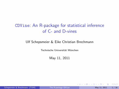
Available software for vines
In general...
I “Uncertainty analysis with Correlations” (UNICORN, TU Delft)includes some functionality for vines.
In R...
I Packages for bivariate and multivariate copulas (copula, fCopulae,QRMlib, nacopula,...), but nothing regarding vines.
I Daniel Berg (U Oslo/NR): copulaGOF/CopulaLib.
The package CDVine fills this gap!
Schepsmeier & Brechmann (TUM) The R-package CDVine May 11, 2011 2 / 16
Scope of CDVine
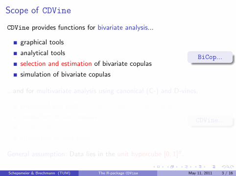
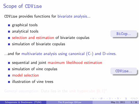
CDVine provides functions for bivariate analysis...
graphical tools
analytical tools
selection and estimation of bivariate copulas
simulation of bivariate copulas
BiCop...
...and for multivariate analysis using canonical (C-) and D-vines.
sequential and joint maximum likelihood estimation
simulation of vine copulas
model selection
illustration of vine trees
p
CDVine...
p
General assumption: Data lies in the unit hypercube [0, 1]d .
Schepsmeier & Brechmann (TUM) The R-package CDVine May 11, 2011 3 / 16
Scope of CDVine
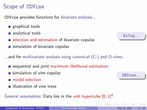
CDVine provides functions for bivariate analysis...
graphical tools
analytical tools
selection and estimation of bivariate copulas
simulation of bivariate copulas
BiCop...
...and for multivariate analysis using canonical (C-) and D-vines.
sequential and joint maximum likelihood estimation
simulation of vine copulas
model selection
illustration of vine trees
p
CDVine...
p
General assumption: Data lies in the unit hypercube [0, 1]d .
Schepsmeier & Brechmann (TUM) The R-package CDVine May 11, 2011 3 / 16
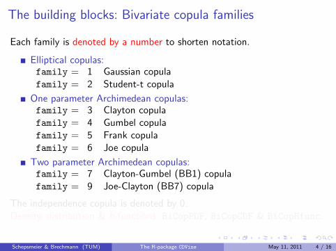
The building blocks: Bivariate copula families
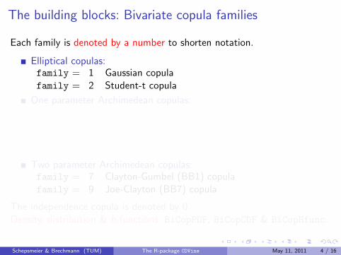
Each family is denoted by a number to shorten notation.
Elliptical copulas:family =
0
1 Gaussian copulafamily =
0
2 Student-t copula
One parameter Archimedean copulas:
Two parameter Archimedean copulas:family =
0
7 Clayton-Gumbel (BB1) copulafamily =
0
9 Joe-Clayton (BB7) copula
The independence copula is denoted by 0.Density, distribution & h-functions: BiCopPDF, BiCopCDF & BiCopHfunc.
Schepsmeier & Brechmann (TUM) The R-package CDVine May 11, 2011 4 / 16
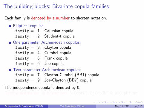
The building blocks: Bivariate copula families
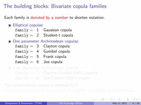
Each family is denoted by a number to shorten notation.
Elliptical copulas:family =
0
1 Gaussian copulafamily =
0
2 Student-t copula
One parameter Archimedean copulas:family =
0
3 Clayton copulafamily =
0
4 Gumbel copulafamily =
0
5 Frank copulafamily =
0
6 Joe copula
Two parameter Archimedean copulas:family =
0
7 Clayton-Gumbel (BB1) copulafamily =
0
9 Joe-Clayton (BB7) copula
The independence copula is denoted by 0.Density, distribution & h-functions: BiCopPDF, BiCopCDF & BiCopHfunc.
Schepsmeier & Brechmann (TUM) The R-package CDVine May 11, 2011 4 / 16
The building blocks: Bivariate copula families
Each family is denoted by a number to shorten notation.
Elliptical copulas:family =
0
1 Gaussian copulafamily =
0
2 Student-t copula
One parameter Archimedean copulas:family =
0
3 Clayton copulafamily =
0
4 Gumbel copulafamily =
0
5 Frank copulafamily =
0
6 Joe copula
Two parameter Archimedean copulas:family =
0
7 Clayton-Gumbel (BB1) copulafamily =
0
9 Joe-Clayton (BB7) copula
The independence copula is denoted by 0.Density, distribution & h-functions: BiCopPDF, BiCopCDF & BiCopHfunc.
Schepsmeier & Brechmann (TUM) The R-package CDVine May 11, 2011 4 / 16
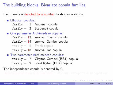
The building blocks: Bivariate copula families
Each family is denoted by a number to shorten notation.
Elliptical copulas:family =
0
1 Gaussian copulafamily =
0
2 Student-t copula
One parameter Archimedean copulas:family = 13 survival Clayton copulafamily = 14 survival Gumbel copulafamily =
0
5 Frank copulafamily = 16 survival Joe copula
Two parameter Archimedean copulas:family =
0
7 Clayton-Gumbel (BB1) copulafamily =
0
9 Joe-Clayton (BB7) copula
The independence copula is denoted by 0.Density, distribution & h-functions: BiCopPDF, BiCopCDF & BiCopHfunc.
Schepsmeier & Brechmann (TUM) The R-package CDVine May 11, 2011 4 / 16
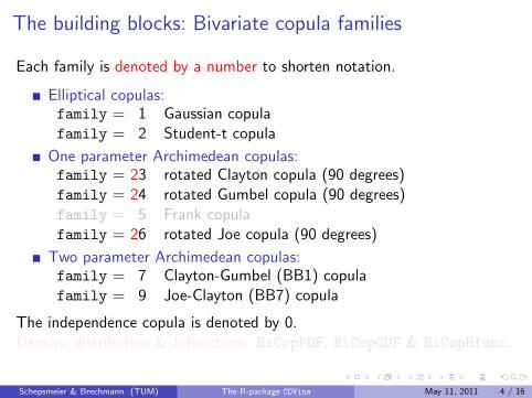
The building blocks: Bivariate copula families
Each family is denoted by a number to shorten notation.
Elliptical copulas:family =
0
1 Gaussian copulafamily =
0
2 Student-t copula
One parameter Archimedean copulas:family = 23 rotated Clayton copula (90 degrees)family = 24 rotated Gumbel copula (90 degrees)family =
0
5 Frank copulafamily = 26 rotated Joe copula (90 degrees)
Two parameter Archimedean copulas:family =
0
7 Clayton-Gumbel (BB1) copulafamily =
0
9 Joe-Clayton (BB7) copula
The independence copula is denoted by 0.Density, distribution & h-functions: BiCopPDF, BiCopCDF & BiCopHfunc.
Schepsmeier & Brechmann (TUM) The R-package CDVine May 11, 2011 4 / 16
The building blocks: Bivariate copula families
Each family is denoted by a number to shorten notation.
Elliptical copulas:family =
0
1 Gaussian copulafamily =
0
2 Student-t copula
One parameter Archimedean copulas:family = 33 rotated Clayton copula (270 degrees)family = 34 rotated Gumbel copula (270 degrees)family =
0
5 Frank copulafamily = 36 rotated Joe copula (270 degrees)
Two parameter Archimedean copulas:family =
0
7 Clayton-Gumbel (BB1) copulafamily =
0
9 Joe-Clayton (BB7) copula
The independence copula is denoted by 0.Density, distribution & h-functions: BiCopPDF, BiCopCDF & BiCopHfunc.
Schepsmeier & Brechmann (TUM) The R-package CDVine May 11, 2011 4 / 16
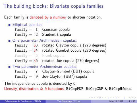
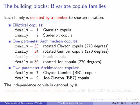
Rotation of copulas
I Rotate asymmetric Archimedean copulas to capture negativedependence: if (U1,U2) ∼ C90◦ , then (1− U1,U2) ∼ C0◦ .
I Survival copulas correspond to rotation by 180 degrees.
Clayton copulas rotated by 0, 90, 180 and 270 degrees
> dat0 = BiCopSim(N = 500, family = 3, par = 2)
> dat90 = BiCopSim(N = 500, family = 23, par = -2)
> dat180 = BiCopSim(N = 500, family = 13, par = 2)
> dat270 = BiCopSim(N = 500, family = 33, par = -2)
Schepsmeier & Brechmann (TUM) The R-package CDVine May 11, 2011 5 / 16
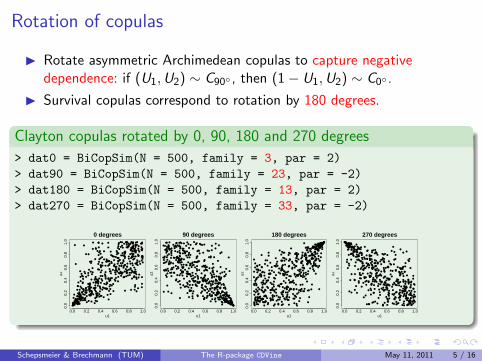
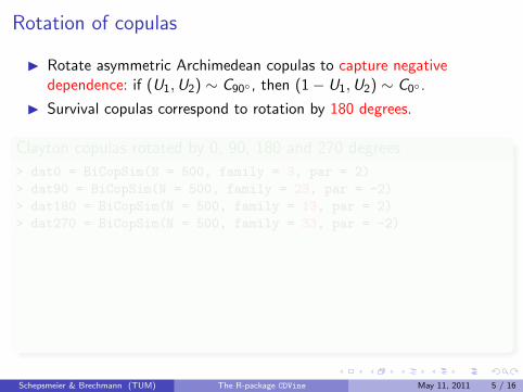
Rotation of copulas
I Rotate asymmetric Archimedean copulas to capture negativedependence: if (U1,U2) ∼ C90◦ , then (1− U1,U2) ∼ C0◦ .
I Survival copulas correspond to rotation by 180 degrees.
Clayton copulas rotated by 0, 90, 180 and 270 degrees
> dat0 = BiCopSim(N = 500, family = 3, par = 2)
> dat90 = BiCopSim(N = 500, family = 23, par = -2)
> dat180 = BiCopSim(N = 500, family = 13, par = 2)
> dat270 = BiCopSim(N = 500, family = 33, par = -2)
●
●
●
●
●
●
●
●
●
●
●
●●
●
●
●
●
●
●
●
●
●
●
●
●
●
●●
●
●
●
●
●
●
●
●
●
●
●
●
●
●
●
●
●
●
●
●
●
●
●
●
●
●
●
●
●
●
●
●
●
●
●
●
●
●
●
●
●
●
●
●
●
●
●
●
●
●
●
●
●
●
●
●
●
●
●
●
●
●
●
●
●
●
●
●
●
●
●
●
●
●
●
●
●
●
●
●
●
●
●
●
●
●
●
● ●●
●
●
●
●
●
●
●
●
●
●
●
●
●●
●
●
●
●
●
●
●
●
●
●
●
●
●
●●
●
●
●
●
●
●
●
●
●
●
●
●●
●
●
●
●
●
●
●
●
●
●
●
●
●
●
●
●
●
●
●
●
●
●
●
●
●
●
●
●
●
●
●
●
●
●
●
●
●
●
●
●
●
●
●
●
●
● ●
●
●
●
●
●
●
●
●
●
●
●
●
●
●
●
●
●
●
●
●
●
●
●
●
●
●
●
●
●
●
●
●
●
●
●
●
●
●
●
●●
●
●
●
●
●●
●
●
●
●
●
●
●●
●
●
●●
●
●
●
●
●
●
●
●
●
●
●
●
●
●
●
●
●
●
●
●
●
●
●
●
●
●
●
●
●●
●
●
●
●
●
●
●
●
●
●
●
●
●
●
●
●
●
●
●
●●
●
●
●
●
●
●
●
●
●
●
●
●
●
●
●
●
●
●
●
●
●
●
● ●
●
●
●
●
●
●
●
●
●
●
●
●
●
●
●
●
●
●
●
●
●
●
●
●●
●
●
●
●
●
●
●
●
●
●
●
●
●
●
●
●
●
●
●●
●
●
●
●
●
●
●
●
●
●
●
●
●
●
●●
●
●
●
●●
●
●
●
●
●
●
●
●
●
●
●●
●
● ●●
●
●
●
●
●
●
●
●
●
●
●
●
●
●
●
●
●
●
●
●
●
●
●
●
●●
●
●
●●
●
●
●
●
●
●
●
●
●
●
●
●
●
●
●
●
●
●
●
●
●
●
●●
●
●
●
●
●
●
●
●
●
●
●
●
●
●
●
●
●
●
●
●
●
●
●
0.0 0.2 0.4 0.6 0.8 1.0
0.0
0.2
0.4
0.6
0.8
1.0
0 degrees
u1
u2
●
●
●●
●
●●
●
●
●
●
●
●
●●
●
●
●
●
●
●
●
●
●
●
●
●
●
●
●
●
●●
●
●
●
●
●
●● ●
●
●
●
●
●
●
●●
●
●
●
●
●
●
●
●
●
●
●
●
●
●
●
●
●
●
●
●
●●
●
●
●
●
●
●
●
●
●
●●
●
●
●
●
●
●
●
●
●
●
●
●
●
●
●
●
●
●
●
●
●
●
●
●
●
●
●
●
●
●
●
●
●
●
●
●
●
●
●
●
●
●
●
●
●
●
●
●
●
●
●
●
●
●
●
●
●
●
●
●
●
●
●
●
●
●
●
●
●
●
●
●
●
●
●
●
●
●
●
●
●
●
●
●
●
●
●
●
●
●
●
●
●
●
●
●
●
●
●
●
●
●
●
●
●
●
●
●
●
●
●
●
●
●
● ●
●
●
●
●
●
●
●
●
●
●
●
●
●
●
●
●
●
●
●
●
●
●
●
●
●
●
●
●
●
●●
●
●●
●
●
●
●
●
●
●
●●
●
●
●
●
●
●
●
●
●
●
●
●
●
●●
●
●
●
●
●
●
●
●
●
●
●
●
●
●
●
●
●
●
●
●
●
●
●
●
●
●
●
●
●
●
●
●
●
●
●
●
●
●
●
●
●
●
●
●
●
●
●
●
●
●
●
●
●
●
●
●
●
●
●
●
●
●
●
●
●
●
●●
●
●
●
●
●
●
●
●
●
●
●
●
●
●
●
●
●
●
●
●
●
●
●
●
●
●
●
●
●
●
●
●
●
●
●
●
●
●
●
●
●
●
●
●
●
●
●
●
●
●
●
●
●
●
●
●
●
●
●
●
●
●
●
●
●
●
●
●
●
●
●
●
●
●
●
●
●
●
●
●
●
●
●
●
●●
●
●
●
●
●
●
●
●
●●
●
●
●
●
●
●
●
●
●
●
●
●
●
●
●
●
●
●●
●
●
●
●
●
●
●
●
●
●
●
●
●
●
●
●
●
●
●
●
●
●
●
●
●
●
●
●
●
●
●
●
●
●
●●
●
●
●
●
●
●●
●
●
●
●
●
●
●
●
●
●
●
●
●
●
●●
●
●
0.0 0.2 0.4 0.6 0.8 1.0
0.0
0.2
0.4
0.6
0.8
1.0
90 degrees
u1
u2
●
●
●
●
●●
●
●
●
●
●
●
●
●
●
●
●
●
●
●
●
●
●
●
●
●
●
●
●
●
●
●
●
●
●● ●
●
● ●
●
●
●
●
●
●
●
●
●
●
●
●
●
●
●
●
●
●
●
●
●
●
●
●
● ●
●
●
●
●
●
●
●
●
●
●
●
●
●
●
●
●
●
●
●
●
●
●●
●
●
●
●
●
●
●
●
●
●
●
●
●
●
●
●
●
●●
●
●
●
●
●
●
●
●
●
●
●●
●
●
●
●
●
●
●
●
●
●
●
●
●
●
●
●
●
●
●
●
●
●
●●
●
●
●
●
●
●
●
●
●
●
●
●
●
●
●
●
●●
●
●
●
●
●
●
●
●
●
●
●
●
●
●
●
●
●
●
●
●
●●
●
●
●
●
●
●
●
●
●
●
●
● ●
●
●
●
●
●
●
●
●
●
●
●
●
●
●
●
●
●
●
●
●
●
●
●
●
●
●
●
●
●
●
●
●●
●
●
● ●
●
●
●
●
●
●
●
●
●
●
●
●
●
●
●
●
●
●
●
●
●
●
●
●
●
●
●
●
●
●
●
●
●
●
●
●
●
●
●
●
●●
●
● ●
●
●
●
●
●
●
●
●
●
●
●
●
●
●
●
●
●●
● ●
●
●
●
●
●
●
●
●
●
●
●
●
●●
●
●
●
●
●
●
●
●
●
●
●●
●
●
●
●
●
●
●
●
●
●
●
●
●
●
●
●
●
●
●
●
●
● ●
●
●
●
●
●
●●
●
●
●
●
●
●
●
● ●
●
●
●
●
●
●
●
●
●
●
●
●
●
●●
●
●
●
●
●
●
●
●
●
●
●
●
●
●
●
●
●
●
●
●
●
●
●
●
●
●
●
●
●
●
●
●
●
●
●
●
●
●
●
●
●
●
●
●
●
●
●●
●
●
●
●
●
●
● ●
●●
●
●
●
●
●
●
●
●
●
●
●
●
●
●
●
●
●
●
●
●
●
●
●
●
●
●
●
●
●
●
●
●
●
●
●
●
●
●
●
●
●
●
●
●
●
●
●
●
●
●
●
●
●
●
●
●
●
●
●
●
●
● ●
0.0 0.2 0.4 0.6 0.8 1.0
0.0
0.2
0.4
0.6
0.8
1.0
180 degrees
u1
u2
●
●
●
●
●
●
●
●
●
●
●
●●
●
●
●
●
●
●
●
●
●
●
●●
●
●
●
●
●
●
●
●
●
●
●
●
●●
●
●●
●
●
●
●
●
●
●
●
●
●
●
●
●
●
●
●
●
●
●
●
●
●
●
●
●
●
●
●
●
●
●
●
●
●
●
●
●
●
●
●
●
●
●
● ●
●
●
●
●
●
●
●
●
●
●
●
●
●
●
●
●
●
●
●
●
●
●●
●
●
●
●
●
●
●
●
●
●
●
●
●
●
●
●
●
●
●
●
●
●
●
●
●
●
●
●
●
●
●
●
●
●
●
●
●
●
●
●
●
●
●
●
●
●
●
●
●
●
●
●
●
●
●
●
●
●
●
●
●
●
●
●
●
●
●
●
●
●
●
●
●
●
●
●
●
●
●
●
●
●
●
●
●
●
●
●
●
●
●
●
●
●
●
●
●
●
●
●●
●
●
●
●
●
●
●
● ● ●●
●
●
●
●
●
●
●
●
●
●●
●
●
●
●
●
●
●
●
●
●
●
●
●●
●
●
●
●
●
●
●
●
●
●
●
●
●
●
●
●
●
●●
●
●
●
●
●
●
●
●●
●
●
●●
●
●
●
●
●
●
●
●
●
●
●
●
●
●
●
●
●
●
●
●
●
●
●
●
●●
● ●●
●
●
●
●
●
●
●
●
●
●
●
●
●
●
●
●
●
●
●
●
●
●
●
●
●
●
●
●
●
●
●
●
●
●
●
●
●
●
●
●
●
●
●
●
●
●
●
●
●
●
●
●
●
●
●
●
●
●●
●
● ●
●
●
●
●
●
●
●
●
●
●
●
●
●
●
●
●
●
●
●
●
●
●
●
●●
●
●
●
●
●
●
●
●
●
●
●
●
●
●
●
●
●
●
●
●
●
●
●
●
●
●
●
●
●
●
●
●
●
●
●
●
●
●
●
●
●
●
●
●
●
●
●
●
●
●
●
●
●
●
●
●
●
●
●
●
●
●
●
●
●
●
●
●
●
●
●
●
●
●
●
●
●
●
●
●
●
●
●
●
●
●
●
●
●
●
●
●
●
●●
●
●●
●
●
●
●
●
●
●
0.0 0.2 0.4 0.6 0.8 1.0
0.0
0.2
0.4
0.6
0.8
1.0
270 degrees
u1
u2
Schepsmeier & Brechmann (TUM) The R-package CDVine May 11, 2011 5 / 16
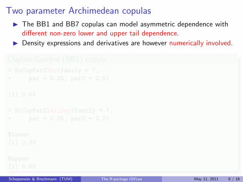
Two parameter Archimedean copulas
I The BB1 and BB7 copulas can model asymmetric dependence withdifferent non-zero lower and upper tail dependence.
I Density expressions and derivatives are however numerically involved.
Clayton-Gumbel (BB1) copula
> BiCopPar2Tau(family = 7,
+ par = 0.25, par2 = 2.5)
[1] 0.64
> BiCopPar2TailDep(family = 7,
+ par = 0.25, par2 = 2.5)
$lower
[1] 0.33
$upper
[1] 0.68
Schepsmeier & Brechmann (TUM) The R-package CDVine May 11, 2011 6 / 16
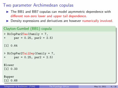
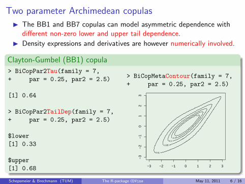
Two parameter Archimedean copulas
I The BB1 and BB7 copulas can model asymmetric dependence withdifferent non-zero lower and upper tail dependence.
I Density expressions and derivatives are however numerically involved.
Clayton-Gumbel (BB1) copula
> BiCopPar2Tau(family = 7,
+ par = 0.25, par2 = 2.5)
[1] 0.64
> BiCopPar2TailDep(family = 7,
+ par = 0.25, par2 = 2.5)
$lower
[1] 0.33
$upper
[1] 0.68
> BiCopMetaContour(family = 7,
+ par = 0.25, par2 = 2.5)
0.01
0.05
0.1 0.15
0.2
−3 −2 −1 0 1 2 3
−3
−2
−1
01
23
Schepsmeier & Brechmann (TUM) The R-package CDVine May 11, 2011 6 / 16
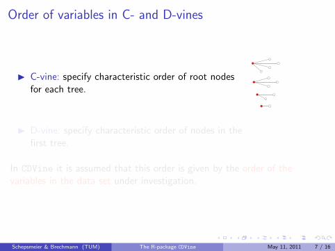
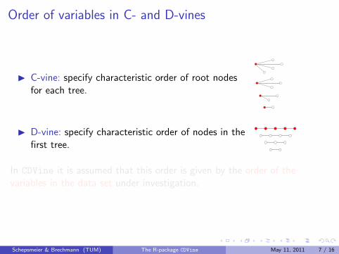
Order of variables in C- and D-vines
I C-vine: specify characteristic order of root nodesfor each tree.
1
1
1
1
1
1
1
1
1
1
I D-vine: specify characteristic order of nodes in thefirst tree.
In CDVine it is assumed that this order is given by the order of thevariables in the data set under investigation.
Schepsmeier & Brechmann (TUM) The R-package CDVine May 11, 2011 7 / 16
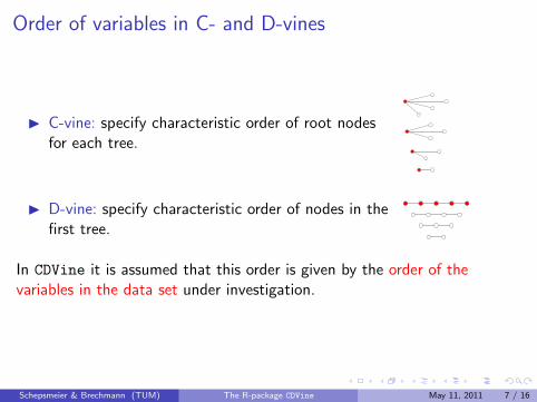
Order of variables in C- and D-vines
I C-vine: specify characteristic order of root nodesfor each tree.
1
1
1
1
1
1
1
1
1
1
I D-vine: specify characteristic order of nodes in thefirst tree.
1 1 1 1 1
1 1 1 1
1 1 1
1 1
In CDVine it is assumed that this order is given by the order of thevariables in the data set under investigation.
Schepsmeier & Brechmann (TUM) The R-package CDVine May 11, 2011 7 / 16
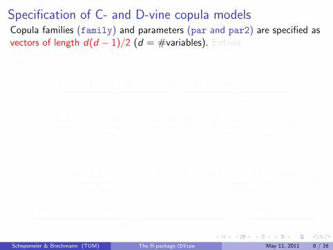
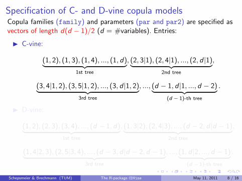
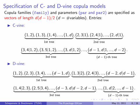
Specification of C- and D-vine copula modelsCopula families (family) and parameters (par and par2) are specified asvectors of length d(d − 1)/2 (d = #variables). Entries:
I C-vine:
(1, 2), (1, 3), (1, 4), ..., (1, d)︸ ︷︷ ︸1st tree
, (2, 3|1), (2, 4|1), ..., (2, d |1)︸ ︷︷ ︸2nd tree
,
(3, 4|1, 2), (3, 5|1, 2), ..., (3, d |1, 2)︸ ︷︷ ︸3rd tree
, ..., (d − 1, d |1, ..., d − 2)︸ ︷︷ ︸(d − 1)-th tree
.
I D-vine:
(1, 2), (2, 3), (3, 4), ..., (d − 1, d)︸ ︷︷ ︸1st tree
, (1, 3|2), (2, 4|3), ..., (d − 2, d |d − 1)︸ ︷︷ ︸2nd tree
,
(1, 4|2, 3), (2, 5|3, 4), ..., (d − 3, d |d − 2, d − 1)︸ ︷︷ ︸3rd tree
, ..., (1, d |2, ..., d − 1)︸ ︷︷ ︸(d − 1)-th tree
.
Schepsmeier & Brechmann (TUM) The R-package CDVine May 11, 2011 8 / 16
Example
Transformed residuals of daily log returns of major world stock indices in2009 and 2010 (396 observations):
S&P 500
Nikkei 225
SSE Composite Index
DAX
CAC 40
FTSE 100 Index
Load into workspace:
> data(worldindices)
Schepsmeier & Brechmann (TUM) The R-package CDVine May 11, 2011 9 / 16
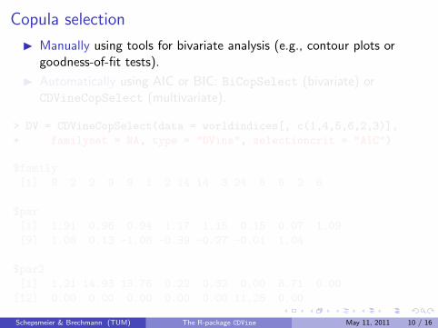
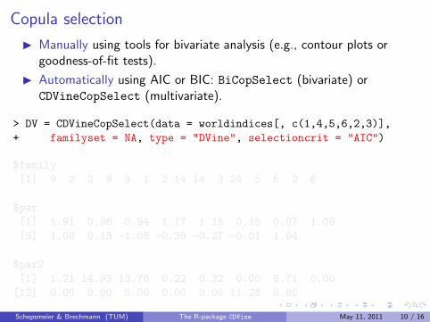
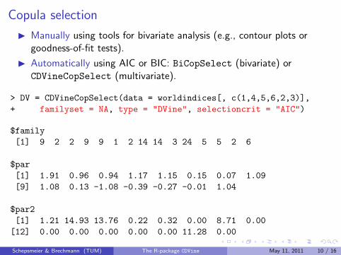
Copula selection
I Manually using tools for bivariate analysis (e.g., contour plots orgoodness-of-fit tests).
I Automatically using AIC or BIC: BiCopSelect (bivariate) orCDVineCopSelect (multivariate).
> DV = CDVineCopSelect(data = worldindices[, c(1,4,5,6,2,3)],
+ familyset = NA, type = "DVine", selectioncrit = "AIC")
$family
[1] 9 2 2 9 9 1 2 14 14 3 24 5 5 2 6
$par
[1] 1.91 0.96 0.94 1.17 1.15 0.15 0.07 1.09
[9] 1.08 0.13 -1.08 -0.39 -0.27 -0.01 1.04
$par2
[1] 1.21 14.93 13.76 0.22 0.32 0.00 8.71 0.00
[12] 0.00 0.00 0.00 0.00 0.00 11.28 0.00
Schepsmeier & Brechmann (TUM) The R-package CDVine May 11, 2011 10 / 16
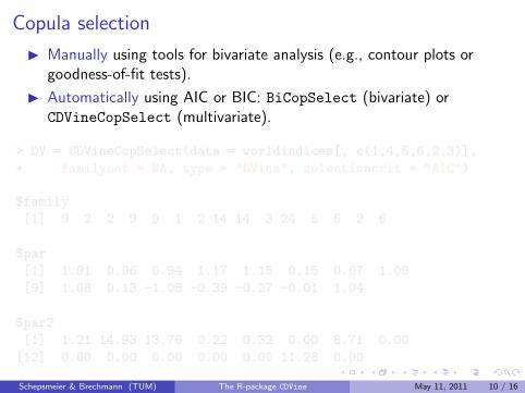
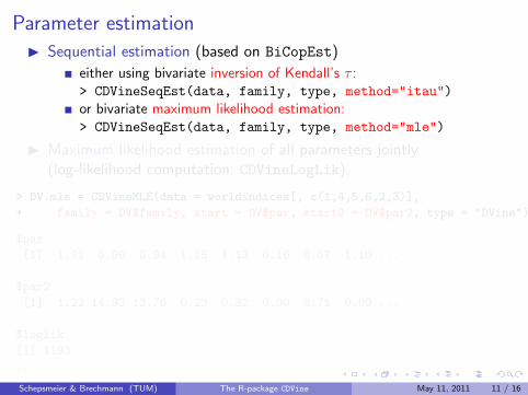
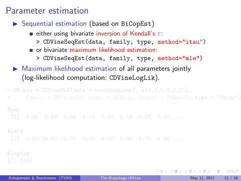
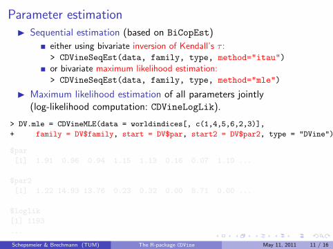
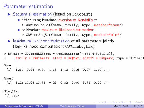
Parameter estimation
I Sequential estimation (based on BiCopEst)
either using bivariate inversion of Kendall’s τ :> CDVineSeqEst(data, family, type, method="itau")
or bivariate maximum likelihood estimation:> CDVineSeqEst(data, family, type, method="mle")
I Maximum likelihood estimation of all parameters jointly(log-likelihood computation: CDVineLogLik).
> DV.mle = CDVineMLE(data = worldindices[, c(1,4,5,6,2,3)],
+ family = DV$family, start = DV$par, start2 = DV$par2, type = "DVine")
$par
[1] 1.91 0.96 0.94 1.15 1.13 0.16 0.07 1.10 ...
$par2
[1] 1.22 14.93 13.76 0.23 0.32 0.00 8.71 0.00 ...
$loglik
[1] 1193
...
Schepsmeier & Brechmann (TUM) The R-package CDVine May 11, 2011 11 / 16
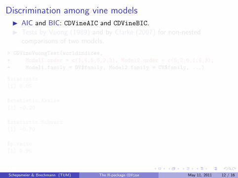
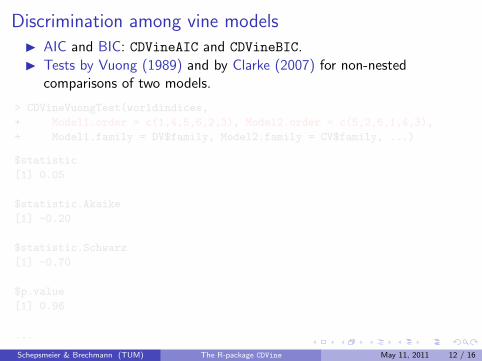
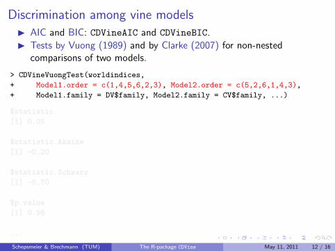
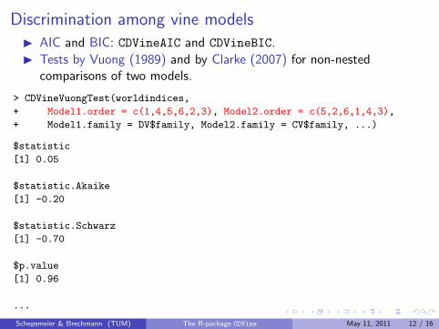
Discrimination among vine models
I AIC and BIC: CDVineAIC and CDVineBIC.
I Tests by Vuong (1989) and by Clarke (2007) for non-nestedcomparisons of two models.
> CDVineVuongTest(worldindices,
+ Model1.order = c(1,4,5,6,2,3), Model2.order = c(5,2,6,1,4,3),
+ Model1.family = DV$family, Model2.family = CV$family, ...)
$statistic
[1] 0.05
$statistic.Akaike
[1] -0.20
$statistic.Schwarz
[1] -0.70
$p.value
[1] 0.96
...
Schepsmeier & Brechmann (TUM) The R-package CDVine May 11, 2011 12 / 16
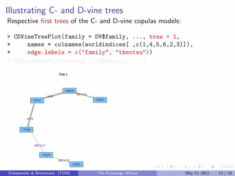
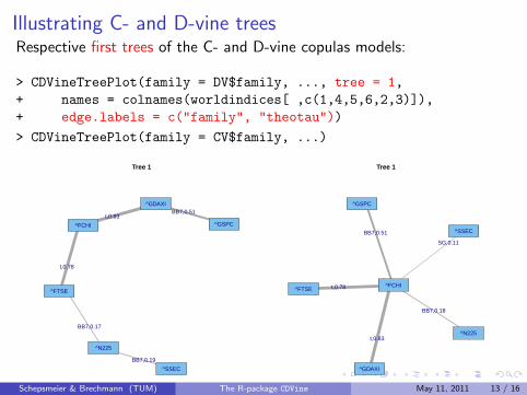
Illustrating C- and D-vine treesRespective first trees of the C- and D-vine copulas models:
> CDVineTreePlot(family = DV$family, ..., tree = 1,
+ names = colnames(worldindices[ ,c(1,4,5,6,2,3)]),
+ edge.labels = c("family", "theotau"))
> CDVineTreePlot(family = CV$family, ...)
Schepsmeier & Brechmann (TUM) The R-package CDVine May 11, 2011 13 / 16
Illustrating C- and D-vine treesRespective first trees of the C- and D-vine copulas models:
> CDVineTreePlot(family = DV$family, ..., tree = 1,
+ names = colnames(worldindices[ ,c(1,4,5,6,2,3)]),
+ edge.labels = c("family", "theotau"))
> CDVineTreePlot(family = CV$family, ...)
Tree 1
BB7,0.51t,0.83
t,0.78
BB7,0.17
BB7,0.19
^GSPC
^GDAXI
^FCHI
^FTSE
^N225
^SSEC
Tree 1
BB7,0.18
t,0.78
BB7,0.51
t,0.83
SG,0.11
^FCHI
^N225
^FTSE
^GSPC
^GDAXI
^SSEC
Schepsmeier & Brechmann (TUM) The R-package CDVine May 11, 2011 13 / 16
Summary & conclusion
Strong (positive) dependence among European indices.
European indices central to explaining overall dependence.
Indication of medium to strong tail dependence.
Asymmetric (conditional) dependencies.
No significant difference between C- and D-vine copula models.→ Different interpretations possible based on tree structures.
Schepsmeier & Brechmann (TUM) The R-package CDVine May 11, 2011 14 / 16
Bibliography
Aas, K., C. Czado, A. Frigessi, and H. Bakken (2009).Pair-copula constructions of multiple dependence.Insurance: Mathematics and Economics 44(2), 182–198.
Clarke, K. A. (2007).A simple distribution-free test for nonnested model selection.Political Analysis 15(3), 347–363.
Czado, C., U. Schepsmeier, and A. Min (2011).Maximum likelihood estimation of mixed C-vines with application to exchange
rates.To appear in Statistical Modelling .
Vuong, Q. H. (1989).Ratio tests for model selection and non-nested hypotheses.Econometrica 57(2), 307–333.
Schepsmeier & Brechmann (TUM) The R-package CDVine May 11, 2011 15 / 16

Thank you very much for your attention!
Visit: http://cran.r-project.org/web/packages/CDVine/
Schepsmeier & Brechmann (TUM) The R-package CDVine May 11, 2011 16 / 16