CDS and Equity Market Reactions to Stock Issuances in … · CDS and Equity Market Reactions to...

This paper presents preliminary findings and is being distributed to economists

and other interested readers solely to stimulate discussion and elicit comments.

The views expressed in this paper are those of the authors and do not necessarily

reflect the position of the Federal Reserve Bank of New York or the Federal

Reserve System. Any errors or omissions are the responsibility of the authors.

Federal Reserve Bank of New York

Staff Reports

CDS and Equity Market Reactions to Stock

Issuances in the U.S. Financial Industry:

Evidence from the 2002-13 Period

Marcia Millon Cornett

Hamid Mehran

Kevin Pan

Minh Phan

Chenyang Wei

Staff Report No. 697

November 2014

Revised December 2014

CDS and Equity Market Reactions to Stock Issuances in the U.S. Financial Industry:

Evidence from the 2002-13 Period Marcia Millon Cornett, Hamid Mehran, Kevin Pan, Minh Phan, and Chenyang Wei

Federal Reserve Bank of New York Staff Reports, no. 697

November 2014; revised December 2014

JEL classification: G01, G21, G32

Abstract

We study seasoned equity issuances by financial and nonfinancial companies between 2002 and

2013. To assess the risk and valuation implications of these issuances, we conduct an event-study

analysis using daily credit default swap (CDS) and stock market pricing data. The major findings

of the paper are that equity prices do not react to new issues in the pre-crisis period, but react

negatively in the crisis. CDS prices respond to new, default-relevant information. Over the full

sample period, cumulative abnormal CDS spreads drop in response to equity issuance

announcements. The reactions are significantly stronger during the financial crisis when the

federal government injected equity into financial institutions to ensure their viability. The market

reacted to this by assessing significantly lower costs for default protection via credit default

swaps on equity issue announcements. The evidence indicates that single-name CDS based on

financial firms’ default probabilities are potentially useful for private investors and regulators.

Key words: financial institutions, stock issuance, credit default swaps, financial crisis

_________________

Cornett: Bentley University (e-mail: [email protected]). Mehran: Federal Reserve Bank of

New York (e-mail: [email protected]). Pan: Harvard University (e-mail:

[email protected]). Phan: Federal Reserve Bank of New York (e-mail:

[email protected]). Wei: American International Group (e-mail: [email protected]).

The authors are grateful to Viral Acharya, Malcolm Baker, Patrick Bolton, Atul Gupta, Otgo

Erhemjamts, Mark Flannery, Charles Kahn, Jim Musumeci, Stewart Myers, Anjan Thakor, and

seminar participants at Bentley University for their helpful comments. The views expressed in

this paper are those of the authors and do not necessarily reflect the position of the Federal

Reserve Bank of New York or the Federal Reserve System.

1

CDS and Equity Market Reactions to Stock Issuances in the

U.S. Financial Industry: Evidence from the 2002 – 2013 Period

1. Introduction

Financial theory and empirical analysis has shown that, because security values are

determined by the distribution of the market value of a firm’s assets, market prices of different

securities issued by a firm are closely linked. Specifically, market prices of financial securities

issued by firms should reflect the default risk of the firms. Less explored is the relation between

market prices of various credit related securities for the same firm. For example, the link between

the relatively new, but fast growing credit derivatives market and equity markets has only begun to

be explored.1 One such market is the single name credit default swap (CDS) market. A single

name CDS is a contract that provides protection against a default event involving a single issuer,

or ‘name.’ Therefore, single name CDS contracts should reflect the pure issuer default risk of a

firm irrespective of any issue specific risk. Thus, single name CDS contracts are of particular

interest in that they may serve as a benchmark for measuring and pricing credit risk of a firm.

CDS prices arguably are related to the health of financial institutions. Banks are required to

maintain adequate capital due to regulatory requirements. While the market and regulators may

have assessed that banks were adequately capitalized prior to 2008, the perception changed with

the failure of Bear Stearns. In addition to TARP capital infusions during the crisis, banks in effect

were forced to issue large amounts of equity capital (and forgo payouts) to manage their risk, thus

establishing a viable business model (and also to payback the TARP funds). As a result, the

reaction of CDS prices to equity issuances may be different before versus during the crisis. The

effect of equity issuances in turn may be related to whether or not banks could use the proceeds for

1 For example, Norden and Weber (2009) analyze the relationship between credit default swap (CDS), bond, and stock

markets between 2000 and 2002. Focusing on the intertemporal co-movement, they find that stock returns lead CDS

and bond spread changes. Further, they find that the CDS market is more sensitive to the stock market than the bond

market and the strength of the co-movement increases the lower the credit quality and the larger the bond issues.

2

asset funding and/or maintaining their capital needs. Practitioners recognize that while equity

issuances can help with asset funding, the issues typically are much more important for solvency

(which supports asset funding on a larger scale).2 Figure 1 shows the shows the empirical

distribution of the Tier 1 capital gap for 39 bank equity issuances during the sample period. The

Tier 1 gap is calculated as the difference between the financial firm’s Tier 1 risk-based capital

ratio the quarter before the equity issue announcement and the FDIC benchmark of 6% required to

be classified as a well-capitalized institution.3 A negative Tier 1 gap means that the institution’s

Tier 1 capital ratio falls below that threshold. In the quarter before announcing an equity issuance,

21 of the 39 banks have a Tier 1 capital ratio below 6%. Thus, it is always true that equity

issuances directly help reduce funding pressure by the amount raised, and often true that they help

improve funding capability indirectly by improving solvency.

In this paper, we study equity and CDS market reactions to 129 seasoned equity issuances

that were announced by 56 financial companies between 2002 and 2013. For a baseline

comparison, we examine similar announcement returns for 356 issues by 172 nonfinancial firms

over the same period. We do this as the purpose behind equity issuance by financials may be

different than nonfinancials; for example, as stated earlier, to address capital requirements as

opposed to funding needs. The perception of capital needs changed over the sample period due to

adoption of new capital requirement(s) and market assessment of implication no bailout policy

2 Mehran and Thakor (2011) address the question of whether there is an optimal capital structure for each bank, and if

so, what this implies about how bank capital and value are related in the cross-section within the context of bank

mergers and acquisitions. The main result of their model is that there is an optimal capital structure for each bank, and

in the cross-section of banks, value is increasing in capital. This is counter to what is popularly believed: that bank

value is decreasing in capital. In fact, bank capital positively affects total bank value. The results are both statistically

and economically significant. Proposition 1 establishes that banks that keep higher equity capital monitor more. The

intuition is clear: a bank that keeps more equity faces a lower probability of being closed and hence a higher

probability of retaining its relationship banking rents, which are increasing in monitoring. Proposition 2 shows that

while the marginal benefit of equity identified in Proposition 1 is the same for all banks, the marginal cost of equity is

not, so equity is less attractive to banks with higher marginal cost of equity. This finding has the important implication

that banks choose to keep capital voluntarily (i.e., in the absence of capital requirements). 3 See https://www.fdic.gov/regulations/laws/rules/2000-4500.html.

3

regime under Dodd-Frank legislation. As a result, financial firms raised fresh capital through new

equity issuances. To better understand the purpose behind the issuances, we split the sample

period, analyzing market reactions before versus during the financial crisis. We take a unique

approach to measuring a change in the market’s perception of the probability of firm default. We

collect and analyze CDS data to assess the risk and valuation implications of these seasoned equity

issuances. We focus on financial institutions because they were heavily involved in, and some

would argue at the center of, the financial crisis. Further, unlike any other industry, financial

institutions were required to increase capital during and after the crisis. Thus, this industry

represents a unique opportunity to examine the relation between single name CDS securities and

equity securities issued by the firms.

Consistent with previous empirical findings, we find that the stock market generally reacts

negatively to announcements of common stock issuances by financial firms: the three-day

cumulative abnormal stock returns (CARs) average -1.43% percent over the sample period. We

also find that reactions are more negative during the financial crisis, albeit not significantly so: the

average CARs range from -1.58% to -2.02% during the sample period (although announcement

returns are insignificant in the pre-crisis period). Stock market reactions to equity issuances by

nonfinancials have a similar pattern to that reported in earlier research, i.e., negative and

significant throughout the sample period (the overall reaction is a loss of 2.87%). The pre-crisis

CARs for nonfinancial firms with single name CDS securities traded is in the order 1.10% to

1.77%, while crisis period CAR is about 3.8%. Nonfinancial equity issuers face larger losses

during crisis than financials.

We also find that CDS prices respond quickly to new default-relevant information. Over

the full sample period, cumulative abnormal CDS spreads (CAS) drop significantly (by an average

4

of 10.12 bps) in response to equity issuance announcements by financial firms. However, the

results are due to crisis period events only. The mean CASs is significant in the crisis period

(ranging from -16.15 bps to -18.84 bps), but is insignificant for pre-crisis events. These patterns

are not found for nonfinancial firms that issue equity over the same period, the overall effect is

insignificant (although CAS is negative and significant (ranging from -3.26 to -4.80 bps) in the

pre-crisis period). Cross-sectional analysis suggests that riskiness of the institution is one of the

key determinants of both abnormal stock returns and abnormal CDS spreads. Equity issuances by

riskier institutions (rated speculative grade) are received more favorably in the CDS market and by

stock investors. However, the relations fail to hold during the financial crisis.

During the financial crisis, the federal government injected equity (through the TARP

program) into financial institutions. The equity was made senior to common stock, but not to other

capital providers. Thus, the market reacted to this by assessing lower costs for default protection

via credit default swaps and insignificant changes in returns on equity issue announcements.

Further, creditors obtained an additional buffer against losses in the event of default. As a result,

the certification effect of an equity issue announcement prior to the financial crisis was not

necessarily the dominant effect during the crisis. During the financial crisis, issuances of equity by

higher risk financial firms did not provide the same degree of default-relevant information as they

did before the crisis. Thus, the evidence indicates that single named CDSs based on financial

firms’ default probabilities are potentially useful for private investors and regulators.

The remainder of the paper is organized as follows. Section 2 summarizes recent research

on CDS contracts as measures of default risk. Section 3 describes the data and methodology used

in the analysis. Section 4 discusses the results. Finally, Section 5 concludes the paper.

5

2. CDS contracts as a measure of default risk

In this paper, we take a unique approach to measuring a change in the market’s perception

of the probability of a debt default. Specifically, we collect and analyze single name credit default

swap data. In the event of a default, the CDS writer compensates the CDS buyer for losses on a

given face value of the underlying debt. The spread on the CDS contract is the price paid to the

writer of the CDS for selling this insurance contract to the CDS buyer. When the market perceives

that the probability of a debt default decreases (increases), the spread charged on the CDS

decreases (increases). Thus, we use changes in the CDS spread to measure changes in the market’s

perception of the probability of a debt default.

Several papers have examined the ability of CDS spreads to measure risk. Hull et al.

(2004) explore the extent to which credit rating announcements by Moody’s are anticipated by

participants in the credit default swap market. They conclude that either credit spread changes or

credit spread levels provide helpful information in estimating the probability of negative credit

rating changes. Jorion and Zhang (2007) examine the intra-industry information transfer effect of

Chapter 11 bankruptcies, Chapter 7 bankruptcies, and jump events, as captured in the credit

default swaps (CDS) and stock markets. They find strong evidence of contagion effects (positive

correlations across CDS spreads) for Chapter 11 bankruptcies and competition effects (negative

correlations across CDS spreads) for Chapter 7 bankruptcies. They also find that a large

unanticipated jump in a company’s CDS spread leads to the strongest evidence of credit contagion

across the industry. Ismailescu and Kazemi (2010) examine the effect of sovereign credit rating

change announcements on the CDS spreads of the event countries, and their spillover effects on

other emerging economies’ CDS premiums. They find that positive events have a greater impact

on CDS markets in the two-day period surrounding the event, and are more likely to spill over to

6

other emerging countries. Alternatively, CDS markets anticipate negative events, and previous

changes in CDS premiums can be used to estimate the probability of a negative credit event.

Most recently, papers have focused on CDS spread movements around the financial crises

in the U.S. and Europe. For example, Fontana and Scheicher (2010) study the relative pricing of

euro area sovereign CDS and the underlying government bonds for ten euro area countries from

January 2006 to June 2010. They find that, since September 2008, CDS spreads have on average

exceeded bond spreads, which may have been due to ‘flight to liquidity’ effects and limits to

arbitrage. Arce et al. (2012) analyze the extent to which prices in the sovereign CDS and bond

markets reflect the same information on credit risk in the context of the European Monetary

Union. They find that there are persistent deviations between both spreads during the crisis. Levels

of counterparty and global risk, funding costs, market liquidity, volume of debt purchases by the

European Central Bank in the secondary market, and the banks’ willingness to accept losses on

their holdings of Greek bonds are found to be significant factors in determining which market

leads price discovery. Andenmatten and Brill (2011) test whether the co-movement of sovereign

debt CDS premia increased significantly after the Greek debt crisis started in October 2009. Their

results indicate that during the Greek debt crisis there were not only periods of interdependence,

but also periods characterized by a significant increase in the co-movement of sovereign credit risk

as measured in CDS premia.

Di Cesare and Guazzarotti (2010) examine the determinants of credit default swap spread

changes for a large sample of U.S. nonfinancial companies from January 2002 and March 2009.

They use variables that have previously been found to have an impact on CDS spreads. Since the

onset of the crisis, they find that CDS spreads have become much more sensitive to the level of

leverage, while volatility has lost its importance. They also show that since the beginning of the

7

crisis CDS spread changes have been increasingly driven by a common factor, which cannot be

explained by indicators of economic activity, uncertainty, and risk aversion. Alexopoulou et al.

(2009) confirm the existence of a long-run relationship between CDS and corporate bond markets,

and the tendency for CDS markets to lead corporate bond markets in terms of price discovery.

They find that the outbreak of the financial crisis induced a substantial increase in risk aversion

and a shift in the pricing of credit risk, with CDS markets becoming more sensitive to systematic

risk, while bond markets priced in more information about liquidity and idiosyncratic risk.

Moreover, the crisis also brought about a systematic disconnection between the two markets

caused by the significant change in the lead-lag relationship, with CDS markets always leading

bond markets. Finally, Galil et al. (2014) use a cross-sectional analysis to investigate the

determinants of CDS spreads around the financial crisis. Fundamental variables such as historical

stock returns, historical stock volatility, and leverage explain CDS spreads after controlling for

ratings. During the crisis, while fundamental variables maintained their explanatory power, the

explanatory power of ratings decreased to almost zero.

A few recent studies have focused on single name CDS spreads for financial firms. For

example, Kallestrup et al. (2012) show that financial linkages across borders are priced in the CDS

markets beyond what can be explained by exposure to common factors. They construct a measure

which takes into account the relative size and riskiness of bank exposures to domestic government

bonds and other domestic residents. This measure helps explain the dynamics of bank CDS premia

after controlling for country specific and global risk factors. Demirguc-Kunt et al. (2010)

investigate the impact of government indebtedness and deficits on bank stock prices and CDS

spreads for a sample of international banks. They find that the change in bank CDS spreads in

2008 relative to 2007 reflects countries’ deterioration of public deficits. Ballester et al. (2013) use

8

bank CDS spreads to evaluate contagion among banks and banking sectors in different countries

during the financial crisis. They find the Eurozone troubles barely affected U.S. banks. De

Bruyckere et al. (2013) use correlations in CDS spreads at the bank and at the sovereign level to

document significant contagion between bank and sovereign credit risk during the European

sovereign debt crisis.4 Possibly most relevant for our study, Flannery et al. (2010) evaluate the

viability of credit default swaps (CDS) spreads as substitutes for credit ratings for large financial

institutions that were prominently involved in the financial crisis. They show that CDS spreads

incorporate new information about as quickly as equity prices and significantly more quickly than

credit ratings.

3. Data and methodology

3.a. Data

The initial sample examined in this paper includes all U.S. financial institutions that issued

equity between 2002 and 2013.5 This sample is collected from S&P’s Capital IQ database. We

then limit the sample to those financial firms having CDS pricing data reported by Markit.6 The

final sample we examine includes data on 129 equity issuances by 56 financial institutions.7 Table

1 lists some descriptive statistics of the sample by-year: including the number of announcements,

the total amount of equity issued, and the means and standard deviations of the distributions of

4 Eichengreen et al. (2009) identify common factors in the movement of banks' credit default swap spreads. They find

that fortunes of international banks rise and fall together even in normal times along with short-term global economic

prospects. But the importance of common factors rose to exceptional levels from the outbreak of the financial crisis to

past the rescue of Bear Stearns, reflecting a diffuse sense that funding and credit risk was increasing. Following the

failure of Lehman Brothers, the interdependencies briefly increased to a new high, before they fell back to the pre-

Lehman elevated levels. 5 The sample firms include all U.S. financial companies except for REITs, due to their distinct organizational

structure. 6 Markit is a private company headquartered in London. The firm provides CDS end-of-day quotes for approximately

450 of the most liquid CDS contracts, including G20 sovereigns and large financial corporations. 7 Issuance transactions with public offering or shelf registration features are excluded as are non-secondary issue

related transactions.

9

relative size of the equity issuances. The table shows a fairly balanced flow in financial

institutions’ equity issuance activities between the first and the second half of the sample period,

with the largest frequency of issues coming in 2008 and 2009. These two years also see the largest

issue amounts, $90.68 billion in 2008 and $72.08 billion in 2009. The vast majority of these

issuances are from financial firms. Indeed, panel B of table 1 reports the mean relative issue size

(dollar value of equity issuance relative to market capital) for financial firms is 24.36% in 2008

and 8.67% for nonfinancial firms: the difference is significant at better than 1%. Financial firms

issue significantly more relative equity than nonfinancial firms in every year during the crisis

period except 2012. The Figures 1 and 2 illustrate the general movements of the CDS spreads and

stock market values during the sample period. Figure 2 plots a daily series of the mean CDS

spreads of our sample firms and Figure 3 plots the daily evolution of the combined equity market

capitalization8 of the sample firms. Note the significant increase in CDS spreads and decrease in

financial firm values during the financial crisis.

We examine stock returns and CDS spreads for the whole sample period, as well as two

sub-periods, termed in the paper, the “pre-crisis” and the “crisis” periods. We experiment with two

cutoff dates to delineate the pre-crisis and crisis periods using two prominent events in 2008:

3/24/2008 (the collapse of Bear Stearns) and 10/14/2008 (the TARP Capital Purchase Program

announcement). Signs of significant problems in the U.S. economy first arose in late 2006 and the

first half of 2007 when home prices plummeted and defaults by subprime mortgage borrowers

began to affect the mortgage lending industry as a whole, as well as other parts of the economy

noticeably. As mortgage borrowers defaulted on their mortgages, financial institutions that held

these mortgages and mortgage backed securities started announcing huge losses on them. A prime

8 Equity market capitalization is calculated as the daily stock price times the number of shares of common stock

outstanding (from CRSP data tapes).

10

example of the losses incurred is that of Bear Stearns. In the summer of 2007, two Bear Stearns

hedge funds suffered heavy losses on investments in the subprime mortgage market. The two

funds filed for bankruptcy in the fall of 2007. Bear Stearns’ market value was hurt badly from

these losses. The losses became so great that in March 2008 J.P. Morgan Chase and the Federal

Reserve stepped in to rescue the then fifth largest investment bank in the United States before it

failed or was sold piecemeal to various financial institutions. On March 24, 2008, J.P. Morgan and

Bear Stearns announced a merger agreement. J.P. Morgan Chase purchased Bear Stearns for $236

million, or $2 per share. The stock was selling for $30 per share three days prior to the purchase

and $170 less than a year earlier. The collapse of Bear Stearns and its sale to J.P. Morgan marked

the beginning of the mortgage crisis for major financial institutions.9

On October 14, 2008, then-Secretary of the Treasury Paulson announced a revision in

TARP implementation in which the Treasury directly injected up to $250 billion10

of TARP funds

(through the Capital Purchase Program (CPP)) into the U.S. banking system through the purchase

of senior preferred stock and warrants in qualifying financial institutions (QFIs).11

The CPP was

intended to inject equity into financial institutions that were suffering from temporary liquidity

and other financial problems due to the financial crisis, but were otherwise in decent shape. By the

time it closed on December 31, 2009, 707 applications were approved and funded by the Treasury

through the CPP.12

9 Using principal components analysis to identify common factors in the movement of banks' credit default swap

spreads, Eichengreen et al. (2012) find that the importance of common factors rose steadily to exceptional levels from

the outbreak of the Subprime Crisis to past the rescue of Bear Stearns, reflecting a diffuse sense that funding and

credit risk was increasing. 10

This amount was eventually lowered to $204.9 billion. 11

Qualifying financial institutions (QFIs) include bank holding companies, financial holding companies, insured

depository institutions, and savings and loan holding companies that are established and operating in the United States

and that are not controlled by a foreign bank or company. 12

Cornett et al. (2013) look at how the pre-crisis health of banks is related to the probability of receiving and repaying

TARP capital. They find that financial performance characteristics that are related to the probability of receiving

TARP funds differ for the healthiest (“over-achiever”) versus the least healthy (“under-achiever”) banks. Ng et al.

11

3.b. Seasoned equity issues of nonfinancial firms

In order to examine whether any observed relation between CDS spreads and equity

market reactions is unique to financial firms, we also collect information on equity issuances by

nonfinancial firms between 2002 and 2013. The initial sample of nonfinancial firm equity

issuances is also collected from S&P’s Capital IQ database. We then limit the sample to those

nonfinancial firms having CDS pricing data reported by Markit. The final sample of nonfinancial

firms we examine includes data on 356 equity issuances by 172 firms. Table 1 lists the year-by-

year distribution of the announcements.

3.c. Calculation of cumulative abnormal stock returns (CARs)

We use standard event study techniques to calculate unexpected changes in stock prices in

response to equity issue announcements by the sample firms. Stock return data are collected from

the Center for Research in Security Prices (CRSP) data tapes. Stock return data are identified for

54 of the 56 financial firms (123 of the 129 equity issue announcements) and 170 of the 172

nonfinancial firms (337 of the 356 events). We calculate normal stock return performance using a

125 trading day window, ending five trading days before the announcement date. A Fama-French

three factor model is used to predict the expected excess return:13

Returnexcess i,t = α + β1(Market – Rf)t + β2(SMB)t + β3(HML)t (1)

where Rf is the risk-free return rate, SMB stands for "small (market capitalization) minus big," and

HML stands for "high (book-to-market ratio) minus low."

(2011) find that publicly traded TARP banks experienced significantly lower equity returns relative to non-TARP

banks during TARP’s initiation period. They also find that equity markets adjusted the values of the TARP banks

upward in the quarters following TARP injections. Veronesi and Zingales (2010) also provide an analysis of the

valuation effects of TARP, but for just the initial financial institutions that received TARP infusions on October 14,

2008. They find that, while the primary effect of TARP was to benefit bondholders, the program created little value

for shareholders. While they find that valuation benefits for banks exceeded the costs imposed on taxpayers, they

argue that other potential rescue strategies would have yielded larger net benefits. 13

We also examined a specification where excess return is a function of the three Fama-French factors and an

additional momentum factor. Results are similar to those reported in tables 3, 5, and 6. They are available from the

authors on request.

12

The abnormal return, ARi,t, is then calculated as the actual, Returnexcess, less the predicted,

Returnexcess. Summation over the three-day window (the trading day before the announcement, the

announcement day, and the following trading day) gives the three-day announcement period

cumulative abnormal stock returns (CARs):

CAR (-1,1)i = ARi,-1 + ARi,0 + ARi,1 (2)

3.d. Calculation of cumulative abnormal CDS spread (CAS)

We also use standard event study techniques to calculate unexpected changes in CDS

spreads in response to the announcement events. First, we calculate daily CDS abnormal spreads

(AS) for each contract as:

ASi,t = Spreadi,t − Rating_Matched_Index_Spreadt (3)

where Spreadi,t is the end-of-day spread quote of contract i on event day t, and is the rating-

matched (investment-grade or speculative-grade) CDS index spread on event day t. We then

calculate the three-day cumulative CDS abnormal spread (CAS) for each contract as:

CASi,t = ASi,1 −ASi,-1 (4)

where ASi,1 is the CDS abnormal spread at the end of the next trading day after the equity issuance

announcement by firm i, and ASi,−1 is the CDS abnormal spread one day before the announcement.

Unexpected movements in the CDS spread measure the perceived impact on the cost of

purchasing default insurance on the issuing institution. Unexpected changes in stock returns

measure the valuation impact on the residual claimholders (shareholders) due to the firm’s equity-

raising action. Throughout the analysis, we use the three-day cumulative abnormal CDS spread

(CAS) and cumulative abnormal stock return (CAR) as the key measures of the market reactions.

4. Results and discussions

13

4.a. Average unexpected reactions in CDS and equity markets

Table 2 summarizes CDS market reactions to 129 seasoned equity issuance announcements

made by 56 financial firms and 356 announcements made by 172 nonfinancial firms between 2002

and 2013. We report the average CAS for the whole sample period and two sub periods, the “pre-

crisis” period and “crisis” period. Panel A presents results based on the split using the collapse of

Bear Stearns (3/24/2008) to delineate the beginning of the crisis period and panel B reports

numbers based on the split using the TARP CPP announcement (10/14/2008) to delineate the

beginning of the crisis period.

Over the entire sample period, 2002 through 2013, the market-adjusted CDS spread for

financial firms (i.e., the default insurance premium) drops by an average 10.12 bps (see row

“Total”) over a three-day window in response to equity issuances announcements. This effect is

statistically significant at the 1% level, suggesting that equity financing activities by financial

firms are generally favorably received by CDS investors. That is, the price of default insurance, in

the form of CDS, decreases at the announcement of stock issuances by financial firms.

Looking at results for the two sub-periods, we see that significantly stronger reactions are

concentrated in the crisis period. Using the acquisition of Bear Stearns by J.P. Morgan to delineate

the start of the crisis, the three-day average CAS is -16.15 bps in the crisis period (panel A). Using

the announcement of the TARP CPP program to delineate the start of the crisis, the two-day

average CAS is -18.84 bps in the crisis period (panel B). In contrast, pre-crisis period estimated

reactions appear to be insignificant both statistically and economically. Using the acquisition of

Bear Stearns by J.P. Morgan to delineate the start of the crisis, the average CAS is -2.75 bps in the

pre-crisis period (panel A). Using the announcement of the TARP CPP program to delineate the

start of the crisis, the average CAS is -2.54 bps in the pre-crisis period (panel B). In both cases, the

14

crisis period CAS estimates are highly significant and larger in magnitude than the pre-crisis

period (the t-statistics for the differences in CAS between the crisis and pre-crisis period are 1.93

(significant at 5.7%) and 2.07 (significant at 4.2%) in panels A and B, respectively.

The estimated reactions appear economically significant when benchmarked with the

normal market level in the 2002-2008 period. The raw CDS spread of the sample firms averages

around 70 bps in this period. With this backdrop, the market-adjusted reaction in the crisis period

accounts for more than 20% (e.g., -16.15 bps/70 bps) of the general market level in the pre-crisis

period, regardless of the cutoff point we use for defining the crisis period. Thus, equity financing

activities by financial firms are received most favorably by CDS investors in the crisis period.

Financial firms that issued stock during the financial crisis experienced a steep drop in the price of

default insurance.

Finally, comparing the results for financial firms to those of nonfinancial firms, we find

differences. Using the acquisition of Bear Stearns by J.P. Morgan to delineate the start of the crisis

period, the two-day average CAS for nonfinancial firms is -42.71 bps in the crisis period (panel

A). Using the announcement of the TARP CPP program to delineate the start of the crisis period,

the two-day average CAS is -45.70 bps in the crisis period (panel B). In contrast to the results for

financial firms, neither of these is statistically significant. However, estimated reactions in the pre-

crisis period appear to be significant. The two-day average CAS is -3.26 bps (significant at 10%)

in panel A and -4.80 bps (significant at 5%) in panel B. Finally and in contrast to the results for

financial firms, for nonfinancial firms the crisis period CAS estimates are not significantly

different from the pre-crisis period CAS estimates (the t-statistics for the differences in CAS

between the crisis and pre-crisis period are 1.32 and 1.24 in panels A and B, respectively).

15

Table 3 presents evidence on the stock market reactions to stock issue announcements by

financial and nonfinancial firms. Adjusted for systematic pricing factors, the stock market overall

reacted negatively to seasoned stock offerings by financial firms over the period 2002 through

2013.14

Three-day cumulative abnormal stock returns (CARs) average -1.43%, significant at the

10% level. This magnitude is comparable with earlier evidence, e.g., Cornett et al. (1998) find an

average two-day CAR of -1.62% for seasoned equity issuances by financial institutions.

Looking at the pre-crisis and the crisis periods separately, we find insignificantly larger

(negative) reactions in the crisis period. Using the acquisition of Bear Stearns by J.P. Morgan to

delineate the start of the crisis period, the mean CAR, -0.69%, is insignificant in the pre-crisis

period. However, common stock issuances induce an average CAR of -2.02% (significant at 10%)

in the crisis period. Using the announcement of the TARP CPP program to delineate the start of

the crisis period, the pre-crisis mean CAR is -1.30%, while the crisis period mean CAR is -1.58%

(both are insignificant). Further, the t-statistics for the differences in CAR between the crisis and

pre-crisis period are 0.85 in panel A and 0.18 in panel B and are both are insignificant.

While the general conclusion from these results are that financial firm stock return

reactions to seasoned equity issuances are not significantly different before versus during the

financial crisis, when benchmarked with normal market conditions, the estimated market reactions

appear rather significant. For example, during the crisis period, the average CAR (-2.02%, using

the acquisition of Bear Stearns by J.P. Morgan as the start of the crisis period) is almost 40 times

larger than the average raw return (0.051%) of the issuing institutions’ stocks in the pre-crisis

period. Thus, during the crisis, stock investors held markedly more negative views toward

financial firms’ equity financing activities.

14

We were only able to obtain stock market data for 123 of the 129 equity issue announcements by financial firms and

337 of the 356 announcements by nonfinancial firms. Thus, the number of events drops slightly.

16

As mentioned above, the TARP CPP was intended to inject equity into financial

institutions that were suffering from temporary liquidity and other financial problems due to the

financial crisis, but were otherwise in decent shape. These government capital injections need to

be analyzed not only in terms of certification effects, but also in terms of how they impact investor

perceptions of future regulatory action. While a capital injection certainly implies confidence in a

financial firm’s viability, it is different from a pure certification exercise like the Supervisory

Capital Assessment Program (SCAP, more often known as bank stress tests) or the Depression-era

bank holiday in that it alters the risk to taxpayers from a subsequent failure and may therefore

influence regulators' behavior. Before the crisis, the U.S. government typically stood in a ‘third-to-

default” position (through the FDIC guarantee on deposits) behind shareholders, other capital

providers, and unsecured creditors. After a TARP CPP injection, it moved to a “second-to-default”

position behind shareholders.

It is worth pausing to consider what counts as “default” in this context. Under the terms of

the FDICIA of 1991, banks are not subject to regular bankruptcy proceedings with normal creditor

rights (the Wall Street Reform and Consumer Protection Act of 2010 has effectively extended this

treatment to a range of financial holding companies). The event of default is the point at which the

FDIC seizes the operating bank subsidiary; the common equity of the bank is typically wiped out

entirely and unsecured creditors are provided with a discounted payoff decided by the FDIC. Well

ahead of seizure, however, the bank's supervisors might also force the bank to raise capital even if

this issuance is not in the best interest of shareholders.15

The analytical objective for an analyst or

investor is therefore to judge when regulatory intervention will occur and what losses they are

subjected to post-intervention.

15

One can imagine that investors, in an uncorrelated but otherwise identical set of banks, might decide to limit their

losses on any one bank in order to preserve their upside gains on the portfolio as a whole.

17

The immediate reaction to the announcement of capital injections through the TARP CPP

focused on the certification effect; the program targeted “healthy” banks, the terms of the

preferred stock seemed attractive, and the objective appeared to be to boost confidence in the

financial system. The fact that government capital was now subordinate to unsecured creditors

also served as a form of “seizure insurance” for anxious investors who had just experienced the

shock of government-imposed losses on the collapse of Washington Mutual. But what happened

next is instructive:

1. Bank capital has historically been measured mainly on the basis of Tier 1 capital ratios

((common equity + qualifying preferred stock) to risk-weighted assets). Differences in Tier

1 capital ratios across banks provided important information about banks' relative

profitability, risk tolerance, and access to capital. Analysts and money managers used Tier

1 capital ratios almost exclusively to identify differences among banks. Preferred stock

issued to the government through the TARP CPP qualified as Tier 1 capital. The injection

of government capital, which amounted to approximately 3% of risk-weighted assets for

virtually all publicly traded banks, made Tier 1 comparisons less meaningful.16

Not

surprisingly, the focus of analysts and money managers shifted to the Tangible Common

Equity (TCE) ratio (common equity to tangible assets) since this measure did not include

TARP CPP preferred stock: comparisons made on the basis of TCE remained undiluted.

By early 2009 market participants were focusing almost exclusively on TCE and Tier 1

Common (common equity to risk-weighted assets) ratios. In the process, TARP CPP

capital, as well as all other non-common equity Tier 1 capital, issued by banks had become

essentially moot as measure used to evaluate bank health.

16

Indeed, in a couple of cases that banks canceled planned equity raises once CPP was announced – a great real world

example of Gresham's law at work.

18

2. By design preferred stock issued through TARP CPP, was made senior to common equity

in order to protect taxpayers from loss. So, while creditors obtained an additional buffer

against losses in the event of default, shareholders did not – they remained in a first loss

position. Shareholders might reasonably suspect that the government would be more prone

to intervene if a TARP CPP bank got into trouble given that the government was now in a

second loss position and had lost the buffer provided by other forms of regulatory capital

and unsecured debt. Indeed, the higher loss outcomes could more than offset the

certification effect. However, the continued decline in bank stocks in the period between

the announcement of TARP CPP and the release of the first bank stress test (SCAP) results

(see Figure 3) suggests equity investors did not in fact see TARP CPP capital injections as

reducing their risk. Moreover, the unpopularity of the program, the addition of “strings” by

Congress and the focus on getting the money back all made TARP CPP increasingly seem

like expensive capital17

that could not absorb losses or be leveraged like common equity.

Given these two considerations, it is not surprising that equity market reactions to new stock

issuances by financial firm are larger in the crisis period relative to the pre-crisis period. However,

while equity market reactions are larger in the crisis period, they are not significantly so. In part,

this may be because the certification effect was more robust; differentiating amongst banks in

terms of capital needs provided more information and the capital raised was fully loss absorbing.18

17

As public outrage swelled over the rapidly growing cost of ‘bailing out’ financial institutions, the Obama

administration and lawmakers attached more and more restrictions on banks that received TARP funds. For example,

with the acceptance of TARP funds, banks were told to put off evictions and modify mortgages for distressed

homeowners, let shareholders vote on executive pay packages, slash dividends, and withdraw job offers to foreign

citizens. Some bankers stated that conditions of the TARP program had become so onerous that they wanted to return

the bailout money as soon as regulators set up a process to accept the repayments. For example, just three months after

receiving TARP funds, Signature Bank of New York announced that because of new executive pay restrictions

assessed as a part of the acceptance of TARP funds, it notified the Treasury that it intended to return the $120 million

it had received. 18

It is also instructive to contrast the reaction to TARP CPP with the subsequent release of stress test results and

associated capital raising. Even though many banks were forced to undertake dilutive capital raises to satisfy the

19

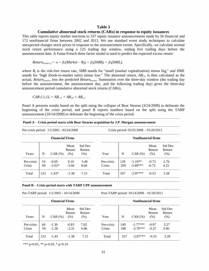
Finally from table 3, comparing the results for financial firms to those of nonfinancial

firms, we again find differences. Using the acquisition of Bear Stearns by J.P. Morgan to delineate

the start of the crisis period, the two-day average CAR for nonfinancial firms is -1.10% in the pre-

crisis period (panel A). Using the announcement of the TARP CPP program to delineate the start

of the crisis period, the two-day average CAR is -1.77% in the pre-crisis period (panel B). In

contrast to the results for financial firms, both of these are significant at 5% and 1%, respectively.

However, neither is significantly different from the CARs for financial firms (-0.69% and -1.30%,

respectively). Similarly, in the crisis period the two-day average CAR is -3.89% (significant at

1%) in panel A and -3.70% (significant at 1%) in panel B. In contrast to the results for financial

firms, the crisis period CARs are significantly larger than the pre-crisis period CARs (the t-

statistics for the differences in CARs between the crisis and pre-crisis period are 5.00 and 2.96 in

panels A and B, respectively). Finally, the crisis period CARs for nonfinancial firms are larger

than the crisis period CARs for financial firms (the t-statistics for the differences in CARs are 1.55

and 1.73 in panels A and B, respectively).

Remembering that the TARP CPP program injected capital into financial institutions that

were suffering from temporary problems, these results make sense. TARP CPP injections certified

the long-term viability of the financial firms that received funds. However, TARP CPP funds were

not provided to nonfinancial firms. As a result, these firms were left more susceptible to losses and

even failure resulting from the financial crisis. Thus, it is not surprising that the crisis period

CARs for financial firms (that were receiving capital injections from the federal government) are

SCAP requirements and/or exit TARP, share prices generally rallied. This may also be because the certification effect

was more robust. The government also played an entirely supervisory role and was not muddying their certification

role by taking direct risk. Also, since the government was now at risk once a bank exhausted its TCE, it was logical

for investors to focus on TCE levels as the best indicator of effective default risk - this adds to the arguments already

listed in item 1.

20

significantly larger (less negative) than the crisis period CARs for financial firms (that did not

receive such capital injections).

Combining the results from tables 2 and 3, we find that price of default insurance

(measured as abnormal changes in the CDS spreads) of financial firms that issue equity during the

financial crisis is lowered significantly. As a result, as these financial firms issue equity after the

crisis, their abnormal stock returns (CARs) are not significantly more negative than the pre-crisis

period. In contrast, default risk for nonfinancial firms did not decrease significantly during the

crisis. As a result, equity issuances by these firms resulted in significantly larger negative CARs.

A reason for the differences between financial firms and nonfinancial firms may be due to the

government sponsored TARP CPP program that injected equity into financial firms during the

crisis. Equity injections through TARP CPP left the financial firms less exposed to failure during

the crisis. The market reacted to this by assessing lower costs for default protection via credit

default swaps and insignificant changes in returns on equity issue announcements. Nonfinancial

firms had no such injections and were thus left more susceptible to the financial crisis. The market

reacted to the crisis by assessing no abnormal decreases in costs for default protection via CDSs

and larger negative returns on equity issue announcements.

4.b. Market reactions and firm/issuance characteristics

Having examined the CASs and CARs in isolation, we next relate the cross-sectional

variation of market reactions to firm and issuance characteristics. Specifically, we regress the

three-day CAS and CAR estimates on a risk measure–a dummy for being speculative-grade

rated,19

the issue size as a percent of the market capital of the firm,20

and a set of firm

19

There are 13 institutions, 11% of the sample firms, which are rated speculative grade. 20

We also examined the log of this variable. Results are generally of the same sign, but less significant.

21

characteristics21

as controls (we include log of assets, leverage, stock volatility, and ROA). The

high yield dummy is equal to 1 if the stock issuing financial firm is rated as speculative, and 0

otherwise. Ratings and issue size are obtained from S&P’s Capital IQ. Market capital is measured

as the market price of the firm’s stock one month prior to the stock issue announcement (obtained

from CRSP) times the number of shares of common stock outstanding. Assets is the book value of

the firm’s assets at quarter end before the stock issue announcement. Leverage is total debt divided

by total assets at quarter end before the stock issue announcement. ROA is annualized net income

divided by total assets at quarter end before the stock issue announcement. Volatility is the

standard deviation in the firm’s stock prices in the quarter prior to the stock issue announcement.

All balance sheet data are obtained from Call Reports and/or SEC 10-Q filings. In the regressions,

we cluster standard errors by bank.

Table 4 presents descriptive statistics on the regressions variables. The mean value of the

sample firms is $333.78 billion, ranging from $2.42 billion to $2.02 trillion. Thus, the sample

includes both smaller and large financial firms. The mean issue size represents 19.76% of the pre-

issue market capital, and ranges from 0.00% to 567.69%. The sample firms have a mean leverage

of 86.38% before the equity issuance, ranging from 37.79% to 97.80%. The mean ROA for the

sample firms is -0.55% and ranges from -76.03% to 48.17%. Thus, the sample includes firms that

performed very well and very poorly over the sample period, a time frame that includes a period of

record profits for the financial institutions industry as well as the financial crisis which hurt

financial firm profitability tremendously.

Table 5 presents the regressions results. Columns 1 through 3 present results using the

three-day cumulative CDS abnormal spread (CAS) as the dependent variable, while columns 4

through 6 present results using the three-day cumulative abnormal stock returns (CAR) as the

21

The regression sample decreases due to the requirement of non-missing data for both LHS and RHS variables.

22

dependent variable. Regressions 1 and 4 include only the “high yield dummy” as an independent

variable. Regressions 2 and 5 include the “high yield dummy” and the firm control variables.

Finally, regressions 3 and 6 include the “high yield dummy,” the relative issue size, and the firm

control variables as independent variables.

Examining the regression results, it is evident that issuer risk is a significant determinant of

the CDS reactions to stock issuances by financial firms. The “high yield dummy” is negative with

persistent significance in all CAS regressions (models 1 through 3), e.g., the coefficient is -36.451,

significant a 1%, in regression 1; the coefficient is -25.556, significant a 5%, in regression 2; and

is -25.555, significant a 5%, in regression 3. The results suggest that equity issuances by riskier

firms are associated with abnormal decreases in CDS spreads (i.e., the price of default insurance

decreases), ranging from 25.555-36.451 bps. Similarly, regressions 4 through 6 suggest that stock

market reactions to equity issuances by financial firms are more positive, albeit not consistently

significant, for high risk firms, e.g., the coefficient is 2.853, significant at 10%, in regression 4 and

is 3.396, insignificant, in both regressions 5 and 6. The average CAR of -1.43% (see table 3) is

higher, by 2.853%-3.396%, if the firm is rated speculative grade.

Examining regressions 3 and 6, abnormal changes in CDS spreads in response to stock

issuances by financial firms do not appear to be sensitive to the size of issuance; issue size as a

percent of market capital is insignificant (coefficient = -0.007). Further, stock market reactions are

not significantly related to the issue size (coefficient = 0.001). These results are consistent with the

notion that larger issue size (relative to firm value) is insignificant news for CDS (lower CAS) and

stock investors.22

Despite the lack of significance of the issuance size estimate, signs are consistent

with the notion that larger issuance size (relative to market capital) is favorable news for both CDS

22

In unreported results, we also try to detect non-linear relationship using discrete dummy-based measures for

different quartiles of the issuance size measure. We do not find any significant relationship, which we attribute to the

limited size of our sample.

23

(lower CAS) and stock (higher CAR) investors. Finally, comparing regressions 2 and 3 vs

regression 1 (and regressions 5 and 6 vs regression 4) we see that the inclusion of various controls

for firm characteristics does not appear to alter the key findings. This is not surprising given that

much of this firm specific financial information is incorporated in the credit rating measure.23

Table 6 reports regression results split according to time period. Panel A of table 6 reports

results using the acquisition of Bear Stearns by J.P. Morgan to delineate the start of the crisis

period, while panel B reports results using the announcement of TARP CPP to delineate the start

of the crisis period.24

The regression results appear to differ significantly across the pre-crisis and

the crisis sub-periods. The results in the pre-crisis period for both panels A and B are similar to,

yet more significant than, those in table 5. The “high yield dummy” is negative and significant at

the 5% level in all CAS regressions (models 1 through 3), again suggesting that equity issuances

by riskier firms are associated with decreases in CDS spreads (i.e., the price of default insurance

decreases). Yet now we see that the increase in CDS spreads ranges from 20.951-34.680 bps.

Further, regressions 4 through 6 suggest that stock market reactions to equity issuances by high

risk financial firms are more positive, and now consistently significant, e.g., in panel A the

coefficient is 7.246 in regression 4; the coefficient is 20.519 in regression 5; and is 20.245 in

regression 6, all significant at 10% or better. Thus, issuer risk is a significant determinant of the

CDS and stock market reactions to stock issuances by financial firms before the financial crisis.25

Equity issuances by riskier firms are associated with significant abnormal decreases in CDS

spreads and significant abnormal increases in stock market values.

23

The signs of the controls are generally consistent with existing evidence, but there is no persistent significance in

any control among a number of specifications that we tested. 24

In both panels, 3 of the high yield firms announce equity issuances in the pre-crisis period, while 10 announce

equity issuances in the crisis period. 25

We also examine regressions in which we interact the key variables with period dummies. Results are similar to

those reported in tables 5 and 6. They are available from the authors on request.

24

Examining regressions 3 and 6, abnormal changes in CDS spreads in response to stock

issuances by financial firms are now positively related to the size of issuance; issue size as a

percent of market capital is significant (coefficient = 0.027 in Panel A and 0.020 in Panel B, both

significant at 10%)). Further, stock market reactions are now negatively related to the issue size

(coefficient = -0.009 in Panel A, insignificant, and -0.020 in Panel B, significant at 10%)). Thus,

prior to the financial crisis the larger the issue size (relative to firm value), the larger the abnormal

increase in CDS spreads and decrease in stock values. This is consistent with the notion that larger

issuance size (relative to market capital) is negative news for both CDS and stock investors.

In both panels A and B of table 6 we see that results in the pre-crisis period virtually

disappear and even reverse in the crisis period. For the crisis period regressions, the “high yield

dummy” is insignificant in two of the three CAS regressions (only regression 1 reports a

significant coefficient, -38.549, significant at 5%, in Panel A and -36.522, significant at 10%, in

Panel B). Thus, the risk of the issuing firm has no or a much smaller effect on the price of default

insurance during the financial crisis. Further, the coefficients on the “high yield dummy” are

insignificant in the CAR regressions panel A models 4 through 6 and panel B model 4, are

positive and significant (at 10%) in panel B model 4 (coefficient = 1.464), and are negative and

significant (at 5%) in panel B model 6 (coefficient = -3.490). These results suggest that during the

financial crisis higher risk firms see no consistent abnormal change in stock values at the

announcement of an equity issue. As discussed above, preferred stock issued through the TARP

CPP program was made senior common stock, but not to other capital providers. Thus, creditors

obtained an additional buffer against losses in the event of default. As a result, the certification

effect of an equity issue announcement prior to the financial crisis is not necessarily the dominant

25

effect during the crisis. During the financial crisis, issuances of equity by higher risk financial

firms did not provide the same signal of expected poor performance as they did before the crisis.

As a final test, we use S&P’s Expected Default Frequency (EDF) measure to assess how

equity issuances affect the perceived default likelihood during different time horizons. For 82

announcements, we are able to collect EDF data for horizons of 1, 2 and 3 years.26

Seven of these

82 announcements involve high yield firms. EDF is the percent change in the S&P Expected

Default Frequency (EDF) for the firm for 1-year, 2-year, and 3-year horizons beginning from the

quarter before the stock issue announcement. Descriptive statistics for percent change in the EDF

are reported in Table 4. The mean change runs from 2.30% to 2.62% for the 1-year, 2-year, and 3-

year EDF, respectively, and the minimum and maximum changes run from 0.01% to 24.63% for

the three measures of change in default risk.

Regression results are reported in table 7. The regression specification in table 7 is

identical to that in table 5, except that the dependent variable is the percentage change in the EDF

for a 3-day period (t= -1 to +1) around the announcement date. Consistent with the CDS market

reactions documented earlier in table 5, table 7 shows that the EDF measure decreases

significantly more among riskier institutions, as reflected by the “high yield dummy” coefficient

which is negative and significant (coefficient = -23.402 in regression 1, -22.581 in regression 2,

and -21.296 in regression 3 (all are significant at 10%)). Further, changes in the EDF measures in

response to stock issuances by financial firms appear to be sensitive to the size of issuance; issue

size as a percent of market capital is significant and negative in all three regressions. That is,

larger issuances are associated with larger decreases in the EDF risk measure.

4.c. Sampling Alternatives

26

S&P does not provide daily EDF data until June 2006. Given the focus on daily change in EDF around the equity

issue announcement day, we are not able to include announcements before June 2006. This prohibits us from being

able to isolate relations before versus during the financial crisis.

26

The results reported throughout the paper are based on a sample 129 equity issuances by

financial firms. We expand the sample to include (1) equity issue announcements involving both

common stocks and other security types such as preferred stock, options, warrants, etc. and (2)

REITs-related financial firms. In both cases, all findings and interpretations remain unchanged and

in many cases the estimates appear even stronger statistically.

5. Concluding remarks

In this paper, we study CDS and equity market reactions to seasoned equity issuances that

were announced by financial companies between 2002 and 2013. We split the sample period,

analyzing market reactions before and during the financial crisis. We measure the change in the

market’s perception of the probability of firm default by analyzing CDS data. We find that CDS

prices respond quickly to new, default-relevant information. Over the full sample period,

cumulative abnormal CDS spreads (CAS) drop significantly in response to equity issuance

announcements. Further, the reactions are significantly stronger during the financial crisis. Cross-

sectional analysis suggests equity issuances by riskier institutions (rated speculative grade) are

received more favorably in the CDS market and by stock investors. However, the relations fail to

hold during the financial crisis. During the financial crisis, the federal government injected equity

into financial institutions. The equity was made senior to common stock, but not to other capital

providers. Thus, the market reacted to this by assessing lower costs for default protection via

credit default swaps and insignificant changes in returns on equity issue announcements. Further,

creditors obtained an additional buffer against losses in the event of default. As a result, the

certification effect of an equity issue announcement prior to the financial crisis was not necessarily

the dominant effect during the crisis. During the financial crisis, issuances of equity by higher risk

27

financial firms did not provide the same degree of default-relevant information as they did before

the crisis. Thus, the evidence indicates that single named CDSs based on financial firms’ default

probabilities are potentially useful for private investors and regulators.

28

Table 1

Number and Relative Size of Equity Issuances by Financial and Nonfinancial Firms by Year

This table reports the year-by-year distribution of seasoned equity issue announcements by

financial and nonfinancial firms. The initial sample is collected from S&P’s Capital IQ database.

We then limit the sample to those firms having CDS pricing data reported by Markit. The final

sample includes data on 485 equity issuances by 56 financial institutions and 172 nonfinancial

firms. Of the 485 announcements, 129 involve equity issuances by financial firms, with the rest

including issuances by nonfinancial firms. Panel A of the Table reports the average dollar amount

of equity issued. Panel B reports the means and standard deviations of the distribution of dollar

values of equity issuances relative to the issuing firms’ market capitalizations.

Panel A: Size and number of equity issuances

Financial Firms Nonfinancial Firms All Issuances

Year

Amount

Issued (in

billions)

N

Amount

Issued (in

billions)

N

Amount

Issued (in

billions)

N

2002 $1.46 5 $11.72 22 $13.18 27

2003 4.99 10 24.70 28 29.69 38

2004 0.81 4 13.30 24 14.11 28

2005 23.89 12 9.08 19 32.97 31

2006 30.51 17 10.88 21 41.39 38

2007 17.81 6 10.95 21 28.77 27

2008 62.09 22 28.59 36 90.68 58

2009 51.11 21 20.96 52 72.08 73

2010 30.26 12 15.23 40 45.49 52

2011 19.90 8 19.43 30 39.33 38

2012 28.17 7 11.27 31 39.43 38

2013 4.16 5 12.48 32 16.64 37

Total $275.16 129 $188.58 356 $463.74 485

29

Table 1 (continued)

Panel B: Means and standard deviations of the distribution of dollar values of equity

issuances relative to the issuing firms’ market capitalizations

Financial Firms Nonfinancial Firms

Year Mean

(%)

Std Dev

(%)

Mean

(%)

Std Dev

(%)

Difference

in Means

P-Value

2002 4.29 3.46 7.95 5.73 0.1861

2003 6.14 6.51 6.57 5.18 0.8355

2004 11.14 6.51 9.38 8.49 0.6963

2005 17.72 20.15 15.60 11.76 0.7125

2006 37.01 136.84 7.79 6.13 0.3333

2007 8.37 7.39 10.91 8.34 0.5084

2008 24.36 24.09 8.67 7.04 0.0005

2009 17.11 18.88 10.13 8.20 0.0300

2010 20.19 24.11 10.26 9.80 0.0391

2011 10.73 3.75 6.31 4.55 0.0163

2012 9.61 3.32 6.43 5.12 0.1268

2013 38.74 43.75 6.46 4.46 0.0004

Total 19.41 52.40 8.79 7.63 0.0002

30

Table 2

Cumulative abnormal CDS spreads (CAS) in response to seasoned equity issuances

This table reports CDS market reactions to 485 seasoned equity issuance announcements made by 56

financial and 172 nonfinancial firms between 2002 and 2013. We calculate daily CDS Abnormal Spreads

(AS) for each contract as:

ASi,t = Spreadi,t − Rating_Matched_Index_Spreadt

where Spreadi,t is the end-of-day spread quote of contract i on event day t, and is the rating-matched

(investment-grade or speculative-grade) CDS index spread on event day t. We then calculate the three-day

cumulative CDS Abnormal Spread (CAS) for each contract as:

CASi,t = ASi,1 −ASi,-1

where ASi,1 is the CDS abnormal spread at the end of the next trading day after the equity issuance

announcement by institution i, and ASi ,−1 is the CDS abnormal spread one day before the announcement.

Panel A presents results based on the split using the collapse of Bear Stearns (3/24/2008) to delineate the

beginning of the crisis period, and panel B reports numbers based on the split using the TARP CPP

announcement (10/14/2008) to delineate the beginning of the crisis period. ——————————————————————————————————————————————

Panel A – Crisis period starts with Bear Stearns acquisition by J.P. Morgan announcement

——————————————————————————————————————————————

Pre-crisis period: 1/1/2002 - 03/24/2008 Crisis period: 03/25/2008 – 01/20/2011

——————————————————————————————————————————————

Financial Firms Nonfinancial firms

————————————————————— ———————————————————————

Mean Std Dev Mean Std Dev

Spread Spread Spread Spread

Years N CAS (bps) (bps) (bps) Years N CAS (bps) (bps) (bps)

————————————————————— ———————————————————————

Pre-crisis 58 -2.75 1.35 2.11 Pre-crisis 142 -3.26* 2.14 2.85

Crisis 71 -16.15** 3.11 2.53 Crisis 214 -42.71 3.73 5.00

————————————————————— ———————————————————————

Total 129 -10.12*** 2.32 2.50 Total 356 -26.97 3.10 4.34

——————————————————————————————————————————————

——————————————————————————————————————————————

Panel B – Crisis period starts with TARP CPP announcement

——————————————————————————————————————————————

Pre-TARP period: 1/1/2002 - 10/14/2008 Post-TARP period: 10/14/2008 – 01/20/2011

——————————————————————————————————————————————


——————————————————————————————————————————————


Spread Spread Spread Spread

Years N CAS (bps) (bps) (bps) Years N CAS (bps) (bps) (bps)

————————————————————— ———————————————————————

Pre-crisis 69 -2.54 1.68 2.26 Pre-crisis 163 -4.80** 2.47 3.40

Crisis 60 -18.84** 3.06 2.57 Crisis 193 -45.70 3.62 4.95

————————————————————— ———————————————————————

Total 129 -10.12*** 2.32 2.50 Total 356 -26.97 3.10 4.34

——————————————————————————————————————————————

*** p<0.01, ** p<0.05, * p<0.10

31

Table 3

Cumulative abnormal stock returns (CARs) in response to equity issuances This table reports equity market reactions to 337 equity issuance announcements made by 56 financial and

172 nonfinancial firms between 2002 and 2013. We use standard event study techniques to calculate

unexpected changes stock prices in response to the announcement events. Specifically, we calculate normal

stock return performance using a 125 trading day window, ending five trading days before the

announcement date. A Fama-French three factor model is used to predict the expected excess return:

Returnexcess i,t = α + β1(Market – Rf)t + β2(SMB)t + β3(HML)t

where Rf is the risk-free return rate, SMB stands for "small (market capitalization) minus big," and HML

stands for "high (book-to-market ratio) minus low." The abnormal return, ARi,t, is then calculated as the

actual, Returnexcess, less the predicted Returnexcess. Summation over the three-day window (the trading day

before the announcement, the announcement day, and the following trading day) gives the three-day

announcement period cumulative abnormal stock returns (CARs),

CAR (-1,1)i = ARi,-1 + ARi,0 + ARi,1

Panel A presents results based on the split using the collapse of Bear Stearns (3/24/2008) to delineate the

beginning of the crisis period, and panel B reports numbers based on the split using the TARP

announcement (10/14/2008) to delineate the beginning of the crisis period. ——————————————————————————————————————————————

Panel A – Crisis period starts with Bear Stearns acquisition by J.P. Morgan announcement

——————————————————————————————————————————————

Pre-crisis period: 1/1/2002 - 03/24/2008 Crisis period: 03/25/2008 – 01/20/2011

——————————————————————————————————————————————


————————————————————— ———————————————————————


Return Return Return Return

Years N CAR (%) (%) (%) Year N CAR (%) (%) (%)

———————————————————— ———————————————————————

Pre-crisis 54 -0.69 0.10 3.40 Pre-crisis 128 -1.10** -0.73 2.76

Crisis 69 -2.02* -3.66 8.66 Crisis 209 -3.89*** -0.73 4.25

———————————————————— ———————————————————————

Total 123 -1.43* -1.38 7.15 Total 337 -2.87*** -0.53 3.28

——————————————————————————————————————————————

——————————————————————————————————————————————


——————————————————————————————————————————————

Pre-TARP period: 1/1/2002 - 10/14/2008 Post-TARP period: 10/14/2008 – 01/20/2011

——————————————————————————————————————————————


————————————————————— ———————————————————————


Return Return Return Return

Years N CAR (%) (%) (%) Year N CAR (%) (%) (%)

———————————————————— ———————————————————————

Pre-crisis 64 -1.30 -0.83 7.02 Pre-crisis 149 -1.77*** -0.97 3.27

Crisis 59 -1.58 -3.31 6.86 Crisis 188 -3.70*** -0.37 3.96

———————————————————— ———————————————————————

Total 123 -1.43 -1.38 7.15 Total 337 -2.87*** -0.53 3.28

——————————————————————————————————————————————

*** p<0.01, ** p<0.05, * p<0.10

32

Table 4

Descriptive statistics for regression variables

This table reports descriptive statistics for variables used in the regression analysis. The high yield

dummy is equal to 1 if the stock issuing financial firm is rated as speculative. Ratings and issue

size are obtained from S&P’s Capital IQ. Market capital is measured as the market price of the

firm’s stock one month prior to the stock issue announcement (obtained from CRSP) times the

number of shares of common stock outstanding. Assets is the book value of the firm’s assets at

quarter end before the stock issue announcement. Leverage is total debt divided by total assets at

quarter end before the stock issue announcement. ROA is annualized net income divided by total

assets at quarter end before the stock issue announcement. Volatility is the standard deviation in

the firm’s stock prices in the quarter prior to the stock issue announcement. All balance sheet data

are obtained from Call Reports and/or SEC 10-Q filings. EDF is change in the S&P Expected

Default Frequency (EDF) for the firm from the quarter before to the quarter after the stock issue

announcement.

Variable N Mean Median Std Dev Minimum Maximum

Issue size as a % of market cap (%) 129 19.41 9.09 52.04 0.00 567.69

Total assets (millions of $) 121 333,780 120,931 449,557 2,425 2,020,966

Leverage (%) 121 86.38 89.40 10.70 37.79 97.80

ROA (%) 121 -0.55 0.86 11.36 -76.03 48.17

Stock volatility (%) 120 3.84 2.30 3.51 14.57 19.54

EDF (1-yr) (%) 82 2.30 0.65 3.72 0.01 16.11

EDF (2-yr) (%) 82 2.53 0.79 4.05 0.01 24.19

EDF (3-yr) (%) 82 2.62 0.91 4.01 0.01 24.63

High yield dummy 1: 13

0: 110

33

Table 5

Cross-sectional regression analysis of CAS and CAR market reactions to firm and issuance

characteristics

This table presents cross-sectional regressions of CASs and CARs on firm and issuance

characteristics. Specifically, we regress the three-day CAS and CAR estimates on a risk measure

(a dummy for being speculative-grade rated), a measure of issuance size to market capital of the

firm, and a set of firm characteristics as controls: log of assets, leverage, stock volatility and

ROA). The high yield dummy is equal to 1 if the stock issuing financial firm is rated as

speculative. Ratings and issue size are obtained from S&P’s Capital IQ. Market capital is

measured as the market price of the firm’s stock one month prior to the stock issue announcement

(obtained from CRSP) times the number of shares of common stock outstanding. Assets is the

book value of the firm’s assets at quarter end before the stock issue announcement. Leverage is

total debt divided by total assets at quarter end before the stock issue announcement. ROA is

annualized net income divided by total assets at quarter end before the stock issue announcement.

Volatility is the standard deviation in the firm’s stock prices in the quarter prior to the stock issue

announcement. All balance sheet data are obtained from Call Reports and/or SEC 10-Q filings.

Robust t-statistics are in parentheses.

Dependent Variable Cumulative abnormal CDS spread Cumulative abnormal stock return

(1) (2) (3) (4) (5) (6)

Constant -6.315* -33.232 -32.185

-1.692 6.408 6.270

(0.524) (10.379) (14.025)

(0.425) (2.857) (3.633)

High yield dummy -36.451*** -25.556** -25.555**

2.853* 3.396 3.396

(0.524) (0.469) (0.423)

(0.415) (1.766) (1.767)

Issue size as % of market cap

-0.007

0.001

(0.024)

(0.005)

Control for asset size, leverage,

ROA and volatility NO YES YES NO YES YES

Observations 123 120 120

123 120 120

Adjusted R-squared 5.8% 7.7% 6.9% 0.2% -1.5% -2.4%

*** p<0.01, ** p<0.05, * p<0.1

34

Table 6

Cross-sectional regression analysis of CAS and CAR market reactions to firm and issuance characteristics in

the pre-crisis and crisis periods

This table presents cross-sectional regressions of CASs and CARs on firm and issuance characteristics. Specifically,

we regress the three-day CAS and CAR estimates on a risk measure (a dummy for being speculative-grade rated), a

measure of issuance size to market capital of the firm, and a set of firm characteristics as controls: log of assets,

leverage, stock volatility and ROA). The high yield dummy is equal to 1 if the stock issuing financial firm is rated as

speculative. Ratings and issue size are obtained from S&P’s Capital IQ. Market capital is measured as the market

price of the firm’s stock one month prior to the stock issue announcement (obtained from CRSP) times the number of

shares of common stock outstanding. Assets is the book value of the firm’s assets at quarter end before the stock issue

announcement. Leverage is total debt divided by total assets at quarter end before the stock issue announcement. ROA

is annualized net income divided by total assets at quarter end before the stock issue announcement. Volatility is the

standard deviation in the firm’s stock prices in the quarter prior to the stock issue announcement. All balance sheet

data are obtained from Call Reports and/or SEC 10-Q filings. Panel A presents results based on the split using the

collapse of Bear Stearns (3/24/2008) to delineate the beginning of the crisis period, and panel B reports numbers based

on the split using the TARP announcement (10/14/2008) to delineate the beginning of the crisis period. Robust

standard errors are in parentheses.

Panel A – Crisis period starts with Bear Stearns acquisition by J.P. Morgan

Pre-crisis period: 01/01/2002 – 03/25/2008


(1) (2) (3) (4) (5) (6)

Constant -1.794 -14.628* -19.985*

-1.007 17.106*** 18.880**

(1.107) (2.181) (2.838)

(1.040) (0.036) (0.464)

High yield dummy -20.951** -23.438** -22.610**

7.246* 20.519** 20.245**

(1.107) (0.783) (0.976)

(1.040) (0.980) (1.096)


0.027*

-0.009

(0.003)

(0.002)




54 53 53

R-squared 4.4% 9.9% 9.1%

3.0% 30.3% 30.1%

Crisis period: 03/25/2008 – 01/20/2011


(1) (2) (3) (4) (5) (6)

Constant -10.223 -185.276* -156.639

-2.296 4.136 -0.009

(2.485) (14.742) (58.429)

(0.516) (23.321) (32.895)

High yield dummy -38.549** 17.358 20.519

1.933 -1.478 -1.935

(2.485) (8.662) (8.734)

(0.516) (0.711) (1.057)


-0.407

0.059

(0.572)

(0.127)




69 67 67

R-squared 4.7% 12.0% 12.5%

-1.4% -5.1% -3.6%

35


Pre-crisis period: 01/01/2002 – 10/14/2008


(1) (2) (3) (4) (5) (6)

Constant -1.547 -3.312* -6.916*

-1.586 13.423* 15.244*

(1.134) (0.442) (0.761)

(0.816) (1.196) (1.382)

High yield dummy -21.197** -34.680** -34.223**

7.826* 15.512*** 15.281***

(1.134) (0.766) (0.724)

(0.816) (0.171) (0.195)


0.020*

-0.010*

(0.002)

(0.001)




64 62 62

R-squared 3.5% 10.4% 9.3% 2.2% 16.2% 15.8%

Crisis period: 10/14/2008 – 01/20/2011


(1) (2) (3) (4) (5) (6)

Constant -12.250 -187.774** -158.956

-1.826* -6.895 -7.996

(5.760) (4.063) (47.961)

(0.161) (17.856) (25.014)

High yield dummy -36.522* 20.019 22.532

1.464* -3.394 -3.490**

(5.760) (8.993) (11.340)

(0.161) (0.683) (0.140)


-0.600

0.023

(0.946)

(0.147)




59 58 58

R-squared 3.9% 8.7% 9.7% -1.8% 6.1% 4.6%

*** p<0.01, ** p<0.05, * p<0.1

36

Table 7

Cross-sectional regression analysis of changes in the S&P expected default frequency around

a stock issue announcement to firm and issuance characteristics

This table presents cross-sectional regressions of the change in the S&P expected default

frequency (EDF) around a stock issue announcement by a financial firm on firm and issuance

characteristics. Specifically, we regress the change in the EDF for the issuing firm for 1-year, 2-

year, and 3-year horizons beginning from the quarter before the stock issue announcement on a

risk measure–a dummy for being speculative-grade rated-a normalized issuance size measure

(using market cap), and a set of firm characteristics as controls: log of assets, leverage, stock

volatility and ROA). The high yield dummy is equal to 1 if the stock issuing financial firm is rated

as speculative. Ratings and issue size are obtained from S&P’s Capital IQ. Market capital is

measured as the market price of the firm’s stock one month prior to the stock issue announcement

(obtained from CRSP) times the number of shares of common stock outstanding. Assets is the

book value of the firm’s assets at quarter end before the stock issue announcement. Leverage is

total debt divided by total assets at quarter end before the stock issue announcement. ROA is

annualized net income divided by total assets at quarter end before the stock issue announcement.

Volatility is the standard deviation in the firm’s stock prices in the quarter prior to the stock issue

announcement. All balance sheet data are obtained from Call Reports and/or SEC 10-Q filings.

Standard errors are clustered by bank. Robust standard errors are in parentheses.

——————————————————————————————————————————————

1-yr horizon 2-yr horizon 3-yr horizon

——————————————————————————————————————————————

Constant 69.342 69.297 61.769

(44.866) (41.732) (37.949)

High Yield Dummy -23.402* -22.581* -21.296*

(12.440) (11.775) (10.947)

Issuance Size as % of Market Cap -0.079** -0.066** -0.063**

(0.030) (0.027) (0.024)

Controls for Asset Size, Leverage, ROA

and Volatility YES YES YES

——————————————————————————————————————————————


R-squared 4.2% 5.8% 6.7%

——————————————————————————————————————————————

*** p<0.01, ** p<0.05, * p<0.10

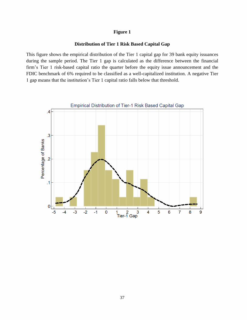
37

Figure 1

Distribution of Tier 1 Risk Based Capital Gap

This figure shows the empirical distribution of the Tier 1 capital gap for 39 bank equity issuances

during the sample period. The Tier 1 gap is calculated as the difference between the financial

firm’s Tier 1 risk-based capital ratio the quarter before the equity issue announcement and the

FDIC benchmark of 6% required to be classified as a well-capitalized institution. A negative Tier

1 gap means that the institution’s Tier 1 capital ratio falls below that threshold.

38

Figure 2

CDS Mean Spreads for the Sample Banks in the 2002-2013 Period

This figure plots the daily series of the mean CDS spreads of the 56 financial institutions that

announced equity issuances between 2002 and 2013. This sample is collected from S&P’s Capital

IQ database. We then limit the sample to those financial firms having CDS pricing data reported

by Markit. The firm provides CDS end-of-day quotes for the CDS contracts

39

Figure 3

Aggregate Market Equity Capitalization for the Sample Banks in the period 2002-2013

This figure plots the daily evolution of the combined equity market capitalization of the 56

financial institutions that announced equity issuances between 2002 and 2013. Equity market

capitalization is calculated as the daily stock price times the number of shares of common stock

outstanding (from CRSP data tapes).

40

References

Alexopoulou, I., Andersson M, Georgescu, O.M., 2009. An empirical study on the decoupling

movements between corporate bond and CDS spreads. European Central Bank, Working

Paper No. 1085.

Andenmatten, S., Brill, F., 2011. Measuring co-movements of CDS premia during the Greek

debt crisis, Discussion paper 11-04, Department of Economics, University of Bern.

Arce, O., Mayordomo, S., Pena, J.I., 2012. Credit-risk valuation in the sovereign CDS and bonds

Markets: Evidence from the Euro area crisis, available at SSRN:

http://ssrn.com/abstract=1896297.

Ballester, L., Casu, B., Gonzalez-Urteaga, A., 2013. Bank fragility and contagion: Evidence

from the CDS market, Working paper University of Valencia.

Cornett, M.M., Lei, L., Tehranian, H., 2013. The performance of banks around the receipt and

repayment of TARP funds. Journal of Banking and Finance 37, 730-746.

Cornett, M.M., Mehran, H., Tehranian, H., 1998. Are financial markets overly optimistic about

the prospects of firms that issue equity? Evidence from voluntary versus involuntary

equity issuances by banks. Journal of Finance 53, 2139-2160.

De Bruyckere, V., Gerhardt, M., Schepens, G., Vennet, R.V., 2013 Bank/sovereign risk

spillovers in the European debt crisis. Journal of Banking and Finance 37, 4793-4809.

Di Cesare, A., Guazzarotti, G., 2010. An analysis of the determinants of credit default swap

spread changes before and during the subprime financial turmoil, available at SSRN:


Demirguc-Kunt, A., Huizinga, H., 2010. Are banks too big to fail or too big to save?

International evidence from equity prices and CDS spreads. SSRN Working paper:


Eichengreen, B., Mody, A., Nedeljkovic, M., Sarno, L., 2009. How the subprime crisis went

global: Evidence from bank credit default swap spreads, NBER Working Paper No.

14904.

Flannery, M.J., Houston, J.F., Partnoy, F., 2010. Credit default swap spreads as viable substitutes

for credit ratings. University of Pennsylvania Law Review 158(7), 2085-2123.

Fontana, A., Scheicher, M., 2010. An analysis of Euro area sovereign CDS and their relation

with government bonds, available at SSRN: http://ssrn.com/abstract=1715483.

Galil, K., Shapir, O.M., Amiram, D., Ben-Zion, U., 2014. The determinants of CDS spreads.

Journal of Banking and Finance 41, 271-282.

http://ssrn.com/abstract=1896297




41

Hull, J., Predescu, M., White, A., 2004. The relationship between credit default swap spreads,

bond yields, and credit rating announcements. Journal of Banking and Finance 28, 2789-

2811.

Ismailescu, I., Kazemi, H, 2010. The reaction of emerging market credit default swap spreads to

sovereign credit rating changes. Journal of Banking and Finance 34, 2861-2873.

Jorion, P., Zhang, G., 2007. Good and bad credit contagion: Evidence from credit default swaps.

Journal of Financial Economics 84, 860-883.

Kallestrup, R., Lando, D., Murgoci, A., 2012. Financial sector linkages and the dynamics of bank

and sovereign credit spreads, available at SSRN: http://ssrn.com/abstract=2023635.

Mehran, H., Thakor, A., 2011. Bank capital and value in the cross-section. Review of Financial

Studies 24, 1019-1067.

Miller, M., 1995. Do the M&M propositions apply to banks? Journal of Banking and Finance 19,

483–489.

Ng, J., Vasvari, F.P., Wittenberg-Moerman, R., 2011. The impact of TARP’s capital purchase

program on stock market valuation of participating banks. SSRN Working paper:


Norden, L., Weber, M., 2009. The co-movement of credit default swap, bond and stock markets:

An empirical analysis. European Financial Management 15, 529-562.

Ross, S.A., 1977. The determination of financial structure: The incentive-signaling approach. Bell

Journal of Economics 8, 23-40.

Veronesi, P., Zingales, L., 2010. Paulson's gift. Journal of Financial Economics 97, 339-368.



CDS and Equity Market Reactions to Stock Issuances in … · CDS and Equity Market Reactions to...

Documents

Transcript of CDS and Equity Market Reactions to Stock Issuances in … · CDS and Equity Market Reactions to...