CCSS UG PROGRAMME MATHEMATICS (OPEN COURSE) · Chapter 1 Equations and Graphs 1.1 Equations An...
211
SCHOOL OF DISTANCE EDUCATION CCSS UG PROGRAMME MATHEMATICS (OPEN COURSE) (For students not having Mathematics as Core Course) MM5D03: MATHEMATICS FOR SOCIAL SCIENCES FIFTH SEMESTER STUDY NOTES Prepared by: Seena V. Assistant Professor Department of Mathematics Christ College, Irinjalakuda ————————————————————————————— UNIVERSITY OF CALICUT
-
Upload
nguyenkhuong -
Category
Documents
-
view
214 -
download
0
Transcript of CCSS UG PROGRAMME MATHEMATICS (OPEN COURSE) · Chapter 1 Equations and Graphs 1.1 Equations An...

SCHOOL OF DISTANCE EDUCATION
CCSS UG PROGRAMME
MATHEMATICS (OPEN COURSE)
(For students not having Mathematics as Core Course)
MM5D03: MATHEMATICS FOR SOCIAL SCIENCES
FIFTH SEMESTER
STUDY NOTES
Prepared by:
Seena V.
Assistant Professor
Department of Mathematics
Christ College, Irinjalakuda
—————————————————————————————
UNIVERSITY OF CALICUT

CCSS UG PROGRAMME
MATHEMATICS(OPEN COURSE)
(For students not having Mathematics as Core Course)
MM5D03: MATHEMATICS FOR SOCIAL SCIENCES
Study Notes
Prepared by:
Seena V.
Assistant Professor
Department of Mathematics
Christ College, Irinjalakuda
Email: [email protected]
Published by:
SCHOOL OF DISTANCE EDUCATION
UNIVERSITY OF CALICUT
August, 2013
Copy Right Reserved

Contents
1 Equations and Graphs 7
1.1 Equations . . . . . . . . . . . . . . . . . . . . . . . . . . . . . . . 7
1.2 Cartesian Coordinate System . . . . . . . . . . . . . . . . . . . . 12
1.3 Graphing Linear Equations . . . . . . . . . . . . . . . . . . . . . . 13
1.4 Solving Linear Equations Simultaneously . . . . . . . . . . . . . . 18
1.5 Slope of a Straight Line . . . . . . . . . . . . . . . . . . . . . . . 21
1.6 Solving Quadratic Equations . . . . . . . . . . . . . . . . . . . . . 24
1.7 Practical Applications of Graphs and Equations . . . . . . . . . . 29
1.8 Exercises . . . . . . . . . . . . . . . . . . . . . . . . . . . . . . . . 32
2 Functions 35
2.1 Concepts and Definitions . . . . . . . . . . . . . . . . . . . . . . . 35
2.2 Functions and Graphs . . . . . . . . . . . . . . . . . . . . . . . . 39
2.3 The Algebra of Functions . . . . . . . . . . . . . . . . . . . . . . 41
2.4 Application of Linear Functions . . . . . . . . . . . . . . . . . . . 44
2.5 Facilitating Nonlinear Graphs . . . . . . . . . . . . . . . . . . . . 45
2.6 Exercises . . . . . . . . . . . . . . . . . . . . . . . . . . . . . . . . 51
3 The Derivative 53
3.1 Limits . . . . . . . . . . . . . . . . . . . . . . . . . . . . . . . . . 53
3.2 Continuity . . . . . . . . . . . . . . . . . . . . . . . . . . . . . . . 59
3
Module-I

3.3 The Slope of a Curvilinear Function . . . . . . . . . . . . . . . . . 62
3.4 Rates of Change . . . . . . . . . . . . . . . . . . . . . . . . . . . . 66
3.5 The Derivative . . . . . . . . . . . . . . . . . . . . . . . . . . . . 70
3.6 Differentiability and Continuity . . . . . . . . . . . . . . . . . . . 73
3.7 Applications for the Social Sciences, Business, and Economics . . 74
3.8 Exercises . . . . . . . . . . . . . . . . . . . . . . . . . . . . . . . . 77
4 Differentiation 79
4.1 Derivative Notation . . . . . . . . . . . . . . . . . . . . . . . . . . 79
4.2 Rules of Differentiation . . . . . . . . . . . . . . . . . . . . . . . . 79
4.3 Higher Order Derivatives . . . . . . . . . . . . . . . . . . . . . . . 88
4.4 Higher Order Derivative Notation . . . . . . . . . . . . . . . . . . 88
4.5 Implicit Differentiation . . . . . . . . . . . . . . . . . . . . . . . . 90
4.6 Applications for Business, Economics, and Social Sciences . . . . . 92
4.7 Exercises . . . . . . . . . . . . . . . . . . . . . . . . . . . . . . . . 95
5 Uses of the Derivative 97
5.1 Increasing and Decreasing Functions . . . . . . . . . . . . . . . . 97
5.2 Concavity . . . . . . . . . . . . . . . . . . . . . . . . . . . . . . . 98
5.3 Extreme Points . . . . . . . . . . . . . . . . . . . . . . . . . . . . 101
5.4 Optimization . . . . . . . . . . . . . . . . . . . . . . . . . . . . . 102
5.5 Inflection Points . . . . . . . . . . . . . . . . . . . . . . . . . . . . 105
5.6 Curve Sketching . . . . . . . . . . . . . . . . . . . . . . . . . . . . 108
5.7 Exercises . . . . . . . . . . . . . . . . . . . . . . . . . . . . . . . . 113
6 Exponential and Logarithmic Functions 114
6.1 Exponential Functions . . . . . . . . . . . . . . . . . . . . . . . . 114
6.2 Logarithmic Functions . . . . . . . . . . . . . . . . . . . . . . . . 115
6.3 Properties of Exponents and Logarithms . . . . . . . . . . . . . . 116
6.4 Natural Exponential and Logarithmic Functions . . . . . . . . . . 118
6.5 Solving Natural Exponential and Logarithmic Functions . . . . . 122
Module-II

6.6 Derivatives of Natural Exponential and Logarithmic Functions . . 125
6.7 Logarithmic Differentiation . . . . . . . . . . . . . . . . . . . . . . 130
6.8 Practical Applications of Exponential Functions . . . . . . . . . . 131
6.9 Exercises . . . . . . . . . . . . . . . . . . . . . . . . . . . . . . . . 141
7 Integration 143
7.1 Antidifferentiation . . . . . . . . . . . . . . . . . . . . . . . . . . 143
7.2 Rules for Indefinite Integrals . . . . . . . . . . . . . . . . . . . . . 143
7.3 The Definite Integral . . . . . . . . . . . . . . . . . . . . . . . . . 149
7.4 The Fundamental Theorem of Calculus . . . . . . . . . . . . . . . 149
7.5 Properties of Definite Integrals and Area Between Curves . . . . . 151
7.6 Average Value of a Function and The Volume of a Solid of Revolution154
7.7 Practical Applications . . . . . . . . . . . . . . . . . . . . . . . . 156
7.8 Exercises . . . . . . . . . . . . . . . . . . . . . . . . . . . . . . . . 158
8 Multivariable Calculus 160
8.1 Functions of Several Variables . . . . . . . . . . . . . . . . . . . . 160
8.2 Partial Derivatives . . . . . . . . . . . . . . . . . . . . . . . . . . 161
8.3 Rules of Partial Differentiation . . . . . . . . . . . . . . . . . . . . 164
8.4 Second-Order Partial Derivatives . . . . . . . . . . . . . . . . . . 169
8.5 Optimization of Multivariable Functions . . . . . . . . . . . . . . 173
8.6 Constrained Optimization and Lagrange Multipliers . . . . . . . . 176
8.7 Total Differentials . . . . . . . . . . . . . . . . . . . . . . . . . . . 179
8.8 Exercises . . . . . . . . . . . . . . . . . . . . . . . . . . . . . . . . 181
9 More of Integration and Multivariable Calculus 183
9.1 Integration by Substitution . . . . . . . . . . . . . . . . . . . . . . 183
9.2 Integration by Parts . . . . . . . . . . . . . . . . . . . . . . . . . 187
9.3 Improper Integrals . . . . . . . . . . . . . . . . . . . . . . . . . . 190
9.4 L’Hopital’s Rule . . . . . . . . . . . . . . . . . . . . . . . . . . . . 194
9.5 Double Integrals . . . . . . . . . . . . . . . . . . . . . . . . . . . . 196

9.6 Approximating Definite Integrals . . . . . . . . . . . . . . . . . . 199
9.7 Differential Equations . . . . . . . . . . . . . . . . . . . . . . . . . 201
9.8 Separation of Variables . . . . . . . . . . . . . . . . . . . . . . . . 203
9.9 Practical Applications . . . . . . . . . . . . . . . . . . . . . . . . 205
9.10 Exercises . . . . . . . . . . . . . . . . . . . . . . . . . . . . . . . . 208

Chapter 1Equations and Graphs
1.1 Equations
An equation is a mathematical statement that two things are equal. It consists of
two expressions, one on each side of an ‘equals’sign. for example 11 = 5+ 6.This
equation states that 11 is equal to the sum of 5 and 6, which is obviously true.
In an equation, the left side is always equal to the right side.The most common
equations contain one or more variables. If we let x stand for an unknown number,
and write the equation x = 12+5. We know the left side and right side are equal,
so we can see that x must be 12+5 or 17. This is the only value that x can have
that makes the equation a true statement. We say that x = 17 ‘satisfies’the
equation. This process of finding the value of the unknowns is called solving the
equation. We often say that we “solve for x”- meaning solve the equation to find
the value of the unknown number x. Some equations have more than one solution.
If the solution set includes all real numbers, the equation is an identity. If the
solution set is empty, the equation has no solution. Two equations with identical
solution sets are referred to as equivalent. An equation in which all variables are
raised to the first power is known as a linear equation.
Example 1.1. In the mathematical expressions and statements listed below.
(a) 4x2 + 7
(b) 3x− 8 = 2y + 12
(c) 6x+ 7 = 19
7

1.1. Equations 8
(d) x2 − 3x+ 5
(e) x2 − 6x+ 5 = 5
(b), (c) and (e) are equations. (b) is an equation in two variables x and y, but
(c) is an equation in one variable x. (b) and (c) are linear equations. Note that
(e) is not linear, since power of x in (e) is two.
The same quantity Q can be added, subtracted, multiplied or divided on both
sides of the equation without effecting the equality, Q 6= 0 for division.
Properties of Equality
For all real numbers a, b, and c, if a = b,
(a) Addition Property : a+ c = b+ c
(b) Subtraction Property : a− c = b− c
(c) Multiplication Property : ac = bc
(d) Division Property : a/c = b/c (c 6= 0)
Problem 1.1. Solve the equationx
2− 3 =
x
3+ 1
Solution. Solving an equation means we have to find the values of x which
satisfies the given equation.We solve above problem in three steps.
(1) Move all terms with unknown variable to the left, here by subtractingx
3from both sides of the equation, we get
x
2− 3− x
3=
x
3+ 1− x
3(Subtraction Property)
x
2− x
3− 3 = 1
(2) Move terms without the unknown variable to the right, here by adding 3 to
both sides of the equation.
x
2− x
3− 3 + 3 = 1 + 3 (Addition Property)
School of Distance Education,University of Calicut

1.1. Equations 9
x
2− x
3= 4
(3) Simplify both sides,
x
2− x
3= 4
3 · x− 2 · x2 · 3 = 4
3x− 2x
6= 4
Multiplying by 6 we get,
6 · 3x− 2x
6= 6 · 4 (Multiplication Property)
x = 24
�
Note 1.1. Any equation which can be reduced to 0 = 0 by steps using the
properties of equality is an identity.
Note 1.2. Any equation that can be reduced to a = 0 through the properties of
equality, when a 6= 0 has no solution.
Problem 1.2. Use the properties of equality to solve the following linear equa-
tions by moving all terms with the unknown variable to the left, all other terms
to the right, and then simplifying :
(a) 4x+ 9 = 7x− 6
(b) 28− 2x = 8x− 12
(c) 9(3x+ 4)− 2x = 11 + 5(4x− 1)
Solution.
(a)
4x+ 9 = 7x− 6
4x− 7x = −6− 9
−3x = −15
x = 5
School of Distance Education,University of Calicut

1.1. Equations 10
(b)
28− 2x = 8x− 12
−2x− 8x = −12− 28
−10x = −40
x = 4
(c)
9(3x+ 4)− 2x = 11 + 5(4x− 1)
27x+ 36− 2x = 11 + 20x− 5
25x+ 36 = 6 + 20x
25x− 20x = 6− 36
5x = −30
x = −6
�
Problem 1.3. Solve the following equations:
(a) 5x− 39 = 5(x− 8) + 1
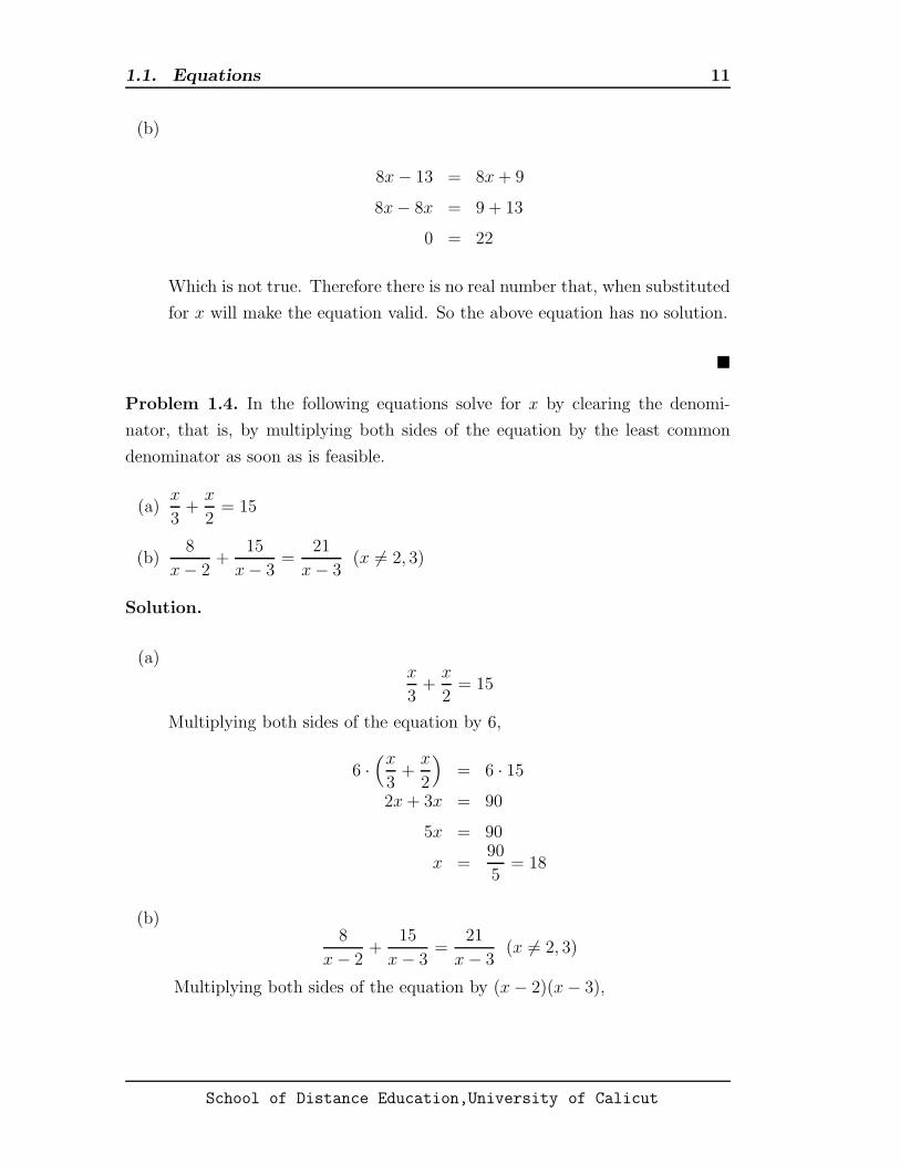
(b) 8x− 13 = 8x+ 9
Solution.
(a)
5x− 39 = 5(x− 8) + 1
5x− 39 = 5x− 40 + 1
5x− 39 = 5x− 39
5x− 5x = 39− 39
0 = 0
This means that any real number can be substituted for x and the equation
will be valid. Therefore above equation is an identity.
School of Distance Education,University of Calicut
1.1. Equations 11
(b)
8x− 13 = 8x+ 9
8x− 8x = 9 + 13
0 = 22
Which is not true. Therefore there is no real number that, when substituted
for x will make the equation valid. So the above equation has no solution.
�
Problem 1.4. In the following equations solve for x by clearing the denomi-
nator, that is, by multiplying both sides of the equation by the least common
denominator as soon as is feasible.
(a)x
3+
x
2= 15
(b)8
x− 2+
15
x− 3=
21
x− 3(x 6= 2, 3)
Solution.
(a)x
3+
x
2= 15
Multiplying both sides of the equation by 6,
6 ·(x
3+
x
2
)
= 6 · 152x+ 3x = 90
5x = 90
x =90
5= 18
(b)8
x− 2+
15
x− 3=
21
x− 3(x 6= 2, 3)
Multiplying both sides of the equation by (x− 2)(x− 3),
School of Distance Education,University of Calicut
1.2. Cartesian Coordinate System 12
(x− 2)(x− 3)
(
8
x− 2+
15
x− 3
)
=21
x− 3(x− 2)(x− 3)
8(x− 3) + 15(x− 2) = 21(x− 2)
8x− 24 + 15x− 30 = 21x− 42
23x− 54 = 21x− 42
23x− 21x = −42 + 54
2x = 12
x = 6
�
1.2 Cartesian Coordinate System
A Cartesian coordinate system in a plane is composed of horizontal line and a
vertical line set perpendicular to each other in a plane. The lines are called the
coordinate axes ; their point of intersection, the origin. The horizontal line is
generally referred to as the x-axis ; the vertical line, the y-axis. The four sections
in to which the plane is divided by the intersection of the axes are called quadrants.
Each point in the plane is uniquely associated with an ordered pair of numbers,
known as coordinates, describing the location of the point in relation to the origin.
The first coordinate, called the x-coordinate or abscissa, gives the distance of the
point from the vertical axis; the second, the y- coordinate or ordinate, gives
the distance of the point from the horizontal axis. To the right of the y-axis, x
coordinates are positive; to the left, negative. Above the x-axis, y coordinates are
positive; below, negative. The signs of the coordinates in each of the quadrants
are illustrated in the following Figure.
III
IVIII
x(+) , y(+)
x(+) , y(-)x(-) , y(-)
x(-) , y(+)
Figure 1.1
School of Distance Education,University of Calicut

1.3. Graphing Linear Equations 13
Example 1.2. The coordinates give the location of the point P in relation to the
origin. The point (4, 3) is four units to the right of the y- axis, three units above
the x- axis. P (−4, 3) is four units to the left of the y- axis, three units above the
x- axis. P (−4,−3) is four units to the left of the y- axis, three units below the
x- axis; P (4,−3) is four units to the right of the y- axis, three units below the x-
axis. See Figure 1.2.
0 x
y
1 2 3 4
(4,3)
-1-2-3-4
(-4,-3)
1
2
3
4
-1
-2
-3
-4
(-4,3)
(4,-3)
Figure 1.2
1.3 Graphing Linear Equations
For any equation in x and y, one can isolate a set of points in the Cartesian
coordinate system. The set of points is called the graph of the equation. The
graph of a linear equation is a straight line.
The x-intercept is the point where the graph crosses the x- axis ; the y-
intercept is the point where the graph crosses the y- axis. Since the line crosses
the x- axis where y = 0, the y-coordinate of the x-intercept is always 0. The
x- coordinate of the x-intercept is then obtained simply by setting y equal to
zero and solving the equation for x. Similarly the line crosses the y- axis where
x = 0, the x-coordinate of the y-intercept is always 0. The y- coordinate of the
y-intercept is then obtained simply by setting x equal to zero and solving the
equation for y.
The slope-intercept form of a line is given by
y = mx+ b (m, b = constants)
where m is the slope of the line and (0, b) is the y- intercept. The y-coordinate of
the y-intercept is always a constant in the slope-intercept form of the equation.
School of Distance Education,University of Calicut

1.3. Graphing Linear Equations 14
Problem 1.5. Put the following linear equations in to the slope-intercept form
by solving for y in terms of x and /or a constant:
(a) 40x+ 8y = 96
(b) 18x− 9y = 27
(c) 63x− 7y = 0
Solution.
(a)
40x+ 8y = 96
8y = 96− 40x
8y = −40x+ 96
y = −5x+ 12(b)
18x− 9y = 27
−9y = 27− 18x
−9y = −18x+ 27
y = −2x+ 3(c)
63x− 7y = 0
−7y = −63x
y = 9x
�
Problem 1.6. Find the y-intercept for each of the following equations :
(a) 3x+ y = 7
(b) 9x− 3y = 72
(c) y = 24x− 45
School of Distance Education,University of Calicut
1.3. Graphing Linear Equations 15
Solution.
(a) The y-intercept occurs where the line crosses the y-axis, which is the point
where x = 0 . Setting x = 0 in the equation 3x + y = 7 and solving for y
we have,
3(0) + y = 7
y = 7
Hence the y-intercept is (0, 7)
(b) Setting x = 0,
9(0)− 3y = 72
−3y = 72
y = −24
Hence the y-intercept is (0,−24)
(c) Here the equation is in the slope-intercept form. Hence the y-intercept is
(0,−45).
�
Problem 1.7. Find the x-intercept for each of the following equations :
(a) y = 6x− 54
(b) y = 12x+ 132
Solution.
(a) The x-intercept is the point where the line crosses the x-axis, which is the
point where y = 0 . Setting y = 0 in the equation y = 6x− 54 and solving
for x, we have
0 = 6x− 54
−6x = −54
x = 9
Hence the x-intercept is (9, 0)
School of Distance Education,University of Calicut

1.3. Graphing Linear Equations 16
(b) Setting y = 0,
0 = 12x+ 132
−12x = 132
x = −11
Hence the x-intercept is (−11, 0).
�
Problem 1.8. Find the x-intercept in terms of the parameters of the slope-
intercept form of a linear eqauation y = mx+ b
Solution. Setting y = 0,
0 = mx+ b
−mx = b
x = − b
m(1.1)
Hence the x-intercept of the slope intercept form is (−b/m, 0) �
Problem 1.9. Use the information in Problem 1.8 to speed the process of finding
the x-intercepts for the following equations :
(a) y = 15x+ 75
(b) y = 25x+ 225
Solution.
(a) Here m = 15, b = 75. Substituting in (1.1),
x = −75
15= −5
So the x-intercept is (−5, 0).
(b) Here m = 25, b = 225. Substituting in (1.1),
x = −225
25= −9
So the x-intercept is (−9, 0). �
School of Distance Education,University of Calicut

1.3. Graphing Linear Equations 17
Problem 1.10. Find the y-intercepts and x-intercepts and use them as the two
points needed to graph the following linear equations:
(a) y = −4x+ 8
(b) y = 2x+ 4
(c) y = 2
Solution.
(a) y-intercept is (0, 8) and x-intercept is (2, 0)
0 x
y
1 2 3 4
4
5
2
6y = - 4x + 8
8
Figure 1.3
(b) y-intercept is (0, 4) and x-intercept is (−2, 0)
0 x
y
1 2 3 4
4
5-1- 2-3
1
2
3
y = 2x+4
Figure 1.4
School of Distance Education,University of Calicut

1.4. Solving Linear Equations Simultaneously 18
(c) y-intercept is (0, 2) , x-intercept does not exist because y cannot be set
equal to zero without involving contradiction. Since y = 2 independently
of x, y will equal to 2 for any value of x.
0 x
y
1 2 3 4
4
5-1- 2-3
1
2
3 y = 2
Figure 1.5
�
1.4 Solving Linear Equations Simultaneously
Two equations involving the same two variables can be solved algebraically or
graphically. To solve algebraically (1) express the equations in the slope intercept
form, (2) equate the two expressions for y and solve for x, and then (3) substitute
the solution for x in either of the equations to find y. To solve graphically, graph
the two equations on the same plane and look for the point of intersection . The
coordinates of the point of intersection, represents the unique point common to
both equations, provide the solution.
Problem 1.11. Solve each of the following systems of equations algebraically.
(a) −5x+ y = −8; 6x− y = 11
(b) 6x+ 2y = 16; −4x+ y = −6
Solution.
(a) (1) Setting each of the equations in slope-intercept form,
y = 5x− 8
y = 6x− 11
School of Distance Education,University of Calicut

1.4. Solving Linear Equations Simultaneously 19
(2) Equating y’s and solving for x,
5x− 8 = 6x− 11
5x− 6x = −11 + 8
−x = −3
x = 3
(3) Substituting x = 3 in either of the equations,
y = 5(3)− 8
y = 15− 8
y = 7
Hence the solution is x = 3, y = 7.
(b) (1) Setting each of the equations in slope-intercept form,
y = −3x+ 8
y = 4x− 6
(2) Equating y’s and solving for x,
−3x+ 8 = 4x− 6
−3x− 4x = −6− 8
−7x = −14
x = 2
(3) Substituting x = 2 in either of the equations,
y = −3(2) + 8
y = −6 + 8
y = 2
Hence the solution is x = 2, y = 2. �
School of Distance Education,University of Calicut

1.4. Solving Linear Equations Simultaneously 20
Problem 1.12. Solve each of the following system of equations graphically:
(a) y = −2x+ 10; y = 14x+ 1
(b) y = −15x+ 3; y = 2x− 8
Solution.
(a) For the line y = −2x + 10, x-intercept is (5, 0) and y- intercept is (0, 10).
For y = 14x+ 1, x-intercept is (−4, 0) and y- intercept is (0, 1).
0 x
y
1 2 3 4-1-2-3-4
1
2
3
4
5 6-5
6
5
10
9
8
7
(4,2)
y = - 2x + 10
y = 1/4 x + 1
Figure 1.6
From Figure the point of intersection is (4, 2).So the solution is x = 4, y = 2.
(b) Intercepts : (0, 3), (15, 0); (0,−8), (4, 0)
0
y
2 4 6 8-1
-2
-3
-4
1
2
3
4
10
-6
-5
(5,2)
x
-8
-7
161412
y = 2x - 8
y = -1/5 x + 3
Figure 1.7
From Figure the point of intersection is (5, 2). So the solution is x = 5, y =
2.
School of Distance Education,University of Calicut

1.5. Slope of a Straight Line 21
1.5 Slope of a Straight Line
The slope indicates the steepness and direction of a line. The slope of a horizontal
line y = k ( a constant) is zero. The slope of a vertical line x = a (a constant) is
undefined.
For a line passing through the points (x1, y1) and (x2, y2), the slope
m =y2 − y1x2 − x1
=y1 − y2x1 − x2
(x1 6= x2)
A line with slope m and passing through the point (x1, y1) has the equation,
called the point-slope form
y − y1 = m(x− x1)
Problem 1.13. Find the slope of the lines represented by the following lines:
(a) y = −7x+ 13
(b) y = 5x+ 3
(c) 15x+ 5y = 40
(d) 8x− 2y = 28
Solution.
(a) In the slope-intercept form of a linear equation, the coefficient of x is the
slope of the line. The given equation is in slope-intercept form, so its slope
is −7.
(b) The given equation is in slope-intercept form, so its slope is coefficient of x
which is equal to 5.
(c) First convert the given equation in to slope-intercept form,
15x+ 5y = 40
5y = 40− 15x
5y = −15x+ 40
y = −3x+ 8
School of Distance Education,University of Calicut

1.5. Slope of a Straight Line 22
The slope intercept form of given equation is y = −3x + 8, so its slope is
−3.
(d) First convert the given equation in to slope-intercept form,
8x− 2y = 28
−2y = 28− 8x
−2y = −8x+ 28
y = 4x− 14
The slope intercept form of given equation is y = 4x− 14, so its slope is 4.
�
Problem 1.14. Find the slope of the line passing through the points (2, 3) and
(5, 12).
Solution. Let (x1, y1) = (2, 3) and (x2, y2) = (5, 12). The slope
m =y2 − y1x2 − x1
=12− 3
5− 2=
9
3= 3.
So the slope of the line passing through the points (2, 3) and (5, 12) is 3. �
Problem 1.15. Find the slope of the line passing through the points (1, 7) and
(5, 15).
Solution. Let (x1, y1) = (1, 7) and (x2, y2) = (5, 15). The slope
m =y2 − y1x2 − x1
=15− 7
5− 1=
8
4= 2.
So the slope of the line passing through the points (1, 7) and (5, 15) is 2. �
Problem 1.16. Find the equation of the line passes through the point (3, 10)
and has slope −4.
Solution. Let (x1, y1) = (3, 10), given slope m = −4. Then equation of the line
is,
y − y1 = m(x− x1)
School of Distance Education,University of Calicut

1.5. Slope of a Straight Line 23
y − 10 = −4(x− 3)
y − 10 = −4x+ 12
y = −4x+ 12 + 10
y = −4x+ 22
�
Problem 1.17. Find the equation of the line passes through the point (−8, 2)
and has slope 3.
Solution. Let (x1, y1) = (−8, 2), given slope m = 3. Then the equation of the
line is,
y − y1 = m(x− x1)
y − 2 = 3(x− (−8))
y − 2 = 3(x+ 8)
y − 2 = 3x+ 24
y = 3x+ 24 + 2
y = 3x+ 26
�
Problem 1.18. Find the equation for the line passing through (−2, 5) and par-
allel to the line having the equation y = 3x+ 7.
Solution. Parallel lines have the same slope . The slope of the line y = 3x+ 7
is 3. So we have to find the equation for the line passing through (−2, 5) with
slope 3. Let (x1, y1) = (−2, 5), here slope m = 3. Then the equation of the line
is,
y − y1 = m(x− x1)
y − 5 = 3(x− (−2))
y − 5 = 3x+ 6
y = 3x+ 6 + 5
y = 3x+ 11
�
School of Distance Education,University of Calicut
1.6. Solving Quadratic Equations 24
Problem 1.19. Find the equation for the line passing through (8, 3) and per-
pendicular to the line having the equation y = 4x+ 13.
Solution. Perpendicular lines have slopes that are negative reciprocals of one
another. The slope of the line y = 4x+ 13 is 4, the slope of a line perpendicular
to it must be −14. So we have to find the equation for the line passing through
(8, 3) with slope −14. Let (x1, y1) = (8, 3), here slope m = −1
4. Then the equation
of the line is,
y − y1 = m(x− x1)
y − 3 = −1
4(x− 8)
y − 3 = −1
4x+ 2
y = −1
4x+ 2 + 3
y = −1
4x+ 5
�
1.6 Solving Quadratic Equations
An equation of the form ax2+bx+c = 0 where a, b, and c are constants and a 6= 0
is called a quadratic equation. Quadratic equations can be solved by factoring,
completing the square or using the quadratic formula
x =−b±
√b2 − 4ac
2a(1.2)
Factoring is the reverse process of multiplication by which a polynomial is ex-
pressed as a product of simpler polynomials called factors.
Note 1.3. Let p and q be two integers such that p = a + b and q = ab for some
integers a, b. Then we can write x2 + px+ q as (x+ a)(x+ b).
Note 1.4. An expression in the form x2 + bx can be converted in to perfect
square by adding the square of the half of the coefficient of x, that is
(
b
2
)2
to
the original expression. Thus we get x2 + bx+
(
b
2
)2
=
(
x+b
2
)2
School of Distance Education,University of Calicut
1.6. Solving Quadratic Equations 25
Problem 1.20. Solve the following quadratic equations by factoring:
(a) x2 + 12x+ 35 = 0
(b) x2 − 4x− 32 = 0
Solution.
(a) Comparing the given equation with x2 + px+ q we get p = 12 and q = 35,
that is, a + b = 12 and ab = 35. The numbers that satisfies above two
equations are 7 and 5. So,
x2 + 12x+ 35 = (x+ 5)(x+ 7) = 0
⇒ (x+ 5) = 0 or (x+ 7) = 0
⇒ x = −5 or x = −7
So solution of x2 + 12x+ 35 = 0 is x = −5,−7.
(b) Comparing the given equation with x2+px+q we get p = −4 and q = −32,
that is, a + b = −4 and ab = −32. The numbers that satisfies above two
equations are -8 and 4. So,
x2 − 4x− 32 = (x+ 4)(x− 8) = 0
⇒ (x+ 4) = 0 or (x− 8) = 0
⇒ x = −4 or x = 8
So solution of x2 − 4x− 32 = 0 is x = −4, 8.
�
Problem 1.21. Solve the following quadratic equations using the quadratic formula:
(a) 3x2 + 20x+ 12 = 0
(b) 11x2 + x− 12 = 0
School of Distance Education,University of Calicut

1.6. Solving Quadratic Equations 26
Solution. Using 1.2 and substituting a = 3, b = 20, and c = 12,
x =−b±
√b2 − 4ac
2a
=−20±
√
(20)2 − 4(3)(12)
2(3)
=−20±
√400− 144
6
=−20±
√256
6
=−20± 16
6
x =−20 + 16
6=
−4
6=
−2
3, x =
−20− 16
6=
−36
6= −6.
�
Problem 1.22. Complete the square and write the following expressions as per-
fect squares :
(a) x2 + 6x
(b) x2 − 14x
(c) x2 − 6
5
Solution.
(a) Comparing given equation with the equation x2 + bx, we get b = 6,
b
2=
6
2= 3 and
(
b
2
)2
= 32 = 9. Adding 9 to the original expression and
factoring,
x2 + 6x+ 9 = (x+ 3)2
(b) Comparing given equation with the equation x2 + bx, we get b = −14,
b
2=
−14
2= −7 and
(
b
2
)2
= (−7)2 = 49. Adding 49 to the original
expression and factoring,
x2 − 14x+ 49 = (x− 7)2
School of Distance Education,University of Calicut

1.6. Solving Quadratic Equations 27
(c) Comparing given equation with the equation x2 + bx, we get b =−6
5,
b
2=
−6
5 · 2 =−3
5and
(
b
2
)2
=
(−3
5
)2
=9
25. Adding
9
25to the original
expression and factoring,
x2 − 6
5x+
9
25=
(
x− 3
5
)2
�
Problem 1.23. Use the process of completing the square to solve the following
quadratic equations:
(a) x2 + 12x+ 32 = 0
(b) x2 − 10x+ 13 = 0
(c) −x2 + 8x+ 20 = 0
(d) 3x2 + 24x+ 30 = 0
Solution.
(a) Move the constant term to the right-hand side we get,
x2 + 12x = −32
Ignore the constant for the moment and complete the square on the left as
in Problem 1.22, getting b = 12,12
2= 6 and 62 = 36. Now add 36 to both
sides of the equation to keep the equality,
x2 + 12x+ 36 = −32 + 36
Next factor the left-hand side to obtain the perfect square,
(x+ 6)2 = 4
Take the square root of both sides of the equation and solve for x,
x+ 6 = ±√4
x = −6 ±√4
x = −6 ± 2
School of Distance Education,University of Calicut
1.6. Solving Quadratic Equations 28
⇒ x = −6 + 2 = −4, x = −6− 2 = −8.
(b) Moving the constant term to the right-hand side we get,
x2 − 10x = −13
Here b = −10,−10
2= −5 and (−5)2 = 25. Now add 25 to both sides of the
equation to keep the equality,
x2 − 10x+ 25 = −13 + 25
Next factor the left-hand side to obtain the perfect square,
(x− 5)2 = 12
Take the square root of both sides of the equation and solve for x,
x− 5 = ±√12
x = 5±√12
x = 5± 2√3
⇒ x = 5 + 2√3, x = 5− 2
√3
(c) Here coefficient of x2 is -1, so we first factoring out -1. Then our equation
become
x2 − 8x− 20 = 0
Moving the constant term to the right-hand side we get,
x2 − 8x = 20
Here b = −8,−8
2= −4 and (−4)2 = 16. Adding 16 and solving,
x2 − 8x+ 16 = 20 + 16
(x− 4)2 = 36
x− 4 = ±√36
x = 4±√36
x = 4± 6
School of Distance Education,University of Calicut

1.7. Practical Applications of Graphs and Equations 29
⇒ x = 4 + 6 = 10, x = 4− 6 = −2.
(d) Here coefficient of x2 is 3, factoring out 3. Then our equation become
x2 + 8x+ 10 = 0
Moving the constant term to the right-hand side we get,
x2 + 8x = −10
Here b = 8,8
2= 4 and (4)2 = 16. Adding 16 and solving,
x2 + 8x+ 16 = −10 + 16
(x+ 4)2 = 6
x+ 4 = ±√6
x = −4 ±√6
⇒ x = −4 +√6, x = −4 −
√6
�
1.7 Practical Applications of Graphs and Equa-
tions
Problem 1.24. A firm has a fixed cost of $ 4,000 for plant and equipment and
an extra or marginal cost of $ 300 for each additional unit produced. What is its
total cost, C, of producing
(a) 25 units of output.
(b) 40 units of output.
Solution. Fixed cost is $4,000 and cost for producing one additional unit is $300.
So total cost for producing x unit is
C = 300x+ 4, 000
School of Distance Education,University of Calicut
1.7. Practical Applications of Graphs and Equations 30
(a) If x = 25, C = 300(25) + 4, 000 = 11, 500
(b) If x = 40, C = 300(40) + 4, 000 = 16, 000
Problem 1.25. A firm operating in pure competition receives $25 for each unit
of output sold. It has a marginal cost of $15 per item and a fixed cost of $1,200.
What is its profit level, π, if it sells
(a) 200 items.
(b) 300 items.
(c) 100 items.
Solution.
profit(π) = revenue(R)− cost(C)
Here revenue R = 25x and C = 15x+ 1, 200
Substituting we get,
π = 25x− (15x+ 1, 200) = 10x− 1, 200
(a) at x = 200, π = 10(200)− 1, 200 = 800
(b) at x = 300, π = 10(300)− 1, 200 = 1, 800
(c) at x = 100, π = 10(100)− 1, 200 = −200 (a loss)
�
Problem 1.26. For tax purpose the value y of a factory after x years is
y = 9, 000, 000− 850, 000x
(a) The value after 4 years.
(b) The salvage value after 9 years.
Solution.
(a) y = 9, 000, 000− 850, 000(4) = 5, 600, 000
(b) y = 9, 000, 000− 850, 000(9) = 1, 350, 000 �
School of Distance Education,University of Calicut

1.7. Practical Applications of Graphs and Equations 31
Problem 1.27. Find the break-even point for the firm operating in pure com-
petition, given that total revenue is R = 25x and total cost is C = 15x+ 1200.
Note 1.5. At the break-even point total revenue just equals total cost. So at
break-even point profit is zero.
At break-even point,
R = C
25x = 15x+ 1200
25x− 15x = 1200
10x = 1200
x = 120
Problem 1.28. Find the break-even for a firm operating on monopolistic com-
petition, given that total revenue is R = 48x−x2 and total cost is TC = 6x+120.
The break-even occurs when
R = TC
48x− x2 = 6x+ 120
0 = 6x+ 120− 48x+ x2
0 = 120− 42x+ x2
⇒ x2 − 42x+ 120 = 0
⇒ x =−(−42)±
√
(−42)2 − 4(1)(120)
2(1)
=42±
√1764− 480
2
=42±
√1284
2
=42± 2 ·
√321
2
= 21±√321
⇒ x = 21 +√321, x = 21−
√321
So break- even points are x = 21 +√321, x = 21−
√321
School of Distance Education,University of Calicut
1.8. Exercises 32
Problem 1.29. Find the equilibrium price p0 and quantity q0 given Supply :
q = 30p− 280 and Demand : q = −16p+ 410.
Note 1.6. Equilibrium price is the market price at which the supply of an item
equals the quantity demanded.
Equating supply and demand for equilibrium and solving for p,
30p− 280 = −16p+ 410
30p+ 16p = 410 + 280
46p = 690
p =690
46= 15
So equilibrium price p0 = 15. Substitute p0 either in supply or in demand to find
q0.
q0 = 30(15)− 280 = 170.
1.8 Exercises
1. Solve the following equations
(a) 2x+ 5 = 5x− 4
(b) 10x− 45 = 5(2x− 12) + 15
(c)x
3− 16 =
x
12+ 14
(d)48
x− 5− 45
x=
28
x− 5(x 6= 5)
2. In the following equations solve for x by clearing the denominator, that is,
by multiplying both sides of the equation by the least common denominator
as soon as is feasible.
(a)x
3− 16 =
x
12+ 14
(b)5
x+
3
x+ 4=
7
x(x 6= 0,−4)
(c)48
x− 5− 45
x=
28
x− 5(x 6= 0, 5)
School of Distance Education,University of Calicut
1.8. Exercises 33
3. Solve each of the following systems of equations algebraically:
(a) 12x+ y = 7; x+ 3y = 15
(b) 7x− y = 3; 5x+ y = 2
(c) −8x+ 2y = 10; 23x− 1
3y = 1
4. Find the y-intercepts and x-intercepts and use them as the two points
needed to graph the following linear equations:
(a) y = 3x− 9
(b) y = 14x− 2
(c) y = 3x
5. Solve each of the following systems of equations graphically.
(a) y = −2x+ 10; y = 6x+ 2
(b) 2x− y = 8; 9x+ 3y = 21
(c) 5x+ y = 15; 2x− y = −1
6. Find the slope of the lines represented by the following lines
(a) y = 13x− 5
(b) y = −9x
(c) y = 15
(d) x = 4
(e) 12y − 30x = 60
(f) 18x− 8y = 4
7. Find the slope of the line passing through the following points.
(a) (3, 11) and (6, 2)
(b) (−9,−14) and (−5,−4)
8. Write an equation for each of the lines below:
(a) Line passing through (−8, 2) with slope 3
(b) Line passing through (6,−4) with slope 12
School of Distance Education,University of Calicut

1.8. Exercises 34
9. Solve the following quadratic equations by factoring:
(a) x2 + 13x+ 40 = 0
(b) x2 + 31x− 66 = 0
10. Solve the following quadratic equations using the quadratic formula:
(a) 5x2 + 31x+ 30 = 0
(b) 7x2 − 28x+ 28 = 0
11. Use the process of completing the square to solve the following quadratic
equations:
(a) x2 − 6x− 27 = 0
(b) x2 − 18x+ 76 = 0
(c) −5x2 − 30x+ 25 = 0
(d) 11x2 + x− 12 = 0
12. A firm has a fixed cost of $1,500 for plant and equipment and an extra or
marginal cost of $200 for each additional unit produced. What is its total
cost, C, of producing
(a) 15 units of output.
(b) 20 units of output.
13. Find the profit level of a firm in pure competition that has fixed cost of
$750, a marginal cost of $80, and selling price of $95 when it sells
(a) 40 units.
(b) 60 units.
14. Find the equilibrium price p0 and quantity q0 given Supply : q = 200p−1400
and Demand : q = −50p+ 1850.
School of Distance Education,University of Calicut

Chapter 2Functions
2.1 Concepts and Definitions
A function from a set A in to a set B is a rule that assigns each elements in a set
A to exactly one element in a set B. The set A is called the domain of a function
(the set of input) and the set B is called the range of the function. (the set of
output) Usually we will denote it by y = f(x), where x is the input and is called
the independent variable and y is the output and is called the dependent variable.
f(x) we read as “f of x”or the “value of f at x”. The domain of a function refers
to the set of all possible values for the independent variable; the range refers to
the set of all possible values for the dependent variable.
Example 2.1. The function
f(x) =x
2+ 7
is the rule that takes a number, divides it by 2, and then adds 7 to the quotient.
If a value is given for x, the value is substituted for x in the formula and the
equation solved for f(x). For example, if x = 4, f(4) =4
2+ 7 = 9. If x = 6,
f(6) =6
2+ 7 = 10.
Example 2.2. If x represents the speed limit in miles per hour, then the speed
limit in kilometers per hour is a function of x, represented by f(x) = 1.6094x. If
the speed limit in the United States is 55 mi/h, its kilometre equivalent, when
rounded to the nearest integer is,
f(55) = 1.6094(55) = 89 km/h
35

2.1. Concepts and Definitions 36
Some important functions
Linear function: f(x) = mx+ b
Quadratic function : f(x) = ax2 + bx+ c (a 6= 0)
Polynomial function of degree n :
f(x) = anxn + an−1x
n−1 + · · ·+ a1x+ a0 (n = non negative integer; an 6= 0)
Rational function: f(x) =g(x)
h(x)where g(x) and h(x) are both polynomials and h(x) 6= 0
Power function : f(x) = axn (n = any real number )
The domain of linear, quadratic, and polynomial functions is the set of all real
numbers; the domain of rational and power functions excludes any value of x
involving an undefined operation.
Example 2.3. Listed below are examples of different functions:
Linear : f(x) = 3x+ 2, g(x) = −5x, h(x) = 8
Quadratic : f(x) = 5x2 + 4x+ 3, g(x) = x2 − 4x, h(x) = 4x2
Polynomial : f(x) = 4x3 + 2x2 − 9x+ 5, g(x) = 2x5 − x3 + 7
Rational : f(x) =x2 − 9
x+ 4, g(x) =
5x
x− 2(x 6= −4, 2)
Power: f(x) = 2x6, g(x) = 4x−3
Problem 2.1. .
(a) Given f(x) = x2 + 5x− 6, find f(3) and f(−4).
(b) Given f(x) =4x2 − 9x+ 17
x+ 7, find f(5) and f(−3).
(c) Given f(x) =x2 − 11
x+ 4, find f(a) and f(a− 5).
Solution.
(a) Substituting 3 for each occurrence of x in the function, we have
f(3) = (3)2 + 5(3)− 6 = 18
School of Distance Education,University of Calicut
2.1. Concepts and Definitions 37
Now substituting -4 for each occurrence of x,
f(−4) = (−4)2 + 5(−4)− 6 = −10
(b) Substituting 5 for each occurrence of x in the function, we have
f(5) =4(5)2 − 9(5) + 17
5 + 7=
72
12= 6
Now substituting -3 for each occurrence of x,
f(−3) =4(−3)2 − 9(−3) + 17
(−3) + 7=
80
4= 20
(c) Substituting a for each occurrence of x in the function, we have
f(a) =a2 − 11
a+ 4
Now substituting (a− 5) for each occurrence of x,
f(a− 5) =(a− 5)2 − 11
(a− 5) + 4=
a2 − 10a+ 14
a− 1
�
Problem 2.2. Which of the following equations are functions and why?
(a) y = −2x+ 7
(b) y2 = x
(c) x = 4
(d) −x2 + 6x+ 15
(e) y = x2
(f) x2 + y2 = 36
Solution.
(a) y = −2x+7 is a function because for each value of the independent variable
x there is one and only one value of the dependent variable y.
School of Distance Education,University of Calicut
2.1. Concepts and Definitions 38
(b) y2 = x, which is equivalent to y = ±√x is not a function because for each
positive value of x there are two values of y. For example, if y2 = 4 then
y = ±2.
(c) x = 4 is not a function. The graph of x = 4 is vertical line. This means
that at x = 4, y has many values.
(d) y = −x2 + 6x + 15 is a function because for each value of the variable x
there is a unique value of y.
(e) y = x2 is a function. Because for each value of the variable x there is a
unique value of y.
(f) x2 + y2 = 36 is not a function. If x = 0, y2 = 36 and y = ±6.
�
Problem 2.3. Identify the domain of the following functions:
(a) y = 4x2 + 7x− 19
(b) y =√t− 5
(c) y =7
x(x− 4)
(d) y =6x
(x− 5)(x− 9)
Solution.
(a) The domain of a function is the set of all acceptable values of the inde-
pendent variable. Since x may assume any value in (a), the domain of the
function is the set of all real numbers.
(b) A square root is defined only for non negative numbers (that is , x ≥ 0),
it is necessary that t − 5 ≥ 0, that is t ≥ 5. So domain of the function is
{t : t ≥ 5}.
(c) Because division by zero is not permissible, x(x−4) cannot equal zero. The
domain of the function excludes x = 0 and x = 4. So the domain of the
function is {x : x 6= 0, 4}.
School of Distance Education,University of Calicut

2.2. Functions and Graphs 39
(d) Because division by zero is not permissible, (x−5)(x−9) cannot equal zero.
The domain of the function excludes x = 5 and x = 9. So the domain of
the function is {x : x 6= 5, 9}.
�
Problem 2.4. Identify the range of the following functions:
(a) y = 2x
(b) y = x2
(c) y = 3x− 2 (−2 ≤ x ≤ 2)
Solution.
(a) The range of a function is the set of all possible values of the dependent
variable y. Here the range is the set of all real numbers since the domain
includes all real numbers.
(b) Since the square of a number cannot be negative, the range includes all non
negative numbers (that is y ≥ 0).
(c) The range of y is (−8 ≤ y ≤ 4).
�
2.2 Functions and Graphs
The graph of a linear function is a straight line.To graph a nonlinear function,
simply pick some representative value of x; solve for f(x), which is usually referred
to as y in graphing; plot the resulting ordered pairs (x, f(x)); and connect them
with a smooth line.
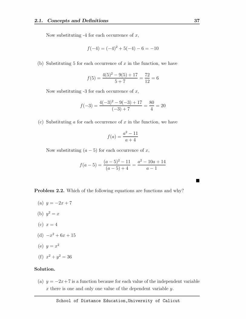
Problem 2.5. Plot the graph of y = x2.
Solution.
x -3 -2 -1 0 1 2 3
f(x) = x2 9 4 1 0 1 4 9
School of Distance Education,University of Calicut
2.2. Functions and Graphs 40
0 x
y
1 2 3 4-1-2-3-4
1
2
3
4
5 6-5
6
5
10
9
8
7
y = x2
Figure 2.1
�
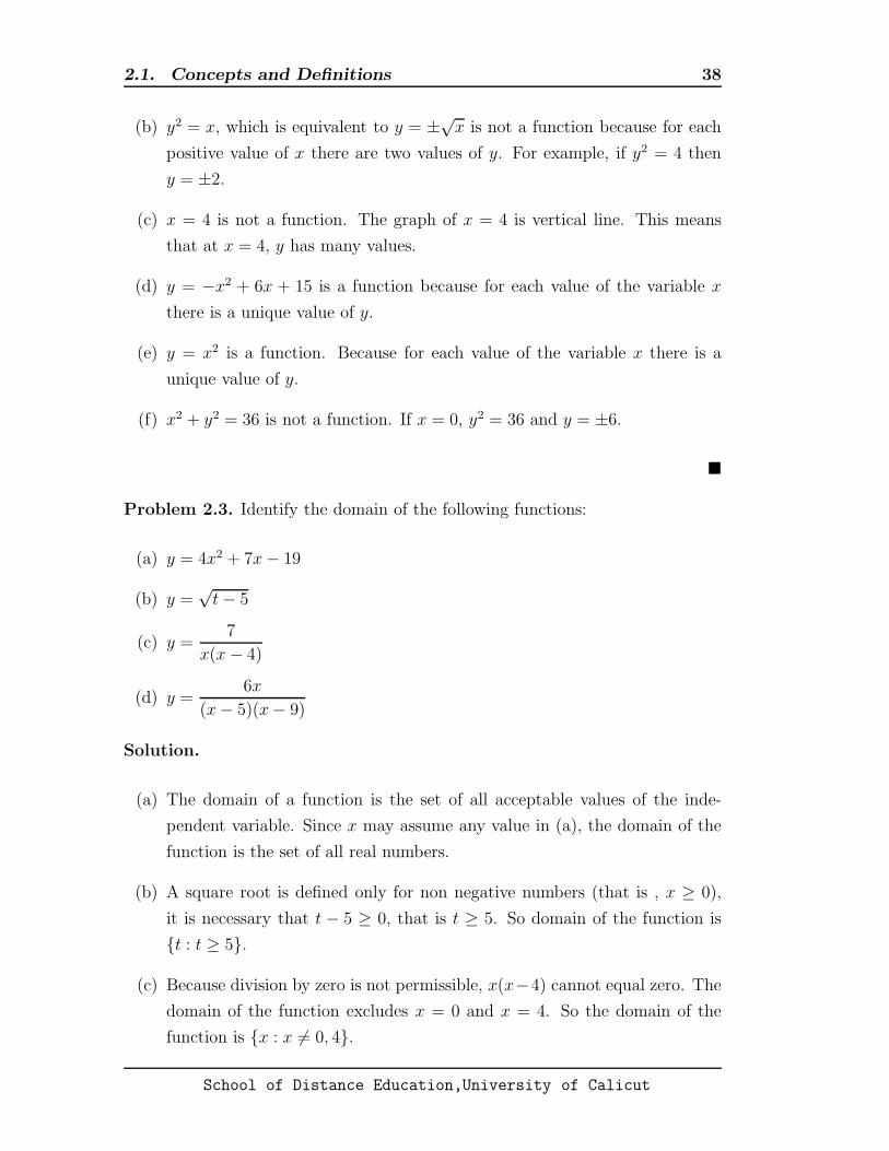
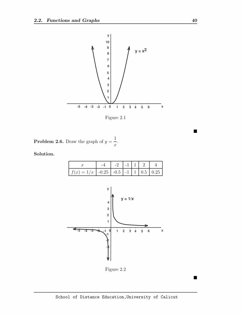
Problem 2.6. Draw the graph of y =1
x.
Solution.
x -4 -2 -1 1 2 4
f(x) = 1/x -0.25 -0.5 -1 1 0.5 0.25
0 x
y
1 2 3 4-1-2-3-4
1
2
3
4
5 6-5-1
-2
-3
y = 1/x
Figure 2.2
�
School of Distance Education,University of Calicut
2.3. The Algebra of Functions 41
The graph of a quadratic function of the form f(x) = ax2 + bx+ c, where a 6= 0,
is a parabola. The graph of a parabola is symmetric about a line called the axis
of symmetry. The point of intersection of the parabola and its axis is called the
vertex. In Figure 2.1, the axis coincides with the y-axis; the vertex is (0, 0).
2.3 The Algebra of Functions
Two or more functions can be combined to obtain a new function by addition,
subtraction, multiplication, or division of the original functions. Given two func-
tions f and g , with x in the domain of both f and g,
(f + g)(x) = f(x) + g(x)
(f − g)(x) = f(x)− g(x)
(f · g)(x) = f(x) · g(x)(f ÷ g)(x) = f(x)÷ g(x) [g(x) 6= 0]
Functions can also be combined by substituting one function f(x) for every occur-
rence of x in another function g(x). This is known as a composition of functions
and is denoted by g[f(x)] or (g ◦ f)(x).
Problem 2.7. If f(x) = 5x+ 3 and g(x) = 4x− 8, then find (f + g)(x),
(f − g)(x), (f · g)(x) and (f ÷ g)(x).
Solution. We have,
(f + g)(x) = f(x) + g(x)
(f + g)(x) = (5x+ 3) + (4x− 8) = 9x− 5
(f − g)(x) = f(x)− g(x)
(f − g)(x) = (5x+ 3)− (4x− 8) = x+ 11
(f · g)(x) = f(x) · g(x)(f · g)(x) = (5x+ 3) · (4x− 8) = 20x2 − 28x− 24
(f ÷ g)(x) = f(x)÷ g(x) [g(x) 6= 0]
(f ÷ g)(x) =(5x+ 3)
(4x− 8)(x 6= 2)
�
School of Distance Education,University of Calicut

2.3. The Algebra of Functions 42
Problem 2.8. If f(x) =4
xand g(x) =
3
x+ 2, then find (f + g)(x), (f − g)(x),
(f · g)(x) and (f ÷ g)(x).
Solution.
(f + g)(x) =4
x+
3
x+ 2=
4(x+ 2) + 3x
x(x+ 2)=
4x+ 8 + 3x
x2 + 2x=
7x+ 8
x2 + 2x
(f − g)(x) =4
x− 3
x+ 2=
4(x+ 2)− 3x
x(x+ 2)=
4x+ 8− 3x
x2 + 2x=
x+ 8
x2 + 2x
(f · g)(x) =4
x· 3
x+ 2=
12
x(x+ 2)=
12
x2 + 2x
(f ÷ g)(x) =4
x÷ 3
x+ 2=
4
x· x+ 2
3=
4(x+ 2)
3x=
4x+ 8
3x
�
Problem 2.9. If f(x) =3x
x+ 5, g(x) =
x− 4
x+ 1and h(x) =
x+ 6
x− 2,
where (x 6= −5,−1, 2) find :
(a) (f + h)(a)
(b) (h− f)(x+ 1)
Solution.
(a) (f + h)(a) = f(a) + h(a). Substituting a for each occurrence of x,
(f + h)(a) =3a
a + 5+
a + 6
a− 2
=3a(a− 2) + (a+ 6)(a+ 5)
(a + 5)(a− 2)
=3a2 − 6a+ a2 + 6a+ 5a + 30
a2 + 5a− 2a− 10
=4a2 + 5a+ 30
a2 + 3a− 10
School of Distance Education,University of Calicut

2.3. The Algebra of Functions 43
(b) (h− f)(x+1) = h(x+1)− f(x+1). Substituting x+1 for each occurrence
of x,
(h− f)(x+ 1) =(x+ 1) + 6
(x+ 1)− 2− 3(x+ 1)
(x+ 1) + 5
=x+ 7
x− 1− 3x+ 3
x+ 6(x 6= 1,−6)
=(x+ 7)(x+ 6)− (3x+ 3)(x− 1)
(x− 1)(x+ 6)
=(x2 + 6x+ 7x+ 42)− (3x2 − 3x+ 3x− 3)
x2 − x+ 6x− 6
=−2x2 + 13x+ 45
x2 + 5x− 6
�
Problem 2.10. If f(x) = x3, g(x) = x2 − 2x + 5 and h(x) =x
x+ 4where
(x 6= −4), find the following composite functions:
(a) (g ◦ f)(x)
(b) (f ◦ h)(x)
(c) h[f(x)]
Solution.
(a) (g ◦ f)(x) = g[f(x)], Substituting f(x) = x3 for each occurrence of x in
g(x),
(g ◦ f)(x) = g[f(x)] = (x3)2 − 2(x3) + 5 = x6 − 2x3 + 5
(b) (f ◦ h)(x) = f [h(x)], Substituting h(x) for each occurrence of x in f(x),
(f ◦ h)(x) = f [h(x)] = (h(x))3 =
(
x
x+ 4
)3
(c) Substituting f(x) for each occurrence of x in h(x),
h[f(x)] =f(x)
f(x) + 4=
x3
x3 + 4(x3 6= −4 or x 6= 3
√−4) �
School of Distance Education,University of Calicut

2.4. Application of Linear Functions 44
2.4 Application of Linear Functions
Linear functions are used often in business, economics, and science, and frequently
combined to form new functions. In economics we use C(x) to represent a cost
function, R(x) to represent a revenue function, and π(x) to represent a profit
function.
Problem 2.11. An author receives a fee of $ 5,000 plus $ 3.50 for every book
sold. Express his revenue R as a function of the number of books x sold.
Solution. Revenue R(x) = 3.50x+ 5, 000. �
Problem 2.12. The owner of a commercially stocked fishing pond charges $10
to fish and $0.50 a pound for whatever is caught. Express the cost of fishing C
as a function of number of pounds of fish caught x.
Solution. Cost C(x) = 0.50x+ 10 �
Problem 2.13. A tool company sold 5,000 tool kits in 1980 and 20,000 tool kits
in 1985. Assuming that sales are approximated by a linear function, express the
company’s sales S as a function of time t.
Solution. The general form of a linear function is S(t) = mt+ b, where m = the
slope and b = the vertical intercept. Letting 0 = 1980 and 5 = 1985,
m =20, 000− 5, 000
5− 0=
15, 000
5= 3, 000
Given that in 1980 company sold 5,000 tool kits. Therefore S = 5, 000 at t = 0.
So,
5, 000 = m(0) + b
⇒ b = 5, 000
Hence,
S(t) = 3, 000t+ 5, 000.
�
School of Distance Education,University of Calicut

2.5. Facilitating Nonlinear Graphs 45
2.5 Facilitating Nonlinear Graphs
By completing the square, quadratic functions can be expressed in the form
y = a(x− h)2 + k (2.1)
where the axis is (x − h) = 0, x = h; and the vertex is (h, k). If a > 0, the
parabola opens up and the vertex is the lowest point of the function; if a < 0,
the parabola opens down and the vertex is the highest point.
Problem 2.14. Find the vertex and axis of the parabola y = −(x−3)2+16 and
then draw the parabola.
Solution. Given
y = −(x− 3)2 + 16
Comparing with the equation 2.1 we get a = −1, h = 3, k = 16. So axis is x = h
that is x = 3, vertex is (h, k) = (3, 16), Here a = −1 < 0 so parabola is opens
down. Thus we get graph of above quadratic function is a parabola with vertex
at (3, 16), symmetrical about the axis x = 3 and it opens down.
0 x
y
1 2 3 4-1-2
2
4
6
5 6
12
7
10
16
8
14
y = - (x-3)2 + 16
Figure 2.3
�
Problem 2.15. Find the vertex and axis of the parabola y = x2 − 6x + 9 and
then draw the parabola.
School of Distance Education,University of Calicut
2.5. Facilitating Nonlinear Graphs 46
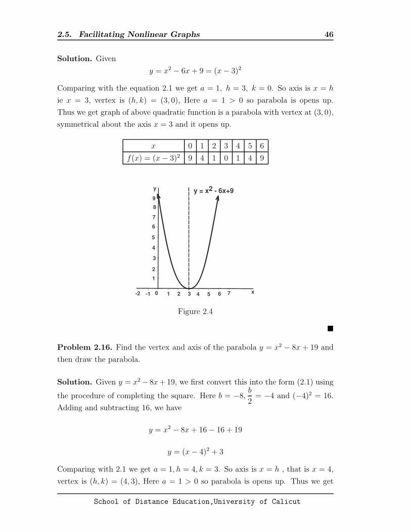
Solution. Given
y = x2 − 6x+ 9 = (x− 3)2
Comparing with the equation 2.1 we get a = 1, h = 3, k = 0. So axis is x = h
ie x = 3, vertex is (h, k) = (3, 0), Here a = 1 > 0 so parabola is opens up.
Thus we get graph of above quadratic function is a parabola with vertex at (3, 0),
symmetrical about the axis x = 3 and it opens up.
x 0 1 2 3 4 5 6
f(x) = (x− 3)2 9 4 1 0 1 4 9
0 x
y
1 2 3 4-1-2
2
4
6
5 6 7
8
y = x2 - 6x+99
7
5
3
1
Figure 2.4
�
Problem 2.16. Find the vertex and axis of the parabola y = x2 − 8x+ 19 and
then draw the parabola.
Solution. Given y = x2 − 8x+19, we first convert this into the form (2.1) using
the procedure of completing the square. Here b = −8,b
2= −4 and (−4)2 = 16.
Adding and subtracting 16, we have
y = x2 − 8x+ 16− 16 + 19
y = (x− 4)2 + 3
Comparing with 2.1 we get a = 1, h = 4, k = 3. So axis is x = h , that is x = 4,
vertex is (h, k) = (4, 3), Here a = 1 > 0 so parabola is opens up. Thus we get
School of Distance Education,University of Calicut

2.5. Facilitating Nonlinear Graphs 47
graph of above quadratic function is a parabola with vertex at (4, 3), symmetrical
about the axis x = 4 and it opens up.
x 2 3 4 5 6
f(x) = x2 − 8x+ 9 7 4 0 4 7
0 x
y
1 2 3 4-1-2
2
4
6
5 6 7
8
9
7
5
3
1
y=x2-8x+19
Figure 2.5
�
Drawing the graph of a rational function is made easier by finding the asymptotes.
The vertical asymptote is the line x = k, where k is found by setting denominator
equal to zero and solve for x. The horizontal asymptote is the line y = m, where
m is found by first solving the original equation for x, set its denominator equal
to zero and then solve for y. In Figure 2.2 as x → 0, the graph approaches the
y- axis. So y- axis is a vertical asymptote. As x → ∞, the graph approaches the
x- axis. So x- axis is a horizontal asymptote.
Problem 2.17. Draw a rough sketch of the graphs of the following rational
functions by finding (1) the vertical asymptote,(2) the horizontal asymptote, and
then (3) selecting a number of representative points on each graph to determine
its shape.
(a) y =5
x− 2
(b) y =x+ 2
x− 5
School of Distance Education,University of Calicut
2.5. Facilitating Nonlinear Graphs 48
Solution.
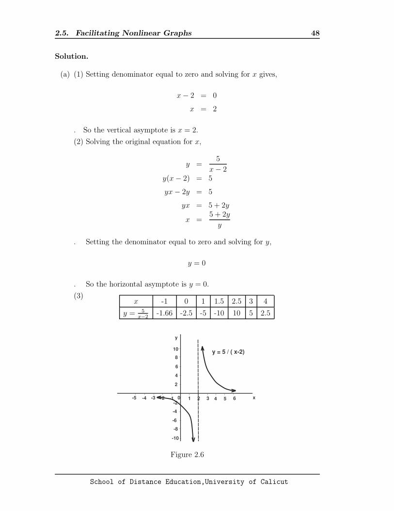
(a) (1) Setting denominator equal to zero and solving for x gives,
x− 2 = 0
x = 2
. So the vertical asymptote is x = 2.
(2) Solving the original equation for x,
y =5
x− 2y(x− 2) = 5
yx− 2y = 5
yx = 5 + 2y
x =5 + 2y
y
. Setting the denominator equal to zero and solving for y,
y = 0
. So the horizontal asymptote is y = 0.
(3)x -1 0 1 1.5 2.5 3 4
y = 5x−2
-1.66 -2.5 -5 -10 10 5 2.5
0 x
y
1 2 3 4-1-2-3-4
2
4
5 6-5-2
y = 5 / ( x-2)
6
10
8
-8
-6
-4
-10
Figure 2.6
School of Distance Education,University of Calicut

2.5. Facilitating Nonlinear Graphs 49
(b) (1) Vertical asymptote is x = 5
(2) Solving the original equation for x,
y =x+ 2
x− 5y(x− 5) = x+ 2
yx− 5y = x+ 2
yx− x = 2 + 5y
x(y − 1) = 2 + 5y
x =2 + 5y
y − 1
. Setting the denominator equal to zero and solving for y,
y − 1 = 0
y = 1
. So the horizontal asymptote is y = 1.
(3)x 1 3 4 6 7 9
y = x+2x−5
-0.75 -2.5 -6 8 4.5 2.75
0 x
y
1 2 3 4-1
-3
2
5 6
-5
-2
7
8
-6
-4
10
1
3
4
5
6
7 8 9-1-2
y= (x+2)/ (x-5)
y = 1
Figure 2.7
�
School of Distance Education,University of Calicut

2.5. Facilitating Nonlinear Graphs 50
Problem 2.18. Given the following total revenue R(x) and total cost C(x) func-
tions, express profit π as an explicit function of x and determine the maximum
level of profit by finding the vertex of π(x). Find the x-intercepts of the graph
but do not graph.
(a) R(x) = 600x− 5x2, C(x) = 100x+ 10, 500
(b) R(x) = 280x− 2x2, C(x) = 60x+ 5, 600
Solution.
(a)
π(x) = R(x)− C(x)
= 600x− 5x2 − (100x+ 10, 500)
= 600x− 5x2 − 100x− 10, 500
= −5x2 + 500x− 10, 500
= −5(x2 − 100x+ 2, 100)
Completing the square,
π(x) = −5(x2 − 100x+ 2, 100)
= −5(x2 − 100x+ (−50)2 − (−50)2 + 2, 100)
= −5((x− 50)2 − 2500 + 2100)
= −5(x− 50)2 − 400)
= −5(x− 50)2 + 2000
Comparing with (2.1) we get a = −5, h = 50, k = 2000. So vertex is
(h, k) = (50, 2000), Maximum profit π(50) = 2000.
To find x-intercepts we put π(x) = 0.
π(x) = 0
⇒ −5(x2 − 100x+ 2, 100) = 0
−5(x− 30)(x− 70) = 0
⇒ x = 30 x = 70. So x-intercepts are (30, 0), (70, 0).
School of Distance Education,University of Calicut
2.6. Exercises 51
(b)
π(x) = R(x)− C(x)
= 280x− 2x2 − (60x+ 5, 600)
= 280x− 2x2 − 60x− 5, 600
= −2x2 + 220x− 5, 600
= −2(x2 − 110x+ 2, 800)
Completing the square,
π(x) = −2(x2 − 110x+ 2, 800)
= −5(x2 − 100x+ (−55)2 − (−55)2 + 2, 800)
= −2((x− 55)2 − 3025 + 2, 800)
= −2(x− 55)2 − 225)
= −2(x− 55)2 + 450
Comparing with 2.1 we get a = −2, h = 55, k = 450. So vertex is
(h, k) = (55, 450), Maximum profit π(55) = 450.
To find x-intercepts we put π(x) = 0.
π(x) = 0
⇒ −2(x2 − 110x+ 2, 800) = 0
−2(x− 40)(x− 70) = 0
⇒ x = 40 x = 70. So x-intercepts are (40, 0), (70, 0)
�
2.6 Exercises
1. Given f(x) = 2x3 − 4x2 + 7x− 10, find f(2) and f(−3).
2. Given f(x) = x2 + 6x+ 8, find f(a) and f(a+ 3).
3. Identify the domain of the following functions:
(a)x
x2 − 36(b)
3x√8− x
School of Distance Education,University of Calicut

2.6. Exercises 52
4. Identify the range of the functions y = −5x. (1 ≤ x ≤ 4)
5. If f(x) = 6x−5 and g(x) = 8x−3, then find (f+g)(x), (f−g)(x), (f ·g)(x)and (f ÷ g)(x)
6. If f(x) = x2+6 and g(x) = 3x−7, then find (f+g)(x), (f−g)(x), (f ·g)(x)and (f ÷ g)(x)
7. If f(x) = x3, g(x) = x2 − 2x + 5 and h(x) =x
x+ 4, where (x 6= −4) find:
(a) g[f(x)] (b) f [h(x)] (c) h[f(x)] (d) h[g(x)]
8. A widow receives $5,600 a year from $50,000 placed in two bonds, one paying
10 percent and the other 12 percent. How much does she have invested in
each bond?
9. Graph the following quadratic functions and identify the vertex and axis of
each:
(a) f(x) = 5− x2
(b) f(x) = x2 + 10x+ 25
(c) f(x) = x2 + 12x+ 41
(d) f(x) = −x2 − 4x− 1
10. Draw a rough sketch of the graphs of the following rational functions by
finding (1) the vertical asymptote, (2) the horizontal asymptote, and then
(3) selecting a number of representative points on each graph to determine
its shape.
(a) y =4
x+ 3
(b) y =−2
x+ 5
(c) y =3x+ 2
4x− 6
(d) y =6x+ 1
2x− 4
School of Distance Education,University of Calicut
Chapter 3The Derivative
3.1 Limits
x → a may be read as “x tends to a ”or “x approaches a ”. This means that x
takes those values which are either less than a or greater than a but the numerical
difference between x and a can be made as small as we please.
Let f(x) be a function of x. Then f(x) is said to approach L if the difference
between f(x) and L can be made as small as possible by taking x sufficiently
near to a.That is, when x is very close to a, f(x) also becomes close to L.
we write limx→a
f(x) = L.
Assuming that limx→a
f(x) and limx→a
g(x) both exist, the rules of limits are given
below.
1. limx→a
k = k (k = a constant)
2. limx→a
xn = an (n = a positive integer)
3. limx→a
kf(x) = k limx→a
f(x) (k = a constant)
4. limx→a
[f(x)± g(x)] = limx→a
f(x)± limx→a
g(x)
5. limx→a
[f(x) · g(x)] = limx→a
f(x) · limx→a
g(x)
6. limx→a
[f(x)÷ g(x)] = limx→a
f(x)÷ limx→a
g(x), [limx→a
g(x) 6= 0]
7. limx→a
[f(x)]n = [limx→a
f(x)]n (n > 0)
53

3.1. Limits 54
Note 3.1. (a) For all polynomials f(x), limx→a
f(x) = f(a)
(b) For all rational functions f(x) = g(x)/h(x) where g(x) and h(x) are poly-
nomials and h(x) 6= 0, limx→a
f(x) = f(a)
Problem 3.1. Use the rules of limits to find the limits for the following functions
(a) limx→5
(3x2 − 6x+ 8)
(b) limx→7
[x2(x− 5)]
(c) limx→3
4x2 − 9x
x+ 7
(d) limx→2
√6x2 + 1
Solution.
(a) limx→5
(3x2 − 6x+ 8) = 3(5)2 − 6(5) + 8 = 3(25)− 30 + 8 = 75− 30 + 8 = 53
(b)
limx→7
[x2(x− 5)] = limx→7
x2 · limx→7
(x− 5)
= (7)2 · (7− 5)
= 49 · 2= 98
(c)
limx→3
4x2 − 9x
x+ 7=
limx→3
(4x2 − 9x)
limx→3
(x+ 7)
=4(3)2 − 9(3)
3 + 7
=36− 27
10
=9
10
School of Distance Education,University of Calicut

3.1. Limits 55
(d)
limx→2
√6x2 + 1 = lim
x→2(6x2 + 1)1/2
= [limx→2
(6x2 + 1)]1/2
= [6(2)2 + 1]1/2
= (25)1/2
= 5
�
Problem 3.2. Find the following limits:
(a) limx→3
x− 3
x2 − 9
(b) limx→4
x+ 4
x2 − 16
(c) limx→5
x2 − x− 20
x2 − 25
(d) limx→9
x2 + 81
x− 9
Solution.
(a) Here the limit of the denominator is zero, so rule 6. can not be used. But
we can find limit by factoring and cancelling the mutual terms.
limx→3
x− 3
x2 − 9= lim
x→3
x− 3
(x− 3)(x+ 3)= lim
x→3
1
x+ 3=
1
6
(b) Here the limit of the denominator is zero, so rule 6. can not be used. But
we can find limit by factoring and cancelling the mutual terms.
limx→4
x+ 4
x2 − 16= lim
x→4
x+ 4
(x− 4)(x+ 4)= lim
x→4
1
x− 4
The limit does not exist.
(c) Since the limit of denominator equals zero, we factor
limx→5
x2 − x− 20
x2 − 25= lim
x→5
(x− 5)(x+ 4)
(x− 5)(x+ 5)= lim
x→5
x+ 4
x+ 5=
9
10
School of Distance Education,University of Calicut

3.1. Limits 56
(d) With the limit of the denominator equal to zero, we try to factor the nu-
merator but see that it is impossible. We conclude, therefore that the limit
does not exist.
�
Note 3.2. If x takes values which are close to a and always remains on the left
of a, that is the value of x is less than a, then we say that x approaches a from
left and we write x → a−. So x → a− implies x < a.
If x takes values which are close to a and always remains on the right of a,
that is the values of x is greater than a, then we say that x approaches a from
right and we write x → a+. So x → a+ implies x > a.
Problem 3.3. Find the limits of the following functions:
(a) limx→0
1
x
(b) limx→∞
1
x
(c) limx→−∞
1
x
(d) limx→∞
2x2 − 3x
5x2 − 12
(e) limx→∞
7x3 − 5x2 + 12x
4x2 + 9x
Solution.
(a) Note that as x approaches zero from right (x → 0+), f(x) approaches
positive infinity; as x approaches zero from left (x → 0−), f(x) approaches
negative infinity. If a limit approaches either positive or negative infinity,
the limit does not exist and is written,
limx→0+
1
x= ∞ lim
x→0−
1
x= −∞
The limit does not exist.
(b) As x approaches ∞, f(x) approaches zero, so the limit exist and we write
limx→∞
1
x= 0
School of Distance Education,University of Calicut

3.1. Limits 57
(c) As x approaches −∞, f(x) approaches zero, so the limit exist and we write
limx→−∞
1
x= 0
(d) As x → ∞, both numerator and denominator become infinite. Divide
all terms by the highest power of x which appears in the function. Here
dividing all terms by x2 leaves,
limx→∞
2x2 − 3x
5x2 − 12= lim
x→∞
2− (3/x)
5− (12/x2)=
2− (0)
5− (0)=
2
5
(e) As x → ∞, both numerator and denominator become infinite. Divide
all terms by the highest power of x which appears in the function. Here
dividing all terms by x3 leaves
limx→∞
7x3 − 5x2 + 12x
4x2 + 9x= lim
x→∞
7− (5/x) + (12/x2)
(4/x) + (9/x2)=
7− 0 + 0
0 + 0
Here denominator equal to zero. So the limit does not exist.
�
Problem 3.4. Find the following limits:
(a) limx→2
6x+ 1
2x− 4
(b) limx→∞
6x+ 1
2x− 4
(c) limx→5
x+ 2
x− 5
(d) limx→∞
5
x− 2
Solution.
(a) As x → 2, the denominator approaches zero. Hence
limx→2
6x+ 1
2x− 4= ∞
School of Distance Education,University of Calicut
3.1. Limits 58
(b)
limx→∞
6x+ 1
2x− 4= lim
x→∞
6 + (1/x)
2− (4/x)=
3 + 0
4− 0=
3
4
(c) As x → 5, the denominator approaches zero. Hence
limx→5
x+ 2
x− 5= ∞
(d) As x → ∞, the denominator approaches infinity, and
limx→∞
5
x− 2= 0
�
Problem 3.5. Find the limits of the following functions involving radicals:
(a) limx→0
7√x+ 144− 2
(b) limx→36
√x− 6
x− 36
(c) limx→3
√x−
√3
x− 3
Solution.
(a) limx→0
7√x+ 144− 2
=7
12− 2=
7
10
(b) Here the limit of the denominator equal to zero. Here we multiply both
numerator and denominator by√x+ 6,
limx→36
√x− 6
x− 36= lim
x→36
√x− 6
x− 36·√x+ 6√x+ 6
= limx→36
x+ 6√x− 6
√x− 36
(x− 36)(√x+ 6)
= limx→36
(x− 36)
(x− 36)(√x+ 6)
= limx→36
1√x+ 6
=1√
36 + 6=
1
6 + 6=
1
12
∴ limx→36
√x− 6
x− 36=
1
12
School of Distance Education,University of Calicut

3.2. Continuity 59
(c) Here the limit of the denominator equal to zero. Here we multiply both
numerator and denominator by√x+
√3
limx→3
√x−
√3
x− 3= lim
x→3
√x−
√3
x− 3·√x+
√3
√x+
√3
= limx→3
x− 3
(x− 3)(√x+
√3)
= limx→3
1√x+
√3
=1√
3 +√3=
1
2√3
∴ limx→3
√x−
√3
x− 3=
1
2√3
�
3.2 Continuity
The graph of a continuous function has no break; it can be drawn without lifting
pencil from paper. A function f is continuous at x = a if all three of the following
conditions hold:
(1) f(x) is defined, that is, exists, at x = a.
(2) limx→a
f(x) exists.
(3) limx→a
f(x) = f(a).
From the properties of continuity, it can be shown that for all real x:
1. All polynomial functions are continuous.
2. All rational functions are continuous except where undefined, that is where
their denominators equal zero.
3. Suppose f(x) and g(x) are continuous at a point, at that point f(x)± g(x)
is continuous.
4. f(x) · g(x) is continuous.
School of Distance Education,University of Calicut
3.2. Continuity 60
5. f(x)÷ g(x) is continuous [g(x) 6= 0].
6. n√
f(x) is continuous [whenever n√
f(x) is defined].
Problem 3.6. Check whether the following functions are continuous at the spec-
ified points:
(a) f(x) = 14x+ 6 at x = 5
(b) f(x) =x2 + 7x+ 5
x− 2at x = 3
(c) f(x) =x− 2
x2 − 4at x = 2
Solution.
(a) (1) f(5) = 14(5) + 6 = 70 + 6 = 76 .The function is defined at x = 5.
(2) limx→5
f(x) = limx→5
(14x+ 6) = 14(5) + 6 = 76.
(3) limx→5
f(x) = 76 = f(5). So f(x) is continuous.
(b) (1) f(3) =(3)2 + 7(3) + 5
(3)− 2=
35
1= 35. The function is defined at x = 3.
(2) limx→3
f(x) = limx→3
x2 + 7x+ 5
x− 2=
(3)2 + 7(3) + 5
(3)− 2=
35
1= 35.
(3) limx→3
f(x) = 35 = f(3). So f(x) is continuous.
(c) (1)
f(2) =2− 2
(2)2 − 4
with the denominator equal to zero, f(x) is not defined at x = 2. So
f(x) is not continuous at x = 2 even though limit exist at x = 2.
(2) limx→2
f(x) = limx→2
x− 2
x2 − 4= lim
x→2
x− 2
(x− 2)(x+ 2)= lim
x→2
1
x+ 2=
1
4.
(3) limx→2
f(x) =1
46= f(2). So f(x) is discontinuous at x = 2.
�
Problem 3.7. Prove that a polynomial function is continuous for any real value
a of x, given f(x) = k0xn + k1x
n−1 + k2xn−2 + · · ·+ kn−1x+ kn
School of Distance Education,University of Calicut

3.2. Continuity 61
Solution.
(1) f(a) = k0an + k1a
n−1 + k2an−2 + · · ·+ kn−1a+ kn.
(2)
limx→a
f(x) = limx→a
(k0xn + k1x
n−1 + k2xn−2 + · · ·+ kn−1x+ kn)
= limx→a
k0xn + lim
x→ak1x
n−1 + · · ·+ limx→a
kn−1x+ limx→a
kn
= k0 limx→a
xn + k1 limx→a
xn−1 + · · ·+ kn−1 limx→a
x+ limx→a
kn
= k0an + k1a
n−1 + k2an−2 + · · ·+ kn−1a + kn.
(3) limx→a
f(x) = f(a). So the polynomial is continuous at x = a.
�
Problem 3.8. For the following functions find the points of discontinuity:
(a) f(x) = 7x2 − 4x+ 23
(b) g(x) =13x
(x+ 2)(x− 4)
(c) h(x) =x+ 7
x2 − 49
(d) f(x) =√14− x
Solution.
(a) Since f(x) = 7x2 − 4x + 23 is a polynomial it is continuous for all real
values of x. So there is no point of discontinuity.
(b) Note that g(x) =13x
(x+ 2)(x− 4)is not defined for any value of x which
would make the denominator equal to zero. Here denominator becomes
zero when x takes values −2 and 4. So points of discontinuities are x = −2
and x = 4
(c) h(x) =x+ 7
x2 − 49=
x+ 7
(x+ 7)(x− 7)=
1
x− 7.
Note that even though h(x) can be reduced to1
x− 7, if x = −7, the denom-
inator of the original function is zero and h(x) is undefined. Hence h(x) is
discontinuous at both 7 and -7.
School of Distance Education,University of Calicut

3.3. The Slope of a Curvilinear Function 62
(d) Since a square root is defined only for non negative numbers, f(x) is not
defined for x > 14. So points of discontinuities are x > 14.
�
3.3 The Slope of a Curvilinear Function
Linear functions are easy to use because the rate of change in the dependent
variable as the independent variable changes is constant. For many relations,
however, the rate of change in y as x changes is not constant. Functions for
which the rate of change, or slope, varies are called curvilinear functions. As
the name suggests, the graph of a curvilinear function is a curve rather than a
straight line.
The slope of a curve varies continuously with movements along the curve.
Geometrically, the slope of a curvilinear function at a given point is measured by
the slope of a line drawn tangent (a tangent line to a circle is a straight line that
touches the circle at only one point) to the function at that point.
x
y Tangent Line T
Secant Line S
y2= f(x1+ x)
y1=f(x1)
xx2=x1+x1 x
y
Figure 3.1
A secant line S is a straight line that intersects the graph of a function at two
points. From above Figure
Slope S =y2 − y1x2 − x1
School of Distance Education,University of Calicut

3.3. The Slope of a Curvilinear Function 63
By letting x2 = x1 + ∆x and y2 = f(x1 + ∆x), the slope of the secant line can
also be expressed by
Slope S =f(x1 +∆x)− f(x1)
(x1 +∆x)− x1
=f(x1 +∆x)− f(x1)
∆x
If the distance between x2 and x1 is made smaller and smaller, that is if
∆x → 0, the secant line draws closer and closer to the tangent line. If the slope
of the secant line approaches a limit as ∆x → 0, the limit is the slope of the
tangent line T , hence the slope of the function itself at the point, and is written
Slope T = lim∆x→0
f(x1 +∆x)− f(x1)
∆x(3.1)
In many texts h is used in place of ∆x, giving,
Slope T = limh→0
f(x1 + h)− f(x1)
h(3.2)
Problem 3.9. For the following functions find (1) The slope (2) The equation
of the tangent line at the given point:
(a) y = x2 − 2 at (3, 7)
(b) y = 2x2 − 3 at (2, 5)
(c) y =1
xat (1, 1)
Solution.
(a) (1) Using (3.1) for the formula for the slope of a tangent line to find the
slope S of the curve at the given point:
Slope S = lim∆x→0
f(x+∆x)− f(x)
∆x
Substituting x2 − 2 for f(x),
Slope S = lim∆x→0
[(x+∆x)2 − 2]− (x2 − 2)
∆x
School of Distance Education,University of Calicut
3.3. The Slope of a Curvilinear Function 64
Simplifying above equation we get,
Slope S = lim∆x→0
(x2 + 2x∆x+ (∆x)2 − 2)− (x2 − 2)
∆x
= lim∆x→0
(x2 + 2x∆x+ (∆x)2 − 2− x2 + 2)
∆x
= lim∆x→0
2x∆x+ (∆x)2
∆x
= lim∆x→0
2x+∆x
= 2x
So Slope S = 2x.
(2) At x = 3, S = 2(3) = 6, which is the slope of the function at (3, 7).
Substituting m = 6 in point-slope formula y − y1 = m(x− x1) we get,
y − 7 = 6(x− 3)
y − 7 = 6x− 18
y = 6x− 18 + 7
y = 6x− 11
So equation of tangent line at (3, 7) is y = 6x− 11.
(b) (1)
Slope S = lim∆x→0
f(x+∆x)− f(x)
∆x
Substituting 2x2 − 3 for f(x),
Slope S = lim∆x→0
[2(x+∆x)2 − 3]− (2x2 − 3)
∆x
Simplifying above equation we get,
Slope S = lim∆x→0
2(x2 + 2x∆x+ (∆x)2)− 3− (2x2 − 3)
∆x
School of Distance Education,University of Calicut
3.3. The Slope of a Curvilinear Function 65
= lim∆x→0
2x2 + 4x∆x+ 2(∆x)2 − 3− 2x2 + 3)
∆x
= lim∆x→0
4x∆x+ 2(∆x)2
∆x
= lim∆x→0
4x+ 2∆x
= 4x
So Slope S = 4x.
(2) At x = 2, S = 4(2) = 8, which is the slope of the function at (2, 5).
Substituting m = 8 in point-slope formula y − y1 = m(x− x1) we get,
y − 5 = 8(x− 2)
y − 5 = 8x− 16
y = 8x− 16 + 5
y = 8x− 11
So equation of tangent line at (2, 5) is y = 8x− 11.
(c)
Slope S = lim∆x→0
f(x+∆x)− f(x)
∆x
Substituting1
xfor f(x),
Slope S = lim∆x→0
1
x+∆x− 1
x∆x
Simplifying above equation we get,
Slope S = lim∆x→0
x− (x+∆x)
(x+∆x)x
∆x
= lim∆x→0
x− (x+∆x)
(x+∆x)x∆x
School of Distance Education,University of Calicut

3.4. Rates of Change 66
= lim∆x→0
x− x−∆x
(x+∆x)x∆x
= lim∆x→0
−∆x
(x+∆x)x∆x
= lim∆x→0
−1
(x+∆x)x
= lim∆x→0
−1
x2 + x∆x
=−1
x2
So Slope S =−1
x2
(2) At x = 1, S =−1
(1)2= −1, which is the slope of the function at (1, 1).
Substituting m = −1 in point-slope formula y − y1 = m(x− x1) we get,
y − 1 = −1(x− 1)
y − 1 = −x+ 1
y = −x+ 1 + 1
y = −x+ 2
So equation of tangent line at (1, 1) is, y = −x+ 2.
�
3.4 Rates of Change
Given a function y = f(x), the average rate of change from x1 to x2 is defined as
the change in the dependent variable divided by the change in the independent
variable:
Average rate of change =∆y
∆x=
y2 − y1x2 − x1
=f(x2)− f(x1)
x2 − x1
Average rate =f(x1 +∆x)− f(x1)
∆x(3.3)
School of Distance Education,University of Calicut

3.4. Rates of Change 67
As ∆x → 0, assuming the limit exists, the average rate of change approaches the
instantaneous rate of change, which is defined by
Instantaneous rate = lim∆x→0
f(x1 +∆x)− f(x1)
∆x(3.4)
Problem 3.10. The laws of physics indicate that a lead pellet dropped from a
bridge will fall a distance of y feet in t seconds, given by the formula y = f(t) =
16t2, with velocity = distance divided by time, Estimate (a) The average velocity
(AV) of the pellet between t = 3 and t = 4, (b) The average velocity for a small
change in time ∆t starting with t = 3 and (c) The instantaneous velocity at t = 3.
Solution.
(a) Average velocity =∆y
∆x=
y2 − y1x2 − x1
=f(4)− f(3)
4− 3
. =16(4)2 − 16(3)2
1=
256− 144
1= 112
So average velocity of the pellet between t = 3 and t = 4 is 112 ft/sec.
(b) Average velocity for a small change in time, ∆t, using (3.3) and starting
from t = 3
Average velocity =f(3 + ∆t)− f(3)
(3 + ∆t)− 3
=16(3 + ∆t)2 − 16(3)2
∆t
=16[9 + 6∆t+ (∆t)2]− 16(9)
∆t
=144 + 96∆t + 16(∆t)2 − 144
∆t
=96∆t+ 16(∆t)2
∆t
=∆t(96 + 16(∆t))
∆t
= 96 + 16∆t ft/sec
If at t = 3, ∆t = 1, AV= 96 + 16(1) = 112 ft/sec ;
School of Distance Education,University of Calicut
3.4. Rates of Change 68
if ∆t = 14, AV = 96 + 16(1
4) = 100 ft/sec.
(c) If ∆t → 0, assuming the limit exist, we have from (3.4) the instantaneous
velocity,
Instantaneous velocity at t = 3 = lim∆t→0
16(3 + ∆t)2 − 16(3)2
∆t
= lim∆t→0
(96 + 16∆t)
= 96 ft/sec
�
Problem 3.11. A trunk travels a distance of w miles in t hours given by the
function w(t) = 10t2 + 5t. Estimate (a) The average velocity (AV) of the pellet
between t = 2 and t = 3 , (b) The average velocity for a small change in time ∆t
starting with t = 2 and (c) The instantaneous velocity at t = 2.
Solution.
(a)
AV =w(3)− w(2)
3− 2
=[10(3)2 + 5(3)]− [10(2)2 + 5(2)]
3− 2
=[10(9) + 15]− [10(4) + 10]
1
=(90 + 15)− (40 + 10)
1
=(105− 50
1= 55 mph
(b) Starting at t = 2,
AV =w(2 + ∆t)− w(2)
(2 + ∆t)− 2
School of Distance Education,University of Calicut

3.4. Rates of Change 69
=[10(2 + ∆t)2 + 5(2 + ∆t)]− [10(2)2 + 5(2)]
∆t
=[10(4 + 4∆t + (∆t)2) + 10 + 5∆t]− [10(4) + 10]
∆t
=[40 + 40∆t+ 10(∆t)2 + 10 + 5∆t]− [40 + 10]
∆t
=[50 + 45∆t+ 10(∆t)2]− [50]
∆t
=50 + 45∆t + 10(∆t)2 − 50
∆t
=45∆t+ 10(∆t)2
∆t
= 45 + 10∆t
If at t = 2, ∆t = 1, AV= 45 + 10(1) = 55 mph; if ∆t = 0.5, AV =
45 + 10(0.5) = 45 + 5 = 50 mph.
(c) If ∆t → 0, assuming the limit exist, we have from (3.4) the instantaneous
velocity(IV)
IV at t = 2 = lim∆t→0
[10(2 + ∆t)2 + 5(2 + ∆t)]− [10(2)2 + 5(2)]
∆t
= lim∆t→0
(45 + 10∆t)
= 45 mph at t = 2
�
School of Distance Education,University of Calicut

3.5. The Derivative 70
3.5 The Derivative
Given a function y = f(x), the derivative of the function f at x, written f ′(x) ordy
dxis defined as
f ′(x) = lim∆x→0
f(x+∆x)− f(x)
∆x(3.5)
provided the limit exists.
We read f ′(x) as “the derivative of f with repect to x ”, or “f prime of x”.
The derivative of a function, f ′(x) of simply f ′, is itself a function which
measures the slope and the instantaneous rate of change of the original function
f(x) at a given point. The process of finding a derivative is called differentiation.
Problem 3.12. For each of the following functions use delta process to (1) find
the derivative and then (2) Evaluate the derivative for the given value of x :
(a) f(x) = 5x+ 7 at x = 8
(b) f(x) = x2 − 6 at x = −5
(c) f(x) =1
3x+ 7at x = −2
(d) f(x) =√x at x = 16
Solution.
(a) (1)
f ′(x) = lim∆x→0
f(x+∆x)− f(x)
∆x
Substituting 5x+ 7 for f(x),
f ′(x) = lim∆x→0
[5(x+∆x) + 7]− (5x+ 7)
∆x
= lim∆x→0
[5x+ 5∆x+ 7− (5x+ 7)
∆x
School of Distance Education,University of Calicut
3.5. The Derivative 71
= lim∆x→0
(5x+ 5∆x+ 7− 5x− 7)
∆x
= lim∆x→0
5∆x
∆x
= lim∆x→0
5 = 5
So f ′(x) = 5.
(2) Derivative at x = 8 is f ′(8) = 5.
(b) (1)
f ′(x) = lim∆x→0
f(x+∆x)− f(x)
∆x
Substituting x2 − 6 for f(x),
f ′(x) = lim∆x→0
[(x+∆x)2 − 6]− (x2 − 6)
∆x
= lim∆x→0
[x2 + 2x∆x + (∆x)2 − 6]− (x2 − 6)
∆x
= lim∆x→0
x2 + 2x∆x+ (∆x)2 − 6− x2 + 6
∆x
= lim∆x→0
2x∆x+ (∆x)2
∆x
= lim∆x→0
2x+∆x
= 2x
So f ′(x) = 2x.
(2) Derivative at x = −5 is f ′(−5) = −10.
(c) (1)
f ′(x) = lim∆x→0
f(x+∆x)− f(x)
∆x
School of Distance Education,University of Calicut

3.5. The Derivative 72
Substituting1
3x+ 7for f(x),
f ′(x) = lim∆x→0
1
3(x+∆x) + 7− 1
3x+ 7
∆x
= lim∆x→0
(3x+ 7)− (3x+ 3∆x+ 7)
(3x+ 3∆x+ 7)(3x+ 7)
∆x
= lim∆x→0
1
∆x
[
(3x+ 7)− (3x+ 3∆x+ 7)
(3x+ 3∆x+ 7)(3x+ 7)
]
= lim∆x→0
1
∆x
[
3x+ 7− 3x− 3∆x− 7
(9x2 + 21x+ 9x∆x+ 21∆x+ 21x+ 49)
]
= lim∆x→0
1
∆x
[ −3∆x
(9x2 + 42x+ 49) + 9x∆x+ 21∆x
]
= lim∆x→0
1
∆x
[ −3∆x
(3x+ 7)2 + 9x∆x+ 21∆x
]
= lim∆x→0
−3
(3x+ 7)2 + 9x∆x+ 21∆x
=−3
(3x+ 7)2
So f ′(x) =−3
(3x+ 7)2.
(2) Derivative at x = −2 is f ′(−2) =−3
[(3(−2) + 7)]2=
−3
(−6 + 7)2= −3.
(d) (1)
f ′(x) = lim∆x→0
f(x+∆x)− f(x)
∆x= lim
∆x→0
√x+∆x−√
x
∆x
Denominator approaches zero as ∆x → 0, So we rationalize the numerator
f ′(x) = lim∆x→0
√x+∆x−√
x
∆x·√x+∆x+
√x√
x+∆x+√x
School of Distance Education,University of Calicut
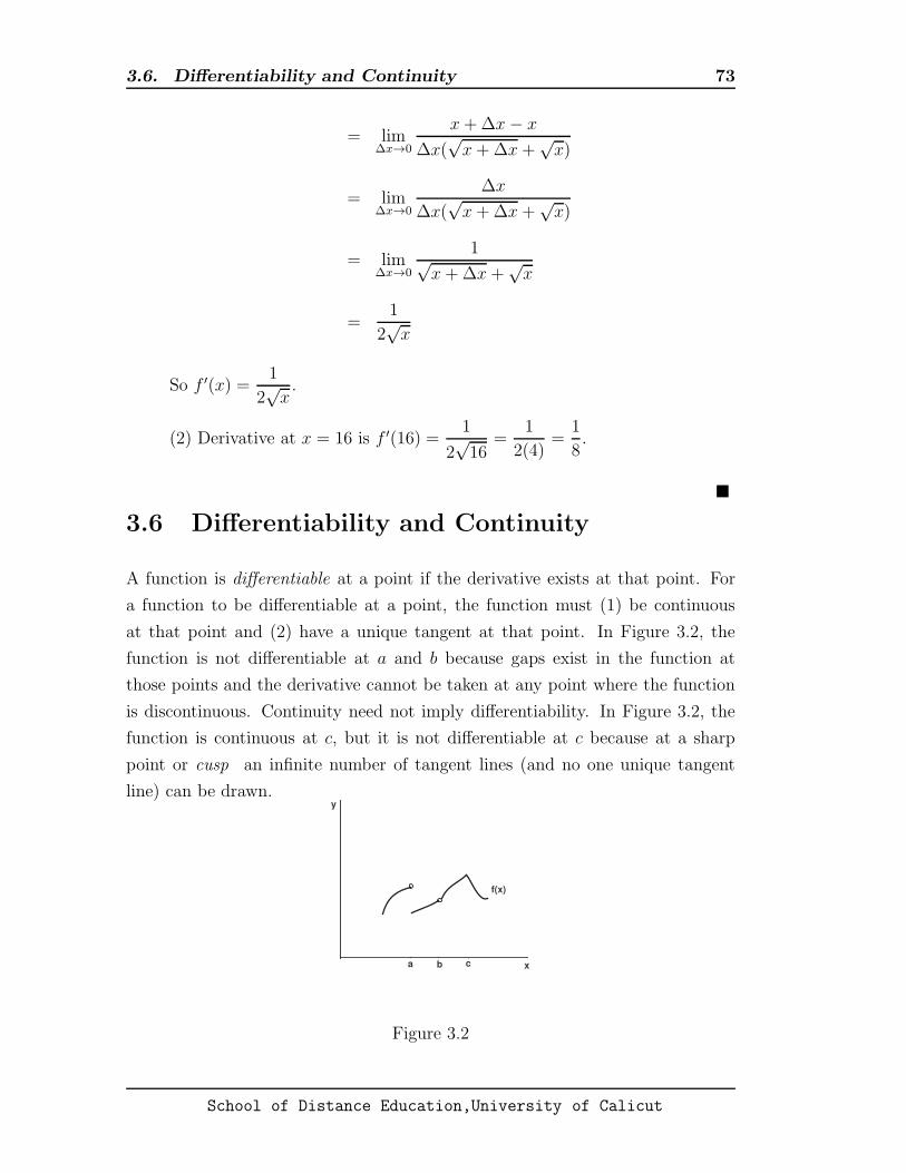
3.6. Differentiability and Continuity 73
= lim∆x→0
x+∆x− x
∆x(√x+∆x+
√x)
= lim∆x→0
∆x
∆x(√x+∆x+
√x)
= lim∆x→0
1√x+∆x+
√x
=1
2√x
So f ′(x) =1
2√x.
(2) Derivative at x = 16 is f ′(16) =1
2√16
=1
2(4)=
1
8.
�
3.6 Differentiability and Continuity
A function is differentiable at a point if the derivative exists at that point. For
a function to be differentiable at a point, the function must (1) be continuous
at that point and (2) have a unique tangent at that point. In Figure 3.2, the
function is not differentiable at a and b because gaps exist in the function at
those points and the derivative cannot be taken at any point where the function
is discontinuous. Continuity need not imply differentiability. In Figure 3.2, the
function is continuous at c, but it is not differentiable at c because at a sharp
point or cusp an infinite number of tangent lines (and no one unique tangent
line) can be drawn.
x
y
a cb
f(x)
Figure 3.2
School of Distance Education,University of Calicut

3.7. Applications for the Social Sciences, Business, and Economics74
3.7 Applications for the Social Sciences, Busi-
ness, and Economics
Economists are particularly interested inmarginal rates of change, such as marginal
cost, marginal revenue, marginal utility, marginal product, etc., all of which are
measured mathematically by derivative.
Marginal cost is defined as the change in total cost associated with a small
change in the quantity produced. It is measured by the derivative of the total
cost function. If C(x) is the total cost function, then C ′(x) is the marginal
cost function. Similarly, if R(x) is the total revenue function, then R′(x) is the
marginal revenue function.
Problem 3.13. Given the total cost function C (in dollars) of producing x
pounds of fertilizer, C(x) = 0.5x2 + 1.5x+ 8, Find
(a) The average cost (AC) of production between x = 4 and x = 6.
(b) The AC of production for a small increase starting at x = 4.
(c) The marginal cost (MC) at x = 4.
Solution.
(a)
AC =C(6)− C(4)
6− 4
=[0.5(6)2 + 1.5(6) + 8]− [0.5(4)2 + 1.5(4) + 8]
2
=[0.5(36) + 9 + 8]− [0.5(16) + 6 + 8]
2
=(18 + 9 + 8)− (8 + 6 + 8)
2
=35− 22
2
=13
2= 6.5
School of Distance Education,University of Calicut

3.7. Applications for the Social Sciences, Business, and Economics75
(b)
AC =C(x+∆x)− C(x)
∆x
=[0.5(x+∆x)2 + 1.5(x+∆x) + 8]− [0.5x2 + 1.5x+ 8]
∆x
=[0.5(x2 + 2x∆x+ (∆x)2) + 1.5x+ 1.5∆x+ 8]− [0.5x2 + 1.5x+ 8]
∆x
=[0.5x2 + x∆x + 0.5(∆x)2 + 1.5x+ 1.5∆x+ 8]− [0.5x2 + 1.5x+ 8]
∆x
=0.5x2 + x∆x+ 0.5(∆x)2 + 1.5x+ 1.5∆x+ 8− 0.5x2 − 1.5x− 8
∆x
=x∆x + 0.5(∆x)2 + 1.5∆x
∆x
= x+ 0.5∆x+ 1.5
= x+ 1.5 + 0.5∆x
If at x = 4, ∆x = 1, AC = 4 + 1.5 + 0.5(1) = 6; ∆x = 2, AC = 4 + 1.5 +
0.5(2) = 6.5.
(c) Marginal cost MC= lim∆x→0
C(x+∆x)− C(x)
∆x
MC = lim∆x→0
[0.5(x+∆x)2 + 1.5(x+∆x) + 8]− [0.5x2 + 1.5x+ 8]
∆x
= lim∆x→0
(x+ 1.5 + 0.5∆x)
= x+ 1.5
At x = 4, MC = (4) + 1.5 = 5.5.
�
School of Distance Education,University of Calicut

3.7. Applications for the Social Sciences, Business, and Economics76
Problem 3.14. Given the total revenue function R from the sale of x units,
R(x) = 150x− 3x2, Find
(a) The average revenue (AR) of sales between x = 15 and x = 20.
(b) The AR of sales for a small increase of sales starting at x = 15.
(c) The marginal cost (MR) at x = 15.
Solution.
(a)
AR =R(20)−R(15)
20− 15
=[150(20)− 3(20)2]− [150(15)− 3(15)2]
5
=[3000− 3(400)]− [2250− 3(225)]
5
=(3000− 1200)− (2250− 675)
5
=1800− 1575
5
=225
5= 45
(b)
AR =R(x+∆x)− R(x)
∆x
=[150(x+∆x)− 3(x+∆x)2]− [150x− 3x2]
∆x
=[150x+ 150∆x− 3(x2 + 2x∆x+ (∆x)2)]− [150x− 3x2]
∆x
=[150x+ 150∆x− 3x2 − 6x∆x− 3(∆x)2]− [150x− 3x2]
∆x
School of Distance Education,University of Calicut
3.8. Exercises 77
=[150x+ 150∆x− 3x2 − 6x∆x− 3(∆x)2 − 150x+ 3x2]
∆x
=150∆x− 6x∆x− 3(∆x)2
∆x
=∆x(150− 6x− 3∆x)
∆x
= 150− 6x− 3∆x
If at x = 15, ∆x = 5, AR = 150− 6(15)− 3(5) = 150− 90− 15 = 45.
(c) Marginal revenue MR =dR
dx= lim
∆x→0
R(x+∆x)−R(x)
∆x
MR =[150(x+∆x)− 3(x+∆x)2]− [150x− 3x2]
∆x
= lim∆x→0
(150− 6x− 3∆x)
= 150− 6x
At x = 15, MR = 150− 6(15) = 150− 90 = 60.
�
3.8 Exercises
1. Use the rules of limits to find the limits for the following functions:
(a) limx→−4
(2x2 + 5x− 22)
(b) limx→3
(5x2 − 13)1/3
(c) limx→−4
5x2 − 9x+ 22
2x2 + 7
2. Find the following limits:
(a) limx→−3
x− 3
x2 − 9
School of Distance Education,University of Calicut

3.8. Exercises 78
(b) limx→−4
4 + x
16− x2
(c) limx→3
x2 − x− 6
x− 3
3. Find the following limits:
(a) limx→∞
x− 11
3x2 + 5x+ 9
(b) limx→∞
8x3 − 5x2 + 13x
2x3 + 7x2 − 18x
4. Find the limits of the following functions involving radicals:
(a) limx→0
4
23−√x+ 49
(b) limx→16
√x− 4
x− 16
(c) limx→9
√x−
√9
x− 9
(d) limx→0
√x+ 25− 5
x
5. For the following functions find the points of discontinuities:
(a) g(x) =6x
x− 5
(b) f(x) =x+ 6
x2 + 2x− 24
(c) h(x) =√x− 22
6. Find the slope of the function y = x2 + 10x+ 25 , also find the equation of
the tangent line at the point (−3, 4)
7. A particle moved by an accelerator a distance w miles in t seconds given by
the function w(t) = 25t2 +45t. Find (a) the average velocity between t = 1
and t = 3, (b) the average velocity for a small change in time starting at
t = 1, and (c) the instantaneous velocity at t = 1.
8. Given the supply curve S(p) = 50x2, find (a) the average change in supply
AS from p = $3 to p = $5, (b) the average change in supply for a small
change in price at p = 3, and (c) the instantaneous change in supply IS at
p = 3.
School of Distance Education,University of Calicut
Chapter 4Differentiation
4.1 Derivative Notation
The derivative of a function can be expressed in several different ways. If y =
f(x), the derivative can be expressed as
f ′(x) y′dy
dx
df
dx
d
dx[f(x)] or Dx[f(x)]
If y = φ(t), the derivative can be written as
φ′(t) y′dy
dt
dφ
dt
d
dt[φ(t)] or Dt[φ(t)]
If the derivative of y = f(x) is evaluated at x = a, proper notation includes f ′(a)
anddy
dx
∣
∣
∣
∣
a
.
Example 4.1. If y = 2x3 + 4x+ 6, the derivative can be written as
y′dy
dx
d
dx[2x2 + 4x+ 6] or Dx[2x
2 + 4x+ 6]
4.2 Rules of Differentiation
The process of finding the derivative of a function is known as differentiation
The Constant Function Rule
The derivative of a constant function f(x) = k, where k is a constant, is zero.
Example 4.2. If f(x) = 5 then f ′(x) = 0 ; If f(x) = 8 then f ′(x) = 0
79

4.2. Rules of Differentiation 80
The Linear Function Rule
The derivative of a linear function f(x) = mx + b, is equal to m, the coefficient
of x.
Example 4.3. If f(x) = 2x+ 3 then f ′(x) = 2
If f(x) = −5x+ 12 then f ′(x) = −5
If f(x) = 14x+ 7 then f ′(x) = 1
4
The Power Function Rule
The derivative of a power function f(x) = xn, where n is any real number, is
equal to nxn−1
Example 4.4.
If f(x) = x3, f ′(x) = 3x3−1 = 3x2
If f(x) = x5, f ′(x) = 5x5−1 = 5x4
If f(x) = x3
2 , f ′(x) =3
2x
3
2−1 =
3
2x
1
2
The Rule for Constant Times a Function
If f(x) = kg(x), where k is a real number and g(x) is a differentiable function
then f ′(x) = kg′(x)
Example 4.5.
If f(x) = 4x3, f ′(x) = 4(3x3−1) = 12x2
If f(x) = −7x5, f ′(x) = −7(5x5−1) = −35x4
The Rule for Sum and Differences
Let f(x) = g(x) + h(x) where g(x) and h(x) are both differentiable functions.
Then f ′(x) = g′(x) + h′(x), Similarly if f(x) = g(x)− h(x), then f ′(x) = g′(x)−h′(x).
Example 4.6.
If f(x) = 8x4 + 4x3, f ′(x) = 8(4x4−1) + 4(3x3−1) = 32x3 + 12x2
If f(x) = 3x6 − 7x5 − 2, f ′(x) = 3(6x6−1)− 7(5x5−1)− 0 = 18x5 − 35x4
School of Distance Education,University of Calicut
4.2. Rules of Differentiation 81
Problem 4.1. Differentiate each of the following functions. Use the different
notations:
(a) f(x) = 13 (b) y = 7x− 2 (c) y = 7x4 (d) y = 4x−3
(e) f(x) = 25√x
Solution.
(a) f(x) = 13 ⇒ f ′(x) = 0 (Constant Rule)
(b) y = 7x− 2 ⇒ dy
dx= 7 (Linear Function Rule)
(c) y = 7x4 ⇒ y′ = 7(4x4−1) = 7(4x3) = −28x3 (Power Function Rule)
(d) y = 4x−3 ⇒ y′ = 4(−3x−3−1) = −12x−4 =−12
x4(Power Function Rule)
(e) f(x) = 25√x,⇒ Dx(25
√x) = Dx(25x
1
2 )
. = 25(12x[(1/2)−1]) = 12.5x−1/2 =
12.5√x
(Power Function Rule)
�
Problem 4.2. Use the rule for sums and differences to differentiate the following
functions, treating the variable on the left as dependent variable and right as
independent variable.
(a) R = 6t2 + 11t− 9
(b) p = 7q5 − 9q3
(c) u =1
x2− 6
x3= x−2 − 6x−3
Solution.
(a)dR
dt= 12t+ 11
(b)dp
dq= 35q4 − 27q2
(c) u′ = −2x−3 − 6(−3x−4) = −2x−3 + 18x−4 =−2
x3+
18
x4
�
School of Distance Education,University of Calicut

4.2. Rules of Differentiation 82
The Product Rule
If f(x) = g(x) · h(x), where g(x) and h(x) are both differentiable function then,
f ′(x) = g(x) · h′(x) + h(x) · g′(x) (4.1)
Problem 4.3. Differentiate following functions using product rule:
(a) y = 8x3(5x− 2)
(b) y = x2(x− 1)
(c) y = (6x2 − 7)(3x4)
(d) f(x) = (5x3 + 8x2)(4x5 − 2)
Solution.
(a) We have if f(x) = g(x) · h(x) then f ′(x) = g(x) · h′(x) + h(x) · g′(x)Let g(x) = 8x3 and h(x) = 5x − 2. Then g′(x) = 24x2 and h′(x) = 5.
Substituting these values in the product rule formula,
y′ = 8x3(5) + (5x− 2)24x2 = 40x3 + 120x3 − 48x2 = 160x3 − 48x2
(b) y′ = x2(1) + (x− 1)(2x) = x2 + 2x2 − 2x = 3x2 − 2x
(c)
y′ = (6x2 − 7)(12x3) + 3x4(12x)
= 72x5 − 84x3 + 36x5
= 108x5 − 84x3
(d)
f ′(x) = (5x3 + 8x2)(20x4) + (4x5 − 2)(15x2 + 16x)
= (100x7 + 160x6) + (60x7 + 64x6 − 30x2 − 32x)
= 160x7 + 224x6 − 30x2 − 32x
�
School of Distance Education,University of Calicut

4.2. Rules of Differentiation 83
The Quotient Rule
If f(x) =g(x)
h(x), where g(x) and h(x) are both differentiable function and h(x) 6= 0
then,
f ′(x) =h(x) · g′(x)− g(x) · h′(x)
[h(x)]2(4.2)
Problem 4.4. Differentiate following functions using quotient rule:
(a) f(x) =2x4
5x− 6
(b) y =7x3
4x+ 9
(c) y =4x3 − 11
3x2 + 7
Solution.
(a) We have If f(x) =g(x)
h(x)(h(x) 6= 0) then
f ′(x) =h(x) · g′(x)− g(x) · h′(x)
[h(x)]2
Let g(x) = 2x4 and h(x) = 5x − 6; then g′(x) = 8x3 and h′(x) = 5.
Substituting these values in the quotient rule formula,
f ′(x) =(5x− 6)(8x3)− 2x4(5)
(5x− 6)2
=(40x4 − 48x3)− 10x4
(5x− 6)2
=40x4 − 48x3 − 10x4
(5x− 6)2
=30x4 − 48x3
(5x− 6)2
(b) Let g(x) = 7x3 and h(x) = 4x + 9; then g′(x) = 21x2 and h′(x) = 4.
Substituting these values in the quotient rule formula,
School of Distance Education,University of Calicut

4.2. Rules of Differentiation 84
y′ =(4x+ 9)(21x2)− 7x3(4)
(4x+ 9)2
=(84x3 + 189x2)− 28x3
(4x+ 9)2
=84x3 + 189x2 − 28x3
(4x+ 9)2
=56x3 + 189x2
(4x+ 9)2
(c)
dy
dx=
(3x2 + 7)(12x2)− (4x3 − 11)(6x)
(3x2 + 7)2
=(36x4 + 84x2)− (24x4 − 66x)
(3x2 + 7)2
=36x4 + 84x2 − 24x4 + 66x
(3x2 + 7)2
=12x4 + 84x2 + 66x
(3x2 + 7)2
�
The Generalized Power Function Rule
If f(x) = [g(x)]n, where g(x) is a differentiable function and n is any real number
then,
f ′(x) = n[g(x)]n−1 · g′(x) (4.3)
Problem 4.5. Given y = (4x + 9)2, (a) find the derivative directly, using the
generalized power function rule. (b) Simplify the function first by squaring it and
then take the derivative. (c) Compare the results.
Solution.
(a) Let g(x) = 4x + 9, g′(x) = 4, and n = 2. Substitute these values in the
generalized power function rule,
y′ = 2(4x+ 9)2−1 · 4 = 8(4x+ 9) = 32x+ 72
School of Distance Education,University of Calicut

4.2. Rules of Differentiation 85
(b) Square the function first and then take the derivative,
y = (4x+ 9)2
y = 16x2 + 72x+ 81
y′ = 32x+ 72
(c) The derivatives are identical but the generalized power function rule is faster
and more practical for higher, negative, and fractional values of n.
�
Problem 4.6. Differentiate following functions using the generalized power func-
tion rule:
(a) f(x) = (2x3 + 7)5
(b) y =√16− x2
Solution.
(a) Here g(x) = 2x3 + 7, g′(x) = 6x2 and n = 5. Substitute these values in the
generalized power function rule,
y′ = 5(2x3 + 7)5−1 · 6x2 = 5(2x3 + 7)4 · 6x2 = 30x2(2x3 + 7)4
(b) Convert the radical to a power function, then differentiate,
y = (16− x2)1/2
y′ =1
2(16− x2)−1/2 · (−2x)
= −x(16− x2)−1/2
=−x√16− x2
�
School of Distance Education,University of Calicut

4.2. Rules of Differentiation 86
The Chain Rule
If f(x) = g[h(x)], where g(x) and h(x) are both differentiable functions then
f ′(x) = g′[h(x)] · h′(x) (4.4)
The chain rule is also called the composite function rule or the function of a
function rule
Problem 4.7. Find the derivative of the following function using chain rule
(a) f(x) =√8x+ 9
(b) f(x) = (12x+ 9)4
(c) f(x) = 2(4x2 + 9)3
Solution.
(a) Let g(x) =√x and h(x) = 8x+ 9, then g′(x) =
1
2x−1/2, h′(x) = 8.
Note that f(x) =√8x+ 9 =
√
h(x) = g[h(x)]
Substituting h(x) for x in g′(x),
g′[h(x)] = g′[(8x+ 9)] =1
2(8x+ 9)−1/2
Using chain rule we get,
f ′(x) =1
2(8x+ 9)−1/2 · 8 = 4(8x+ 9)−1/2 =
4√8x+ 9
(b) Let g(x) = x4 and h(x) = 12x+ 9, then g′(x) = 4x3 , h′(x) = 12
Note that f(x) = (12x+ 9)4 = (h(x))4 = g[h(x)]
Substituting h(x) for x in g′(x),
g′[h(x)] = g′[(12x+ 9)] = 4(12x+ 9)3.
Using chain rule we get,
f ′(x) = 4(12x+ 9)3 · 12 = 48(12x+ 9)3
School of Distance Education,University of Calicut

4.2. Rules of Differentiation 87
(c) Let g(x) = 2x3 and h(x) = 4x2 + 9, then g′(x) = 6x2 , h′(x) = 8x
Note that f(x) = 2(4x2 + 9)3 = 2(h(x))3 = g[h(x).
Substituting h(x) for x in g′(x),
g′[h(x)] = g′[(4x2 + 9)] = 6(4x2 + 9)2.
Using chain rule we get,
f ′(x) = 6(4x2 + 9)2 · 8x = 48x(4x2 + 9)2
�
The chain rule is also expressed in the following notation. If y is a function of u
and u is a function of x, that is y = f(u) and u = g(x), then the derivative of y
with respect to x is given by the chain rule as
dy
dx=
dy
du· dudx
Problem 4.8. Differentiate the following functions:
(a) y = (13x− 4)6
(b) y = (x2 + 5)3
Solution.
(a) Let y = u6 and u = 13x− 4, then
dy
du= 6u5,
du
dx= 13
Substitute in the chain rule
dy
dx=
dy
du· dudx
we get,dy
dx= 6u5 · 13 = 78u5
Then replace u with 13x− 4 we get,
dy
dx= 78(13x− 4)5
School of Distance Education,University of Calicut

4.3. Higher Order Derivatives 88
(b) Let y = u3 and u = x2 + 5, then
dy
du= 3u2,
du
dx= 2x
Substitute in the chain rule
dy
dx=
dy
du· dudx
we get,dy
dx= 3u2 · 2x = 6xu2
Then replace u with x2 + 5 we get,
dy
dx= 6x(x2 + 5)2
�
4.3 Higher Order Derivatives
The second-order derivative, written f ′′(x), measures the slope and rate of change
of the first derivative. The third-order derivative, written [f ′′′(x)], measures the
slope and rate of change of the second-order derivative, etc. Higher-order deriva-
tives are found by applying the rules of differentiation to lower-order derivatives.
4.4 Higher Order Derivative Notation
Given y = f(x), the following are some commonly used higher-order derivative
notations:
First order : f ′(x) y′dy
dx
df
dx
d
dx(y) Dx[f(x)]
Second order : f ′′(x) y′′d2y
dx2
d2f
dx2
d
dx
(
dy
dx
)
D2x[f(x)]
Third order : f ′′′(x) y′′′d3y
dx3
d3f
dx3
d
dx
(
d2y
dx2
)
D3x[f(x)]
Fourth order : f (4)(x) y(4)d4y
dx4
d4f
dx4
d
dx
(
d3f
dx3
)
D4x[f(x)]
n th order : f (n)(x) y(n)dny
dxn
dnf
dxn
d
dx
[
d(n−1)y
dx(n−1)
]
Dnx [f(x)]
School of Distance Education,University of Calicut

4.4. Higher Order Derivative Notation 89
Example 4.4.1. Given f(x) = 12x4 − 18x2 + 5
f ′(x) = 48x3 − 36x
f ′′(x) = 144x2 − 36
f ′′′(x) = 288x
f (4)(x) = 288
f (5)(x) = 0
Problem 4.9. For each of the following functions (1) find the second-order
derivative and (2) evaluate it at x = 3.
(a) f(x) = 2x4 − 5x2 + 29
(b) f(x) = (6x− 5)3
(c) f(x) = (x3 − 4)(5x2 + 9)
Solution.
(a) (1) f ′(x) = 8x3 − 10x, f ′′(x) = 24x2 − 10
(2) At x = 3, f ′′(3) = 24(3)2 − 10 = 24(9)− 10 = 216− 10 = 206
(b) (1)
df
dx= 3(6x− 5)2 · 6 = 18(6x− 5)2
d2f
dx2=
d
dx
(
dy
dx
)
=d
dx[18(6x− 5)2]
= 36(6x− 5) · 6
= 216(6x− 5)
= 1296x− 1080
(2) At x = 3,d2f
dx2= 1296(3)− 1080 = 3888− 1080 = 2808
School of Distance Education,University of Calicut
4.5. Implicit Differentiation 90
(c) (1)
df
dx= (x3 − 4)(10x) + (5x2 + 9)(3x2)
= 10x4 − 40x+ 15x4 + 27x2
= 25x4 + 27x2 − 40xd2f
dx2= 100x3 + 54x− 40
(2) At x = 3,d2f
dx2= 100(3)3 + 54(3)− 40 = 2700 + 162− 40 = 2822
�
Problem 4.10. Find the successive derivatives of the function y = (5x− 9)3.
Solution.
y′ = 3(5x− 9)2 · 5 = 15(5x− 9)2
y′′ = 15 · 2(5x− 9) · 5 = 150(5x− 9) = 750x− 1350
y′′′ = 750
y(4) = 0
�
4.5 Implicit Differentiation
Functions in which x and y are both located on the same side of the equal sign
are called implicit functions. Functions in which y located on the left of the equal
sign and all the x terms are on the right are called explicit functions.
Example 4.7. .
y = 2x, y = x2 − 5x+ 1, y = (x2 − 3)(x+ 5) are explicit functions.
2x+ 3y = 5, 2x3 − 4xy − 2x = 25, 20x2y = 100 are implicit functions.
Some implicit functions can be converted easily to explicit functions by solving
for y in terms of x; others cannot. For implicit functions and equations which
cannot readily be solved for y in terms of x, the derivative dy/dx may be found
by means of implicit differentiation.
School of Distance Education,University of Calicut
4.5. Implicit Differentiation 91
Note that using chain rule we can write
d
dx(f(y)) =
d
dy(f(y)) · dy
dx.
That is for differentiating a function y with respect to x, we differentiate with
respect to y and then multiply bydy
dx
Example 4.8. Suppose we want to differentiate the implicit function
y2 + x3 − y3 + 6 = 3y
with respect to x.
We differentiate each term with respect to x:
d
dx(y2) +
d
dx(x3)− d
dx(y3) +
d
dx(6) =
d
dx(3y)
Differentiating functions of x with respect to x is straightforward. But when
differentiating a function of y with respect to x we must remember above rule.
d
dy(y2) · dy
dx+ 3x2 − d
dy(y3) · dy
dx+ 0 =
d
dy(3y) · dy
dx
2ydy
dx+ 3x2 − 3y2
dy
dx= 3
dy
dx
We rearrange this to collect all terms involvingdy
dxtogether
3x2 = 3dy
dx− 2y
dy
dx+ 3y2
dy
dx
3x2 = (3− 2y + 3y2)dy
dx
dy
dx=
3x2
3− 2y + 3y2
This is our expression fordy
dx.
School of Distance Education,University of Calicut
4.6. Applications for Business, Economics, and Social Sciences 92
4.6 Applications for Business, Economics, and
Social Sciences
Problem 4.11. For each of the following total revenue(R), total cost (C), and
profit (π) functions, find the derivative, called marginal function and evaluate it
at x = 8.
(a) R = 50x− x2
(b) C = x2 + 10x+ 48
(c) π = 3x2 − 28x+ 132
Solution.
(a)
R = 50x− x2
⇒ R′ = 50− 2x
R′(8) = 50− 2(8) = 34
(b)
C = x2 + 10x+ 48
⇒ C ′ = 2x+ 10
C ′(8) = 2(8) + 10 = 26
(c)
π = 3x2 − 28x+ 132
⇒ π′ = 6x− 28
π′(8) = 6(8)− 28 = 20
(d)
π = 3x2 − 28x+ 132
⇒ π′ = 6x− 28
π′(8) = 6(8)− 28 = 20
School of Distance Education,University of Calicut
4.6. Applications for Business, Economics, and Social Sciences 93
Problem 4.12. Given that total revenue function
R =600x
x+ 3
Find
(a) The marginal revenue function and
(b) The marginal revenue of the seventeenth unit
by means of the quotient rule.
Solution.
(a) The marginal revenue MR =dR
dx
R =600x
x+ 3
⇒ dR
dx=
(x+ 3)600− 600x
(x+ 3)2
=600x+ 1800− 600x
(x+ 3)2=
1800
(x+ 3)2
(b) The marginal revenue of the seventeenth unit = MR(17)
MR(17) =dR
dx
∣
∣
∣
∣
x=17
=1800
[(17) + 3]2=
1800
(20)2=
1800
400= 4.5
�
Problem 4.13. Find the marginal revenue function associated with the supply
function P = Q2+4Q+9, where P= price, Q=quantity. Evaluate them at Q = 5.
Solution. To find a marginal revenue function R′, given a supply or demand
function, first find the total revenue function R = P ·Q and the take the derivative
of R with respect to Q.
R = P ·Q = (Q2 + 4Q+ 9)Q = Q3 + 4Q2 + 9Q
R′ = 3Q2 + 8Q+ 9
R′(5) = 3(5)2 + 8(5) + 9 = 75 + 40 + 9 = 124
School of Distance Education,University of Calicut

4.6. Applications for Business, Economics, and Social Sciences 94
Problem 4.14. Given the average cost function :
A = 6Q+ 9 +120
Q
Find the marginal cost function.
Solution. We first find the total cost function C = A·Q; then take the derivative
of C with respect to Q to get the marginal cost C ′.
C = A ·Q =
(
6Q+ 9 +120
Q
)
·Q
= 6Q2 + 9Q + 120
C ′ = 12Q+ 9
�
Problem 4.15. If the cost function is C = 8Q + 4√Q + 95 and the production
time schedule is Q = 150t+ 2700, find the rate of change of cost with respect to
time at t = 6
Solution.dC
dt=
dC
dQ· dQdt
Here
C = 8Q+ 4√
Q+ 95
C = 8Q+ 4Q1/2 + 95
dC
dQ= 8 + 4 · 1
2Q(1/2)−1 = 8 + 4 · 1
2Q−1/2
= 8 +2√Q
anddQ
dt= 150. Hence
dC
dt=
(
8 +2√Q
)
150 = 1200 +300√Q
School of Distance Education,University of Calicut

4.7. Exercises 95
dC
dt
∣
∣
∣
∣
6
= 1200 +300
√
150(6) + 2700= 1200 +
300√900 + 2700
= 1200 +300√3600
= 1200 +300
60= 1205
�
4.7 Exercises
1. Differentiate following functions:
(a) y = −27
(b) f(x) = 25− 6x
(c) y =1
8x3
2. Find the derivative of following functions:
(a) y = (2x3 − 4x2 + 7x)(x2 − 9)
(b) 10√x(6x2 − 7)
(c) y =10x4
x2 + 8x+ 25
(d) y = (x2 − 7x+ 4)3
(e) y =1√
3x2 + 7
3. Find the derivative of following functions:
(a) y = 3(5x2 + 11)4
(b) y = (6x+ 8)(4x+ 9)5
(c) y =4x(3x− 5)
2x+ 1
(d) y = (4x− 5) · 2x5
3x+ 2
4. For each of the following functions, (1) find the second-order derivative and
(2) evaluate it at x = 3.
(a) y = x5 − 6x3 − 4x
(b) y =x− 1
x+ 1
School of Distance Education,University of Calicut

4.7. Exercises 96
5. For each of the following functions, find the successive derivatives:
(a) y = 2x4 − 4x3 + 5x2 + 13x− 27
(b) f(x) = (6x2 − 4)(5x+ 7)
6. Use implicit differentiation to find the derivative dy/dx for each of the
following equations:
(a) 8x3 − y2 = 45
(b) 2y3 − 5y2 + 7x5 = 102
(c) (x3 + 5y)2 = x4
7. Find the marginal revenue function associated with the supply function
P = 12Q2 + 3Q+ 8, where P= price, Q=quantity. Evaluate them at Q = 5.
8. A projectile shot straight in to the air has height in feet S(t) = 288t− 16t2
after t seconds. Find (a) the velocity V (t) at t = 3, (b)the acceleration A(t)
at t = 5, (c) the time t the object will hit the ground, and (d) the velocity
with which it hits the ground.
9. Given the average cost function :
A = 2Q2 − 5Q+ 7 +200
Q
Find the marginal cost function.
10. If the cost function is C = 8Q+4√Q+95 and the production time schedule
is Q = 150t + 2700, find the rate of change of cost with respect to time at
t = 6.
School of Distance Education,University of Calicut

Chapter 5Uses of the Derivative
5.1 Increasing and Decreasing Functions
A function f(x) is said to be increasing at x = a if in the area immediately
surrounding the point [a, f(a)] the graph of the function rises as it moves from
left to right. The function is decreasing at x = a if in the area close to [a, f(a)]
the graph falls as it moves from left to right.
If the first derivative of a function is positive at x = a, therefore, its rate of
change at x = a is positive and its slope is positive, so we know the function is
increasing at a. Similarly, if the first derivative is negative at x = a, we know the
function is decreasing at a. In short as seen in Figure 5.1, that is
f ′(a) > 0 : Increasing function at x = a
f ′(a) < 0 : Decreasing function at x = a
0 x
y
Slope > 0
Increasing function at x=a
a 0 x
y
Slope < 0
Decreasing function at x=a
a
Figure 5.1
97

5.2. Concavity 98
5.2 Concavity
A function f(x) is said to be concave upward (or convex) at x = a if in the area
in close proximity to the point [a, f(a)], the graph of the function lies completely
above its tangent line. A function is concave downward at x = a if in the area
immediately around the point [a, f(a)], the graph lies completely below its tangent
line.
If the second derivative of a function is positive at x = a, the function is
concave upward at x = a. If the second derivative is negative at x = a, the
function is concave downward at a. The slope of the first derivative is irrelevant
for concavity.
f ′′(a) > 0 : Concave upward at x = a
f ′′(a) < 0 : Concave downward at x = a
0 x
y
f'(a) > 0
f"(a) > 0
(a)
a 0 x
y
f'(a) < 0
f"(a) > 0
(b)
a
. Concave Upward at x = a
0 x
y
f'(a) > 0
f"(a) < 0
(c)
a 0 x
y
f'(a) < 0
f"(a) < 0
(d)
a
. Concave Downward at x = a
Figure 5.2
Illustrations of the different combinations of slopes and concavity are presented
in Figure 5.2 and summarized in Table 5.1
School of Distance Education,University of Calicut

5.2. Concavity 99
Figure Derivative Function
Figure 5.2 (a) f ′(a) > 0
f ′′(a) > 0
f(x) increasing
f(x) concave upward
Figure 5.2 (b) f ′(a) < 0
f ′′(a) > 0
f(x) decreasing
f(x) concave upward
Figure 5.2 (c) f ′(a) > 0
f ′′(a) < 0
f(x) increasing
f(x) concave downward
Figure 5.2 (d) f ′(a) < 0
f ′′(a) < 0
f(x) decreasing
f(x) concave downward
Table 5.1
Problem 5.1. Determine whether the following functions are increasing, decreas-
ing, or stationary at x = 3:
(a) y = 125− 9x
(b) y = 3x2 − 25
(c) y = x3 − 5x2 + 3x− 54
(d) y = 2x2 − 48x+ 27
Solution.
(a)
y = 125− 9x
y′ = −9
y′(3) = −9 < 0
So the function y = 125− 9x is decreasing at x = 3.
(b)
y = 3x2 − 25
y′ = 6x
y′(3) = 6(3) = 18 > 0
School of Distance Education,University of Calicut

5.2. Concavity 100
So the function y = 3x2 − 25 is increasing at x = 3.
(c)
y = x3 − 5x2 + 3x− 54
y′ = 3x2 − 10x+ 3
y′(3) = 3(3)2 − 10(3) + 3
= 27− 30 + 3 = 0
So the function y = x3 − 5x2 + 3x− 54 is stationary at x = 3.
(d)
y = 2x2 − 48x+ 27
y′ = 4x− 48
y′(3) = 4(3)− 48
= 12− 48 = −36 < 0
So the function y = 2x2 − 48x+ 27 is decreasing at x = 3. �
Problem 5.2. Test to see if the following functions are concave upward or con-
cave down ward at x = 5:
(a) y = x2 + 12x+ 11
(b) y = −4x3 + 5x2 + 14x− 15
(c) y = 3x3 − 7x2 − 8x+ 93
Solution.
(a)
y = x2 + 12x+ 11
y′ = 2x+ 12
y′′ = 2
y′′(5) = 2 > 0
So the function y = x2 + 12x+ 11 is concave upward at x = 5.
School of Distance Education,University of Calicut

5.3. Extreme Points 101
(b)
y = −4x3 + 5x2 + 14x− 15
y′ = −12x2 + 10x+ 14
y′′ = −24x+ 10
y′′(5) = −24(5) + 10 = −110 < 0
So the function y = −4x3 + 5x2 + 14x− 15 is concave downward at x = 5.
(c)
y = 3x3 − 7x2 − 8x+ 93
y′ = 9x2 − 14x
y′′ = 18x− 14
y′′(5) = 18(5)− 14 = 76 > 0
So the function y = 3x3 − 7x2 − 8x+ 93 is concave upward at x = 5. �
5.3 Extreme Points
An extreme point of a function is a point where the function is at a relative
maximum or minimum. For a function to be at a relative maximum or minimum
at x = a, the function must be neither increasing nor decreasing at a. we know
that for a function to be neither increasing nor decreasing at x = a, its first
derivative must equal zero or be undefined at a. A point where the derivative
equals zero or is undefined is called a critical point.
To distinguish between a relative maximum and a relative minimum, the
second derivative is used. Assuming that a is a critical point.
1. If f ′′(a) > 0, which indicates that the function is concave upward and the
graph of the function lies completely above its tangent line at x = a, the
function must be a relative minimum at x = a.
2. If f ′′(a) < 0, which indicates that the function is concave downward and
the graph of the function lies completely below its tangent line at x = a,
the function must be a relative minimum at x = a.
3. If f ′′(a) = 0, the test is inconclusive.
School of Distance Education,University of Calicut

5.4. Optimization 102
For functions which are differentiable at all values of x in their domains, which
are called differentiable or smooth functions and assumed in a text of this nature,
one need only consider the case where f ′(x) = 0 in searching for critical points.
In short,
f ′(a) = 0, f ′′(a) > 0 : Relative minimum at x = a
f ′(a) = 0, f ′′(a) < 0 : Relative maximum at x = a
0 x
y
f'(a) = 0
f"(a) > 0
(a)
a
Relative minimum at x=a
0 x
y
g'(a) = 0
g"(a) < 0
(b)
a
Relative maximum at x=a
Figure 5.3
Example 5.1. In Figure 5.3(a), f ′(a) = 0, indicating that the function is at a
relative plateau at x = a. With f ′′(a) > 0, f(x) is concave upward with the graph
everywhere above its tangent line at x = a. Hence f(x) must be at a relative
minimum at x = a.
In Figure 5.3(b), with g′(a) = 0, g(x) is at a relative plateau at x = a,
g′′(a) < 0, indicating that g(x) is concave downward and the graph everywhere
below its tangent line at x = a. Hence g(x) must be at a relative maximum at
x = a.
5.4 Optimization
Optimization is the process of finding the relative maximum or minimum of a
function, also called the relative extrema. Without resorting to a graph, this can
be done in two easy steps. Assuming the usual differentiable function,
1. Take the first derivative, set it equal to zero, and solve for x0. This step is
frequently referred to as the first-order condition and x0 is called a critical
point or a critical value of x.
School of Distance Education,University of Calicut

5.4. Optimization 103
2. Take the second derivative, evaluate it at the critical point(s), and check
the sign(s). If at a critical point,
f ′′(x0) > 0 : Concave upward , relative minimum
f ′′(x0) < 0 : Concave downward , relative minimum
f ′′(x0) = 0 : The test is inconclusive
This step is called the second-order condition or second-derivative test.
Example 5.2. To optimize y = 3x3− 36x2+135x− 17, simply test the first and
second-order conditions, as outlined above:
(a) Take the first derivative, set it equal to zero, and solve for x0 to find the
critical values.
y = 3x3 − 36x2 + 135x− 17
y′ = 9x2 − 72x+ 135
= 9(x2 − 8x+ 15)
= 9(x− 3)(x− 5)
y′(x) = 0 ⇒ 9(x−3)(x−5) = 0 ⇒ (x−3) = 0 or (x−5) = 0
So x0 = 3 and x0 = 5 are critical values.
(b) Take the second derivative,
y′′ = 18x− 72
evaluate it at the critical values, and test the second-order condition by
checking the signs for concavity to distinguish between a relative maximum
and minimum.
f ′′(3) = 18(3)− 72 = −18 < 0 Concave down, relative maximum
f ′′(5) = 18(5)− 72 = 18 > 0 Concave up, relative minimum
Hence the curve is concave downward and has a relative maximum at x = 3,
also the curve is concave upward and has a relative minimum at x = 5
School of Distance Education,University of Calicut
5.4. Optimization 104
Problem 5.3. For each of the following functions (1) find the critical value(s)
and (2) determine whether at the critical value(s) the function is at a relative
maximum or minimum :
(a) f(x) = 3x2 − 42x+ 34
(b) f(x) = 2x3 − 24x2 + 72x− 15
(c)x2 + 9
x(x 6= 0)
Solution.
(a) (1) Take the first derivative, set it equal to zero, and solve for x0 to find
the critical value(s).
f ′(x) = 6x− 42 = 0 ⇒ x0 = 7, which is the critical value.
(2) Take the second derivative, evaluate it at the critical value(s), and check
for concavity to distinguish between a relative maximum and a relative
minimum.
f ′′(x) = 6 ⇒ f ′′(7) = 6 > 0
Therefore the function is concave up at x = 7, so the function has a relative
minimum at x = 7.
(b) (1) Here f ′(x) = 6x2 − 48x+ 72 f ′(x) = 0 implies
6x2 − 48x+ 72 = 0
6(x2 − 8x+ 12) = 0
6(x− 2)(x− 6) = 0
This is possible if (x− 2) = 0 or (x− 6) = 0, that is if x = 2 or x = 6.
So x0 = 2 and x0 = 6 are critical values.
(2) Here f ′′(x) = 12x − 48. Now we evaluate f ′′(x) at the critical values.
Note that,
f ′′(2) = 12(2)− 48 = −24 < 0
So the function is concave down and has a relative maximum at x = 2.
f ′′(6) = 12(6)− 48 = 24 > 0
So the function is concave up and has a relative minimum at x = 6.
School of Distance Education,University of Calicut

5.5. Inflection Points 105
(c) (1)
f ′(x) =x(2x)− (x2 + 9)(1)
x2=
x2 − 9
x2
f ′(x) = 0 ⇒ x2 − 9
x2= 0 ⇒ x2 − 9 = 0 ⇒ x = ±3
So the critical values are x0 = 3 and x0 = −3.
(2)
f ′′(x) =x2(2x)− (x2 − 9)(2x)
(x2)2=
18x
x4=
18
x3
Note that
f ′′(3) =18
(3)3=
2
3> 0
So the function is concave up and has a relative minimum at x = 3.
f ′′(−3) =18
(−3)3= −2
3< 0
So the function is concave down and has a relative maximum at x = −3.
�
5.5 Inflection Points
An inflection point is a point on the graph where the function changes from
concave upward to concave downward or vice versa. Between any adjoining max-
imum and minimum or minimum and maximum there must be an inflection point
where the function changes concavity.
0 x
y
Inflection point at x=a
f"(a) =0 , concavity changes at x=a
a
Concaveup
Concavedown
Figure 5.4
School of Distance Education,University of Calicut

5.5. Inflection Points 106
Inflection points can occur only where the second derivative equals zero or is
undefined. The sign of the first derivative is immaterial for an inflection point.
In sum, for an inflection point a
1. f ′′(a) = 0 or is undefined.
2. Concavity changes at x = a
Note 5.1. For differentiable functions, which have smooth graphs and continuous
derivatives, one need only consider the case where f ′′(x) = 0 in step 1. Such
functions are assumed in this text and include all polynomial functions and all
rational functions except where undefined.
0 x
y
f'(a) = 0
f"(a) = 0
(a)
a0 x
y
f'(a) = 0
f"(a) = 0
(b)
a 0 x
y
f'(a) < 0
f"(a) = 0
(c)
a 0 x
y
f'(a) > 0
f"(a) = 0
(d)
a
Figure 5.5
Example 5.3. An inflection point can also be identified as a point on the graph
where the graph crosses its tangent line. Different possibilities for inflection points
are given in Figure 5.5. Note that at every inflection point [a, f(a)] (1) the
function changes concavity and (2) the graph crosses its tangent line. Note, too,
that while the sign of the first derivative can be zero, negative, or positive, the
second derivative either equals zero at a point of inflection or is undefined.
Note 5.2. The second-derivative test would be inconclusive for functions such
as those illustrated in Figure 5.5 (a) and (b) where at the critical values we have
inflection points.
In the event that f ′′(x0) = 0 and without a graph for clarification, one may
simply test for change of concavity by evaluating the second derivative at points
slightly to the left and right of the critical value or take successive derivatives.
School of Distance Education,University of Calicut
5.5. Inflection Points 107
In the latter case, if the first non zero value of a higher-order derivative evalu-
ated at the critical value is an odd-numbered derivative (3rd,5th etc.), the function
is at an inflection point; if the first non zero value of a higher-order derivative
evaluated at the critical value is an even-numbered derivative, the function is
at an extreme point, with a positive value of the derivative signifying a relative
minimum and a negative value indicating a relative maximum.
Problem 5.4. For the following functions (1) find the critical values and (2) test
to see if at the critical values the function is at a relataive minimaum, maximum,
or inflection point:
(a) y = (5− x)4
(b) y = (x− 8)3
Solution.
(a) (1) Take the first derivative, set it equal to zero, and solve for x0 to find
the critical value(s)
y′ = 4(5 − x)3(−1) = −4(5 − x)3 = 0 ⇒ x0 = 5 which is the critical
value.
(2) Taking the second derivative, evaluate it at the critical value(s), and
checking the sign for concavity to distinguish between a relative maximum
and a relative minimum or a possible inflection point
y′′ = −12(5− x)2(−1) = 12(5− x)2 ⇒ y′′(5) = 12(5− 5)2 = 0
Therefore the test is inconclusive .
When the second derivative test is inconclusive, continue to take succes-
sively higher derivatives and evaluate them at the critical values until we
come to the first higher-order derivative that is non zero:
y′′′ = 24(5− x)(−1) = −24(5− x)
y′′′(5) = −24(5− 5) = 0 Test is inconclusive
y(4) = 24
y(4)(5) = 24
With the first non-zero higher order derivative an even-numbered derivative,
y(5) is an extreme point; with y(4)(5) = 24 > 0, y is concave upward and
at a relative minimum at x = 5.
School of Distance Education,University of Calicut
5.6. Curve Sketching 108
(b) (1) Here y′ = 3(x− 8)2, y′ = 0 ⇒ 3(x− 8)2 = 0 ⇒ x0 = 8
So the critical value is x0 = 8.
(2) Here y′′ = 6(x − 8) y′′(8) = 6(8 − 8) = 0 Test is inconclusive
Continuing to take successively higher derivatives and evaluate them at the
critical value in search of the first higher-order derivative that is does not
equal to zero:
y′′′ = 6
y′′′(8) = 6 > 0
With the first nonzero higher order derivative an odd-numbered derivative,
y is at an inflection and not at an extreme point.
�
5.6 Curve Sketching
With the information provided by the first and the second derivatives one can
readily determine the overall shape of the graph of a function and do a rough
sketch of the graph in five easy steps. Given a differentiable function f(x)
1. Take the first derivative f ′(x) to get a rough idea of where the function is
increasing and decreasing.
2. Find the extreme points of f(x) by setting f ′(x) equal to zero and solving
for x0. Then evaluate f(x) at x0.
3. Take the second derivative, evaluate it at x0, and check the sign to determine
concavity in order to distinguish between a relative maximum, minimum,
or inflection point.
4. Look for inflection points where f ′′(x) = 0 and where concavity changes.
5. Determine the intercepts, if helpful, and draw the graph.
The following table gives the shape of the graph of f corresponding to four cases
determined by the signs of f ′ and f ′′. For example, first row first column corre-
sponds to that both f ′ and f ′′ are positive: the figure indicates that the graph
goes up and bends up.
School of Distance Education,University of Calicut
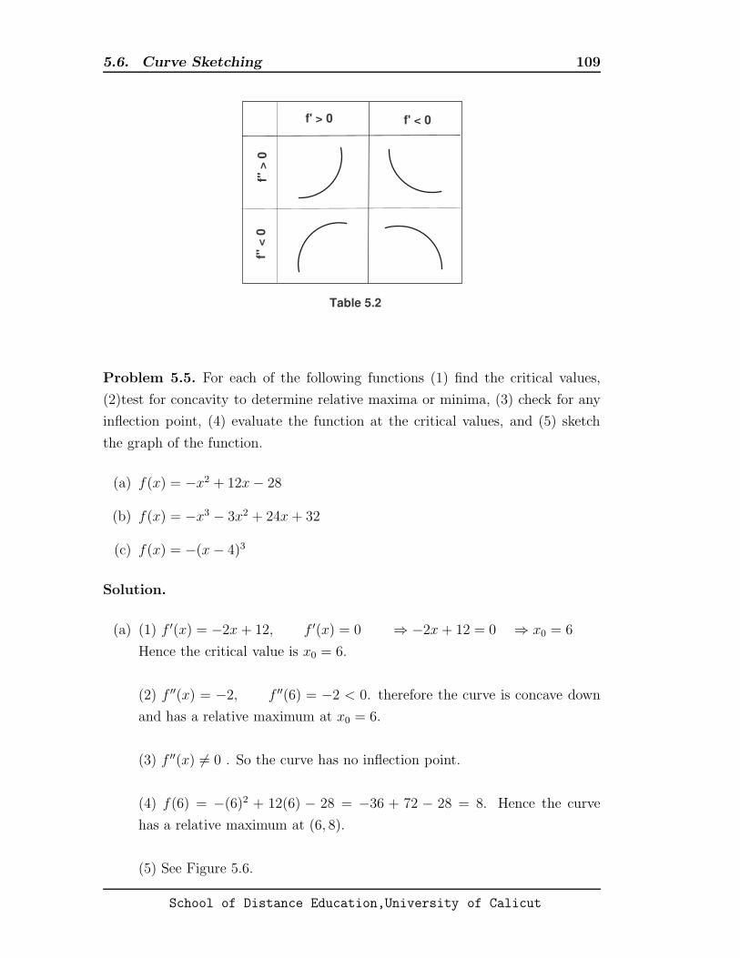
5.6. Curve Sketching 109
f' > 0
f" >
0
f' < 0
f" <
0
Table 5.2
Problem 5.5. For each of the following functions (1) find the critical values,
(2)test for concavity to determine relative maxima or minima, (3) check for any
inflection point, (4) evaluate the function at the critical values, and (5) sketch
the graph of the function.
(a) f(x) = −x2 + 12x− 28
(b) f(x) = −x3 − 3x2 + 24x+ 32
(c) f(x) = −(x− 4)3
Solution.
(a) (1) f ′(x) = −2x+ 12, f ′(x) = 0 ⇒ −2x+ 12 = 0 ⇒ x0 = 6
Hence the critical value is x0 = 6.
(2) f ′′(x) = −2, f ′′(6) = −2 < 0. therefore the curve is concave down
and has a relative maximum at x0 = 6.
(3) f ′′(x) 6= 0 . So the curve has no inflection point.
(4) f(6) = −(6)2 + 12(6) − 28 = −36 + 72 − 28 = 8. Hence the curve
has a relative maximum at (6, 8).
(5) See Figure 5.6.
School of Distance Education,University of Calicut

5.6. Curve Sketching 110
0 x
y
2
8
6
4
10
2 4 6 8 10
(6,8)
Figure 5.6
(b) (1) f ′(x) = −3x2 − 6x+ 24, f ′(x) = 0 implies,
−3x2 − 6x+ 24 = 0
−3(x2 + 2x− 8) = 0
−3(x− 2)(x+ 4) = 0
This is possible if (x− 2) or (x + 4) = 0, that is if x = 2 or x = −4 Hence
the critical values are x0 = 2 and x0 = −4.
(2) f ′′(x) = −6x− 6
f ′′(2) = −6(2)− 6 = −18 < 0
Therefore the curve is concave down and has a relative maximum at x0 = 2.
f ′′(−4) = −6(−4)− 6 = 18 > 0
Therefore the curve is concave up and has a relative minimum at x0 = −4.
(3) f ′′(x) = 0 ⇒ −6x− 6 = 0 ⇒ x = −1 .
Note that f(−1) = 6, So (−1, 6) is an inflection point.
(4) f(2) = 60 and f(−4) = −48. Hence the curve has a relative maxi-
mum at (2, 60) and relative minimum at (−4,−48).
(5) See Figure 5.7.
School of Distance Education,University of Calicut

5.6. Curve Sketching 111
0 x
y
20
60
40
1 2 3 4
(2,60)
-1-2-3-4-20
-40
-60
(-1,6)
(-4,-48)
Figure 5.7
(c) (1) f ′(x) = −3(x− 4)2, f ′(x) = 0 ⇒ −3(x− 4)2 = 0 ⇒ x0 = 4
Hence the critical value is x0 = 4.
(2)
f ′′(x) = −6(x− 4)
f ′′(4) = −6(4− 4) = 0
So the test is inconclusive. Continuing on to successively higher-order
derivatives in search of the first non zero derivatives,
f ′′′ = −6
f ′′′(4) = −6
Note that f(4) = 0. So (4, 0) is an inflection point.
(3) and (4) Now we test concavity to the left (x = 3) and right (x = 5) of
x = 4 to see which way the graph of the function curves:
Note that,
f ′′(3) = −6(3− 4) = 6 > 0
Hence the curve is concave upward at x = 3.
f ′′(5) = −6(5− 4) = −6 < 0
So the curve is concave downward at x = 5.
(5) Try yourself to draw the curve.
�
School of Distance Education,University of Calicut

5.6. Curve Sketching 112
Problem 5.6. Find the level of output at which profit π is maximized, given that
the total revenue R = 6400Q−20Q2 and total cost C = Q3−5Q2+400Q+52, 000
assume Q > 0.
Solution.
(1) Set up the profit function: π = R − C
π = 6400Q− 20Q2 − (Q3 − 5Q2 + 400Q+ 52, 000)
= 6400Q− 20Q2 −Q3 + 5Q2 − 400Q− 52, 000
= −Q3 − 15Q2 + 6000Q− 52, 000
(2) Take the first derivative, set it equal to zero, and solve for Q0 to find the
critical values. π′ = −3Q2 − 30Q+ 6000, π′ = 0 implies,
−3Q2 − 30Q+ 6000 = 0
−3(Q2 + 10Q− 2000) = 0
−3(Q+ 50)(Q− 40) = 0
This is possible if (Q+ 50) = 0 or (Q− 40) = 0, That is if Q = −50 or Q = 40
Hence the critical values are Q0 = −50 and Q0 = 40.
(3) Test the second order conditions
π′′ = −6Q− 30
we ignore the negative critical value. Note that,
π′′(40) = −6(40)− 30 = −270 < 0
Curve is concave down, and has a relative maximum at Q0 = 40. So the profit is
maximized at Q = 40 where,
π(40) = −(40)3 − 15(40)2 + 6000(40)− 52, 000 = 100, 000
�
School of Distance Education,University of Calicut
5.7. Exercises 113
5.7 Exercises
1. Determine whether the following functions are increasing, decreasing, or
stationary at x = 3:
(a) y = (4x− 5)2 (b)y =7x− 9
2x(x 6= 0)
2. Test to see if the following functions are concave upward or concave down-
ward at x = 5:
(a) y = 27+13x−3x2 (b) y = −x(x−10)2 (c) y =−4
x− 9(x 6= 9)
3. For each of the following functions (1) find the critical value(s) and (2)
determine whether at the critical value(s) the function is at a relative max-
imum or minimum :
(a) f(x) = −5x2 + 78x− 49 (b) f(x) = x4 − 72x2 + 7
4. For each of the following functions (1) find the critical values (2)test for
concavity to determine relative maxima or minima (3) check for any inflec-
tion point (4) evaluate the function at the critical values and (5) sketch the
graph of the function.
(a) f(x) = 4x2 − 24x+ 40 (b) f(x) = −(x− 3)4
(c) f(x) = 2x3 − 54x2 + 480x− 1300
5. Find the critical value(s) at which each of the follwoing function is opti-
mized and test the second-order condition to distinguish between relative
maximum and minimum:
(a) f(x) = 6x2 − 36x+ 25 (b) f(x) = −3x2 − 12x+ 57
(c) f(x) = 2x3 + 12x2 − 192x− 45 (d) −4x2 + 72x− 15
6. The concentration in milligrams per cubic centimeter of drug A in a person’s
bloodstream after t hours is given by
C(t) =0.18t
t2 + 3t + 25
Find when the concentration is strongest.
School of Distance Education,University of Calicut

Chapter 6Exponential and Logarithmic Functions
6.1 Exponential Functions
Earlier we dealt with power functions such as y = xa, which are composed of a
variable base x and a constant exponent a. In this chapter we encounter a new
function that is composed of a constant base a and a variable exponent x. It is
called an exponential function and is defined as
y = ax a > 0 and a 6= 1
For example f(x) = 2x is an exponential function and f(x) =
(
3
4
)x
is also an
exponential function.
There is a big difference between an exponential function and a polynomial.
The function p(x) = x3 is a polynomial. Here the variable, x, is being raised to
some constant power. The function f(x) = 3x is an exponential function; the
variable is the exponent. Exponential functions are used to express growth and
decay.
The following are some general characteristics of exponential functions.
Given y = ax, a > 0, a 6= 1 :
(a) The domain of the function is the set of all real numbers; the range of the
function is the set of all positive real numbers.
(b) For a > 1, the function is increasing and concave upward; for 0 < a < 1,
the function is decreasing and concave upward.
(c) at x = 0, y = 1, independently of the base.
114
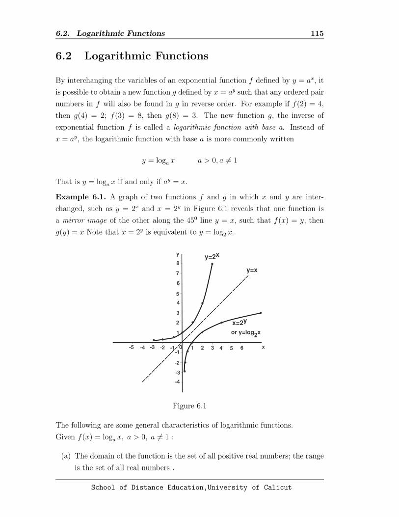
6.2. Logarithmic Functions 115
6.2 Logarithmic Functions
By interchanging the variables of an exponential function f defined by y = ax, it
is possible to obtain a new function g defined by x = ay such that any ordered pair
numbers in f will also be found in g in reverse order. For example if f(2) = 4,
then g(4) = 2; f(3) = 8, then g(8) = 3. The new function g, the inverse of
exponential function f is called a logarithmic function with base a. Instead of
x = ay, the logarithmic function with base a is more commonly written
y = loga x a > 0, a 6= 1
That is y = loga x if and only if ay = x.
Example 6.1. A graph of two functions f and g in which x and y are inter-
changed, such as y = 2x and x = 2y in Figure 6.1 reveals that one function is
a mirror image of the other along the 450 line y = x, such that f(x) = y, then
g(y) = x Note that x = 2y is equivalent to y = log2 x.
0 x
y
1 2 3 4-1-2-3-4
1
2
3
4
5 6-5
6
5
8
7
-1
-2
-3
-4
y=x
y=2x
x=2y
or y=log2x
Figure 6.1
The following are some general characteristics of logarithmic functions.
Given f(x) = loga x, a > 0, a 6= 1 :
(a) The domain of the function is the set of all positive real numbers; the range
is the set of all real numbers .
School of Distance Education,University of Calicut
6.3. Properties of Exponents and Logarithms 116
(b) For base a > 1, f(x) is increasing and concave down. For 0 < a < 1, f(x)
is decreasing and concave down.
(c) At x = 1, y = 0, independently of the base.
Example 6.2. .
(a) log2 16 = 4 is equivalent to 16 = 24.
(b) log25 5 = 12is equivalent to 5 = 251/24.
(c) log218= −3 is equivalent to 1
8= 2−3.
(d) 36 = 62 is equivalent to log6 36 = 2.
(e) 9 =√81 is equivalent to log81 9 = 1
2.
(f) 19= 3−2 is equivalent to log3
19= −2.
6.3 Properties of Exponents and Logarithms
Assuming a, b > 0; a, b 6= 1, and x and y any real number,
(a) ax · ay = ax+y
(b) a−x =1
ax
(c)ax
ay= ax−y
(d) (ax)y = axy
(e) ax · bx = (ab)x
(f) a−x =1
ax
(g)ax
bx=(a
b
)x
Letting x and y be any positive real numbers, n any real number, a any positive
real number, and a 6= 1,
(a) loga(xy) = loga x+ loga y
School of Distance Education,University of Calicut

6.3. Properties of Exponents and Logarithms 117
(b) logax
y= loga x− loga y
(c) loga xn = n loga x
(d) loga(n√x) =
1
n(loga x)
Problem 6.1. Change the following logarithms to their equivalent exponential
forms :
(a) log6 36 = 2
(b) log3 27 = 3
(c) log21
32= −5
(d) log81 3 =1
4
Solution.
(a) 36 = 62
(b) 27 = 33
(c)1
32= 2−5
(d) 3 = 811/4
�Problem 6.2. Change the following exponential forms to logarithmic forms :
(a) 49 = 72
(b)1
8= 2−3
(c) 4 = 641/3
(d) 27 = 93/2
Solution.
(a) log7 49 = 2
(b) log218= −3
School of Distance Education,University of Calicut
6.4. Natural Exponential and Logarithmic Functions 118
(c) log64 4 = 13
(d) log9 27 = 32
�
6.4 Natural Exponential and Logarithmic Func-
tions
The most commonly used base for exponential and logarithmic functions is the
irrational number e. e is defined as
limn→∞
(
1 +1
n
)n
= e
This limit when rounded to five decimal places equals 2.71828.
Exponential functions to base e are called natural exponential functions and
are written y = ex; logarithmic functions to base e are called natural logarithmic
functions and are expressed as y = loge x = ln x. Natural exponential and
logarithmic functions have the same general properties as other exponential and
logarithmic functions.
Problem 6.3. Convert the following natural logarithms into natural exponential
functions :
(a) ln 24 = 3.17805
(b) ln 0.75 = −0.28768
(c) ln 10 = 2.30258
Solution.
(a) 24 = e3.17805
(b) 0.75 = e−0.28768
(c) 10 = e2.30258
�
School of Distance Education,University of Calicut

6.4. Natural Exponential and Logarithmic Functions 119
Problem 6.4. Convert the following natural exponential expressions in to equiv-
alent natural logarithmic forms :
(a) 1.5 = e0.40547
(b) 25 = e3.21888
Solution.
(a) ln 1.5 = 0.40547
(b) ln 25 = 3.21888
�
Problem 6.5. Solve the following for x, y, or a by finding the equivalent expres-
sion :
(a) y = log20 400
(b) log5 x = 3
(c) loga 4 = 23
Solution.
(a) 400 = 20y ⇒ y = 2
(b) x = 53 = 125
(c) 4 = a2/3 ⇒ a = 43/2 = (43)1/2 = (64)1/2 = 8
�
Problem 6.6. Use the properties of logarithms to write the following expressions
as sums, differences, or products :
(a) loga 15x
(b) loga 28x3
(c) loga x3y4
School of Distance Education,University of Calicut
6.4. Natural Exponential and Logarithmic Functions 120
(d) loga8x
9y
(e) logax5
y3
Solution.
(a) loga 15x = loga 15 + loga x
(b) loga 28x3 = loga 28 + 3 loga x
(c) loga x3y4 = 3 loga x+ 4 loga y
(d) logax5
y3= loga x
5 − loga y3 = 5 loga x− 3 loga y
�
Problem 6.7. Use the properties of logarithms to write the following natural
logarithmic forms as sums, differences, or products :
(a) ln 45x2
(b) lnx3y4
(c) ln( 5√x)
(d) ln8x
9y
(e) ln
√
x5
y3
Solution.
(a) ln 45x2 = ln 45 + 2 lnx
(b) lnx3y4 = 3 lnx+ 4 ln y
(c) ln( 5√x) = ln(x)1/5 =
1
5ln x
(d) ln8x
9y= ln 8x− ln 9y = ln 8 + lnx− (ln 9 + ln y) = ln 8 + ln x− ln 9− ln y
School of Distance Education,University of Calicut

6.4. Natural Exponential and Logarithmic Functions 121
(e) ln
√
x5
y3= ln
(
x5
y3
)1/2
=1
2ln
x5
y3=
1
2(lnx5 − ln y3) =
1
2(5 ln x− 3 ln y)
�
Problem 6.8. Use the properties of exponents to simplify the following expo-
nential expressions, assuming a, b > 0 and a 6= b:
(a) ax · ay
(b) a2x · a3y
(c)a6x
a4y
(d)ax
by
(e)√a5x
(f) (ax)5y
Solution.
(a) ax · ay = ax+y (b) a2x · a3y = a2x+3y (c)a6x
a4y= a6x−4y
(d)ax
by=(a
b
)x
(e)√a5x = (a5x)1/2 = a(5/2)x (f) (ax)5y = a5xy
. �
Problem 6.9. Simplify the following natural exponential expressions:
(a) e7x · ey (b) (e4x)3 (c)e7x
e4x(d)
e3x
e7x
Solution.
(a) e7x · ey = e7x+y (b) (e4x)3 = e12x (c)e7x
e4x= e7x−4x = e3x
(d)e3x
e7x= e3x−7x = e−4x =
1
e4x. �
Problem 6.10. Simplify the following natural logarithmic expressions:
(a) ln 9 + ln x (b) ln x6 − ln x2 (c) ln 5− ln x+ ln 3 (d) 3 ln 14
(e) 12ln 49 (f) 2 ln 6− 1
2ln 16
School of Distance Education,University of Calicut

6.5. Solving Natural Exponential and Logarithmic Functions 122
Solution.
(a) ln 9 + ln x = ln 9x
(b) ln x6 − ln x2 = lnx6
x2= ln x4
(c) ln 5− ln x+ ln 3 = ln 5 + ln 3− ln x = ln 5 · 3− ln x = ln5.3
x= ln
15
x
(d) 3 ln 14=(
ln 14
)3
(e) 12ln 49 = ln 491/2 = ln 7
(f) 2 ln 6− 12ln 16 = ln 62 − ln 161/2 = ln 36− ln 4 = ln
36
4= ln 9
. �
6.5 Solving Natural Exponential and Logarith-
mic Functions
Natural exponential functions and natural logarithmic functions are inverses of
each other. Note that
eln a = a elnx = x eln f(x) = f(x)
Conversely,
ln ea = a ln ex = x ln ef(x) = f(x)
Problem 6.11. Simplify each of the following exponential expressions:
(a) e5 lnx (b) e3 lnx+2 ln y (c) e(1/2) lnx (d) e5 lnx−3 ln y
Solution.
(a) e5 lnx = elnx5
= x5
(b) e3 lnx+2 ln y = elnx3+ln y2 = elnx3 · eln y2 = x3y2
School of Distance Education,University of Calicut
6.5. Solving Natural Exponential and Logarithmic Functions 123
(c) e(1/2) lnx = elnx1/2= x1/2 =
√x
(d) e5 lnx−3 ln y = e5 lnx · e−3 ln y = elnx5 · e− ln y3 =elnx5
eln y3=
x5
y3. �
Problem 6.12. Simplify each of the following logarithmic expressions:
(a) ln ex (b) ln ex2
(c) 5 ln e3x2+4y
Solution.
(a) ln ex = x (b) ln ex2
= x2 (c) 5 ln e3x2+4y = 5(3x2 + 4y) = 15x2 + 20y
. �
Problem 6.13. Solve the following equations for x:
(a) 4 lnx− 10 = 0 (b) 3ex−4 = 24 (c) 2e3x = 3616 (d) 13ex
2
= 2701
Solution.
(a) (1) First solve algebraically for ln x,
4 ln x− 10 = 0
4 lnx = 10
ln x =10
4ln x = 2.5
(2) Then set both sides of the equation as exponents of e,
elnx = e2.5
⇒ x = e2.5
(b) (1) First solve algebraically for ef(x),
3ex−4 = 24
ex−4 =24
3ex−4 = 8
School of Distance Education,University of Calicut
6.5. Solving Natural Exponential and Logarithmic Functions 124
(2) Then take natural logarithm of both sides,
ln ex−4 = ln 8
Solving we get,
x− 4 = ln 8
⇒ x = 4 + ln 8
ln 8 = 2.07944,
⇒ x = 4 + 2.07944 = 6.07944
(c) (1) First solve algebraically for e3x,
2e3x = 3616
e3x = 1808
(2) Then take natural logarithm of both sides,
ln e3x = ln 1808
Solving we get,
3x = ln 1808
Using calculator or tables,
3x = 7.5
⇒ x = 2.5
(d) (1) First solve algebraically for ex2
,
1
3ex
2
= 2701
ex2
= 8103
(2) Then take natural logarithm of both sides,
ln ex2
= ln 8103
School of Distance Education,University of Calicut

6.6. Derivatives of Natural Exponential and Logarithmic Functions125
Solving we get,
x2 = ln 8103
Using calculator or tables,
x2 = 9
⇒ x = ±3
�
6.6 Derivatives of Natural Exponential and Log-
arithmic Functions
The following are rules of differentiation
1. Given f(x) = eg(x) where g(x) is a differentiable function of x, the derivative
is
f ′(x) = eg(x) · g′(x) (6.1)
2. Given f(x) = ln[g(x)] where g(x) is positive and differentiable function of
x, the derivative is
f ′(x) =1
g(x)· g′(x) = g′(x)
g(x)(6.2)
Problem 6.14. Find the derivatives of the following natural exponential func-
tions:
(a) f(x) = ex (b) f(x) = e3x (c) f(x) = e5x−2
(d) f(x) = e4x3
(e) f(x) = 4e2−x3
Solution.
(a) Let g(x) = x, then g′(x) = 1. Substituting in (6.1)
f ′(x) = ex · 1 = ex
School of Distance Education,University of Calicut

6.6. Derivatives of Natural Exponential and Logarithmic Functions126
(b) Let g(x) = 3x, then g′(x) = 3. Substituting in (6.1)
f ′(x) = e3x · 3 = 3e3x
(c) Let g(x) = 5x− 2, then g′(x) = 5. Substituting in (6.1)
f ′(x) = e5x−2 · 5 = 5e5x−2
(d) Let g(x) = 4x3, then g′(x) = 12x2. Substituting in (6.1)
f ′(x) = e4x3 · 12x2 = 12x2e4x
3
(e) Let g(x) = 2− x3, then g′(x) = −3x2. Substituting in (6.1)
f ′(x) = 4e2−x3 · −3x2 = −12x2e2−x3
�
Problem 6.15. Combine rules to differentiate the following functions:
(a) f(x) = 5xe3x (b) y = 6x3e4x (c) y = (e3x + e−5x)4
(d) f(x) =e−6x
1− 6x
Solution.
(a) f(x) = 5xe3x. By product rule,
f ′(x) = 5x(3e3x) + e3x(5) = 15xe3x + 5e3x = 5e3x(3x+ 1)
(b) y = 6x3e4x. By product rule,
y′ = 6x3(4e4x) + e4x(18x2) = 24x3e4x + 18x2e4x = 6x2e4x(4x+ 3)
(c) y = (e3x + e−5x)4. By the generalized power function rule or the chain rule,
y′ = 4(e3x + e−5x)3 · (3e3x − 5e−5x) = (12e3x − 20e−5x)(e3x + e−5x)3
School of Distance Education,University of Calicut
6.6. Derivatives of Natural Exponential and Logarithmic Functions127
(d) f(x) =e−6x
1− 6x. By the quotient rule,
f ′(x) =(1− 6x)(−6e−6x)− (e−6x)(−6)
(1− 6x)2
=(−6e−6x + 36xe−6x) + 6e−6x
(1− 6x)2
=−6e−6x + 36xe−6x + 6e−6x
(1− 6x)2
=36xe−6x
(1− 6x)2
�
Problem 6.16. Find the derivatives of the following natural logarithmic func-
tions:
(a) f(x) = ln x (b) f(x) = ln(−24x), x < 0 (c) f(x) = ln 5x4
(d) y = ln(7x2 − 15) (e) y = ln(x2 + 9x+ 12)
Solution.
(a) Let g(x) = x, then g′(x) = 1. Substituting in (6.2)
f ′(x) =g′(x)
g(x)=
1
x
(b) Let g(x) = −24x, then g′(x) = −24. From (6.2)
f ′(x) =g′(x)
g(x)=
−24
−24x=
1
x
(c) Let g(x) = 5x4, then g′(x) = 20x3. From (6.2)
f ′(x) =g′(x)
g(x)=
20x3
5x4=
4
x
School of Distance Education,University of Calicut

6.6. Derivatives of Natural Exponential and Logarithmic Functions128
(d) Let g(x) = 7x2 − 15, then g′(x) = 14x. Substituting in (6.2)
y′ =g′(x)
g(x)=
14x
7x2 − 15
(e) Let g(x) = x2 + 9x+ 12, then g′(x) = 2x+ 9. Substituting in (6.2)
y′ =g′(x)
g(x)=
2x+ 9
x2 + 9x+ 12
�
Problem 6.17. Show that if y = ln kx then y′ =1
xand if y = k ln x then y′ =
k
x
Solution. y = ln kx
Let g(x) = kx, then g′(x) = k. From (6.2)
y′ =g′(x)
g(x)=
k
kx=
1
x
y = k ln x, then
y′ = k · d
dx(lnx)
Let g(x) = x, then g′(x) = 1. From (6.2)
d
dx(ln x) =
g′(x)
g(x)=
1
x
⇒ y′ = k · 1x=
k
x
�
Problem 6.18. Combine rules to differentiate the following functions:
(a) y = ln2 x = (ln x)2 (b) y = ln2 4x3 = (ln 4x3)2 (c) y = e2x ln 3x
(d) y = ln(9x+ 4)2 6= [ln(9x+ 4)]2 (e) y = x5 ln x3 (f) y =x
lnx
School of Distance Education,University of Calicut

6.6. Derivatives of Natural Exponential and Logarithmic Functions129
Solution.
(a) By the chain rule,
y′ = 2(lnx)
(
1
x
)
=2 lnx
x
(b) By the chain rule,
y′ = 2(ln 4x3)
(
1
4x3
)
(12x2) =6 ln 4x3
x
(c) By the product rule,
y′ = e2x(
1
3x· 3)
+ (ln 3x)(e2x · 2)
= e2x(
1
x
)
+ 2e2x(ln 3x)
= e2x(
1
x+ 2 ln 3x
)
(d) Let g(x) = (9x+ 4)2, then g′(x) = 2(9x+ 4)(9) = 18(9x+ 4). Substituting
in (6.2),
y′ =18(9x+ 4)
(9x+ 4)2=
18
9x+ 4
(e) By the product rule,
y′ = x5
(
1
x3
)
(3x2) + (ln x3)(5x4) = 3x4 + (ln x3)(5x4)
(f) By the quotient rule,
y′ =(lnx)(1)− x(1/x)
(ln x)2=
ln x− 1
ln2 x
�
School of Distance Education,University of Calicut
6.7. Logarithmic Differentiation 130
6.7 Logarithmic Differentiation
The natural logarithm function and its derivative can be used to facilitate the
differentiation of product involving multiple terms. This process is called loga-
rithmic differentiation. In this method we take natural logarithm of both sides
before differentiation.
Problem 6.19. Find the derivative of
g(x) = (x3 − 2)(x2 − 3)(8x− 5) (6.3)
using logarithmic differentiation.
Solution.
(1) Take the natural logarithm of both sides ,
ln g(x) = ln[(x3 − 2)(x2 − 3)(8x− 5)]
= ln(x3 − 2) + ln(x2 − 3) + ln(8x− 5)
(2) Take the derivative of ln g(x),
d
dx[ln g(x)] =
g′(x)
g(x)=
3x2
x3 − 2+
2x
x2 − 3+
8
8x− 5(6.4)
(3) Solve algebraically for g′(x) in (6.4),
g′(x) =
(
3x2
x3 − 2+
2x
x2 − 3+
8
8x− 5
)
· g(x) (6.5)
(4) Then substitute (6.3) for g(x) in (6.5),
g′(x) =
(
3x2
x3 − 2+
2x
x2 − 3+
8
8x− 5
)
[(x3 − 2)(x2 − 3)(8x− 5)]
�
Problem 6.20. Use logarithmic differentiation to find the derivative of
g(x) =(3x5 − 4)(2x3 + 9)
7x4 − 5(6.6)
School of Distance Education,University of Calicut

6.8. Practical Applications of Exponential Functions 131
Solution.
(1) Take the natural logarithm of both sides,
ln g(x) = ln
[
(3x5 − 4)(2x3 + 9)
7x4 − 5
]
= ln(3x5 − 4) + ln(2x3 + 9)− ln(7x4 − 5)
(2) Take the derivative of ln g(x),
d
dx[ln g(x)] =
g′(x)
g(x)=
15x4
3x5 − 4+
6x2
2x3 + 9− 28x3
7x4 − 5(6.7)
(3) Solve algebraically for g′(x) in (6.7),
g′(x) =
(
15x4
3x5 − 4+
6x2
2x3 + 9− 28x3
7x4 − 5
)
· g(x) (6.8)
(4) Then substitute (6.6) for g(x) in (6.8),
g′(x) =
(
15x4
3x5 − 4+
6x2
2x3 + 9− 28x3
7x4 − 5
)
· (3x5 − 4)(2x3 + 9)
7x4 − 5
�
6.8 Practical Applications of Exponential Func-
tions
Exponential functions are used in business, economics, and each of the different
sciences to express rates of growth and decay, such as discrete and continuous
interest compounding and discounting; the growth of human, insect, and animal
populations; patterns and speed of learning and forgetting and rate of decay of
elements and organisms.
We know that compound interest arises when interest is added to the principal
of a deposit or loan, so that, from that moment on, the interest that has been
added also earns interest. This addition of interest to the principal is called com-
pounding. Interest Compounding is generally expressed in terms of exponential
functions. A person lending out a principal P at interest rate r under terms of
School of Distance Education,University of Calicut

6.8. Practical Applications of Exponential Functions 132
annual compounding for example, will have a value A at the end of one year equal
to,
A1 = P + rP = P (1 + r)
At the end of two years, he will have A1 plus interest on A1,
A2 = A1 + rA1 = P (1 + r) + r[P (1 + r)] = P (1 + r)[1 + r] = P (1 + r)2
At the end of t years, following the same procedure,
At = P (1 + r)t (6.9)
If the interest is compounded m times a year with the person receiving (r/m)
interest m times during the course of a year, at the end of t years,
At = P(
1 +r
m
)mt
(6.10)
If the interest is compounded continuously so that m → ∞ then
At = Pert (6.11)
Problem 6.21. Find the value A of a principal P=$ 10,000 set out at an interest
rate r = 8% for time t = 3 years when compounded (a) annually, (b) quarterly
(c) monthly, and (d) continuously
Solution.
(a) Here P = 10, 000, r = 8% = 0.08, t = 3 ; substituting these values in
(6.9) and using the yx key of a calculator to estimate exponential functions
throughout,
A = 10, 000(1 + 0.08)3 = 10, 000(1.25971) = 12, 597.10
(b) Substituting in (6.10) where m = 4 for quarterly compounding,
A = 10, 000
(
1 +0.08
4
)4(3)
= 10, 000(1 + 0.02)12 = 12, 682.40
School of Distance Education,University of Calicut

6.8. Practical Applications of Exponential Functions 133
(c) Now substituting m = 12 in (6.10) for monthly compounding,
A = 10, 000
(
1 +0.08
12
)12(3)
= 10, 000(1 + 0.0067)36 = 12, 702.40
(d) Finally using (6.11) for continuous compounding,
A = 10, 000e(0.08)3 = 10, 000e0.24
= 10, 000(1.27125) = 12, 712.50
�
Problem 6.22. Find the value A of a principal P=$ 100 set out at an interest rate
r = 8% for time t = 1 year when compounded (a) annually, (b) semi-annually, (c)
quarterly, and (d) continuously; (e) distinguish between the nominal and effective
rates of interest. Use a calculator for exponential expressions.
Solution.
(a) Here P = 100, r = 8% = 0.08, t = 1; substituting these values in (6.9) and
using the yx key of a calculator to estimate exponential functions through-
out,
A = 100(1 + 0.08)1 = 100(1.08) = 108
(b) Substituting in (6.10) with m = 2 for semi-annually compounding,
A = 100
(
1 +0.08
2
)2(1)
= 100(1 + 0.04)2 = 108.16
(c) Now substituting m = 4 in (6.10) for quarterly compounding,
A = 100
(
1 +0.08
4
)4(1)
= 100(1 + 0.02)4 = 108.24
(d) Finally using (6.11) for continuous compounding,
A = 100e(0.08)(1) = 100e0.08 = 108.33
School of Distance Education,University of Calicut

6.8. Practical Applications of Exponential Functions 134
(e) In all four instances the stated or nominal interest rate is the same, namely
8%; the actual interest earned, however, varies according to the type of
compounding. The effective interest rate on multiple compoundings is the
comparable rate the bank would have to pay if interest were paid only once
a year; that is 8.16% to equal semi-annual compounding, 8.24 % to equal
quarterly compounding, and 8.33% to equal continuous compounding.
�
Problem 6.23. Find the value A of a principal P=$ 2,000 set out at an interest
rate r = 6% for time t = 5 years when compounded (a) annually, (b) semi-
annually, (c) quarterly, and (d) continuously.
Solution.
(a) Here P = 2, 000, r = 6% = 0.06, t = 5; substituting these values in (6.9) and
using the yx key of a calculator to estimate exponential functions through-
out,
A = 2, 000(1 + 0.06)5 = 2, 000(1.06)5 = 2, 676.45
(b) From (6.10) with m = 2,
A = 2, 000
(
1 +0.06
2
)2(5)
= 2, 000(1 + 0.03)10 = 2, 687.83
(c) From (6.10) with m = 4,
A = 2, 000
(
1 +0.06
4
)4(5)
= 2, 000(1 + 0.015)20 = 2, 693.71
(d) From (6.11),
A = 2, 000e(0.06)(5) = 2, 000e0.3 = 2, 699.72
�
Problem 6.24. How many years t will it take a sum of money P to double at
8% interest compounded annually?
School of Distance Education,University of Calicut
6.8. Practical Applications of Exponential Functions 135
Solution.
A = P (1 + 0.08)t
For money to double, A = 2P . Substitute for A,
2P = P (1 + 0.08)t
Divided by P ,
2 = (1 + 0.08)t
Take the natural log,
ln 2 = ln(1 + 0.08)t
ln 2 = t ln(1 + 0.08)
ln 2 = t ln 1.08
0.69315 = 0.07696t
Divide by 0.07696,
t = 9 years
�
Problem 6.25. How long it take money to treble at 10% interest compounded
quarterly?
Solution. From (6.10),
A = P
(
1 +0.10
4
)4(t)
= P (1 + 0.025)4t
For money to treble, A = 3P . Substitute for A,
3P = P (1 + 0.025)4t
3 = (1 + 0.025)4t
Take the natural log,
ln 3 = ln(1 + 0.025)4t
ln 3 = 4t ln(1 + 0.025)
School of Distance Education,University of Calicut

6.8. Practical Applications of Exponential Functions 136
ln 3 = 4t ln 1.025
1.09861 = 4(0.02469)t
1.09861 = 0.09876t
Divide by 0.09876,
t = 11.12 years
. �
Discounting is the process of determining the present value P of a sum of money
A to be received in the future.
Problem 6.26. Find the formula for discounting under (a) annual compounding,
(b) multiple compounding and (c) continuous compounding.
Solution.
(a) Under annual compounding,
A = P (1 + r)t
Solve for P ,
P =A
(1 + r)t= A(1 + r)−t (6.12)
(b) Under multiple compounding,
A = P(
1 +r
m
)mt
Solve for P ,
P =A
(
1 +r
m
)mt = A(
1 +r
m
)−mt
(6.13)
(c) For continuous compounding,
A = Pert
School of Distance Education,University of Calicut

6.8. Practical Applications of Exponential Functions 137
Solve for P ,
P = Ae−rt (6.14)
�Problem 6.27. Find the present value of $1000 to be paid five years from now
when the current interest rate is 10% if interest is compounded (a) annually, (b)
quarterly, and (c) continuously.
Solution.
(a) From (6.12),
P = A(1 + r)−t
Substituting,
P = 1000(1 + 0.10)−5
Using calculator,
P = 1000(0.62092) = 620.92
(b) From (6.13),
P = A(
1 +r
m
)−mt
Substituting,
P = 1000
(
1 +0.10
4
)−4(5)
= 1000(1 + 0.025)−20
Using calculator,
P = 1000(0.61027) = 610.27
(c) From (6.14),
P = Ae−rt
Substituting,
P = 1000e−(0.10)(5) = 1000e−0.5
= 1000(0.60653) = 606.53
�
School of Distance Education,University of Calicut

6.8. Practical Applications of Exponential Functions 138
Problem 6.28. Find the present value of $1200 to be paid in 10 years from now
when the current interest rate is 8% if interest is compounded (a) annually, (b)
quarterly, and (c) continuously.
Solution.
(a) From (6.12),
P = A(1 + r)−t
Substituting,
P = 1200(1 + 0.08)−10
Using calculator,
P = 1200(0.46319) = 555.83
(b) From (6.13),
P = A(
1 +r
m
)−mt
Substituting,
P = 1200
(
1 +0.08
4
)−4(10)
= 1200(1 + 0.02)−40
Using calculator,
P = 1200(0.45289) = 543.47
(c) From (6.14),
P = Ae−rt
Substituting,
P = 1200e−(0.08)(10) = 1000e−0.8
= 1200(0.44933) = 539.19
�
School of Distance Education,University of Calicut

6.8. Practical Applications of Exponential Functions 139
Problem 6.29. Find the percentage or relative rate of growth G for each of the
following functions using the derivative of the natural logarithm of the function:
(a) f(t) = 5t2 (b) f(t) =t
4t
Solution.
(a) First take the natural logarithm of both sides,
ln f(t) = ln 5t2
ln f(t) = ln 5 + 2 ln t
Then take derivative, note that ln 5 is a constant,
G =d
dtln f(t) =
f ′(t)
f(t)= 0 + 2
(
1
t
)
=2
t
(b) First take the natural logarithm of both sides,
ln f(t) = lnt
4t
ln f(t) = ln t− t ln 4
Then take derivative, note that ln 4 is a constant,
G =d
dtln f(t) =
f ′(t)
f(t)=
1
t− ln 4
�
Problem 6.30. Find the relative growth rate G of sales at t = 4, given S(t) =
100000e0.5√t.
Solution. First take the natural logarithm of both sides,
lnS(t) = ln 100000 + 0.5√t
lnS(t) = ln 100000 + 0.5t1/2
School of Distance Education,University of Calicut

6.8. Practical Applications of Exponential Functions 140
Then take derivative,
G =d
dtlnS(t) =
S ′(t)
S(t)= 0.5
(
1
2
)
t−1/2 =0.25√
t
At t = 4,
G =0.25√
4= 0.125 = 12.5%
�
Problem 6.31. Derive the formula for finding the effective rate of interest re for
multiple compondings when t > 1.
Solution. From the explanation of the effective rate of interest in Problem 6.22
(e), we can write
P (1 + re)t = P
(
1 +r
m
)mt
Dividing by P and taking tth root of each side,
1 + re =(
1 +r
m
)m
re =(
1 +r
m
)m
− 1 (6.15)
For continuous compounding,
P (1 + re)t = Pert
1 + re = er
re = er − 1 (6.16)
�
Problem 6.32. Find the effective rate of interest for P = $2000 ar r = 6% when
compounded (a) semiannually, (b) quarterly, (c) continuously, noting that P and
t do not matter.
Solution.
(a) From (6.15),
re =(
1 +r
m
)m
− 1
School of Distance Education,University of Calicut

6.9. Exercises 141
Substituting,
re =
(
1 +.06
2
)2
− 1
= (1 + 0.03)2 − 1
= 1.0609− 1 = 0.0609 = 6.09%
(b)
re =
(
1 +.06
4
)4
− 1
= (1 + 0.015)4 − 1
= 1.06136− 1 = 0.06136 = 6.136%
(c) From (6.16),
re = er − 1
Substituting,
re = e0.06 − 1 = 1.061837− 1 = 0.061837 = 6.1837%
�
6.9 Exercises
1. Solve the following for x, y, a by finding the equivalent expression:
(a) y = log2116
(b) loga 4 = 23
(c) log81 x = 34
2. Use the properties of logarithms to write the following as sums, differences,
or products:
(a) loga u2v−3
(b) loga3√x
School of Distance Education,University of Calicut

6.9. Exercises 142
3. Use the properties of logarithms to write the following natural logarithmic
forms as sums, differences, or products:
(a) lnx3
y4
(b) ln4x
7y
(c) ln(x3√y)
4. Differentiate the following functions:
(a) y = (e−2x)3
(b) y =e7x − 1
e7x + 1
(c) y = ln(9x2 + 5)
(d) y = 15 lnx
(e) y = e2x ln 3x
(f) y = ln2(21x+ 8)
5. Use logarithmic differentiation to find the derivative of
g(x) = (x4 + 7)(x5 + 6)(x3 + 2)
6. Find the effective rate of interest for P = $500 ar r = 12% when com-
pounded (a) semiannually, (b) quarterly, (c) continuously, noting that P
and t do not matter.
7. Find the relative growth of profits at t = 8, given π(t) = 2, 50, 000e1.2t1/3
School of Distance Education,University of Calicut
Chapter 7Integration
7.1 Antidifferentiation
Integration is the inverse operation of differentiation.Reversing the process of
differentiation and finding the original function from the derivative is called inte-
gration or antidifferentiation. Suppose the derivative of F (x) is F ′(x).Then F (x)
is called the integral or antiderivative of F ′(x).
Let f(x) = F ′(x), the antiderivative of f(x) is expressed as
∫
f(x)dx = F (x) + c
Here the left-hand side of the equation is read as “the indefinite integral of f of
x with respect to x ”. The symbol∫
is an integral sign, f(x) is the integrand,
and c is the constant of integration. The integral is called an indefinite integral
because its value is not fully determined until the end points are specified. This
ambiguity is dealt with by the addition of the constant c at the end.
7.2 Rules for Indefinite IntegralsThe following rules for indefinite integrals are obtained by reversing the corre-
sponding rules of differentiation.
RULE 1. The integral of a constant k is
∫
kdx = kx+ c (7.1)
143
7.2. Rules for Indefinite Integrals 144
RULE 2. The integral of 1, written simply as dx is
∫
dx = x+ c (7.2)
RULE 3. The integral of a power function xn, where n 6= −1, is
∫
xndx =xn+1
n+ 1+ c n 6= −1 (7.3)
RULE 4. The integral of x−1, or (1/x), is
∫
x−1dx = ln |x|+ c x 6= 0 (7.4)
Note that if x > 0,∫
x−1dx = ln x+ c
RULE 5. The integral of a natural exponential function is
∫
ekxdx =ekx
k+ c (7.5)
RULE 6. The integral of a constant times a function equals the constant times
the antiderivative of the function.
∫
kf(x)dx = k
∫
f(x)dx+ c (7.6)
RULE 7. The integral of the sum or difference of two or more functions equals
the sum or difference of their integrals.
∫
[f(x)± g(x)]dx =
∫
f(x)dx±∫
g(x)dx (7.7)
RULE 8. The integral of the negative of a function equals the negative of the
integral of the function
∫
−f(x)dx = −∫
f(x)dx (7.8)
School of Distance Education,University of Calicut

7.2. Rules for Indefinite Integrals 145
Example 7.1. The rules for indefinite integrals are illustrated below.
(a)∫
5dx = 5x+ c [Rule 1]
(b)∫
x4dx =x4+1
4 + 1+ c =
x5
5+ c [Rule 3]
(c)∫
5x4dx = 5∫
x4dx [Rule 6]
. = 5
(
x4+1
4 + 1+ c1
)
[Rule 3]
. = 5
(
x5
5+ c1
)
= x5 + 5c1
. = x5 + c
where c1 and c are arbitrary constants and 5c1 = c.
(d)∫
x−3dx =x−3+1
−3 + 1+ c = −x−2
2+ c [Rule 3]
(e)∫
e5xdx =e5x
5+ c [Rule 5]
(f)∫
(1− x)dx =∫
dx−∫
xdx [Rule 8]
. = x− x2
2+ c [Rule 3]
Problem 7.1. Find the following indefinite integrals:
(a)
∫
7dx
(b)
∫
−12dx
(c)
∫
x5dx
(d)
∫
4
x5dx
(e)
∫
(20x4 − 8x3)dx
(f)
∫ √xdx
School of Distance Education,University of Calicut

7.2. Rules for Indefinite Integrals 146
(g)
∫
12e−3tdt
(h)
∫
2
xdx
(i)
∫
1
x+ 9dx
(j)
∫ √x+ 5dx
Solution.
(a)
∫
7dx = 7x+ c
(b)
∫
−12dx = −∫
12dx = −12x+ c
(c)
∫
x5dx =x6
6+ c
(d)
∫
4
x5dx = 4
∫
1
x5dx
= 4
∫
x−5dx
= 4
(
x−5+1
−5 + 1+ c1
)
= 4
(
x−4
−4+ c1
)
= −x−4 + 4c1
= − 1
x4+ c where c = 4c1
(e)
∫
(20x4 − 8x3)dx =
∫
20x4dx−∫
8x3dx
= 20
∫
x4dx− 8
∫
x3dx
= 20 · x5
5− 8 · x
4
4+ c
=4x5
5− 2x4 + c
School of Distance Education,University of Calicut
7.2. Rules for Indefinite Integrals 147
(f)
∫ √xdx =
∫
x1/2dx
=x1/2+1
1/2 + 1+ c
=x3/2
3/2+ c
=2
3x3/2 + c
(g)
∫
12e−3tdt = 12
∫
e−3tdt = 12
(
e−3t
−3+ c1
)
= −4e−3t + 12c1 = −4e−3t + c
(h)
∫
2
xdx = 2
∫
1
xdx = 2 ln |x|+ c = ln x2 + c
(i)
∫
1
x+ 9dx =
∫
(x+ 9)−1dx = ln |x+ 9|+ c
(j)
∫ √x+ 5dx =
∫
(x+ 5)1/2dx
=(x+ 5)1/2+1
1/2 + 1+ c
=(x+ 5)3/2
3/2+ c
=2
3(x+ 5)3/2 + c
�Problem 7.2. Find the antiderivative for each of the following :
(a)
∫
(25x1/4 + 16x1/3)dx, given F (0) = 19
(b)
∫
(16e2t + 15e−3t)dt, given F (0) = 9
(c)
∫
(4x−1 + 5x−2)dx, given F (1) = 3
School of Distance Education,University of Calicut

7.2. Rules for Indefinite Integrals 148
Solution.
(a)∫
(25x1/4 + 16x1/3)dx =
∫
25x1/4dx+
∫
16x1/3dx
= 25
∫
x1/4dx+ 16
∫
x1/3dx
= 25
(
x1/4+1
1/4 + 1
)
+ 16
(
x1/3+1
1/3 + 1
)
+ c
= 25
(
x5/4
54
)
+ 16
(
x4/3
43
)
+ c
= 25
(
4
5
)
x5/4 + 16
(
3
4
)
x4/3 + c
= 20x5/4 + 12x4/3 + c
⇒ F (x) = 20x5/4 + 12x4/3 + c
Given F (0) = 19, ⇒ 19 = 20(0)5/4 + 12(0)4/3 + c = 0 + c = c ⇒ c = 19
∴ F (x) = 20x5/4 + 12x4/3 + 19
(b)∫
(16e2t + 15e−3t)dt =
∫
16e2tdt+
∫
15e−3tdt
= 16
∫
e2tdt+ 15
∫
e−3tdt
= 16
(
e2t
2
)
+ 15
(
e−3t
−3
)
+ c
= 8e2t − 5e−3t + c
⇒ F (t) = 8e2t − 5e−3t + c
School of Distance Education,University of Calicut
7.3. The Definite Integral 149
Given F (0) = 9, ⇒ 9 = 8e2(0) − 5e−3(0) + c ⇒ 9 = 8− 5 + c = 3 + c
⇒ c = 9− 3 = 6
∴ F (t) = 8e2t − 5e−3t + 6
(c) Try your self . Answer is
F (x) = 4 ln x− 5
x+ 8
�
7.3 The Definite Integral
The area under the curve y = f(x) between x = a and x = b is the definite
integral of f(x) over the interval a to b. We write,
Area A =
∫ b
a
f(x)dx
We read right-hand side as “the integral from a to b of f of x dx ”; a is called
the lower limit of integration, b the upper limit of integration.
7.4 The Fundamental Theorem of Calculus
If f(x) = F ′(x) then
∫ b
a
f(x)dx = F (x)|ba = F (b)− F (a) (7.9)
where the symbol |ba or ]ba or [· · · ]ba indicates that b and a are to be substituted
successively for x.
Problem 7.3. Evaluate the following definite integrals:
(a)
∫ 5
1
4xdx
(b)
∫ 4
2
(9x2 + 6)dx
School of Distance Education,University of Calicut
7.4. The Fundamental Theorem of Calculus 150
Solution.
(a)
∫ 5
1
4xdx = 2x2∣
∣
5
1= 2(5)2 − 2(1) = 50− 2 = 48
(b)
∫ 4
2
(9x2 + 6)dx = [3x3 + 6x]42 = [3(4)3 + 6(4)]− [3(2)3 + 6(2)] = 180
�
Problem 7.4. Evaluate the following definite integrals:
(a)
∫ 9
1
12√xdx
(b)
∫ 1
0
et/2dt
(c)
∫ 2
0
(7 + x)3dx
Solution.
(a)
∫ 9
1
12√xdx =
∫ 9
1
12x1/2dx = 8x3/2∣
∣
9
1= 8(9)3/2− 8(1)3/2 = 8(27)− 8 = 208
(b)
∫ 1
0
et/2dt =
[
et/2
1/2
]1
0
=[
2et/2]1
0= 2e1/2 − 2e0/2 = 2e1/2 − 2 = 2(e1/2 − 1)
(c)
∫ 2
0
(7 + x)3dx =
[
(7 + x)4
4
]2
0
=(7 + 2)4
4− (7 + 0)4
4=
94 − 74
4= 1040
�
Problem 7.5. Determine the area under the curve y = 20− 4x over the
interval 0 to 5.
Solution.
Area A =
∫ 5
0
(20− 4x)dx = [20x− 2x2]50 = 20(5)− 2(5)2 = 100− 50 = 50
�
School of Distance Education,University of Calicut
7.5. Properties of Definite Integrals and Area Between Curves 151
7.5 Properties of Definite Integrals and Area
Between Curves
1. Reversing the order of the limits of integration changes the sign of the
definite integral.
∫ b
a
f(x)dx = −∫ a
b
f(x)dx (7.10)
2. If the upper limit of integration equals the lower limit of integration, the
value of the definite integral is zero.
∫ a
a
f(x)dx = F (a)− F (a) = 0 (7.11)
3. The definite integral can be expressed as the sum of component sub inte-
grals.
∫ c
a
f(x)dx =
∫ b
a
f(x)dx+
∫ c
b
f(x)dx a ≤ b ≤ c (7.12)
4.
∫ b
a
f(x)dx±∫ b
a
g(x)dx =
∫ b
a
[f(x)± g(x)]dx (7.13)
5.
∫ b
a
kf(x)dx = k
∫ b
a
f(x)dx (7.14)
Problem 7.6. Draw graphs for the following functions and evaluate the area
between the curves over the stated interval
(a) y = 7− x2 and y = 3 from x = −2 to x = 2.
(b) y = 10 and y = x2 + 1 from x = −3 to x = 3.
Solution.
(a) The desired area is the area under the curve specified by y = 7 − x2 from
x = −2 to x = 2, minus the area under the curve specified by y = 3 from
x = −2 to x = 2.
School of Distance Education,University of Calicut

7.5. Properties of Definite Integrals and Area Between Curves 152
2
0 x
y
1 2 3 4-1-2-3-4
1
5
xxxxxxxxxxxxxxxxxxxxxxxxxxxxxxxxxxxxxxxxxxxxxxxxxxxxxxxxxxxxxxxxxxxxxxxxxxxxxxxxxxxxxxxxxxxxxxxxxxxxxxxxxxxxxxxxxxxxxxxxxxxxxxxxxxxxxxxxxxxxxxxxxxxxxxxxxxxxxxxxxxxxxxxxxxxxxxxxxxxxxxxxxxxxxxxxxxxxxxxxxxxxxxxxxxxxxxxxxxxxxxxxxxxxxxxxxxxxxxxxxxxxxxxxxxxxxxxxxxxxxxxxxxxxxxxxxxxxxxxxxxxxxxxxxxxxxxxxxxxxxxxxxx
y = 7- x2
y=33
4
6
5
xx
8
7
Figure 7.1
A =
∫ 2
−2
(7− x2)dx−∫ 2
−2
3dx
=
∫ 2
−2
[(7− x2)− (3)]dx
=
∫ 2
−2
(7− x2 − 3)dx
=
∫ 2
−2
(4− x2)dx
=
[
4x− x3
3
]2
−2
=
(
4(2)− (2)3
3
)
−(
4(−2)− (−2)3
3
)
=
(
8− 8
3
)
−(
−8 − −8
3
)
=
(
8− 8
3
)
−(
−8 +8
3
)
=
(
16
3
)
−(−16
3
)
=
(
16
3+
16
3
)
=32
3
School of Distance Education,University of Calicut

7.5. Properties of Definite Integrals and Area Between Curves 153
So the area between the curves is A =32
3.
(b) .
0 x
y
1 2 3 4-1-2-3-4 5
y = x2+1
y=10
xxxxxxxxxxxxxxxxxxxxxxxxxxxxxxxxxxxxxxxxxxxxxxxxxxxxxxxxxxxxxxxxxxxxxxxxxxxxxxxxxxxxxxxxxxxxxxxxxxxxxxxxxxxxxxxxxxxxxxxxxxxxxxxxxxxxxxxxxxxxxxxxxxxxxxxxxxxxxxxxxxxxxxxxxxxxxxxxxxxxxxxxxxxxxxxxxxxxxxxxxxxxxxxxxxxxxxxxxxxxxxxxxxxxxxxxxxxxxxxxxxxxxxxxxxxxxxxxxxxxxxxxxxxxxxxxxxxxxxxxxxxxxxxxxxxxxxxxxxxxxxxxxxxxxxxxxxxxxxxxxxxxxxxxxxxxxxxxxxxxxxxxxxxxxxxxxxxxxxxxxxxxxxxxxxxxxxxxxxxxxxxxxxxxxxxxxxxxxxxxxxxxxxxxxxxxxxxxxxxxxxxxxxxxxxxxxxxxxxxxxxxxxxxxxxxxxxxxxxxxxxxxxxxxxxxxxxxxxxxxxxxxxxxxxxxxxxxxxxxxxxxxxxxxxxxxxxxxxxxx
2
4
6
10
xx
8
12
Figure 7.2
Required area
A =
∫ 3
−3
10dx−∫ 3
−3
(x2 + 1)dx
=
∫ 3
−3
[10− (x2 + 1)]dx =
∫ 3
−3
(9− x2)dx
=
[
9x− x3
3
]3
−3
=
[
9(3)− (3)3
3
]
−[
9(−3)− (−3)3
3
]
= 36
So the area between the curves is A = 36.
�
School of Distance Education,University of Calicut

7.6. Average Value of a Function and The Volume of a Solid of
Revolution 154
7.6 Average Value of a Function and The Vol-
ume of a Solid of Revolution
If f(x) is a continuous function on the interval [a, b], the average value m of f(x)
on this interval is defined as
m =1
b− a
∫ b
a
f(x)dx (7.15)
If a continuous function f(x) from x = a to x = b is rotated around the x-axis,
a solid of revolution is created. The volume of the solid of revolution V can be
expressed mathematically as
V =
∫ b
a
π[f(x)]2dx (7.16)
Problem 7.7. Find the average valuem of the following functions on the interval
[a, b]:
(a) f(x) = x2 − 1; a = 0, b = 3
(b) f(x) =1√x+ 3
; a = 1, b = 6
(c) f(x) = ex/6; a = 0, b = 6
Solution.
(a) From (7.15), m =1
b− a
∫ b
a
f(x)dx
Substituting we get,
m =1
3− 0
∫ 3
0
(x2 − 1)dx
=1
3
[
x3
3− x
]3
0
=1
3
[(
(3)3
3− 3
)
−(
(0)3
3− 0
)]
=1
3(9− 3) =
6
3= 2
School of Distance Education,University of Calicut
7.6. Average Value of a Function and The Volume of a Solid of
Revolution 155
Average value m = 2.
(b) From (7.15), m =1
b− a
∫ b
a
f(x)dx
Substituting we get,
m =1
6− 1
∫ 6
1
1√x+ 3
dx
=1
5
∫ 6
1
(x+ 3)−1/2dx
=1
5
[
(x+ 3)1/2
1/2
]6
1
=1
5[2(x+ 3)1/2]61 =
2
5[(x+ 3)1/2]61
=2
5[91/2 − 41/2] =
2
5(3− 2) =
2
5
Average value m =2
5.
(c) From (7.15), m =1
b− a
∫ b
a
f(x)dx
m =1
6− 0
∫ 6
0
ex/6dx
=1
6
[
ex/6
1/6
]6
0
=1
6
[
6ex/6]6
0
=[
ex/6]6
0= e(1) − e(0)
= e− 1 = 1.71828
Average value m = 1.71828.
�
School of Distance Education,University of Calicut

7.7. Practical Applications 156
Problem 7.8. Find the volume V of the solid of revolution generated by revolving
around the x-axis the regions under each of the following curves.
(a) f(x) = 5x2 ; a = 1, b = 3
(b) f(x) =√9− x2 ; a = −3, b = 3
Solution.
(a) From (7.16),
V =
∫ b
a
π[f(x)]2dx
Substituting,
V =
∫ 3
1
π[(5x2)]2dx
Squaring and rearranging constants,
V =
∫ 3
1
π(25x4)dx = 25π
∫ 3
1
x4dx = 25π
[
1
5x5
]3
1
= 5π(243− 1) = 1210π.
(b) From (7.16),
V =
∫ b
a
π[f(x)]2dx
Substituting,
V =
∫ 3
−3
π[√9− x2]2dx
Squaring and rearranging constants,
V =
∫ 3
−3
π(9− x2)dx = π
[
9x− x3
3
]3
−3
= π[(27− 9)− (−27 + 9)] = 36π.
�
7.7 Practical Applications
Problem 7.9. A person’s rate of reaction or sensitivity to a specific drug t hours
after it is administered is given by
S ′(t) =3
t+
4
t2
School of Distance Education,University of Calicut

7.7. Practical Applications 157
where S is measured is suitable units. Find the strength of the total reaction
from t = 1 to t = 8.
Solution.
S(t) =
∫ 8
1
(3t−1 +4t−2)dt =
(
3 ln t− 4
t
)∣
∣
∣
∣
8
1
=
(
3 ln 8− 1
2
)
−(
3 ln 1− 4
1
)
≈ 9.7
�
Problem 7.10. A firm’s marginal cost function is C ′(x) = x2 − 4x + 110 with
x representing the number of units per day. Fixed costs are 340 a day. What is
the total cost C(x) of producing x units per day?
Solution.
C(x) =
∫
(x2 − 4x+ 110)dx =x3
3− 2x2 + 110x+ c
Substituting C(0) = 340,
340 =(0)3
3− 2(0)2 + 110(0) + c ⇒ c = 340
and
C(x) =x3
3− 2x2 + 110x+ 340
�
Problem 7.11. A manufacturer’s marginal profit is π′ = −3x2+80x+140. Find
the profit π earned by increasing production from two units to four units.
Solution.
π(4)− π(2) =
∫ 4
2
(−3x2 + 80x+ 140)dx
. = (−x3 + 40x2 + 140x)∣
∣
4
2= 704
�
School of Distance Education,University of Calicut

7.8. Exercises 158
Problem 7.12. A zinc mine extracts ore at a rate of thousands of tons per year,
Z ′(t) = 18t − (22/√t). Find the total amount of ore extracted from year 0 to
year 9
Solution.
Z(t) =
∫ 9
0
(18t− 22t−1/2)dt = (9t2 − 44t1/2)∣
∣
9
0= 5, 97, 000 tons
�
Problem 7.13. According to engineer’s estimates, the cost of a new product is
C = 6√x+ 15. Find the average cost m of producing the first 64 units.
Solution. From (7.15),
m =1
b− a
∫ b
a
f(x)dx =1
64− 0
∫ 64
0
6√x+ 15dx
. =1
64
[
4x3/2 + 15x]64
0= 47
�
7.8 Exercises
1. Determine the following indefinite integrals:
(a)
∫
10et/2dt
(b)
∫
dx√xdx
(c)
∫
8
t5dt
(d)
∫
6(x− 15)−2dx
2. Evaluate the following definite integrals:
(a)
∫ 4
2
3x2dx
(b)
∫ 36
4
dx√xdx
School of Distance Education,University of Calicut

7.8. Exercises 159
(c)
∫ 1
0
12e−4tdt
(d)
∫ 5
1
3x−1
3. Draw graphs for the following functions and evaluate the area between the
curves over the stated interval.
(a) y = 7− x and y = 4x− x2 from x = 1 to x = 4
(b) y = 6− x and y = 4 from x = 0 to x = 5
(c) y = 10− 2x and y = x+ 1 from x = 0 to x = 4
(d) The area bounded by y = x2,y = 6x, and y = 8x − 2 from x = 0 to
x = 2
4. Find the average value m of the following functions on the interval [a, b]:
(a) f(x) = 2x+ 8; a = 3, b = 7
(b) f(x) =√x− 2; a = 6, b = 11
5. Find the volume V of the solid of revolution generated by revolving around
the x-axis the regions under each of the following curves:
(a) f(x) = 3x+ 2 ; a = 0, b = 4
(b) f(x) = e−1.5x ; a = 0, b = 1
6. A pipe on an offshore drilling platform is damaged ,spilling oil at a rate of
(35t+80) barrels per hour t. How many barrels will be leaked the first day?
7. A producer’s marginal cost is C ′(x) = 112x2 − x + 180. What is the total
cost C(x) of producing five extra units if three units are currently being
produced?
8. Find the producer’s surplus for the supply curve p = x2 + 4x + 60 at the
level x0 = 5, p0 = 85.
9. The population in millions of people for a newly emerging nation is P (t) =
18e0.032t. Find the average population m over the next 25 years.
School of Distance Education,University of Calicut

Chapter 8Multivariable Calculus
8.1 Functions of Several Variables
In this section, we extend the definition of a function of one variable to functions of
two or more variables. You will recall that a function was a rule which assigned
a unique value to each input value. It is going to be similar for two or more
variables. The only difference is that the input is not a value any more, it is
several values. z = f(x, y) is defined as a function of two independent variables if
there exists one and only one value of z in the range of f for each ordered pair of
real numbers (x, y) in the domain of f . Here z is the dependent variable, x and
y are the independent variables.
Example 8.1. If a firm produces one good x for which the cost function is
C(x) = 350+8x and another good y for which the cost function is C(y) = 225+6y,
the total cost to the firm can be expressed simply as
C(x, y) = 350 + 8x+ 225 + 6y = 575 + 8x+ 6y
Other examples of multi variable function include:
f(x, y) = x3 + 3xy + y2
z(x, y) = 5xy2
160

8.2. Partial Derivatives 161
Example 8.2. Multivariable functions can be evaluated for specific values of x
and y such as x = 2 and y = 4 by replacing x and y with the desired values.
Using the function from Example 8.1
C(2, 4) = 575 + 8(2) + 6(4) = 615
f(2, 4) = 23 + 3(2)(4) + 42 = 48
z(2, 4) = 5(2)(4)2 = 160
8.2 Partial Derivatives
Let z = f(x, y). The partial derivative of z with respect to x measures the
rate of change of z with respect to x while y is held constant. It is written
∂z/∂x, ∂f/∂x, fx(x, y), fx, or zx and is defined as
∂z
∂x= lim
∆x→0
f(x+∆x, y)− f(x, y)
∆x(8.1)
Similarly, the partial derivative of z with respect to y measures the rate of change
of z with respect to y while x is held constant. It is written ∂z/∂y, ∂f/∂y, fy(x, y), fy,
or zy and is defined as
∂z
∂y= lim
∆y→0
f(x, y +∆y)− f(x, y)
∆y(8.2)
To find the partial derivative of a function with respect to one of the independent
variables, simply treat the other independent variable as a constant and follow
the ordinary rules of differentiation.
Problem 8.1. Find∂z
∂x,∂z
∂ywhere z = 5x3y4
Solution.
(a) When differentiating with respect to x, treat the y term as a constant by
mentally joining it with the coefficient:
z = (5y4) · x3
School of Distance Education,University of Calicut

8.2. Partial Derivatives 162
then take the derivative of the x term, holding the y term constant,
∂z
∂x= (5y4) · d
dx(x3) = (5y4) · 3x2 = 15x2y4
∴∂z
∂x= 15x2y4
(b) When differentiating with respect to y, treat the x term as a constant by
mentally joining it with the coefficient :
z = (5x3) · y4
then take the derivative of the y term, holding the x term constant,
∂z
∂y= (5x3) · d
dy(y4) = (5x3) · 4y3 = 20x3y3
∴∂z
∂y= 20x3y3
�
Problem 8.2. Find∂z
∂x,∂z
∂ywhere z = 6x3 − 7x2y2 + 4y5
Solution.
(a) When differentiating with respect to x, mentally bracket off all y terms to
remember to treat them as constants:
z = 6x3 − (7y2)x2 + (4y5)
then take the derivative of each term, recalling that while multiplicative
constants remain in the differentiation process, additive constants drop out
because the derivative of a constant is zero.
∂z
∂x=
d
dx(6x3)− (7y2) · d
dx(x2) +
d
dx(4y4)
= 18x2 − (7y2) · 2x+ 0
= 18x2 − 14xy2
(b) When differentiating with respect to y, mentally bracket off all x terms to
School of Distance Education,University of Calicut
8.2. Partial Derivatives 163
remember to treat them as constants:
z = (6x3)− (7x2)y2 + 4y5
then take the derivative of each term
∂z
∂y=
d
dy(6x3)− (7x2) · d
dy(y2) +
d
dy(4y5)
= 0− (7x2) · 2y + 20y4
= 14x2y + 20y4
�
Problem 8.3. Find the first order partial derivatives for each of the following
functions:
(a) f(x, y) = 11x4y7
(b) f(x, y) = 4x3 − 8xy − 7y4
(c) f(x, y, z) = 8x2y4z5
Solution.
(a)
fx(x, y) = (11y7) · d
dx(x4) = (11y7) · (4x3) = 44x3y7
fy(x, y) = (11x4) · d
dy(y7) = (11x4) · (7y6) = 77x4y6
(b)
fx(x, y) = 12x2 − 8y
fy(x, y) = −8x− 28y3
(c)∂f
∂x= 16xy4z5
∂f
∂y= 32x2y3z5
∂f
∂z= 40x2y4z4
�
School of Distance Education,University of Calicut

8.3. Rules of Partial Differentiation 164
8.3 Rules of Partial Differentiation
Partial differentiation follow the same basic patterns as the rules of differentiation.
Product Rule
Given z = g(x, y) · h(x, y),
∂z
∂x= g(x, y) · ∂h
∂x+ h(x, y) · ∂g
∂x(8.3)
∂z
∂y= g(x, y) · ∂h
∂y+ h(x, y) · ∂g
∂y(8.4)
Problem 8.4. Use the product rule to find the first-order partial derivatives for
each of the following functions:
(a) z = (7x+ 2y)(5x+ 9)
(b) f(x, y) = 7x3(4x+ 9y2)
Solution.
(a)
∂z
∂x= (7x+ 2y)(5) + (5x+ 9)(7) = 35x+ 10y + 35x+ 63 = 70x+ 10y + 63
∂z
∂y= (7x+ 2y)(0) + (5x+ 9)(2) = 10x+ 18
(b)
∂f
∂x= 7x3(4) + (4x+ 9y2)(21x2)
= 28x3 + 84x3 + 189x2y2
= 112x3 + 189x2y2
∂f
∂y= 7x3(18y) + (4x+ 9y2)(0)
= 126x3y
�
School of Distance Education,University of Calicut

8.3. Rules of Partial Differentiation 165
Quotient Rule
Given z = g(x, y)/h(x, y), h(x, y) 6= 0,
∂z
∂x=
h(x, y) · (∂g/∂x)− g(x, y) · (∂h/∂x)[h(x, y)]2
(8.5)
∂z
∂y=
h(x, y) · (∂g/∂y)− g(x, y) · (∂h/∂y)[h(x, y)]2
(8.6)
Problem 8.5. Use the quotient rule to find the first-order partial derivatives for
each of the following functions:
(a) z = (3x+ 8y)/(4x+ 7y)
(b) f(x, y) =x2 + y2
5x+ 2y
Solution.
(a)
∂z
∂x=
(4x+ 7y)(3)− (3x+ 8y)(4)
(4x+ 7y)2
=12x+ 21y − 12x− 32y
(4x+ 7y)2=
−11y
(4x+ 7y)2
∂z
∂y=
(4x+ 7y)(8)− (3x+ 8y)(7)
(4x+ 7y)2
=32x+ 56y − 21x− 56y
(4x+ 7y)2=
11x
(4x+ 7y)2
(b)
∂f
∂x=
(5x+ 2y)(2x)− (x2 + y2)(5)
(5x+ 2y)2
=10x2 + 4xy − 5x2 − 5y2
(5x+ 2y)2=
5x2 + 4xy − 5y2
(5x+ 2y)2
∂f
∂y=
(5x+ 2y)(2y)− (x2 + y2)(2)
(5x+ 2y)2
School of Distance Education,University of Calicut
8.3. Rules of Partial Differentiation 166
=10xy + 4y2 − 2x2 − 2y2
(5x+ 2y)2=
2y2 + 10xy − 2x2
(5x+ 2y)2
�
Generalized Power Function Rule
If z = [g(x, y)]n then,
∂z
∂x= n[g(x, y)]n−1 · ∂g
∂x(8.7)
∂z
∂y= n[g(x, y)]n−1 · ∂g
∂y(8.8)
Problem 8.6. Use the generalized power function rule to find the first-order
partial derivatives for each of the following functions:
(a) z = (x4 + 5y2)3
(b) f(x, y) =√4x+ 7y
Solution.
(a)
∂z
∂x= 3(x4 + 5y2)2 · (4x3) = 12x3(x4 + 5y2)2
∂z
∂y= 3(x4 + 5y2)2 · (10y) = 30y(x4 + 5y2)2
(b)
f(x, y) =√
4x+ 7y = (4x+ 7y)1/2
∂f
∂x=
1
2(4x+ 7y)−1/2 · (4) = 2(4x+ 7y)−1/2
∂f
∂y=
1
2(4x+ 7y)−1/2 · (7) = 7
2(4x+ 7y)−1/2
�
School of Distance Education,University of Calicut

8.3. Rules of Partial Differentiation 167
Natural Exponential Function Rule
If z = eg(x,y) then,
∂z
∂x= eg(x,y) · ∂g
∂x(8.9)
∂z
∂y= eg(x,y) · ∂g
∂y(8.10)
Problem 8.7. Use the natural exponential function rule to find the first-order
partial derivatives for each of the following functions:
(a) z = e5xy2
(b) f(x, y) = e3xy
(c) z = ex2y2
Solution.
(a)
∂z
∂x= e5xy
2 · (5y2) = 5y2e5xy2
∂z
∂y= e5xy
2 · (10xy) = 10xye5xy2
(b)
∂f
∂x= e3xy · (3y) = 3ye3xy
∂f
∂y= e3xy · (3x) = 3xe3xy
(c)
∂z
∂x= ex
2y2 · 2xy2 = 2xy2ex2y2
∂z
∂y= ex
2y2 · 2x2y = 2x2yex2y2
�
School of Distance Education,University of Calicut

8.3. Rules of Partial Differentiation 168
Natural Logarithmic Function Rule
If z = ln |g(x, y)| then,
∂z
∂x=
1
g(x, y)· ∂g∂x
(8.11)
∂z
∂y=
1
g(x, y)· ∂g∂y
(8.12)
Problem 8.8. Use the natural logarithmic function rule to find the first-order
partial derivatives for each of the following functions:
(a) z = ln |4x+ y2|
(b) f(x, y) = ln |x2 + y3|
Solution.
(a)
∂z
∂x=
1
4x+ y2· (4) = 4
4x+ y2
∂z
∂y=
1
4x+ y2· (2y) = 2y
4x+ y2
(b)
∂f
∂x=
1
x2 + y3· (2x) = 2x
x2 + y3
∂f
∂y=
1
x2 + y3· (3y2) = 3y2
x2 + y3
�
Problem 8.9. Find the first-order partial derivatives of the following functions
(a) z = 5x3e2xy
(b) z = ln |2x− 5y| · e4xy
School of Distance Education,University of Calicut

8.4. Second-Order Partial Derivatives 169
Solution.
(a) Using the product rule and natural exponential function rule,
zx = 5x3 · 2ye2xy + e2xy · 15x2
= 5x2e2xy(2xy + 3)
zy = 5x3 · 2xe2xy + e2xy · 0= 10x4e2xy
(b) By the product, logarithmic, and exponential function rule,
zx = ln |2x− 5y| · 4ye4xy + e4xy(
1
2x− 5y· 2)
= e4xy[
4y(ln |2x− 5y|) + 2
2x− 5y
]
zy = ln |2x− 5y| · 4xe4xy + e4xy(
1
2x− 5y· −5
)
= e4xy[
4x(ln |2x− 5y|)− 5
2x− 5y
]
�
8.4 Second-Order Partial Derivatives
Given a function z = f(x, y), the second-order partial derivative signifies that the
function has been differentiated partially with respect to one of the independent
variables twice while the other independent variable has been held constant:
fxx = (fx)x =∂z
∂x
(
∂z
∂x
)
=∂2z
∂x2fyy = (fy)y =
∂z
∂y
(
∂z
∂y
)
=∂2z
∂y2
In words, fxx measures the rate of change of the first-order partial derivative fx
with respect to x while y is held constant. fyy is exactly parallel. The second-order
direct partial derivatives measures the rate of change or slope of the first-order
partial derivative with respect to the axis specified by the independent variable.
School of Distance Education,University of Calicut
8.4. Second-Order Partial Derivatives 170
The cross (or mixed) partial derivative, fxy or fyx, indicates that the primitive
function has been first partially differentiated with respect to one independent
variable and that the resulting partial derivative has in turn been partially dif-
ferentiated with respect to the other independent variable:
fxy = (fx)y =∂z
∂y
(
∂z
∂x
)
=∂2z
∂y∂xfyx = (fy)x =
∂z
∂x
(
∂z
∂y
)
=∂2z
∂x∂y
In brief, a cross partial measures the rate of change of a first-order partial
derivative with respect to the other independent variable.
Problem 8.10. Find the second-order direct partial derivatives for each of the
following functions:
(a) f(x, y) = 6x3y5
(b) z = (2x+ 5y)(7x− 3y)
(c) z = e4x−7y
Solution.
(a)
fx(x, y) = 18x2y5 fy(x, y) = 30x3y4
fxx(x, y) = 36xy5 fyy(x, y) = 120x3y3
(b)
∂z
∂x= (2x+ 5y)(7) + (7x− 3y)(2)
= 28x+ 29y
∂2z
∂x2= 28
∂z
∂y= (2x+ 5y)(−3) + (7x− 3y)(5)
= 29x− 30y
∂2z
∂y2= −30
School of Distance Education,University of Calicut

8.4. Second-Order Partial Derivatives 171
(c)
zx = e4x−7y · 4 = 4e4x−7y zy = e4x−7y · (−7) = −7e4x−7y
zxx = 4e4x−7y · 4 = 16e4x−7y zyy = −7e4x−7y · (−7) = 49e4x−7y
�
Problem 8.11. For the following functions, estimate the slopes of the first-order
partial derivatives with respect to the same principal axis at the points indicated.
(a) f(x, y) = 5x4 − 6x2y3 − 4y3 at (3,2)
(b) z = ln |7x− 4y| at (2,1)
Solution.
(a)
fx(x, y) = 20x3 − 12xy3 fy(x, y) = −18x2y2 − 12y2
fxx(x, y) = 60x2 − 12y3 fyy(x, y) = −36x2y − 24y
fxx(3, 2) = 60(3)2 − 12(2)3 fyy(3, 2) = −36(3)2(2)− 24(2)
= 444 = −696
(b)
zx =1
7x− 4y· 7 =
7
7x− 4y
zy =1
7x− 4y· (−4) =
−4
7x− 4y
By the quotient rule
zxx =(7x− 4y)(0)− 7(7)
(7x− 4y)2=
−49
(7x− 4y)2
zxx(2, 1) =−49
[7(2)− 4(1)]2=
−49
100= −0.49
School of Distance Education,University of Calicut

8.4. Second-Order Partial Derivatives 172
zyy =(7x− 4y)(0)− (−4)(−4)
(7x− 4y)2=
−16
(7x− 4y)2
zyy(2, 1) =−16
[7(2)− 4(1)]2=
−16
100= −0.16
�
Problem 8.12. Find the cross partial derivatives for each of the following func-
tions:
(a) f(x, y) = 5x3y2 − 10x2y4
(b) z = ex2y3
Solution.
(a)
∂f
∂x= 15x2y2 − 20xy4
∂2f
∂y∂x=
∂
∂y
(
∂f
∂x
)
= 30x2y − 80xy3
∂f
∂y= 10x3y − 40x2y3
∂2f
∂x∂y=
∂
∂x
(
∂f
∂y
)
= 30x2y − 80xy3
(b)
zx = ex2y3 · 2xy3 = 2xy3ex
2y3
zxy = (zx)y = 2xy3 · 3x2y2ex2y3 + ex
2y3 · 6xy2 = (6x3y5 + 6xy2)ex2y3
zy = ex2y3 · 3x2y2 = 3x2y2ex
2y3
zyx = (zy)x = 3x2y2 · 2xy3ex2y3 + ex2y3 · 6xy2 = (6x3y5 + 6xy2)ex
2y3
�
School of Distance Education,University of Calicut

8.5. Optimization of Multivariable Functions 173
8.5 Optimization of Multivariable Functions
For a multivariable function such as z = f(x, y) at a relative minimum or maxi-
mum, three conditions must be met.
1. The first-order partial derivatives must equal zero simultaneously: fx(a, b) =
fy(a, b) = 0. This indicates that at the given point (a, b), called a critical
point, the function is neither increasing nor decreasing but is at a relative
plateau with respect to the principal axes.
2. The second-order direct partial derivatives, when evaluated at the critical
point (a, b), must both the positive for a minimum [fxx(a, b), fyy(a, b) > 0]
and negative for a maximum [fxx(a, b), fyy(a, b) < 0] . This ensures that
from a relative plateau at the critical point the function is moving upward
in relation to the principal axes in the case of a minimum, and downward
in relation to the principal axes in the case of a maximum.
3. The product of the second-order direct partials evaluated at the critical
point must exceed the product of the cross partials also evaluated at the crit-
ical point. Since fxy = fyx , this is written fxx(a, b) · fyy(a, b) > [fxy(a, b)]2
or fxx(a, b) · fyy(a, b)− [fxy(a, b)]2 > 0
Note 8.1. If fxx · fyy < (fxy)2
(a) when fxx and fyy have the same sign, the function is at an inflection point.
(b) fxx and fyy have different signs, the function is at a saddle point.
Note 8.2. Iffxx · fyy = (fxy)2 the test is inconclusive.
Problem 8.13. Find the critical points and determine whether the function is
at a relative minimum or maximum, given
f(x, y) = 2x3 − y3 − 24x+ 75y + 7
Solution.
(a) Take the first-order partial derivatives, set them equal to zero, and solve
for x and y:
School of Distance Education,University of Calicut
8.5. Optimization of Multivariable Functions 174
fx = 6x2 − 24 = 0
6x2 = 24
x2 = 4
x = ±2
fy = −3y2 + 75 = 0
−3y2 = −75
y2 = 25
y = ±5
with x = ±2, y = ±5, there are four distinct sets of critical points :
(2, 5), (2,−5), (−2, 5), and(−2,−5).
(b) To check whether function is at relative minimum or maximum we find
second-order direct partials then evaluate them at the given critical points
and check the signs:
fxx = 12x fyy = −6y
fxx(2, 5) = 12(2) = 24 > 0 fyy(2, 5) = −30 < 0
fxx(2,−5) = 12(2) = 24 > 0 fyy(2,−5) = 30 > 0
fxx(−2, 5) = 12(−2) = −24 < 0 fyy(−2, 5) = −30 < 0
fxx(−2,−5) = 12(−2) = −24 < 0 fyy(−2,−5) = 30 > 0
Note that at (2,−5) both fxx and fyy are positive.So the function may be at
relative minimum at (2,−5). We can also see that at (−2, 5) both fxx and
fyy are negative. So the function may be at relative maximum at (−2, 5).
(c) Now we take cross partial derivatives: we have,
fx = 6x2 − 24 ⇒ fxy = (fx)y = 0
fy = −3y2 + 75 ⇒ fyx = (fy)x = 0
fxy = fyx
Note that,
fxx(2,−5) · fyy(2,−5) = (24)(30) = 720 > 0 = (0)2 = [fxy(2,−5)]2
School of Distance Education,University of Calicut

8.5. Optimization of Multivariable Functions 175
⇒ fxx(2,−5) · fyy(2,−5) > [fxy(2,−5)]2
We can now be sure that the function is indeed at a relative minimum at
(2,−5). Note that
fxx(−2, 5) · fyy(−2, 5) = (−24)(−30) = 720 > 0 = (0)2 = [fxy(−2, 5)]2
⇒ fxx(−2, 5) · fyy(−2, 5) > [fxy(−2, 5)]2
We can now be sure that the function is indeed at a relative maximum at
(−2, 5). With fxx and fyy of different signs at (2, 5) and (−2,−5), f(2, 5)
and f(−2,−5) are saddle points.
�
Problem 8.14. For the function f(x, y) = 2x3 − 4y2 − 216x+ 24y + 7
(a) Find the critical points where the function is optimized.
(b) Determine whether at these points the function is maximized or minimized.
Solution.
(a) Take the first-order partials and set them equal to zero,
fx = 6x2 − 216 = 0 (8.13)
fy = −8y + 24 = 0 (8.14)
Solve for the critical points.
6x2 = 216 − 8y = −24
x2 = 36 y = 3
x = ±6
So the critical points are (6, 3) and (−6, 3).
(b) From (8.13) and (8.14), take the second direct partials,
fxx = 12x fyy = −8
School of Distance Education,University of Calicut

8.6. Constrained Optimization and Lagrange Multipliers 176
Evaluate them at the critical points and note the signs.
fxx(6, 3) = 12(6) = 72 > 0 fyy(6, 3) = −8 < 0
fxx(−6, 3) = 12(−6) = −72 < 0 fyy(−6, 3) = −8 < 0
Then take the cross partials from (8.13) or (8.14),
fxy = 0 = fyx
Evaluate it at the critical points, and test the third condition.
fxx(a, b) · fyy(a, b) > [fxy(a, b)]2
At (6, 3) 72 · −8 < 0
At (−6, 3) −72 · −8 > 0
With fxx, fyy < 0 and fxxfyy > (fxy)2 at (-6,3), f(−6, 3) is a relative maxi-
mum. With fxx and fyy of different signs at (6, 3), f(6, 3) is a saddle point.
�
8.6 Constrained Optimization and Lagrange Mul-
tipliers
Many business and science problems call for optimizing a function subject to a
given constraint. Given a function f(x, y) subject to a constraint g(x, y) = k (a
constant), a helpful new function can be formed simply by,
(1) Setting the constraint equal to zero.
(2) Multiplying it by λ (the Lagrange multiplier).
(3) Adding the product to the original function to obtain
F (x, y, λ) = f(x, y) + λ[g(x, y)− k] (8.15)
School of Distance Education,University of Calicut

8.6. Constrained Optimization and Lagrange Multipliers 177
Here F (x, y, λ) is the Lagrangian function, f(x, y) is the original or objective
function, and g(x, y) = k is the constraint. Since the constraint is always set
equal to zero, the product λ[g(x, y) − k] also equals zero and the addition of
the term does not change the value of the objective function. Critical values x0,
y0, and λ0, at which the function is optimized, are found by taking the partial
derivatives of F with respect to all three independent variables, setting them
equal to zero, and solving simultaneously:
Fx(x, y, λ) = 0 Fy(x, y, λ) = 0 Fλ(x, y, λ) = 0
Problem 8.15. Use Lagrange multipliers minimize the function
f(x, y) = 3x2 + 5xy + 8y2
subject to the constraint x+ y = 48.
Solution.
(a) Set the constraint equal to zero,
x+ y − 48 = 0 or 48− x− y = 0
Multiply it by λ and add it to the objective function to form the Lagrange
function F .
F = 3x2 + 5xy + 8y2 + λ(x+ y − 48) (8.16)
(b) Take the first-order partials, set them equal to zero, and solve simultane-
ously.
Fx = 6x+ 5y + λ = 0 (8.17)
Fy = 5x+ 16y + λ = 0 (8.18)
Fλ = x+ y − 48 = 0 (8.19)
Subtracting (8.18) from (8.17) we get,
x− 11y = 0 x = 11y
School of Distance Education,University of Calicut

8.6. Constrained Optimization and Lagrange Multipliers 178
Substituting x = 11y in (8.19),
11y + y = 48 ⇒ y0 = 4
From which we find,
x0 = 44 λ0 = −284
Substituting the critical values in (8.16),
F = 3(44)2 + 5(44)(4) + 8(4)2 + (−284)(44 + 4− 48)
= 3(1936) + 5(176) + 8(16)− 284(0) = 6816
�
Note that at the critical points F = f .
Problem 8.16. Use Lagrange multipliers maximize the function
f(x, y, z) = 3x2yz
subject to the constraint x+ y + z = 32.
Solution.
(a) Set the constraint equal to zero,
x+ y + z − 32 = 0.
Multiply it by λ and add it to the objective function to form the Lagrange
function F .
F = 3x2yz + λ(x+ y + z − 32) (8.20)
(b) Take the first-order partials, set them equal to zero, and solve simultane-
ously.
School of Distance Education,University of Calicut
8.7. Total Differentials 179
Fx = 6xyz + λ = 0 (8.21)
Fy = 3x2z + λ = 0 (8.22)
Fy = 3x2y + λ = 0 (8.23)
Fλ = x+ y + z − 32 = 0 (8.24)
Equating λ’s from (8.22) from (8.23) we get,
3x2z = 3x2y ⇒ y = z
Equating λ’s from (8.21) from (8.22) we get,
3x2z = 6xyz ⇒ x = 2y
Substituting x = y and x = 2y (8.24),
2y + y + y − 32 = 0 ⇒ 4y = 32 ⇒ y0 = 8
From which we find,
x0 = 16 z0 = 8 λ0 = −6144
Substituting the critical values in (8.20),
F = 3(16)2(8)(8) + (−6144)(16 + 8 + 8− 32)
= 3(16354) = 49, 152
8.7 Total Differentials
The total differential measures the change in the dependent variable brought
about by a small change in each of the independent variables. Given z = f(x, y),
the total differential (dz) is expressed mathematically as
dz = zx · dx+ zy · dy
where zx and zy are the partial derivatives of z with respect to x and y respectively,
and dx and dy represent small changes in x and y.
School of Distance Education,University of Calicut

8.7. Total Differentials 180
Problem 8.17. Find the total differentials for the following functions:
(a) z = x3 + 7xy + 5y4
(b) f = 15x4y5
(c) f(x, y, z) = 5x6y3z4
Solution.
(a) We have total differential dz = zx · dx+ zy · dy
z = x3 + 7xy + 5y4
zx = 3x2 + 7y
zy = 7x+ 20y3
dz = (3x2 + 7y)dx + (7x+ 20y3)dy
(b)
f = 15x4y5
fx = 60x3y5
fy = 75x4y4
df = (60x3y5)dx + (75x4y4)dy
(c)
f = 5x6y3z4
fx = 30x5y3z4
fy = 15x6y2z4
fz = 20x6y3z3
df = (30x5y3z4)dx + (15x6y2z4)dy + (20x6y3z3)dz
�Problem 8.18. (1) Find the critical points at which the given profit function
π = 190x− 3x2 − 5xy − 4y2 + 235y − 54
is maximized and (2)test the second- order conditions.
School of Distance Education,University of Calicut

8.8. Exercises 181
Solution.
(1) Take the first-order partials, set them equal to zero and solve simultane-
ously,
πx = −6x− 5y + 190 = 0
πy = −5x− 8y + 235 = 0
Solving we get x = 15 and y = 20. So (15,20) is the critical point.
(2) Note that πxx = −6, πyy = −8 and πxy = −5.
At (15,20), πxx = −6 and πyy = −8 (a constant function will remain con-
stant)
Note that πxx · πyy = (−6)(−8) = 48 > (−5)2 = (πxy)2
with πxx, πyy < 0 and πxxπyy > (πxy)2, profits are maximized at (15,20).
8.8 Exercises
1. Find the first-order partial derivatives for each of the following functions:
(a) z = 13w3 + 3w2x3y4 − 10x4 − 11y3
(b) (2w5 + 3x2)(w3 − 5x4 + 4y2)
(c) z =w3 + y2
8w + 4x+ 3y
(d) z = (8x2 + 3xy3)5
(e) z = ln(5 + 2x3y5)
2. Find the first-order partial derivatives for each of the following functions:
(a) z =y
1 + ex
(b) z =7xy
e2x+1
(c) z = y(1 + ex)−1
(d) z = 7xye−(2x+1)
School of Distance Education,University of Calicut
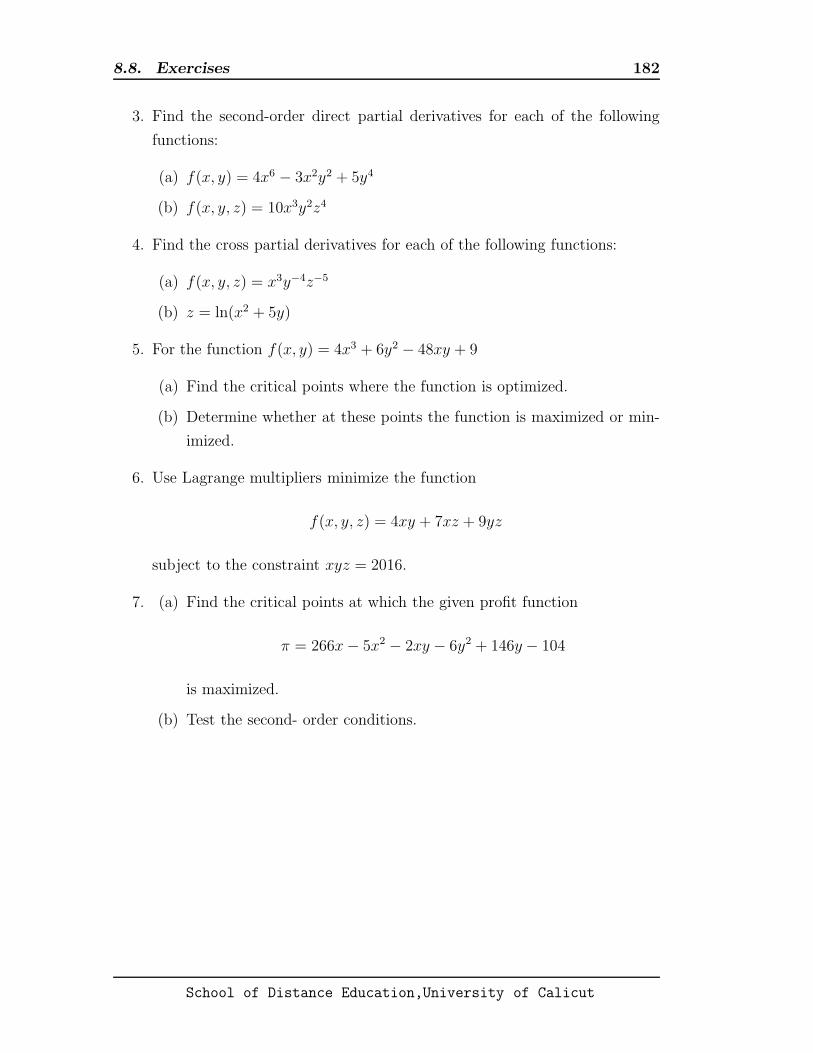
8.8. Exercises 182
3. Find the second-order direct partial derivatives for each of the following
functions:
(a) f(x, y) = 4x6 − 3x2y2 + 5y4
(b) f(x, y, z) = 10x3y2z4
4. Find the cross partial derivatives for each of the following functions:
(a) f(x, y, z) = x3y−4z−5
(b) z = ln(x2 + 5y)
5. For the function f(x, y) = 4x3 + 6y2 − 48xy + 9
(a) Find the critical points where the function is optimized.
(b) Determine whether at these points the function is maximized or min-
imized.
6. Use Lagrange multipliers minimize the function
f(x, y, z) = 4xy + 7xz + 9yz
subject to the constraint xyz = 2016.
7. (a) Find the critical points at which the given profit function
π = 266x− 5x2 − 2xy − 6y2 + 146y − 104
is maximized.
(b) Test the second- order conditions.
School of Distance Education,University of Calicut

Chapter 9More of Integration and Multivariable
Calculus
9.1 Integration by Substitution
Up to this stage, we can do simple integration using formulas and simple rules.
For more complicated ones, like∫
xex2
dx, we have to use some techniques for inte-
gration. In general, different forms of the integrand requires different techniques.
In this section, we discuss a simple but important technique the substitution
method. It is the technique in integration that corresponds to the chain rule in
differentiation
By expressing the integrand f(x) as a function of u and its derivative du/dx,
and integrating with respect to x, we obtain
∫
f(x)dx =
∫(
udu
dx
)
dx
∫
f(x)dx =
∫
udu = F (u) + c
Steps for the Substitution Method
(1) Define a new variable u = g(x), where g(x) is chosen in such a way that
g′(x) “is a factor ” of the integrand and that when written in terms of u,
the integrand is simpler than when written in terms of x.
183

9.1. Integration by Substitution 184
(2) Transform the integral with respect to x into an integral with respect to u
by replacing g(x) everywhere by u and g′(x)dx by du.
(3) Integrate the resulting function of u.
(4) Substitute back u = g(x) to express the result in terms of x.
Problem 9.1. Determine the integral∫
24x3(x4 + 9)dx.
Solution.
(1) Let u = x4 + 9, then du/dx = 4x3 ⇒ dx = du/4x3
(2) Substitute u for x4 + 9 and du/4x3 for dx in the original integrand we get,
∫
24x3(x4 + 9)dx =
∫
24x3 · u · du
4x3=
∫
6udu
(3) Integrate with respect to u we get,
∫
6udu = 6
∫
udu = 6
(
u2
2
)
+ c = 3u2 + c
(4) Replace u by (x4 + 9) we get,
∫
24x3(x4 + 9)dx = 3(x4 + 9)2 + c
�
Problem 9.2. Use integration by substitution to evaluate the indefinite integral
for the following functions:
(a)
∫
56x
(7x2 + 4)3dx
(b)
∫
60x3√5x4 + 9dx
(c)
∫
8xe4x2
dx
(d)
∫
ln x
xdx
School of Distance Education,University of Calicut
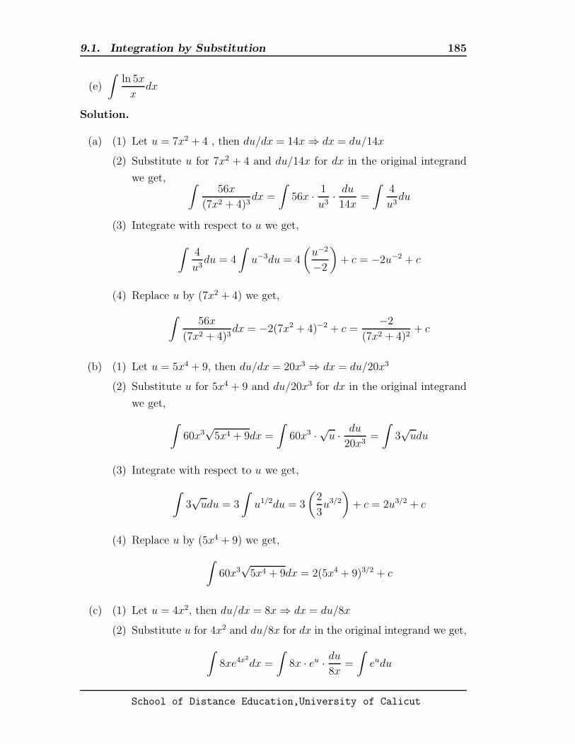
9.1. Integration by Substitution 185
(e)
∫
ln 5x
xdx
Solution.
(a) (1) Let u = 7x2 + 4 , then du/dx = 14x ⇒ dx = du/14x
(2) Substitute u for 7x2 + 4 and du/14x for dx in the original integrand
we get,∫
56x
(7x2 + 4)3dx =
∫
56x · 1
u3· du
14x=
∫
4
u3du
(3) Integrate with respect to u we get,
∫
4
u3du = 4
∫
u−3du = 4
(
u−2
−2
)
+ c = −2u−2 + c
(4) Replace u by (7x2 + 4) we get,
∫
56x
(7x2 + 4)3dx = −2(7x2 + 4)−2 + c =
−2
(7x2 + 4)2+ c
(b) (1) Let u = 5x4 + 9, then du/dx = 20x3 ⇒ dx = du/20x3
(2) Substitute u for 5x4 + 9 and du/20x3 for dx in the original integrand
we get,
∫
60x3√5x4 + 9dx =
∫
60x3 ·√u · du
20x3=
∫
3√udu
(3) Integrate with respect to u we get,
∫
3√udu = 3
∫
u1/2du = 3
(
2
3u3/2
)
+ c = 2u3/2 + c
(4) Replace u by (5x4 + 9) we get,
∫
60x3√5x4 + 9dx = 2(5x4 + 9)3/2 + c
(c) (1) Let u = 4x2, then du/dx = 8x ⇒ dx = du/8x
(2) Substitute u for 4x2 and du/8x for dx in the original integrand we get,
∫
8xe4x2
dx =
∫
8x · eu · du8x
=
∫
eudu
School of Distance Education,University of Calicut

9.1. Integration by Substitution 186
(3) Integrate with respect to u we get,
∫
eudu = eu + c
(4) Replace u by 4x2 we get,
∫
8xe4x2
dx = e4x2
+ c
(d) (1) Let u = ln x, then du/dx =1
x⇒ dx = xdu
(2) Substitute u for ln x and xdu for dx in the original integrand we get,
∫
ln x
xdx =
∫
1
x· u · xdu =
∫
udu
(3) Integrate with respect to u we get,
∫
udu =u2
2+ c
(4) Replace u by ln x we get,
∫
ln x
xdx =
(lnx)2
2+ c =
ln2 x
2+ c
(e) (1) Let u = ln 5x, then du/dx =1
5x· 5 = x ⇒ dx = xdu
(2) Substitute u for ln 5x and xdu for dx in the original integrand we get,
∫
ln 5x
xdx =
∫
1
x· u · xdu =
∫
udu
(3) Integrate with respect to u we get,
∫
udu =u2
2+ c
(4) Replace u by ln x we get,
∫
ln 5x
xdx =
(ln 5x)2
2+ c =
ln2 5x
2+ c
School of Distance Education,University of Calicut

9.2. Integration by Parts 187
9.2 Integration by Parts
The technique in integration that corresponds to the product rule in differenti-
ation is called integration by parts. When an integrand which is a product or
quotient of two differentiable functions of x cannot be expressed as a constant
multiple of udu/dx, integration by parts is frequently helpful.
We have the product rule,
d
dx[f(x) · g(x)] = f(x) · g′(x) + g(x) · f ′(x)
Taking the integral of the derivative we get,
f(x) · g(x) =∫
[f(x) · g′(x)]dx+
∫
[g(x) · f ′(x)]dx
From above equation we get,
∫
[f(x) · g′(x)]dx = f(x) · g(x)−∫
[g(x) · f ′(x)]dx (9.1)
However, to keep things simpler, let us replace f(x) and g(x) with u and v,
respectively. Doing this, we can rewrite the expression as
∫
u
(
dv
dx
)
dx = uv −∫
v
(
du
dx
)
dx
The above equation we can write as
∫
udv = uv −∫
vdu (9.2)
Problem 9.3. Use integration by parts to evaluate the indefinite integral for the
following functions
(a)
∫
9x(x+ 5)2dx
(b)
∫
12x
(x+ 9)5dx
(c)
∫
15x√8 + xdx
School of Distance Education,University of Calicut

9.2. Integration by Parts 188
(d)
∫
(x+ 3)exdx
(e)
∫
x3 ln 2xdx
(f)
∫
ln x4dx
Solution.
(a) In integration by parts the key thing is to choose u and dv correctly.
Let u = 9x and dv = (x + 5)2dx. Then du = 9dx and v =(x+ 5)3
3+ c1
From (9.2),∫
udv = uv −∫
vdu
∫
9x(x+ 5)2dx = uv −∫
vdu
= 9x
[
(x+ 5)3
3+ c1
]
−∫[
(x+ 5)3
3+ c1
]
(9)dx
= 3x(x+ 5)3 + 9c1x−∫
[3(x+ 5)3 + 9c1]dx
= 3x(x+ 5)3 + 9c1x− 3(x+ 5)4
4− 9c1x+ c
= 3x(x+ 5)3 − 3
4(x+ 5)4 + c
Thus we get
∫
9x(x+ 5)2dx = 3x(x+ 5)3 − 3
4(x+ 5)4 + c.
(b) Let u = 12x and dv =1
(x+ 9)5dx = (x + 9)−5dx. Then du = 12dx and
v = −(x+ 9)−4
4+ c1. Substituting in (9.2) we get,
∫
12x
(x+ 9)5dx = uv −
∫
vdu
= 12x
[
−(x+ 9)−4
4+ c1
]
−∫[
−(x+ 9)−4
4+ c1
]
(12)dx
= −3x(x+ 9)−4 + 12c1x−∫
[−3(x+ 9)−4 + 12c1]dx
= −3x(x+ 9)−4 + 12c1x+3(x+ 9)−3
−3− 12c1x+ c
School of Distance Education,University of Calicut
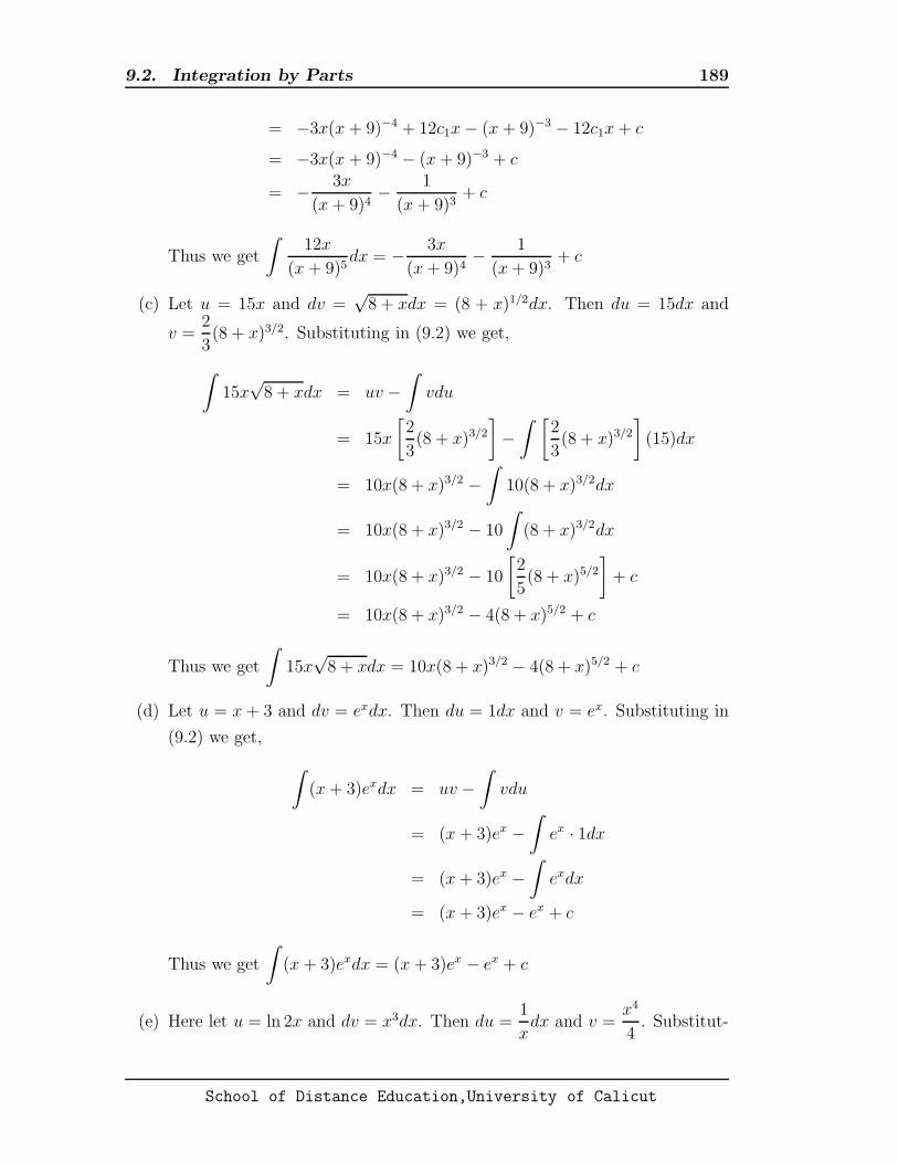
9.2. Integration by Parts 189
= −3x(x + 9)−4 + 12c1x− (x+ 9)−3 − 12c1x+ c
= −3x(x + 9)−4 − (x+ 9)−3 + c
= − 3x
(x+ 9)4− 1
(x+ 9)3+ c
Thus we get
∫
12x
(x+ 9)5dx = − 3x
(x+ 9)4− 1
(x+ 9)3+ c
(c) Let u = 15x and dv =√8 + xdx = (8 + x)1/2dx. Then du = 15dx and
v =2
3(8 + x)3/2. Substituting in (9.2) we get,
∫
15x√8 + xdx = uv −
∫
vdu
= 15x
[
2
3(8 + x)3/2
]
−∫[
2
3(8 + x)3/2
]
(15)dx
= 10x(8 + x)3/2 −∫
10(8 + x)3/2dx
= 10x(8 + x)3/2 − 10
∫
(8 + x)3/2dx
= 10x(8 + x)3/2 − 10
[
2
5(8 + x)5/2
]
+ c
= 10x(8 + x)3/2 − 4(8 + x)5/2 + c
Thus we get
∫
15x√8 + xdx = 10x(8 + x)3/2 − 4(8 + x)5/2 + c
(d) Let u = x+ 3 and dv = exdx. Then du = 1dx and v = ex. Substituting in
(9.2) we get,
∫
(x+ 3)exdx = uv −∫
vdu
= (x+ 3)ex −∫
ex · 1dx
= (x+ 3)ex −∫
exdx
= (x+ 3)ex − ex + c
Thus we get
∫
(x+ 3)exdx = (x+ 3)ex − ex + c
(e) Here let u = ln 2x and dv = x3dx. Then du =1
xdx and v =
x4
4. Substitut-
School of Distance Education,University of Calicut

9.3. Improper Integrals 190
ing in (9.2) we get,
∫
x3 ln 2xdx = uv −∫
vdu
= ln 2x · x4
4−∫
x4
4· 1xdx
=x4
4ln 2x−
∫
x3
4dx
=x4
4ln 2x− 1
4
∫
x3dx
=x4
4ln 2x− 1
4
(
x4
4
)
+ c
=x4
4ln 2x− 1
16x4 + c
Thus we get
∫
x3 ln 2xdx =x4
4ln 2x− 1
16x4 + c
(f) Here let u = ln x4 and dv = 1dx. Then du =1
x4(4x3)dx =
4
xdx and v = x.
Substituting in (9.2) we get,
∫
ln x4dx = uv −∫
vdu
= ln x4 · x−∫
4
x· xdx
= x ln x4 −∫
4dx
= x ln x4 − 4
∫
dx
= x ln x4 − 4x+ c
Thus we get
∫
ln x4dx = x ln x4 − 4x+ c
�
9.3 Improper Integrals
Our original discussion of the definite integral
∫ b
a
f(x)dx assumed that the in-
terval a ≤ x ≤ b was of finite length and that f was continuous. Integrals that
arise in applications don’t necessarily have these nice properties. In this section
School of Distance Education,University of Calicut

9.3. Improper Integrals 191
we investigate a class of integrals, called improper integrals, in which one limit of
integration is infinite. So
∫ ∞
a
f(x)dx,
∫ b
−∞f(x)dx
are improper integrals . Note that
∫ ∞
a
f(x)dx = limb→∞
∫ b
a
f(x)dx
∫ b
∞f(x)dx = lim
a→−∞
∫ b
a
f(x)dx
If the limit in either case exists, the improper integral is said to converge. If the
limit does not exist, the improper integral diverges and meaningless.
Problem 9.4. Evaluate the following improper integrals whenever they are con-
vergent:
(a)
∫ ∞
1
4
x2dx
(b)
∫ ∞
1
5√xdx
(c)
∫ ∞
5
dx
(x− 1)2
(d)
∫ ∞
0
21e−7xdx
Solution.
(a)
∫ ∞
1
4
x2dx = lim
b→∞
∫ b
1
4
x2dx = lim
b→∞
[−4
x
]b
1
= limb→∞
[−4
b−(−4
1
)]
= limb→∞
(−4
b+ 4
)
= 4
School of Distance Education,University of Calicut

9.3. Improper Integrals 192
because b → ∞, (−4/b) → 0. Hence the improper integral is convergent
and∫ ∞
1
4
x2dx = 4
(b)
∫ ∞
1
5√x
= limb→∞
∫ b
1
5√xdx = lim
b→∞
∫ b
1
5x−1/2dx
= limb→∞
[
5x1/2
1/2
]b
1
= limb→∞
[
10x1/2]b
1
= limb→∞
[
10√x]b
1
= limb→∞
[
10√b− 10
]
because b → ∞, (10√b − 10) increases without bound. So the integral has
no limit and is divergent.
(c)
∫ ∞
5
dx
(x− 1)2= lim
b→∞
∫ b
5
dx
(x− 1)2= lim
b→∞
∫ b
5
(x− 1)−2dx
= limb→∞
[
(x− 1)−1
−1
]b
5
= limb→∞
[ −1
(x− 1)
]b
5
= limb→∞
[ −1
(b− 1)+
1
4
]
= limb→∞
[ −1
(b− 1)
]
+ limb→∞
1
4
=1
4
because b → ∞,−1/(b−1) → 0. Hence the improper integral is convergent
and∫ ∞
5
dx
(x− 1)2=
1
4
School of Distance Education,University of Calicut

9.3. Improper Integrals 193
(d)
∫ ∞
0
21e−7xdx = limb→∞
∫ b
0
21e−7xdx
= limb→∞
[
21e−7x
−7
]b
0
= limb→∞
[
−3e−7x]b
0
= limb→∞
[
−3e−7b + 3e−7(0)]
= limb→∞
[
−3e−7b + 3]
= 3
because b → ∞,−3e−7b → 0. Hence the improper integral is convergent
and∫ ∞
0
21e−7xdx = 3
�
Problem 9.5. Evaluate the following improper integrals whenever they are con-
vergent:
(a)
∫ ∞
1
8
xdx
(b)
∫ 0
−∞28e4xdx
Solution.
(a)
∫ ∞
1
8
xdx = lim
b→∞
∫ b
1
8
xdx
= limb→∞
[8 lnx]b1
= limb→∞
[8 ln b− 8 ln 1]
= limb→∞
(8 ln b) Since ln 1 = 0
As b → ∞, 8 ln b → ∞, so the improper integral diverges and has no definite
value.
School of Distance Education,University of Calicut

9.4. L’Hopital’s Rule 194
(b)
∫ 0
−∞28e4xdx = lim
b→−∞
∫ 0
b
28e4xdx
= limb→−∞
[
28e4x
4
]0
b
= limb→−∞
[7e4x]0b
= limb→−∞
[7e4(0) − 7e4b]
= limb→−∞
[7− 7e4b] = 7
because b → −∞,−7e4b → 0. Hence the improper integral is convergent
and∫ 0
−∞28e4xdx = 7
�
9.4 L’Hopital’s Rule
We use L’hopital’s rule if the limit of a function f(x) = g(x)/h(x) as x → a can
not be evaluated, such as (1) when both numerator and denominator approach
zero, giving rise to the indeterminate form 00or (2) when both numerator and
denominator approach infinity, giving rise to the indeterminate form ∞/∞.
L’hopital’s rule states that
limx→a
g(x)
h(x)= lim
x→a
g′(x)
h′(x)(9.3)
Problem 9.6. Use L’hopital’s rule to evaluate the following limits:
(a) limx→3
x− 3
9− x2
(b) limx→∞
5x2 − 2x
3x2 + 3x
(c) limx→∞
x− 7
ex
(d) limx→∞
1− e1/x
1/x
School of Distance Education,University of Calicut
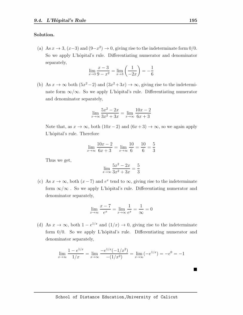
9.4. L’Hopital’s Rule 195
Solution.
(a) As x → 3, (x−3) and (9−x2) → 0, giving rise to the indeterminate form 0/0.
So we apply L’hopital’s rule. Differentiating numerator and denominator
separately,
limx→3
x− 3
9− x2= lim
x→3
(
1
−2x
)
= −1
6
(b) As x → ∞ both (5x2−2) and (3x2+3x) → ∞, giving rise to the indetermi-
nate form ∞/∞. So we apply L’hopital’s rule. Differentiating numerator
and denominator separately,
limx→∞
5x2 − 2x
3x2 + 3x= lim
x→∞
10x− 2
6x+ 3
Note that, as x → ∞, both (10x− 2) and (6x+3) → ∞, so we again apply
L’hopital’s rule. Therefore
limx→∞
10x− 2
6x+ 3= lim
x→∞
10
6=
10
6=
5
3
Thus we get,
limx→∞
5x2 − 2x
3x2 + 3x=
5
3
(c) As x → ∞, both (x−7) and ex tend to ∞, giving rise to the indeterminate
form ∞/∞ . So we apply L’hopital’s rule. Differentiating numerator and
denominator separately,
limx→∞
x− 7
ex= lim
x→∞
1
ex=
1
∞ = 0
(d) As x → ∞, both 1 − e1/x and (1/x) → 0, giving rise to the indeterminate
form 0/0. So we apply L’hopital’s rule. Differentiating numerator and
denominator separately,
limx→∞
1− e1/x
1/x= lim
x→∞
−e1/x(−1/x2)
−(1/x2)= lim
x→∞(−e1/x) = −e0 = −1
�
School of Distance Education,University of Calicut

9.5. Double Integrals 196
9.5 Double Integrals
If z = f(x, y) and R1 is the region in the xy plane bounded by y = g(x) and
y = h(x) between x = a and x = b. Then the volume of the solid bounded by
f(x, y) over the region R1 is defined by the double or iterated integral
∫ ∫
R1
f(x, y)dydx =
∫ b
a
[
∫ h(x)
g(x)
f(x, y)dy
]
dx (9.4)
If z = f(x, y) and R2 is the region in the xy plane bounded by y = c and y = d
between x = g(y) and x = h(y). Then the volume of the solid bounded by f(x, y)
over the region R2 is
∫ ∫
R2
f(x, y)dxdy =
∫ d
c
[
∫ h(y)
g(y)
f(x, y)dx
]
dy (9.5)
To compute a double integral such as (9.4), we first compute the inner definite
integral∫ h(x)
g(x)
f(x, y)dy
taking the antiderivative of f with respect to y by treating x as a constant. This
result in a function of x alone which we then simply integrate over the limits x = a
to x = b. The procedure for the double integral in (9.5) is perfectly analogous.
Problem 9.7. Calculate the following double integrals:
(a)
∫ 2
1
∫ 3
2
(6x+ 2y)dydx
(b)
∫ 1
0
∫ 2
1
60x2y3dydx
(c)
∫ 1
0
∫
√x
x
240xy3dydx
(d)
∫ 2
1
∫ 3y
y
12xydxdy
School of Distance Education,University of Calicut
9.5. Double Integrals 197
Solution.
(a) Note that,
∫ 2
1
∫ 3
2
(6x+ 2y)dydx =
∫ 2
1
(∫ 3
2
(6x+ 2y)dy
)
dx
Computing the inner integration with respect to y while holding x constant,
∫ 2
1
∫ 3
2
(6x+ 2y)dydx =
∫ 2
1
[∫ 3
2
(6xy + y2)∣
∣
y=3
y=2
]
dx
=
∫ 2
1
[(18x+ 9)− (12x+ 4)] dx
=
∫ 2
1
(6x+ 5)dx
= (3x2 + 5x)∣
∣
2
1
= (12 + 10)− (3 + 5) = 14
So,∫ 2
1
∫ 3
2
(6x+ 2y)dydx = 14
(b) Note that,∫ 1
0
∫ 2
1
60x2y3dydx =
∫ 1
0
(∫ 2
1
60x2y3dy
)
dx
Computing the inner integration with respect to y while holding x constant,
∫ 1
0
∫ 2
1
60x2y3dydx =
∫ 1
0
[∫ 2
1
(15x2y4)∣
∣
y=2
y=1
]
dx
=
∫ 1
0
(240x2 − 15x2)dx
=
∫ 1
0
225x2dx
= 75x3∣
∣
1
0= 75
So,
∫ 1
0
∫ 2
1
60x2y3dydx = 75.
School of Distance Education,University of Calicut
9.5. Double Integrals 198
(c) Note that,
∫ 1
0
∫
√x
x
240xy3dydx =
∫ 1
0
(
∫
√x
x
240xy3dy
)
dx
Computing the inner integration with respect to y while holding x constant,
∫ 1
0
∫
√x
x
240xy3dydx =
∫ 1
0
[
(60xy4)∣
∣
y=√x
y=x
]
dx
=
∫ 1
0
[60x(√x)4 − 60x(x)4]dx
=
∫ 1
0
(60x3 − 60x5)dx
= (15x4 − 10x6)∣
∣
1
0
= (15− 10)− (0− 0) = 5
(d) Note that,∫ 2
1
∫ 3y
y
12xydxdy =
∫ 2
1
(∫ 3y
y
12xydx
)
dy
Computing the inner integration with respect to x while holding y constant,
∫ 2
1
∫ 3y
y
12xydxdy =
∫ 2
1
[
(6x2y)∣
∣
x=3y
x=y
]
dy
=
∫ 1
0
[6(3y)2y − 6(y)2y]dy
=
∫ 2
1
(54y3 − 6y3)dy
=
∫ 2
1
48y3dy
= (12y4)∣
∣
2
1
= 12(2)4 − 12 = 192− 12 = 180
So the value of the double integral
∫ 2
1
∫ 3y
y
12xydxdy is 180.
�
School of Distance Education,University of Calicut

9.6. Approximating Definite Integrals 199
9.6 Approximating Definite Integrals
Given an interval a ≤ x ≤ b divided in to n equal subintervals, each of length
∆x = (b − a)/n, in which the end points of the subintervals are denoted by
g0, g1, . . . gn and the midpoints by h1, h2, . . . hn we have,
Rectangular Rule
∫ b
a
f(x)dx ≈ f(h1)∆x+ f(h1)∆x+ · · ·+ f(hn−1)∆x+ f(hn)∆x
= [f(h1) + f(h2) + · · ·+ f(hn−1) + f(hn)]∆x (9.6)
Trapezoidal Rule
∫ b
a
f(x)dx ≈ [f(g0) + 2f(g1) + 2f(g2) + · · ·+ 2f(gn−1) + f(gn)]∆x
2(9.7)
Simpson’s Rule
∫ b
a
f(x)dx ≈ [f(g0) + 4f(h1) + 2f(g1) + 4f(h2) + 2f(g2) + 4f(h3)
+2f(g3) + · · ·+ 2f(gn−1) + 4f(hn) + f(gn)]∆x
6(9.8)
Problem 9.8. Approximate the value of the definite integral
∫ 8
6
(x− 3)2dx with
the (1) Rectangle Rule, (2) Trapezoidal rule, (3) Simpson’s rule for n = 5. Also
check the accuracy of the answers by using integration.
Solution. (1) The given interval is [6, 8] and n = 5 , So
∆x =b− a
n=
8− 6
5=
2
5= 0.4
So the midpoints hi are 6.2, 6.6 , 7.0, 7.4 and 7.8
Taking the Rectangle rule from (9.6) and substituting,
∫ b
a
f(x)dx ≈ [f(h1) + f(h2) + · · ·+ f(hn−1) + f(hn)]∆x
School of Distance Education,University of Calicut

9.6. Approximating Definite Integrals 200
∫ 8
6
(x− 3)2dx ≈ [f(6.2) + f(6.6) + f(7.0) + f(7.4) + f(7.8)]∆x
≈ [(6.2− 3)2 + (6.6− 3)2 + (7− 3)2 + (7.4− 3)2 + (7.8− 3)2](0.4)
≈ [(3.2)2 + (3.6)2 + (4)2 + (4.4)2 + (4.8)2](0.4)
≈ (10.24 + 12.96 + 16 + 19.36 + 23.04)(0.4)
≈ 32.64
(2) The end points gi are 6, 6.4 , 6.8, 7.2, 7.6 and 8.0
Taking the Trapezoidal rule from (9.7) and substituting,
∫ b
a
f(x)dx ≈ [f(g0) + 2f(g1) + · · ·+ 2f(gn−1) + f(gn)]∆x
2
∫ 8
6
(x− 3)2dx ≈ [f(6) + 2f(6.4) + 2f(6.8) + 2f(7.2) + 2f(7.6) + f(8)](0.4)
2
≈ [(6− 3)2 + 2(6.4− 3)2 + 2(6.8− 3)2 + 2(7.2− 3)2
+2(7.6− 3)2 + (8− 3)2](0.2)
≈ [(3)2 + 2(3.4)2 + 2(3.8)2 + 2(4.2)2 + 2(4.6)2 + (5)2](0.2)
≈ (9 + 23.12 + 28.88 + 35.28 + 42.32 + 25)(0.2)
≈ 32.72
(3) Taking the Simpson’s rule from (9.8) and substituting,
∫ b
a
f(x)dx ≈ [f(g0) + 4f(h1) + 2f(g1) + 4f(h2) + 2f(g2) + 4f(h3)
+2f(g3) + · · ·+ 2f(gn−1) + 4f(hn) + f(gn)]∆x
6∫ 8
6
(x− 3)2dx ≈ [f(6) + 4f(6.2) + 2f(6.4) + 4f(6.6) + 2f(6.8) + 4f(7) + 2f(7.2)
4f(7.4) + 2f(7.6) + 4f(7.8) + f(8)]0.4
6
≈ [(6− 3)2 + 4(6.2− 3)2 + 2(6.4− 3)2 + 4(6.6− 3)2 + 2(6.8− 3)2
+4(7− 3)2 + 2(7.2− 3)2 + 4(7.4− 3)2 + 2(7.6− 3)2 + 4(7.8− 3)2
+(8− 3)2](0.0667)
School of Distance Education,University of Calicut

9.7. Differential Equations 201
≈ [(3)2 + 4(3.2)2 + 2(3.4)2 + 4(3.6)2 + 2(3.8)2 + 4(4)2 + 2(4.2)2
+4(4.4)2 + 2(4.6)2 + 4(4.8)2 + (5)2](0.0667)
≈ 32.683
Calculating the definite integral for comparison,
∫ 8
6
(x− 3)2dx =
[
(x− 3)3
3
]8
6
=1
3[53 − 33] = 32.6667
�
9.7 Differential Equations
A differential equation is an equation expressing a relationship between a function
y = f(t) and one or more of its derivatives.
Example 9.1. Following are some examples of differential equations:
(1)dy
dt= 2t2 + 5
(2) y′ = 6y
(3) y′′ − 3y′ + 5 = 0
The solution of a differential equation is any function, without derivative or
differential, which is defined over an interval and satisfies the differential equation
for all t in the interval.
Example 9.2. To solve the differential equation dy/dt = 8t+ 5 for all the func-
tions y(t) which satisfy the equation, simply integrate both sides to find the
antiderivatives.∫
dy
dtdt =
∫
(8t+ 5)dt
y + c1 = 4t2 + 5t+ c2
y = 4t2 + 5t+ c where c = c2 − c1
This is called a general solution, indicating that when c is unspecified, a
differential equation has an infinite number of possible solutions. If c can be
specified, we have a particular solution and it alone of all the possible solutions
is relevant.
School of Distance Education,University of Calicut
9.7. Differential Equations 202
Example 9.3. A frequently encountered differential equation is one in which the
derivative is expressed as a constant multiple of the function itself;
y′ = ky
This type of differential equation cannot be solved with the method above. Re-
calling, however, that given
y = Aekt y′ = k ·Aekt
By substituting y for Aekt in y′, we have
y′ = ky
Hence a solution for an equation in the familiar form y′ = ky is
y = Aekt A, k constants.
Problem 9.9. Find (1) the general and (2) the particular solution for each of
the following differential equations:
(a) y′(t) = 9t2 − 14t+ 34, y(0) = 5
(b)dy
dt= 20(t− 6)3, y(7) = 8
Solution .
(a) (1) Integrate both sides, ignoring the constant of integration until final step.
∫
y′(t)dt =
∫
(9t2 − 14t+ 34)dt
y = 9 · t3
3− 14 · t
2
2+ 34t+ c
y = 3t3 − 7t2 + 34t+ c
(2) Given y(0) = 5. This condition is known as initial condition. y(0) = 5
means at t = 0, y = 5. Substitute this in the general solution we get,
5 = 3(0)3 − 7(0)2 + 34(0) + c ⇒ c = 5
School of Distance Education,University of Calicut

9.8. Separation of Variables 203
So the solution (particular solution ) is y = 3t3 − 7t2 + 34t+ 5
(b) (1) Integrate both sides,
∫
dy
dtdt =
∫
20(t− 6)3dt
y = 20 · (t− 6)4
4+ c
y = 5(t− 6)4 + c
(2) Using the information y(7) = 8, called a boundary condition whenever
the value of y is given at a point other than t = 0,
8 = 5(7− 6)4 + c = 5 + c ⇒ c = 3
So the solution (particular solution ) is y = 5(t− 6)4 + 3
�
9.8 Separation of Variables
A differential equation in the form
dy
dt=
f(t)
g(y)(9.9)
is separable if it can be rearranged by multiplication so that all terms with y
including dy are on one side of the equal sign and all terms with t including dt
are on the other, such as
g(y)dy = f(t)dt
where g(y) is a function of y alone and f(t) is a function of t alone. A solution
for such an equation is then obtainable by simply integrating each side of the
equation with respect to its individual variable:
∫
g(y)dy =
∫
f(t)dt
School of Distance Education,University of Calicut
9.8. Separation of Variables 204
Problem 9.10. Find the general solution for each of the following differential
equations by separating the variables:
(a)dy
dt=
15t2
4y3
(b) 2ydy
dt= 6t2
(c) y′ = t2e3y
Solution.
(a) (1) Treating dy/dt as a ratio of differentials, separate the variables (by
multiplying both sides of the equation by 4y3dt ), integrate and solve alge-
braically for y,
∫
4y3dy =
∫
15t2dt
4 · y4
4+ c1 = 15 · t
3
3+ c2
y4 + c1 = 5t3 + c2
y4 = 5t3 + c where c = c2 − c1
y = ± 4√5t3 + c
(2) Check the answer by differentiating and substituting.
dy
dt=
d
dt(5t3 + c)1/4 =
1
4(5t3 + c)−3/4 · 15t2
=15t2
4· 1
(5t3 + c)3/4
=15t2
4· 1
[(5t3 + c)1/4]3
=15t2
4· 1
y3
=15t2
4y3
(b) The given differential equation is 2ydy
dt= 6t2, by separating variables we
get,
2ydy = 6t2dt
School of Distance Education,University of Calicut

9.9. Practical Applications 205
Integrating both sides we get,
∫
2ydy =
∫
6t2dt
y2 = 2t3 + c
y = ±√2t3 + c
(c) The given differential equation isdy
dt= t2e3y, by separating variables we
get,dy
e3y= t2dt
Integrating both sides we get,
∫
dy
e3y=
∫
t2dt∫
e−3ydy =
∫
t2dt
e−3y
−3=
t3
3+ c
e−3y = −t3 + k where k = −3c
Take natural logarithm on both sides ( recall ln ef(x) = f(x) ) we get,
−3y = ln(−t3 + k)
y = −1
3ln(k − t3)
�
9.9 Practical Applications
Integral calculus and differential equations are used in business and all the sci-
ences. Integration is used to evaluate the present value of cash flows, for instance;
differential equations to study various forms of population growth under different
circumstances.
Example 9.4. If the present value P under continuous compounding of a sum
of money to be received in the future is P = Ae−rt, the present value of a cash
flow (money to be received each year for n years) is given by the integral
School of Distance Education,University of Calicut

9.9. Practical Applications 206
Pn =
∫ n
0
Ae−rtdt = A
∫ n
0
e−rtdt
= A
[
−e−rt
r
]n
0
= −A
r
[
e−rt]n
0
= −A
r(e−rn − e−r(0)) = −A
r(e−rn − 1)
=A
r(1− e−rn)
∴ Pn =A
r(1− e−rn) (9.10)
Example 9.5. The growth of populations facing factors that inhibit growth over
time, such as the scarcity of food or water, is given by the differential equation,
called a limited growth function
dy
dt= k(M − y) (9.11)
where M is the maximum population size, y is the current population size, and
k is the growth rate.
Problem 9.11. Find the present value of $ 5,000 to be paid each year for 4 years
when the interest rate is 8% compounded continuously
Solution. From (9.10) we have,
Pn =A
r(1− e−rn)
Here A = 5, 000, r = 8% = 0.08, t = 4 . Substituting in above equation we get,
Pn =5, 000
0.08(1− e−(0.08)(4))
= 62, 500(1− e−0.32)
= 62, 500(1− 0.72615)
= 17, 115.63
�
School of Distance Education,University of Calicut

9.9. Practical Applications 207
Problem 9.12. A hive which can support a maximum of 7000 bees currently
has 5000 growing exponentially at a constant rate of 5% a year . What will the
population be in 4 years ?
Solution. Comparing with (9.11) we get M = 7000, k = 5% = 0.05
Substituting in (9.11) we get,
dy
dt= 0.05(7000− y)
Separate the variables and integrate,
∫
dy
7000− y=
∫
0.05dt
− ln(7000− y) = 0.05t+ c
ln(7000− y) = −0.05t− c
7000− y = e−0.05t−c
7000− y = e−0.05t · e−c
7000− y = Ae−0.05t (where A = e−c)
−y = Ae−0.05t − 7000
y = 7000− Ae−0.05t
Thus we get,
y = 7000−Ae−0.05t. (9.12)
Substituting y(0) = 5000 in (9.12) we get,
5000 = 7000− Ae−0.05(0) = 7000− A ⇒ A = 2000
Thus y = 7000− 2000e−0.05(4) = 7000− 2000(0.81873) ≈ 5363. �
School of Distance Education,University of Calicut

9.10. Exercises 208
9.10 Exercises
1. Use integration by substitution to evaluate the indefinite integral for the
following functions:
(a)
∫
3x2(x3 + 7)5dx
(b)
∫
128x(8x2 − 9)3dx
(c)
∫
7x2x
(7x3 − 6)3dx
(d)
∫
10x+ 3
(5x2 + 3x− 7)4dx
(e)
∫
66x3√8x2 − 15dx
2. Use integration by substitution to evaluate the indefinite integral for the
following functions:
(a)
∫
80x3e5x4
dx
(b)
∫
x4ex5
dx
(c)
∫
(1− x2)e3x−x3
dx
(d)
∫
(ln x)2
xdx
(e)
∫
1
x(ln 7x)3dx
3. Use integration by parts to evaluate the indefinite integral for the following
functions:
(a)
∫
x(x− 6)4dx
(b)
∫
8x
(x− 5)2dx
(c)
∫
6x√x+ 7
dx
(d)
∫
7x
ex+5dx
(e)
∫
5x+ 2
exdx
School of Distance Education,University of Calicut
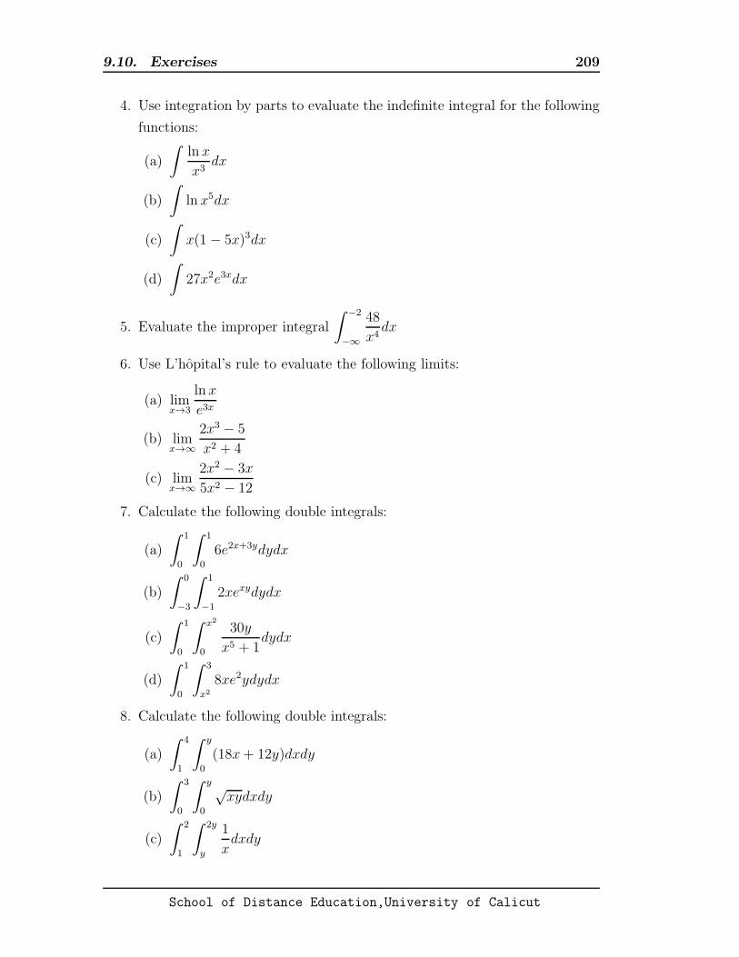
9.10. Exercises 209
4. Use integration by parts to evaluate the indefinite integral for the following
functions:
(a)
∫
ln x
x3dx
(b)
∫
ln x5dx
(c)
∫
x(1 − 5x)3dx
(d)
∫
27x2e3xdx
5. Evaluate the improper integral
∫ −2
−∞
48
x4dx
6. Use L’hopital’s rule to evaluate the following limits:
(a) limx→3
ln x
e3x
(b) limx→∞
2x3 − 5
x2 + 4
(c) limx→∞
2x2 − 3x
5x2 − 12
7. Calculate the following double integrals:
(a)
∫ 1
0
∫ 1
0
6e2x+3ydydx
(b)
∫ 0
−3
∫ 1
−1
2xexydydx
(c)
∫ 1
0
∫ x2
0
30y
x5 + 1dydx
(d)
∫ 1
0
∫ 3
x2
8xe2ydydx
8. Calculate the following double integrals:
(a)
∫ 4
1
∫ y
0
(18x+ 12y)dxdy
(b)
∫ 3
0
∫ y
0
√xydxdy
(c)
∫ 2
1
∫ 2y
y
1
xdxdy
School of Distance Education,University of Calicut

9.10. Exercises 210
9. Approximate the value of the definite integral
∫ 1
−1
e3xdx with the (1) Rect-
angle Rule, (2) Trapezoidal rule, (3) Simpson’s rule for n = 4. Also check
the accuracy of the answers by using integration.
10. Approximate the value of the definite integral
∫ 2.4
1.2
xexdx with the (1) Rect-
angle Rule, (2) Trapezoidal rule, (3) Simpson’s rule for n = 3. Also check
the accuracy of the answers by using integration.
11. Find (1) the general and (2) the particular solution for each of the following
differential equations:
(a) y′(t) = 18e3t − 8e2t + 9, y(0) = −3
(b) 3dy
dt= 63
√t− 12, y(12) = 7
(c) y′(t) = −3y, y(0) = 14
(d) y′(t) = −0.25y, y(0) = 8
12. Find the general solution for each of the following differential equations by
separating the variables:
(a)dy
dt= t4y2
(b) y′ = et−y
(c) y′ = 4t3y − 3t2y
13. The rate at which the number of insects decreases after t hours following
the introduction of a pesticide is given by
dy
dt=
−540
1 + 3t
If there are 1000 insects initially, find their number at t = 5.
School of Distance Education,University of Calicut

9.10. Exercises 211
Text Books (As per Syllabus)
Edward T. Dowling: Calculus for Business, Economics and Social
Sciences, Schaum’s Outline Series, TMH, 2005.
Further Readings
1. Ismor Fischer: Basic Calculus Refresher,
http://www.stat.wisc.edu/ ifischer/calculus.pdf
2. S.K Chung: Understanding Basic Calculus,
http://www.mathdb.org/basic−calculus/BasicCalculus.pdf
3. Srinath Baruah : Basic Mathematics and its Applications in Economics,
Macmillan.
4. Taro Yamane: Mathematics for Economists, Second ed., PHI.
———————————————————————————————
School of Distance Education,University of Calicut