
Shannon Wang, M.A., CCC-SLP Nancy Castilleja, M.A., CCC-SLP Marie Sepulveda, M.S., CCC-SLP

CCC Enrollment Projection: A Statewide Model
For the 2009 CAIR Conference, Sacramento, CA
November 18‐20, 2009
1

Your Speakers
• Mei CoocSpecialist: Information Systems & Analysis
Research & Planning Unit
California Community Colleges Chancellor’s Office
• Willard HomDirector
Research & Planning Unit
California Community Colleges Chancellor’s Office
2
Objectives of the Session
• Present some recent efforts at the Chancellor’s Office to expand our planning
and policy‐making knowledge base regarding system enrollment
• Obtain feedback and/or suggestions from other practitioners and theorists
3
Objectives of the Analysis
• Develop a statewide model (because we currently run only district‐level projections)
• Explore variables that explain enrollment
• Project Hispanic enrollment
4

Specific Projection Purposes—1
• How many students should the CCC system expect to enroll in
a specific period in the future?
Funding needs
Facility needs
Instructional resources
Educational pipeline volume
5

Specific Projection Purposes—2
• How many Hispanic students should the CCC system expect to
enroll in a specific period in the future?
Educational pipeline volume
Educational opportunity
6

Data Limitations
• Total statewide enrollment headcounts (1975‐ 2007)
– Paper submission vs. electronic submission (1992)
• Hispanic enrollment headcounts (1992‐2007)
• DOF Adult Population Projections (1992‐1999)& Estimates (2000‐2007)
7
Layout of the Presentation
Part I: Total Statewide projection model
Part II: Hispanic projection model
8
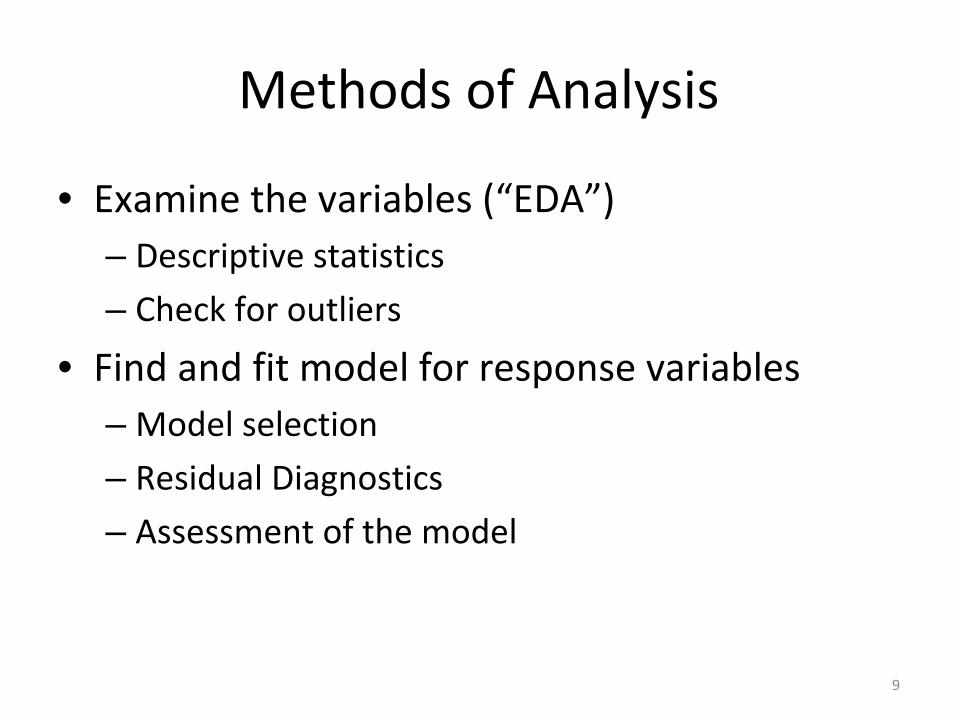
Methods of Analysis
• Examine the variables (“EDA”)– Descriptive statistics– Check for outliers
• Find and fit model for response variables– Model selection
– Residual Diagnostics– Assessment of the model
9
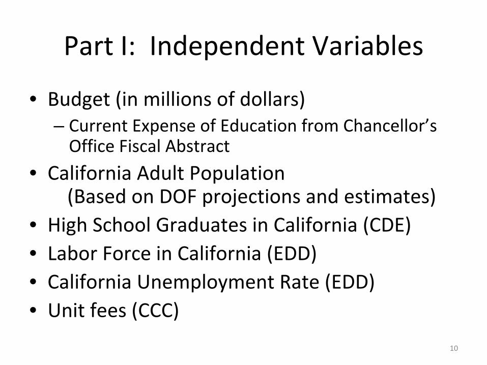
Part I: Independent Variables
• Budget (in millions of dollars)– Current Expense of Education from Chancellor’s
Office Fiscal Abstract
• California Adult Population (Based on DOF projections and estimates)
• High School Graduates in California (CDE)• Labor Force in California (EDD)• California Unemployment Rate (EDD)• Unit fees (CCC)
10
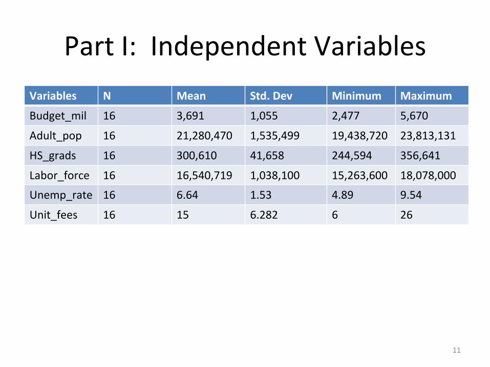
Part I: Independent Variables
Variables N Mean Std. Dev Minimum Maximum
Budget_mil 16 3,691 1,055 2,477 5,670
Adult_pop 16 21,280,470 1,535,499 19,438,720 23,813,131
HS_grads 16 300,610 41,658 244,594 356,641
Labor_force 16 16,540,719 1,038,100 15,263,600 18,078,000
Unemp_rate 16 6.64 1.53 4.89 9.54
Unit_fees 16 15 6.282 6 26
11

Part I: Dependent Variables• Total statewide enrollment headcount
Variable N Mean Std. Dev Minimum Maximum
Fall_enrollment 16 1,544,221 131,495 1,336,202 1,747,930
12

Part I: Model Selection
Model (Fall Enrollment = …) #of Variables Adj. R2
‐905,008.4 + 0.157 labor_force
–
9,804.807 unit_fees 2 0.952
‐858,574+ 0.124 adult_pop –
15,815.031 unit_fees 2 0.943
469,742 + 4.229 HS_grads
–
13,115.01 unit_fees 2 0.912
1,126,964 + 165.807 budget_mil –
12,979.6 unit_fees 2 0.898
‐378,567.7 + 0.116 labor_force 1 0.831
720,588.46 + 2.74 HS_grads 1 0.736
1,147,075 + 107.606 budget_mil 1 0.727
43,319.911 + 0.070 adult_pop 1 0.715
1,922,317 + ‐56,958.3 unemp_rate 1 0.398
13

Part I: Residual Analysis for Model 1
• Autocorrelation: Durbin‐Watson 1.813
• Normality of error terms assumption:– Shapiro Wilk’s test: p‐value = 0.776
• Constant variance (Homoscedasticity)
14
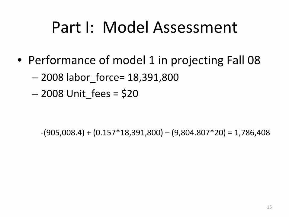
Part I: Model Assessment
• Performance of model 1 in projecting Fall 08– 2008 labor_force= 18,391,800– 2008 Unit_fees = $20
‐(905,008.4) + (0.157*18,391,800) –
(9,804.807*20) = 1,786,408
15

Are We in the Ballpark?
• 95% prediction interval: – Lower Bound = 1,714,768
Upper Bound = 1,856,733
• Actual Fall 2008 Total Enrollment: 1,824,624
16
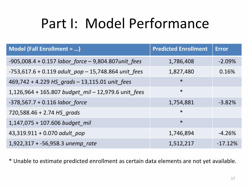
Part I: Model Performance
Model (Fall Enrollment = …) Predicted Enrollment Error
‐905,008.4 + 0.157 labor_force –
9,804.807unit_fees 1,786,408 ‐2.09%
‐753,617.6 + 0.119 adult_pop
–
15,748.864 unit_fees 1,827,480 0.16%
469,742 + 4.229 HS_grads
–
13,115.01 unit_fees *
1,126,964 + 165.807 budget_mil
–
12,979.6 unit_fees *
‐378,567.7 + 0.116 labor_force 1,754,881 ‐3.82%
720,588.46 + 2.74 HS_grads *
1,147,075 + 107.606 budget_mil *
43,319.911 + 0.070 adult_pop 1,746,894 ‐4.26%
1,922,317 + ‐56,958.3 unemp_rate 1,512,217 ‐17.12%
* Unable to estimate predicted enrollment as certain data elements are not yet available.
17
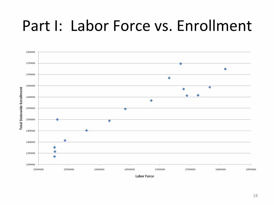
Part I: Labor Force vs. Enrollment
18

Part I: Labor Force vs. Enrollment20022001
19
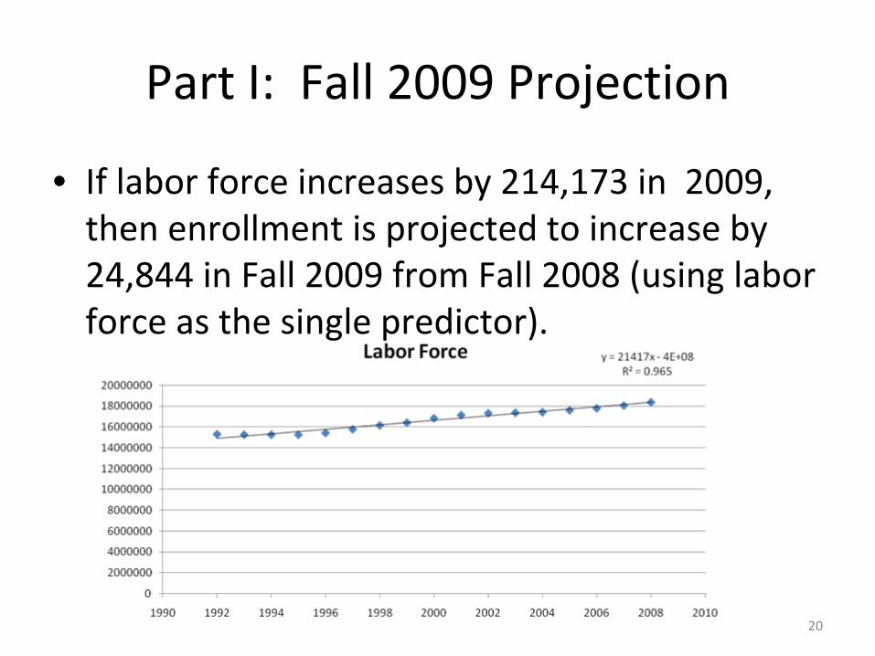
Part I: Fall 2009 Projection
• If labor force increases by 214,173 in 2009, then enrollment is projected to increase by 24,844 in Fall 2009 from Fall 2008 (using labor
force as the single predictor).
20
Part II: Hispanic Enrollment Projection
21

Part II: Independent Variables
• Budget (in millions of dollars)– Current Expense of Education from Chancellor’s Office
Fiscal Abstract
• Hispanic Adult Population in California(based on DOF projections and estimates)
• High School Graduates in California (CDE)• Labor Force in California (EDD)• Unemployment Rate in California (EDD)• Unit fees (CCC)
22

Part II: Dependent Variable
• Fall Hispanic enrollment headcount
23

Part II: Variables
Independent Variables N Mean Std. Dev Minimum Maximum
Budget_mil 16 3,691 1,055 2,477 5,670
Hisp_pop 16 6,249,379 1,230,458 4,621,658 8,259,420
HS_grads 16 300,610 41,658 244,594 356,641
Labor_force 16 16,540,719 1,038,100 15,263,600 18,078,000
Unemp_rate 16 6.6381 1.52856 4.89 9.54
Unit_fees 16 15 6.282 6 26
Dependent Variable N Mean Std. Dev Minimum Maximum
Fall Hispanic Enrollment 16 396,568 76,654 291,725 516,733
24

Part II: Model Selection
Model (Fall Hispanic Enrollment = …) #of Variables R2 Adj. R2
‐16,035.7+ 0.074 hisp_pop –
3,324.586 unit_fees 2 0.985 0.982
‐854,782 + 0.076 labor_force –
770.47 unit_fees 2 0.984 0.981
‐813,414 + 0.073 labor_force 1 0.981 0.980
674.395 + 0.064 hisp_pop 1 0.955 0.952
‐142,469 + 1.793 HS_grads 1 0.950 0.946
136,251.4 + 70.532 budget_mil 1 0.943 0.939
654,698.8 –
38,886.1 unemp_rate 1 0.601 0.573
278,255.1 + 7,887.519 unit_fees 1 0.418 0.376
25

Part II: Model 1
26

Part II: Residual Analysis for Model 1
• Autocorrelation: Durbin‐Watson = 1.622
• Normality of error terms assumption:– Shapiro Wilk’s test: p‐value = 0.756
• Constant variance (Homoscedasticity)
27

Part II: Model Assessment
• Performance of model 1 in projecting Fall 08 Hispanic enrollment
– 2008 Hispanic Adult Population = 8,294,366– 2008 Unit_fees = $20
• ‐16,035.7 + 0.074 *8,294,366 –
3,324.586 *20 = 531,256
28

Again, are we in the ballpark?
• 95% prediction interval:– Lower Bound = 480,650
Upper Bound = 561,453
• Actual Fall 2008 Hispanic Headcount = 553,777
29

Part II: Model Performance
Model (Fall Hispanic Enrollment = …) Predicted Enrollment Error
‐16,035.7+ 0.074 hisp_pop –
3,324.586 unit_fees 531,256 ‐4.07%
‐854,782 + 0.076 labor_force –
770.47 unit_fees 527,585 ‐4.73%
‐813,414 + 0.073 labor_force 529,157 ‐4.45%
674.395 + 0.064 hisp_pop 531,514 ‐4.02%
‐142,469 + 1.793 HS_grads *
136,251.4 + 70.532 budget_mil *
654,698.8 –
38,886.1 unemp_rate 374,719 ‐32.33%
278,255.1 + 7,887.519 unit_fees 436,005 ‐21.27%
* Unable to estimate predicted enrollment as certain data elements are not yet available.
30
Potential Model Enhancements
• Hispanic labor force as a predictor• Number of Hispanic high school graduates
• Estimates of adult population instead of projections
31

A Quotation
• “No one factor determines enrollments at a college or university.”
(Brinkman & McIntyre, 1997, p. 67)
32
Interpretation—Part 1
• Unit fee level is more volatile in nature than labor force.
• Although the enrollment fee can be “manipulated,”
our simple model does not imply
that an abrupt shift or shock to fee level would cause a response in state enrollment levels.
• If we predicted fee levels on the basis of a model, then that prediction of new fee levels may “plug‐
in”
to predict future enrollment levels.
33
Interpretation—Part 2
• The largest chunk of budget is usually faculty compensation.
• Headcount projections inform us better about the educational pipeline and access than
about funding needs—a projection of FTES is preferred for estimating funding.
• However, with some assumptions, a conversion of headcount to FTES would
inform us about funding need.
34

Conclusion
• Future analyses should focus upon a causal model rather than a prediction model.
• This analysis probably captures more about supply than about demand.
• Models that rely solely upon data from 1992 onward can adequately predict enrollment
levels.• A simple model for projecting Hispanic
enrollments exists.
35
References
Brinkman, P. T., & McIntyre, C. (1997). Methods and techniques of enrollment
forecasting. In D.T. Layzell (Ed.) Forecasting and managing enrollment and
revenue: an overview of current trends, issues, and methods (pp. 67‐80).
Neter, J., Kutner, M., Nachtsheim, C., & Wasserman, W. (1996). Applied Linear
Statistical Models (4th
ed.). Illinois: McGraw‐Hill/Irwin.
36