CB7 Reference Manual

Crystal Ball® 7.3Reference Manual

Crystal Ball Reference Manual, Version 7.3.1

Copyright © 1988, 2007, Oracle and/or its affiliates. All rights reserved.

The Programs (which include both the software and documentation) contain proprietary information; they are provided under a license agreement containing restrictions on use and disclosure and are also protected by copyright, patent, and other intellectual and industrial property laws. Reverse engineering, disassembly, or decompilation of the Programs, except to the extent required to obtain interoperability with other independently created software or as specified by law, is prohibited.

The information contained in this document is subject to change without notice. If you find any problems in the documentation, please report them to us in writing. This document is not warranted to be error-free. Except as may be expressly permitted in your license agreement for these Programs, no part of these Programs may be reproduced or transmitted in any form or by any means, electronic or mechanical, for any purpose.

If the Programs are delivered to the United States Government or anyone licensing or using the Programs on behalf of the United States Government, the following notice is applicable:

U.S. GOVERNMENT RIGHTS Programs, software, databases, and related documentation and technical data delivered to U.S. Government customers are "commercial computer software" or "commercial technical data" pursuant to the applicable Federal Acquisition Regulation and agency-specific supplemental regulations. As such, use, duplication, disclosure, modification, and adaptation of the Programs, including documentation and technical data, shall be subject to the licensing restrictions set forth in the applicable Oracle license agreement, and, to the extent applicable, the additional rights set forth in FAR 52.227-19, Commercial Computer Software--Restricted Rights (June 1987). Oracle USA, Inc., 500 Oracle Parkway, Redwood City, CA 94065.

The Programs are not intended for use in any nuclear, aviation, mass transit, medical, or other inherently dangerous applications. It shall be the licensee's responsibility to take all appropriate fail-safe, backup, redundancy and other measures to ensure the safe use of such applications if the Programs are used for such purposes, and we disclaim liability for any damages caused by such use of the Programs.

Oracle is a registered trademark of Oracle Corporation and/or its affiliates. Other names may be trademarks of their respective owners.

The Programs may provide links to Web sites and access to content, products, and services from third parties. Oracle is not responsible for the availability of, or any content provided on, third-party Web sites. You bear all risks associated with the use of such content. If you choose to purchase any products or services from a third party, the relationship is directly between you and the third party. Oracle is not responsible for: (a) the quality of third-party products or services; or (b) fulfilling any of the terms of the agreement with the third party, including delivery of products or services and warranty obligations related to purchased products or services. Oracle is not responsible for any loss or damage of any sort that you may incur from dealing with any third party.

OptQuest® is a registered trademark of OptTek Systems, Inc.

Microsoft® is a registered trademark of Microsoft Corporation in the U.S. and other countries.

FLEXlm™ is a trademark of Macrovision Corporation.

Chart FX® is a registered trademark of Software FX, Inc.

is a registered trademark of Frontline Systems, Inc.

MAN-CBRM 070301-1 7/13/07

Contents

Welcome to Crystal Ball®About the Crystal Ball documentation set ................................................ 1Additional resources ................................................................................. 2

Chapter 1: Statistical DefinitionsTopics in this chapter...................................................................................... 4Statistics ........................................................................................................... 6

Measures of central tendency ................................................................... 6Measures of variability .............................................................................. 7Other measures for a data set ................................................................... 9Other statistics ........................................................................................ 12

Simulation sampling methods....................................................................... 16Monte Carlo sampling ............................................................................ 16Latin hypercube sampling ...................................................................... 17

Confidence intervals...................................................................................... 18Mean confidence interval ....................................................................... 19Standard deviation confidence interval .................................................. 19Percentiles confidence interval ............................................................... 19

Random number generation......................................................................... 19Process capability metrics.............................................................................. 20

Cp ............................................................................................................ 20Pp ............................................................................................................ 20Cpk-lower ................................................................................................ 21Ppk-lower ................................................................................................ 21Cpk-upper ............................................................................................... 21Ppk-upper ............................................................................................... 21Cpk .......................................................................................................... 22Ppk .......................................................................................................... 22Cpm ........................................................................................................ 22Ppm ......................................................................................................... 23Z-LSL ...................................................................................................... 23Z-USL ...................................................................................................... 23Zst ............................................................................................................ 23Zst-total ................................................................................................... 24Zlt ............................................................................................................ 24Zlt-total ................................................................................................... 25p(N/C)-below ........................................................................................... 25p(N/C)-above ........................................................................................... 25p(N/C)-total ............................................................................................. 26PPM-below .............................................................................................. 26PPM-above .............................................................................................. 26PPM-total ................................................................................................ 26LSL .......................................................................................................... 26

Crystal Ball Reference Manual i

4Contents

USL ......................................................................................................... 26Target ..................................................................................................... 27Z-score shift ............................................................................................ 27

Chapter 2: Equations and MethodsFormulas for probability distributions.......................................................... 30

Beta distribution ..................................................................................... 30BetaPERT distribution ........................................................................... 31Binomial distribution ............................................................................. 31Discrete uniform distribution ................................................................. 32Exponential distribution ........................................................................ 32Gamma distribution ............................................................................... 32Geometric distribution ........................................................................... 33Hypergeometric distribution .................................................................. 33Logistic distribution ............................................................................... 34Lognormal distribution .......................................................................... 34Maximum extreme distribution ............................................................. 35Minimum extreme distribution .............................................................. 35Negative binomial distribution .............................................................. 36Normal distribution ................................................................................ 36Pareto distribution .................................................................................. 37Poisson distribution ................................................................................ 37Student’s t distribution ........................................................................... 37Triangular distribution ........................................................................... 38Uniform distribution .............................................................................. 38Weibull distribution ................................................................................ 39Yes-no distribution ................................................................................. 39Custom distribution ................................................................................ 39Additional comments ............................................................................. 40Distribution fitting methods ................................................................... 40

Chapter 3: Default Names and Distribution ParametersNaming defaults............................................................................................ 42Distribution parameter defaults.................................................................... 43

Beta ......................................................................................................... 44BetaPERT ............................................................................................... 44Binomial ................................................................................................. 45Custom ................................................................................................... 45Discrete uniform ..................................................................................... 45Exponential ............................................................................................ 45Gamma ................................................................................................... 46Geometric ............................................................................................... 46Hypergeometric ..................................................................................... 46Logistic ................................................................................................... 47

ii Crystal Ball Reference Manual

Contents

Lognormal .............................................................................................. 47Maximum extreme value ........................................................................ 47Minimum extreme value ......................................................................... 47Negative binomial ................................................................................... 48Normal .................................................................................................... 48Pareto ...................................................................................................... 48Poisson .................................................................................................... 49Student’s t ............................................................................................... 49Triangular ............................................................................................... 49Uniform .................................................................................................. 50Weibull .................................................................................................... 50Yes-No ..................................................................................................... 50

Index .............................................................................................................51

Crystal Ball Reference Manual iii

4Contents

iv Crystal Ball Reference Manual

1

Welcome to Crystal Ball®

Crystal Ball is a user-friendly, graphically oriented forecasting and risk analysis program that takes the uncertainty out of decision-making.

Crystal Ball runs on several versions of Microsoft Windows and Microsoft Excel. For a complete list of required hardware and software, see README.htm in your Crystal Ball installation folder.

Any changes to these requirements can be found at http://www.crystalball.com

About the Crystal Ball documentation setBy default, the complete Crystal Ball documentation set is installed with Crystal Ball in the Docs folder under the main Crystal Ball installation folder. You can display an index by choosing Start > Programs > Crystal Ball 7 or by starting Crystal Ball and choosing Help > Crystal Ball > Crystal Ball Manuals.

The Crystal Ball Installation and Licensing Guide describes how to install and license Crystal Ball.

For a brief introduction and tutorials that offer hands-on experience with Crystal Ball, see the Crystal Ball Getting Started Guide.

For complete information about how to use the many features of Crystal Ball, see the Crystal Ball User Manual.

If you have Crystal Ball Professional or Premium Edition, the CB Predictor User Manual, OptQuest User Manual, Crystal Ball Developer Kit User Manual, and Real Options Toolkit documentation (Premium Edition) offer additional information about those Crystal Ball products.

This Crystal Ball Reference Manual contains distribution defaults and formulas plus other statistical information. It includes the following chapters:

• Chapter 1 – “Statistical Definitions”

This chapter describes basic statistical concepts and explains how they are used in Crystal Ball.

Crystal Ball Reference Manual 1

Introduction

• Chapter 2 – “Equations and Methods”

This chapter lists the mathematical formulas used in calculating Crystal Ball’s distributions and descriptive statistics. It also describes the type of random number generator used in Crystal Ball. This appendix is designed for the statistically sophisticated user.

• Chapter 3 – “Default Names and Distribution Parameters”

This chapter summarizes Crystal Ball’s default values.

• Index

An alphabetical list of subjects and corresponding page numbers.

Crystal Ball Note: Earlier versions of this document contained toolbar and command references. These are now found in the Crystal Ball Getting Started Guide.

Due to round-off differences between various system configurations, you might obtain slightly different calculated results than those shown in the examples.

Additional resourcesOracle offers these additional resources to increase the effectiveness with which you can use our product:

• Technical support

• Training

• Consulting referral service

For more information about these services, see the Welcome section of the Crystal Ball User Manual or contact us at one of these numbers Monday through Friday, between 8:00 a.m. and 5:00 p.m. Mountain Time:

1-800-289-2550 (toll free in US) or +1 303-534-1515

You can also visit our Web site — www.crystalball.com.

2 Crystal Ball Reference Manual

Chapter 1Statistical Definitions

In this chapterThis chapter provides formulas for the following types of statistics:

• Measures of central tendency

• Measures of variability

• Other measures for a data set

• Other statistics

It also describes methodology and statistics for:

• Simulation sampling methods

• Confidence intervals

• Random number generation

• Process capability metrics


Chapter 1 | Statistical Definitions

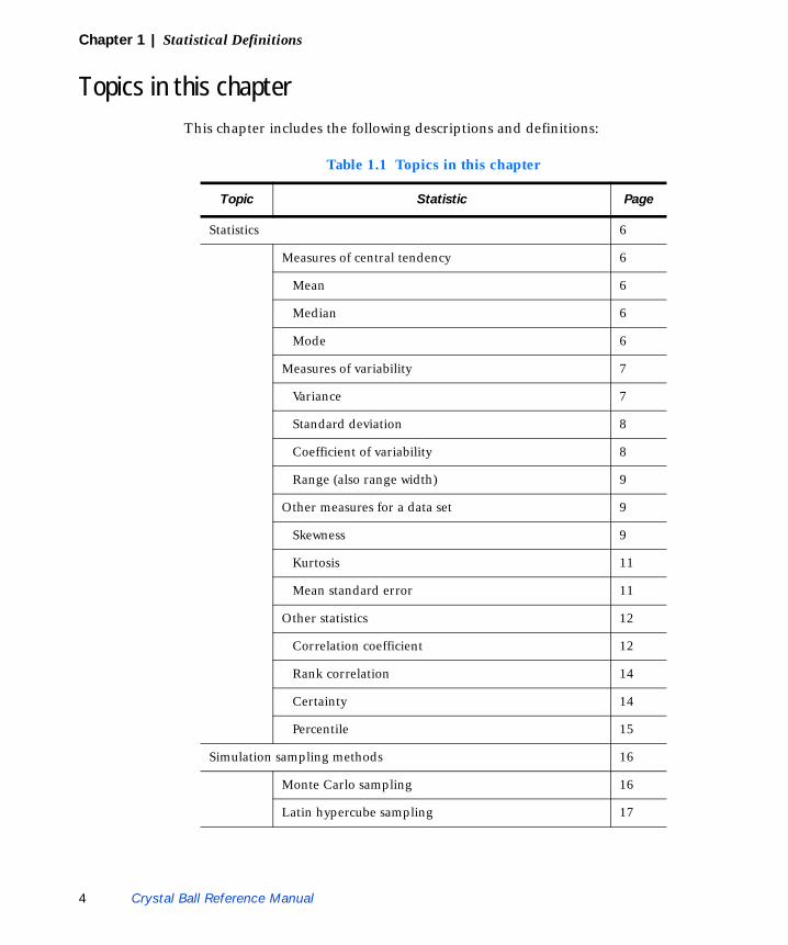
Topics in this chapterThis chapter includes the following descriptions and definitions:

Table 1.1 Topics in this chapter

Topic Statistic Page

Statistics 6

Measures of central tendency 6

Mean 6

Median 6

Mode 6

Measures of variability 7

Variance 7

Standard deviation 8

Coefficient of variability 8

Range (also range width) 9

Other measures for a data set 9

Skewness 9

Kurtosis 11

Mean standard error 11

Other statistics 12

Correlation coefficient 12

Rank correlation 14

Certainty 14

Percentile 15

Simulation sampling methods 16

Monte Carlo sampling 16

Latin hypercube sampling 17


Topics in this chapter1

Confidence intervals 18

Mean confidence interval 19

Standard deviation confidence interval 19

Percentiles confidence interval 19

Process capability metrics 20

Cp 20

Pp 20

Cpk-lower 21

Ppk-lower 21

Cpk-upper 21

Ppk-upper 21

Cpk 22

Ppk 22

Cpm 22

Ppm 23

Z-LSL 23

Z-USL 23

Zst 23

Zst-total 24

Zlt 24

Zlt-total 25

p(N/C)-below 25

p(N/C)-above 25

p(N/C)-total 26

PPM-below 26

PPM-above 26

Table 1.1 Topics in this chapter (Continued)




Statistics

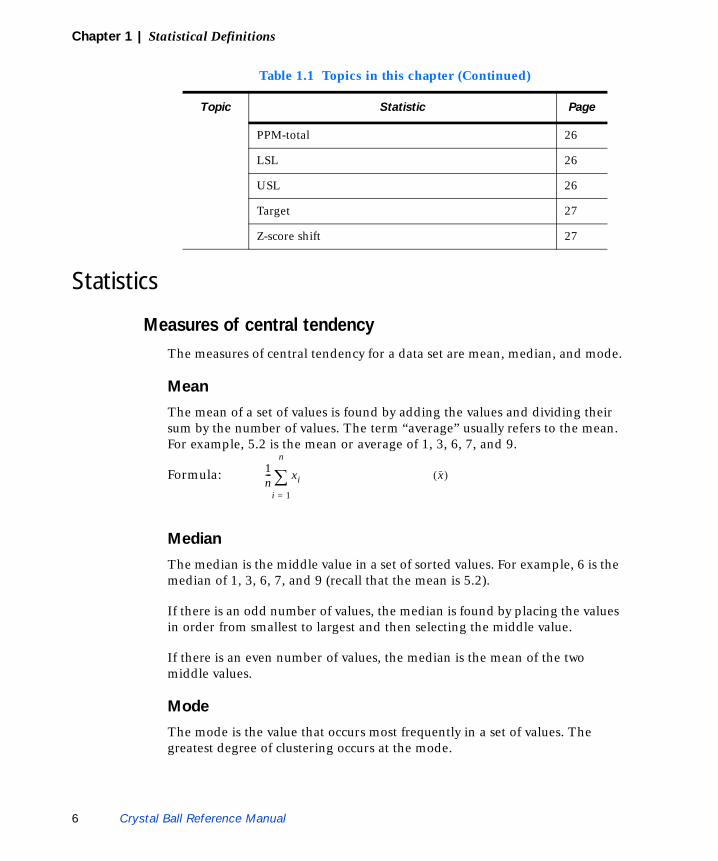
Measures of central tendencyThe measures of central tendency for a data set are mean, median, and mode.

Mean

The mean of a set of values is found by adding the values and dividing their sum by the number of values. The term “average” usually refers to the mean. For example, 5.2 is the mean or average of 1, 3, 6, 7, and 9.

Formula:

Median

The median is the middle value in a set of sorted values. For example, 6 is the median of 1, 3, 6, 7, and 9 (recall that the mean is 5.2).

If there is an odd number of values, the median is found by placing the values in order from smallest to largest and then selecting the middle value.

If there is an even number of values, the median is the mean of the two middle values.

Mode

The mode is the value that occurs most frequently in a set of values. The greatest degree of clustering occurs at the mode.

PPM-total 26

LSL 26

USL 26

Target 27

Z-score shift 27

Table 1.1 Topics in this chapter (Continued)


1n--- xi

i 1=

n

∑ x( )


Statistics1
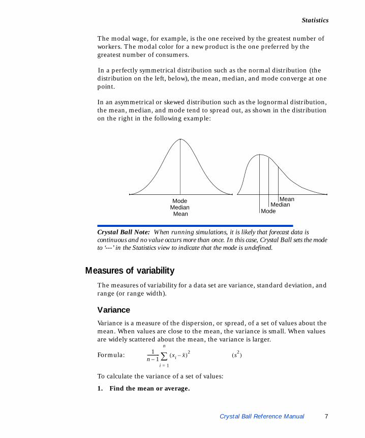
The modal wage, for example, is the one received by the greatest number of workers. The modal color for a new product is the one preferred by the greatest number of consumers.
In a perfectly symmetrical distribution such as the normal distribution (the distribution on the left, below), the mean, median, and mode converge at one point.

In an asymmetrical or skewed distribution such as the lognormal distribution, the mean, median, and mode tend to spread out, as shown in the distribution on the right in the following example:

Crystal Ball Note: When running simulations, it is likely that forecast data is continuous and no value occurs more than once. In this case, Crystal Ball sets the mode to ‘---’ in the Statistics view to indicate that the mode is undefined.

Measures of variabilityThe measures of variability for a data set are variance, standard deviation, and range (or range width).

Variance

Variance is a measure of the dispersion, or spread, of a set of values about the mean. When values are close to the mean, the variance is small. When values are widely scattered about the mean, the variance is larger.

Formula:

To calculate the variance of a set of values:

1. Find the mean or average.

ModeMedian

MeanMode Median Mean

1n 1–------------ xi x–( )2

i 1=

n

∑ s2( )



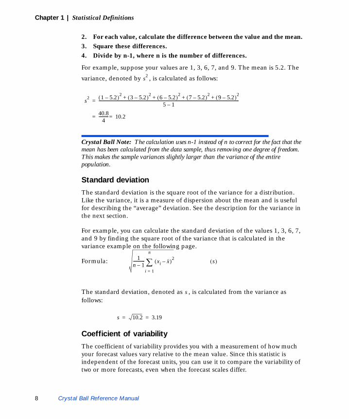
2. For each value, calculate the difference between the value and the mean.3. Square these differences.4. Divide by n-1, where n is the number of differences.

For example, suppose your values are 1, 3, 6, 7, and 9. The mean is 5.2. The

variance, denoted by , is calculated as follows:

Crystal Ball Note: The calculation uses n-1 instead of n to correct for the fact that the mean has been calculated from the data sample, thus removing one degree of freedom. This makes the sample variances slightly larger than the variance of the entire population.

Standard deviation

The standard deviation is the square root of the variance for a distribution. Like the variance, it is a measure of dispersion about the mean and is useful for describing the “average” deviation. See the description for the variance in the next section.

For example, you can calculate the standard deviation of the values 1, 3, 6, 7, and 9 by finding the square root of the variance that is calculated in the variance example on the following page.

Formula:

The standard deviation, denoted as , is calculated from the variance as follows:

Coefficient of variability

The coefficient of variability provides you with a measurement of how much your forecast values vary relative to the mean value. Since this statistic is independent of the forecast units, you can use it to compare the variability of two or more forecasts, even when the forecast scales differ.

s2

s2 1 5.2–( )2 3 5.2–( )2 6 5.2–( )2 7 5.2–( )2 9 5.2–( )2+ + + +5 1–

-------------------------------------------------------------------------------------------------------------------------------------------------=

40.84

---------- 10.2==

1n 1–------------ xi x–( )2

i 1=

n

∑ s( )

s

s 10.2 3.19= =


Statistics1
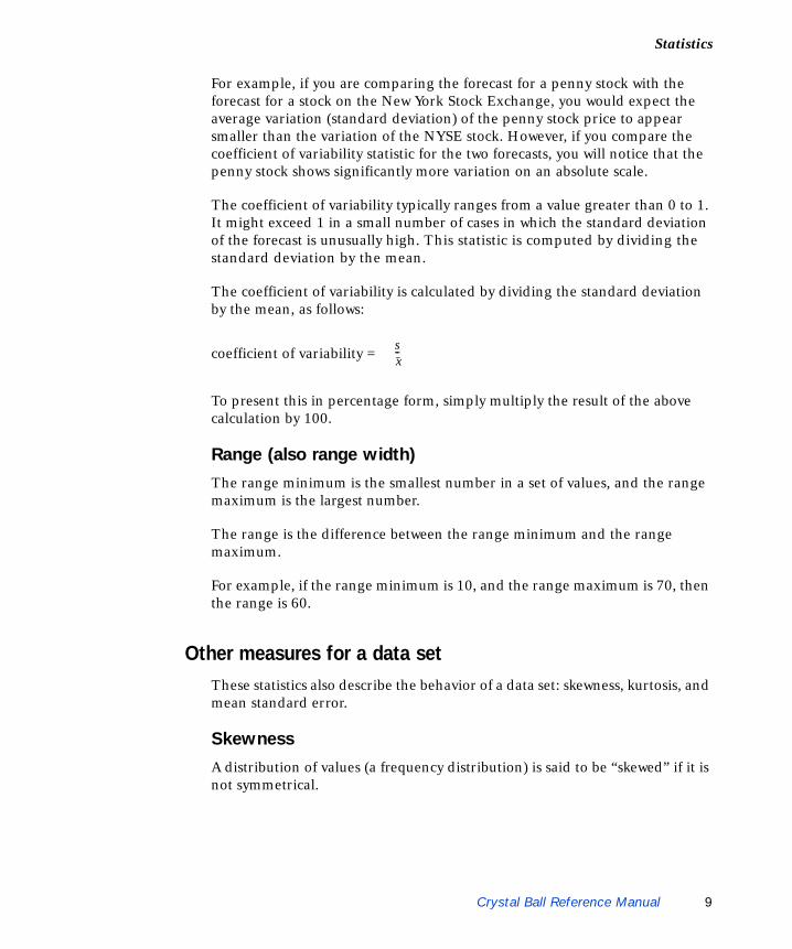
For example, if you are comparing the forecast for a penny stock with the forecast for a stock on the New York Stock Exchange, you would expect the average variation (standard deviation) of the penny stock price to appear smaller than the variation of the NYSE stock. However, if you compare the coefficient of variability statistic for the two forecasts, you will notice that the penny stock shows significantly more variation on an absolute scale.
The coefficient of variability typically ranges from a value greater than 0 to 1. It might exceed 1 in a small number of cases in which the standard deviation of the forecast is unusually high. This statistic is computed by dividing the standard deviation by the mean.

The coefficient of variability is calculated by dividing the standard deviation by the mean, as follows:

coefficient of variability =

To present this in percentage form, simply multiply the result of the above calculation by 100.

Range (also range width)

The range minimum is the smallest number in a set of values, and the range maximum is the largest number.

The range is the difference between the range minimum and the range maximum.

For example, if the range minimum is 10, and the range maximum is 70, then the range is 60.

Other measures for a data setThese statistics also describe the behavior of a data set: skewness, kurtosis, and mean standard error.

Skewness

A distribution of values (a frequency distribution) is said to be “skewed” if it is not symmetrical.

sx--



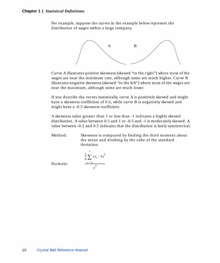
For example, suppose the curves in the example below represent the distribution of wages within a large company.

Curve A illustrates positive skewness (skewed “to the right”) where most of the wages are near the minimum rate, although some are much higher. Curve B illustrates negative skewness (skewed “to the left”) where most of the wages are near the maximum, although some are much lower.

If you describe the curves statistically, curve A is positively skewed and might have a skewness coefficient of 0.5, while curve B is negatively skewed and might have a -0.5 skewness coefficient.

A skewness value greater than 1 or less than -1 indicates a highly skewed distribution. A value between 0.5 and 1 or -0.5 and -1 is moderately skewed. A value between -0.5 and 0.5 indicates that the distribution is fairly symmetrical.

Method: Skewness is computed by finding the third moment about the mean and dividing by the cube of the standard deviation.

Formula:

A BA B

1n--- xi x–( )3

i 1=

n

∑

s3---------------------------------


Statistics1
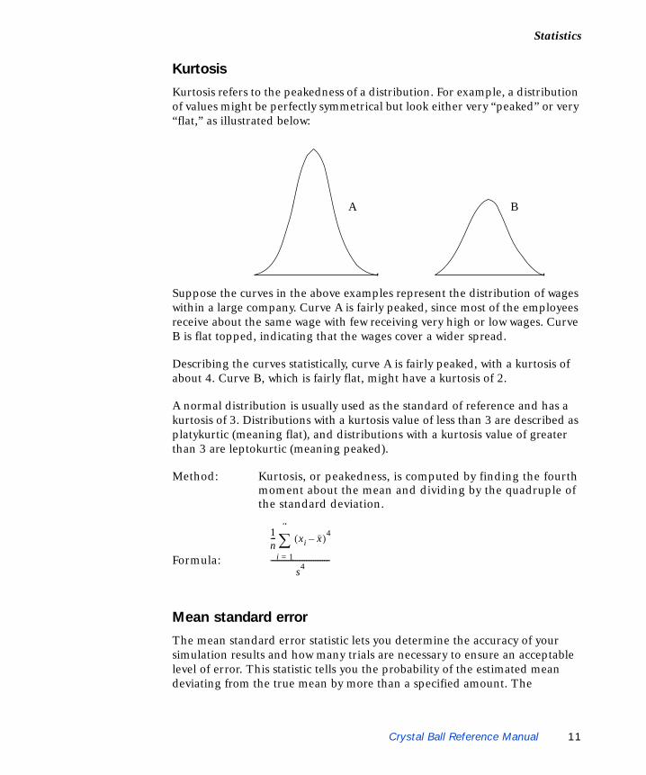
Kurtosis
Kurtosis refers to the peakedness of a distribution. For example, a distribution of values might be perfectly symmetrical but look either very “peaked” or very “flat,” as illustrated below:

Suppose the curves in the above examples represent the distribution of wages within a large company. Curve A is fairly peaked, since most of the employees receive about the same wage with few receiving very high or low wages. Curve B is flat topped, indicating that the wages cover a wider spread.

Describing the curves statistically, curve A is fairly peaked, with a kurtosis of about 4. Curve B, which is fairly flat, might have a kurtosis of 2.

A normal distribution is usually used as the standard of reference and has a kurtosis of 3. Distributions with a kurtosis value of less than 3 are described as platykurtic (meaning flat), and distributions with a kurtosis value of greater than 3 are leptokurtic (meaning peaked).

Method: Kurtosis, or peakedness, is computed by finding the fourth moment about the mean and dividing by the quadruple of the standard deviation.

Formula:

Mean standard error

The mean standard error statistic lets you determine the accuracy of your simulation results and how many trials are necessary to ensure an acceptable level of error. This statistic tells you the probability of the estimated mean deviating from the true mean by more than a specified amount. The

A BA B

1n--- xi x–( )4

i 1=

n

∑

s4---------------------------------



probability that the true mean of the forecast is the estimated mean (plus or minus the mean standard error) is approximately 68%.

Statistical Note: The mean standard error statistic only provides information on the accuracy of the mean and can be used as a general guide to the accuracy of the simulation. The standard error for other statistics, such as mode and median, will probably differ from the mean standard error.

Formula:

where: = Standard Deviation n = Number of Trials

The error estimate might be inverted to show the number of trials needed to yield a desired error .

Other statisticsThese statistics describe relationships between data sets (correlation coefficient, rank correlation) or other data measurements (certainty, percentile, confidence intervals).

Correlation coefficient

Crystal Ball Note: Crystal Ball uses rank correlation to determine the correlation coefficient of variables. For more information on rank correlation, see “Rank correlation” on page 14.

When the values of two variables depend upon one another in whole or in part, the variables are considered correlated. For example, an “energy cost” variable is likely to show a positive correlation with an “inflation” variable. When the “inflation” variable is high, the “energy cost” variable is also high; when the “inflation” variable is low, the “energy cost” variable is low.

In contrast, “product price” and “unit sale” variables might show a negative correlation. For example, when prices are low, sales are expected to be high; when prices are high, sales are expected to be low.

By correlating pairs of variables that have such a positive or negative relationship, you can increase the accuracy of your simulation forecast results.

sn

-------

s

ε( )

n s2

ε2-----=


Statistics1
The correlation coefficient is a number that describes the relationship between two dependent variables. Coefficient values range between -1 and 0 for a negative correlation and 0 and +1 for a positive correlation. The closer the absolute value of the correlation coefficient is to either +1 or -1, the more strongly the variables are related.
When an increase in one variable is associated with an increase in another variable, the correlation is called positive (or direct) and indicated by a coefficient between 0 and 1. When an increase in one variable is associated with a decrease in another variable, the correlation is called negative (or inverse) and indicated by a coefficient between 0 and -1. A value of 0 indicates that the variables are unrelated to one another. The example below shows three correlation coefficients.

For example, assume that total hotel food sales might be correlated with hotel room rates. Total food sales are likely to be higher, for example, at hotels with higher room rates. If food sales and room rates correspond closely for various hotels, the correlation coefficient is close to 1. However, the correlation might not be perfect (correlation coefficient < 1). Some people might eat meals outside the hotel while others might skip some meals altogether.

When you select a correlation coefficient to describe the relationship between a pair of variables in your simulation, you need to consider how closely they are related to one another. You should never need to use an actual correlation coefficient of 1 or -1. Generally, you should represent these types of relationships as formulas on your spreadsheet.

Formula:

Negative Correlation

Zero Correlation Positive Correlation

n xiyi

i 1=

n

∑ xi yi

i 1=

n

∑i 1=

n

∑–

n xi2 xi

i 1=

n

∑⎝ ⎠⎜ ⎟⎜ ⎟⎛ ⎞ 2

–i 1=

n

∑ n yi2 yi

i 1=

n

∑⎝ ⎠⎜ ⎟⎜ ⎟⎛ ⎞ 2

–i 1=

n

∑⋅

-------------------------------------------------------------------------------------------------------------



Crystal Ball Note: Crystal Ball uses rank correlation to correlate assumption values. This means that assumption values are replaced by their rankings from lowest to highest value by the integers 1 to n, prior to computing the correlation coefficient. This method allows distribution types to be ignored when correlating assumptions.

Rank correlation

A correlation coefficient measures the strength of the linear relationship between two variables. However, if the two variables do not have the same probability distributions, they are unlikely to be related linearly. Under those circumstances, the correlation coefficient calculated on their raw values has little meaning.

If you calculate the correlation coefficient using rank values instead of actual values, the correlation coefficient is meaningful even for variables with different distributions.

You determine rank values by arranging the actual values in ascending order and replacing the values with their rankings. For example, the lowest actual value will have a rank of 1, the next lowest actual value will have a rank of 2, etc.

Crystal Ball uses rank correlation to correlate assumptions. The slight loss of information that occurs using rank correlation is offset by a couple of advantages:

• First, the correlated assumptions need not have similar distribution types. In effect, the correlation function in Crystal Ball is distribution-independent. The rank correlation method even works when a distribution has been truncated at one or both ends of its range.

• Second, the values generated for each assumption are not changed, they are merely rearranged to produce the desired correlation. In this way, the original distributions of the assumptions are preserved.

Certainty

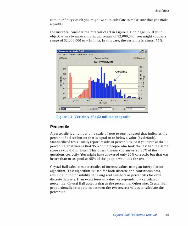
The forecast chart shows you not only the range of different results for each forecast, but also the probability, or certainty, of achieving results within a range. Certainty is the percent chance that a particular forecast value will fall within a specified range.

By default, the certainty range is from negative infinity to positive infinity. The certainty for this range is always 100%. However, you might want to estimate the chance of a forecast result falling in a specific range, say from


Statistics1
zero to infinity (which you might want to calculate to make sure that you make a profit).
For instance, consider the forecast chart in Figure 1.1 on page 15. If your objective was to make a minimum return of $2,000,000, you might choose a range of $2,000,000 to +Infinity. In this case, the certainty is almost 75%.

Figure 1.1 Certainty of a $2 million net profit

Percentile

A percentile is a number on a scale of zero to one hundred that indicates the percent of a distribution that is equal to or below a value (by default). Standardized tests usually report results in percentiles. So if you were at the 95 percentile, that means that 95% of the people who took the test had the same score as you did or lower. This doesn’t mean you answered 95% of the questions correctly. You might have answered only 20% correctly, but that was better than or as good as 95% of the people who took the test.

Crystal Ball calculates percentiles of forecast values using an interpolation algorithm. This algorithm is used for both discrete and continuous data, resulting in the possibility of having real numbers as percentiles for even discrete datasets. If an exact forecast value corresponds to a calculated percentile, Crystal Ball accepts that as the percentile. Otherwise, Crystal Ball proportionally interpolates between the two nearest values to calculate the percentile.

Certainty



Crystal Ball Note: When calculating medians, Crystal Ball does not use the proportional interpolation algorithm. It uses the classical definition of median, described on page 6.

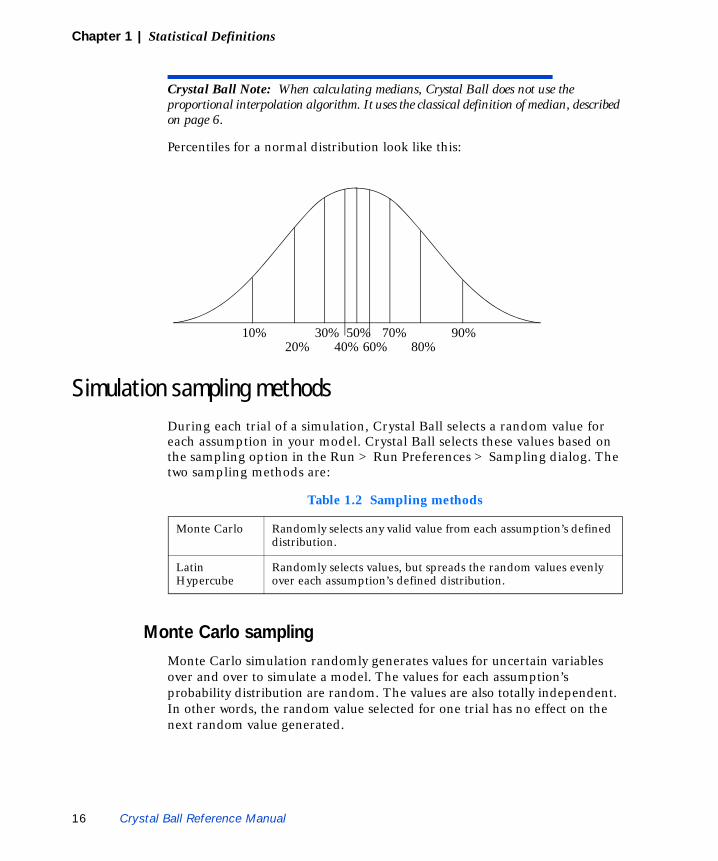
Percentiles for a normal distribution look like this:

Simulation sampling methodsDuring each trial of a simulation, Crystal Ball selects a random value for each assumption in your model. Crystal Ball selects these values based on the sampling option in the Run > Run Preferences > Sampling dialog. The two sampling methods are:

Monte Carlo samplingMonte Carlo simulation randomly generates values for uncertain variables over and over to simulate a model. The values for each assumption’s probability distribution are random. The values are also totally independent. In other words, the random value selected for one trial has no effect on the next random value generated.

10% 30% 50% 70% 90%20% 40% 60% 80%

Table 1.2 Sampling methods

Monte Carlo Randomly selects any valid value from each assumption’s defined distribution.

Latin Hypercube

Randomly selects values, but spreads the random values evenly over each assumption’s defined distribution.


Simulation sampling methods1
Monte Carlo simulation was named for Monte Carlo, Monaco, where the primary attractions are casinos containing games of chance. Games of chance such as roulette wheels, dice, and slot machines exhibit random behavior.
The random behavior in games of chance is similar to how Monte Carlo simulation selects variable values at random to simulate a model. When you roll a die, you know that either a 1, 2, 3, 4, 5, or 6 will come up, but you don’t know which for any particular trial. It is the same with the variables that have a known range of values but an uncertain value for any particular time or event (e.g., interest rates, staffing needs, stock prices, inventory, phone calls per minute).

Using Monte Carlo sampling to approximate the true shape of the distribution requires a larger number of trials than Latin hypercube.

Use Monte Carlo sampling when you want to simulate “real world” what-if scenarios for your spreadsheet model.

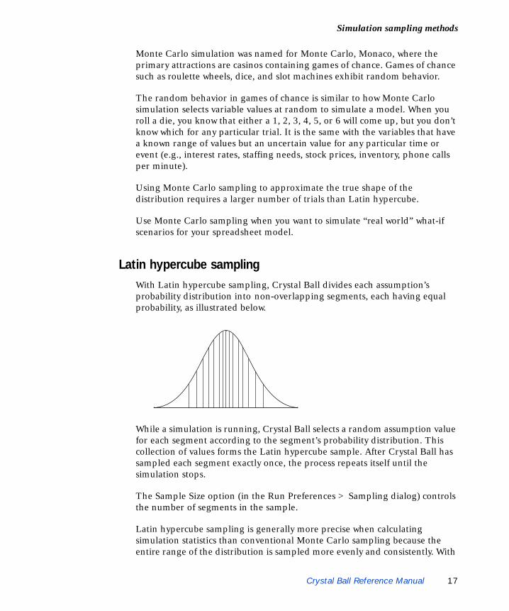
Latin hypercube samplingWith Latin hypercube sampling, Crystal Ball divides each assumption’s probability distribution into non-overlapping segments, each having equal probability, as illustrated below.

While a simulation is running, Crystal Ball selects a random assumption value for each segment according to the segment’s probability distribution. This collection of values forms the Latin hypercube sample. After Crystal Ball has sampled each segment exactly once, the process repeats itself until the simulation stops.

The Sample Size option (in the Run Preferences > Sampling dialog) controls the number of segments in the sample.

Latin hypercube sampling is generally more precise when calculating simulation statistics than conventional Monte Carlo sampling because the entire range of the distribution is sampled more evenly and consistently. With



Latin hypercube sampling, you don’t need as many trials to achieve the same level of statistical accuracy as with Monte Carlo sampling. The added expense of this method is the extra memory required to track which segments have been sampled while the simulation runs. (Compared to most simulation results, this extra overhead is minor.)

Use Latin hypercube sampling when you are concerned primarily with the accuracy of the simulation statistics.

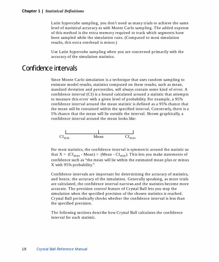
Confidence intervalsSince Monte Carlo simulation is a technique that uses random sampling to estimate model results, statistics computed on these results, such as mean, standard deviation and percentiles, will always contain some kind of error. A confidence interval (CI) is a bound calculated around a statistic that attempts to measure this error with a given level of probability. For example, a 95% confidence interval around the mean statistic is defined as a 95% chance that the mean will be contained within the specified interval. Conversely, there is a 5% chance that the mean will lie outside the interval. Shown graphically, a confidence interval around the mean looks like:

For most statistics, the confidence interval is symmetric around the statistic so that X = (CImax - Mean) = (Mean - CImin). This lets you make statements of confidence such as “the mean will lie within the estimated mean plus or minus X with 95% probability.”

Confidence intervals are important for determining the accuracy of statistics, and hence, the accuracy of the simulation. Generally speaking, as more trials are calculated, the confidence interval narrows and the statistics become more accurate. The precision control feature of Crystal Ball lets you stop the simulation when the specified precision of the chosen statistics is reached. Crystal Ball periodically checks whether the confidence interval is less than the specified precision.

The following sections describe how Crystal Ball calculates the confidence interval for each statistic.

CImin Mean CImax


Random number generation1
Mean confidence interval
Formula:

where:

s is the standard deviation of the forecast n is the number of trials z is the z-value based on the specified confidence level (in the Run Preferences > Trials tab).

Standard deviation confidence interval

Formula:

where:

s is the standard deviation k is the kurtosis n is the number of trials z is the z-value based on the specified confidence level (in Run Preferences > Trials tab).

Percentiles confidence intervalTo calculate the confidence interval for the percentiles, instead of a mathematical formula, Crystal Ball uses an analytical bootstrapping method.

Random number generationCrystal Ball uses the random number generator given below as the basis for all of the non-uniform generators. For no starting seed value, Crystal Ball takes the value of the number of milliseconds elapsed since Windows started.

Method: Multiplicative Congruential Generator This routine uses the iteration formula:

r

z sn

-------⋅

z s k 1–4 n 1–( )⋅------------------------⋅ ⋅

62089911 r•( ) mod 231 1 )–(



Comment: The generator has a period of length , or 2,147,483,646. This means that the cycle of random numbers repeats after several billion trials. This formula is discussed in detail in the Simulation Modeling & Analysis and Art of Computer Programming, Vol. II, references in the Bibliography.

Process capability metricsThe Crystal Ball process capability metrics are provided to support quality improvement methodologies such as Six Sigma, DFSS (Design for Six Sigma), and Lean Principles. They appear in forecast charts when a forecast definition includes a lower specification limit (LSL), upper specification limit (USL), or both. Optionally, a target value can also be included in the definition.

The following sections describe capability metrics calculated by Crystal Ball. In general, capability indices beginning with C (such as Cpk) are for short-term data while their long-term equivalents begin with P (such as Ppk).

CpShort-term capability index indicating what quality level the forecast output is potentially capable of producing. It is defined as the ratio of the specification width to the forecast width. If a Cp is equal to or greater than 1, then a short-term 3-sigma quality level is possible.

PpLong-term capability index indicating what quality level the forecast output is potentially capable of producing. It is defined as the ratio of the specification width to the forecast width. If a Pp is equal to or greater than 1, then a short-term 3-sigma quality level is possible.

231 2–

CpUSL LSL–

6σ---------------------------=

PpUSL LSL–

6σ---------------------------=


Process capability metrics1
Cpk-lower
One-sided short-term capability index; for normally distributed forecasts, the ratio of the difference between the forecast mean and lower specification limit over three times the forecast short-term standard deviation; often used to calculate process capability indices with only a lower specification limit.

Ppk-lowerOne-sided long-term capability index; for normally distributed forecasts, the ratio of the difference between the forecast mean and lower specification limit over three times the forecast long-term standard deviation; often used to calculate process capability indices with only a lower specification limit.

Cpk-upperOne-sided short-term capability index; for normally distributed forecasts, the ratio of the difference between the forecast mean and upper specification limit over three times the forecast short-term standard deviation; often used to calculate process capability indices with only an upper specification limit.

Ppk-upperOne-sided long-term capability index; for normally distributed forecasts, the ratio of the difference between the forecast mean and upper specification limit over three times the forecast long-term standard deviation; often used to calculate process capability indices with only an upper specification limit.

Cpk LOWER–μ LSL–

3σ-------------------=

Ppk LOWER–μ LSL–

3σ-------------------=

Cpk UPPER–USL μ–

3σ--------------------=

Ppk UPPER–USL μ–

3σ--------------------=



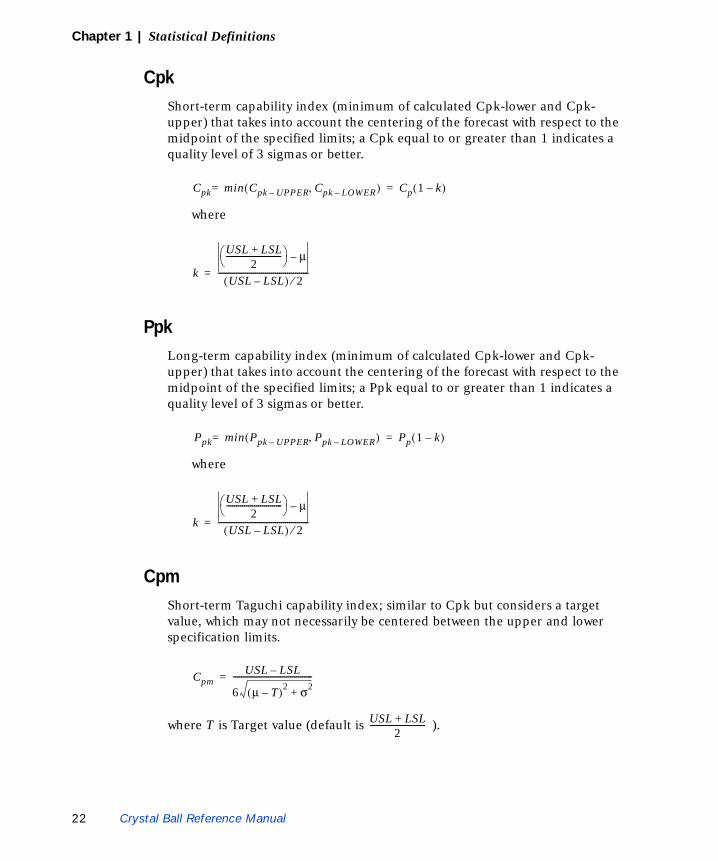
CpkShort-term capability index (minimum of calculated Cpk-lower and Cpk-upper) that takes into account the centering of the forecast with respect to the midpoint of the specified limits; a Cpk equal to or greater than 1 indicates a quality level of 3 sigmas or better.

where

PpkLong-term capability index (minimum of calculated Cpk-lower and Cpk-upper) that takes into account the centering of the forecast with respect to the midpoint of the specified limits; a Ppk equal to or greater than 1 indicates a quality level of 3 sigmas or better.

where

CpmShort-term Taguchi capability index; similar to Cpk but considers a target value, which may not necessarily be centered between the upper and lower specification limits.

where T is Target value (default is ).

Cpk min Cpk UPPER– Cpk LOWER–,( )= Cp 1 k–( )=

k

USL LSL+2

----------------------------⎝ ⎠⎛ ⎞ μ–

USL LSL–( ) 2⁄----------------------------------------------=

Ppk min Ppk UPPER– Ppk LOWER–,( )= Pp 1 k–( )=

k

USL LSL+2

----------------------------⎝ ⎠⎛ ⎞ μ–

USL LSL–( ) 2⁄----------------------------------------------=

CpmUSL LSL–

6 μ T–( )2 σ2+----------------------------------------=

USL LSL+2

----------------------------



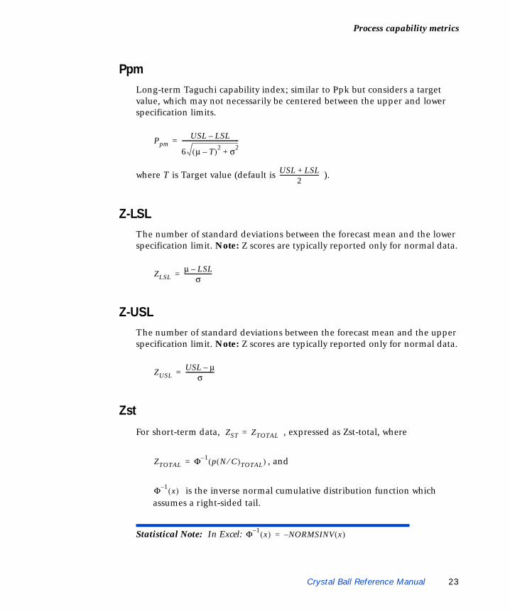
PpmLong-term Taguchi capability index; similar to Ppk but considers a target value, which may not necessarily be centered between the upper and lower specification limits.

where T is Target value (default is ).

Z-LSLThe number of standard deviations between the forecast mean and the lower specification limit. Note: Z scores are typically reported only for normal data.

Z-USLThe number of standard deviations between the forecast mean and the upper specification limit. Note: Z scores are typically reported only for normal data.

Zst

For short-term data, , expressed as Zst-total, where

, and

is the inverse normal cumulative distribution function which assumes a right-sided tail.

Statistical Note: In Excel:

PpmUSL LSL–

6 μ T–( )2 σ2+----------------------------------------=

USL LSL+2

----------------------------

ZLSLμ LSL–

σ-------------------=

ZUSLUSL μ–

σ--------------------=

ZST ZTOTAL=

ZTOTAL Φ 1– p N C⁄( )TOTAL( )=

Φ 1– x( )

Φ 1– x( ) NORMSINV x( )–=



When displaying short-term metrics, appears as Zst-total. This metric is equal to Z-LSL if there is only a lower specification limit or Z-USL if there is only an upper specification limit.

For long-term data, . When displaying long-term

metrics, appears in the capability metrics table as Zst.

Note: Z scores are typically reported only for normal data. The maximum value for Z scores calculated by Crystal Ball from forecast data is 8.00.

Zst-totalFor short-term metrics when both specification limits are defined, the number of standard deviations between the short-term forecast mean and the lower boundary of combining all defects onto the upper tail of the normal curve. Also equal to Zlt-total plus the Z-score shift value if long-term metrics are calculated.

When short-term metrics are calculated, Zst-total is equivalent to , described in the previous section.

Note: Z scores are typically reported only for normal data.

Zlt

For long-term data, , expressed as Zlt-total, where

, and

is the inverse normal cumulative distribution function which assumes a right-sided tail.


When displaying long-term metrics, appears as Zlt-total. This metric is equal to Z-LSL if there is only a lower specification limit or Z-USL if there is only an upper specification limit.

ZST

ZST ZLT ZScoreShift+=

ZST

ZST

ZLT ZTOTAL=

ZTOTAL Φ 1– p N C⁄( )TOTAL( )=

Φ 1– x( )

Φ 1– x( ) NORMSINV x( )–=

ZLT


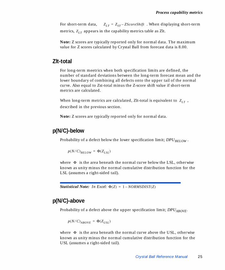
For short-term data, . When displaying short-term
metrics, appears in the capability metrics table as Zlt.

Note: Z scores are typically reported only for normal data. The maximum value for Z scores calculated by Crystal Ball from forecast data is 8.00.

Zlt-totalFor long-term meetrics when both specification limits are defined, the number of standard deviations between the long-term forecast mean and the lower boundary of combining all defects onto the upper tail of the normal curve. Also equal to Zst-total minus the Z-score shift value if short-term metrics are calculated.

When long-term metrics are calculated, Zlt-total is equivalent to , described in the previous section.

Note: Z scores are typically reported only for normal data.

p(N/C)-belowProbability of a defect below the lower specification limit; DPUBELOW .

where is the area beneath the normal curve below the LSL, otherwise known as unity minus the normal cumulative distribution function for the LSL (assumes a right-sided tail).


p(N/C)-aboveProbability of a defect above the upper specification limit; DPUABOVE.

where is the area beneath the normal curve above the USL, otherwise known as unity minus the normal cumulative distribution function for the USL (assumes a right-sided tail).

ZLT ZST ZScoreShift–=

ZLT

ZLT

p N C⁄( )BELOW Φ ZLSL( )=

Φ

Φ Z( ) 1 NORMSDIST Z( )–=

p N C⁄( )ABOVE Φ ZUSL( )=

Φ




p(N/C)-totalProbability of a defect outside the lower and upper specification limits; DPUTOTAL.

PPM-belowDefects below the lower specification limit, per million units.

PPM-aboveDefects above the upper specification limit, per million units.

PPM-totalDefects outside both specification limits, per million units.

LSLLower specification limit; the lowest acceptable value of a forecast involved in process capability, or quality, analysis. User-defined by direct entry or reference when defining a forecast.

USLUpper specification limit; the highest acceptable value of a forecast involved in process capability, or quality, analysis. User-defined by direct entry or reference when defining a forecast.

Φ Z( ) 1 NORMSDIST Z( )–=

p N C⁄( )TOTAL p N C⁄( )ABOVE p N C⁄( )BELOW+=

PPMBELOW p N C⁄( )BELOW 106•=

PPMABOVE p N C⁄( )ABOVE 106•=

PPMTOTAL PPMABOVE PPMBELOW+=


Target
The ideal target value of a forecast involved in process capability analysis. User-defined by direct entry or reference when defining a forecast.

Z-score shiftAn optional shift value to use when calculating long-term capability metrics. The default, set in the Capability Options dialog, is 1.5.


Chapter 2Equations and Methods

In this chapterThis chapter provides formulas for the probability distributions.

Formulas for other statistical terms are included in Chapter 1.


Chapter 2 | Equations and Methods

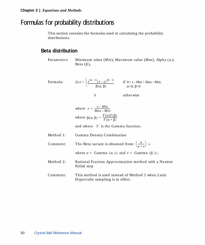
Formulas for probability distributionsThis section contains the formulas used in calculating the probability distributions.

Beta distribution

Parameters: Minimum value (Min), Maximum value (Max), Alpha ( ), Beta ( ),

Formula: if

otherwise

where

where

and where is the Gamma function.

Method 1: Gamma Density Combination

Comment: The Beta variate is obtained from:

where u = Gamma and v = Gamma .

Method 2: Rational Fraction Approximation method with a Newton Polish step

Comment: This method is used instead of Method 1 when Latin Hypercube sampling is in effect.

αβ

f x( ) z α 1–( ) 1 z–( ) β 1–( )

β α β,( )----------------------------------------------

⎩⎨⎧

= 0< x - Min < Max - Min;α>0; β>0

0

z x Min–Max Min–---------------------------=

β α β,( )Γ α( )Γ β( )Γ α β+( )-------------------------=

Γ

uu v+------------⎝ ⎠⎛ ⎞ s⋅

α 1,( ) β 1,( )


Formulas for probability distributions1

BetaPERT distribution

Parameters: Minimum value (Min), Most likely value (Likeliest), Maximum value (Max)

Formula: for

Where

,

And

is the beta integral.

Binomial distribution

Parameters: Probability of success (p), Number of total trials (n)

Formula:

for i = 0,1,2,...n; p > 0; 0 < n < 1,000

where

and x = number of successful trials

Method: Direct Simulation

Comment: Computation time increases linearly with number of trials.

f x( ) x Min )–( α 1– Max x–( )β 1–

B α β,( ) Max Min–( )α β 1–+----------------------------------------------------------------------= Min x Max≤ ≤

α 6 μ Min–Max Min–---------------------------⎝ ⎠⎛ ⎞=

β 6 Max μ–Max Min–---------------------------⎝ ⎠⎛ ⎞=

μ Min 4 Likely Max+×+6

------------------------------------------------------------=

B α β,( )

P x{ i } ni⎝ ⎠

⎛ ⎞ pi 1 p ) n i–( )–(==

ni⎝ ⎠

⎛ ⎞ n!i! n i )!–(----------------------=



Discrete uniform distribution

Parameters: Minimum value (Min), Maximum value (Max)

Formula:

Comment: This is the discrete equivalent of the uniform distribution, described on page 38.

Exponential distribution

Parameters: Success rate

Formula: if x 0 and if x < 0

Method: Inverse Transformation

Gamma distributionThis distribution includes the Erlang and Chi-Square distributions as special cases.

Parameters: Location (L), Scale (s), Shape

Formula:

where is the gamma function

Note: some textbook Gamma formulas use:

Method 1: When , Vaduva’s rejection from a Weibull density.

f x( )1

Max Min– 1+( )------------------------------------------

0 otherwise⎩⎪⎨⎪⎧

=if Min x Max< <

λ( )

f x( ) λe λ– x

0⎩⎨⎧

= ≥ λ 0>

β( )

f x( )

x L–s

------------⎝ ⎠⎛ ⎞ β 1–

ex L–

s------------–

Γ β( )s------------------------------------------

0⎩ ⎭⎪ ⎪⎪ ⎪⎨ ⎬⎪ ⎪⎪ ⎪⎧ ⎫

= if x > L, 0 < β ∞ 0 s ∞< <,<

if x L≤

Γ

s 1λ---=

β 1<



When , Best’s rejection from a t density with 2 degrees of freedom.

When , inverse transformation.

Method 2: Rational Fraction Approximation method with a Newton Polish step

Comment: This method is used instead of Method 1 when Latin Hypercube sampling is in effect.

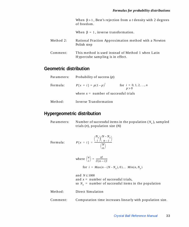
Geometric distribution

Parameters: Probability of success (p)

Formula: for

where x = number of successful trials


Hypergeometric distribution

Parameters: Number of successful items in the population ( ), sampled trials (n), population size (N)

Formula:

where

for

and and x = number of successful trials, so = number of successful items in the population

Method: Direct Simulation

Comment: Computation time increases linearly with population size.

β 1>

β 1=

P x{ i } p 1 p )i–(== i 0 1 2 … np 0>

, , , ,=

Nx

P x{ i }

Nxi⎝ ⎠

⎛ ⎞ N Nx–n i–⎝ ⎠

⎛ ⎞

Nn⎝ ⎠⎛ ⎞

----------------------------------= =

ni⎝ ⎠

⎛ ⎞ n!i! n i )!–(----------------------=

i Max n N Nx ) 0 ), …–(–(= Min n Nx ),(

N 1000≤

Nx



Logistic distribution

Parameters: Mean , Scale

Formula: for

where


Lognormal distribution

Parameters: Mean , Standard Deviation

Translation from arithmetic to log parameters: Log mean = =

Log standard deviation = =

where ln = natural logarithm

Formula: for

Method: Polar Marsaglia

Comment: A Normal variate in log space is generated and then exponentiated.

Additional formulas:

Geometric mean =

Geometric std. dev. =

Translation from log to arithmetic parameters:

Median = geometric mean

μ( ) s( )

f x( ) zs 1 z+( )2---------------------= ∞ x ∞

0 s ∞∞ μ ∞< <–

,< <–,< <–

z e

x μ–s

------------⎝ ⎠⎛ ⎞–

=

μ( ) σ( )

μlogμ

eσlog( )2

2----------------

---------------

⎝ ⎠⎜ ⎟⎜ ⎟⎜ ⎟⎛ ⎞

ln

σlog e2 σ

μ---ln⋅

1+⎝ ⎠⎜ ⎟⎛ ⎞

ln

f x( ) 1x 2π σlog

-------------------------- ex( )ln μlog–[ ]2 2σlog

2⁄–= x 0

μ 0σ 0>

>>

eμlog

eσlog



Mean =

Standard deviation=

Maximum extreme distributionThe maximum extreme distribution is the positively skewed form of the extreme value distribution.

Parameters: Likeliest (m), Scale (s)

Formula: for , , and

where

Method: Inverse Transformation.

Minimum extreme distributionThe minimum extreme distribution is the negatively skewed form of the extreme value distribution.

Parameters: Likeliest (m), Scale (s)

Formula: for , , and

where


median e

σlog2

2------------⎝ ⎠⎛ ⎞

⋅

median eσlog

2

eσlog

2

1–⎝ ⎠⎛ ⎞⋅⋅

f x( ) 1s--- z e z–⋅ ⋅= ∞– x ∞< <

∞ m ∞< <–s 0>

z e

x m–( )–s

---------------------⎝ ⎠⎛ ⎞

=

f x( ) 1s--- z e z–⋅ ⋅= ∞– x ∞< <

∞ m ∞< <–s 0>

z e

x m–s

-------------⎝ ⎠⎛ ⎞

=



Negative binomial distribution

Parameters: Probability of success (p), Shape ( )

Formula: for p > 0 and

where and x = number of successful trials

Method: Direct Simulation through summation of Geometric variates

Comment: Computation time increases linearly with Shape.

Normal distributionThis distribution is also known as the Gaussian distribution.

Parameters: Mean , Standard Deviation

Formula: for

Method 1: Polar Marsaglia

Comment: This method is somewhat slower than other methods, but its accuracy is essentially perfect.

Method 2: Rational Fraction Approximation

Comment: This method is used instead of the Polar Marsaglia method when Latin Hypercube sampling is in effect.

This method has a 7-8 digit accuracy over the central range of the distribution and a 5-6 digit accuracy in the tails.

β

P x{ i }x 1–β 1–⎝ ⎠⎛ ⎞ pβ 1 p–( )x β–

0⎩⎪⎨⎪⎧

==i β β 1

β 2 …,+,+,=

x 1–β 1–⎝ ⎠⎛ ⎞ x 1–( )!

β 1–( )! x β–( )!--------------------------------------=

μ( ) σ( )

f x( ) 12π σ

----------------e x μ )2 2σ2⁄–(–= ∞ x ∞∞ μ ∞

σ 0>< <–< <–



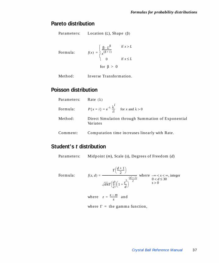
Pareto distribution

Parameters: Location (L), Shape

Formula:

for > 0


Poisson distribution

Parameters: Rate

Formula:

Method: Direct Simulation through Summation of Exponential Variates

Comment: Computation time increases linearly with Rate.

Student’s t distribution

Parameters: Midpoint (m), Scale (s), Degrees of Freedom (d)

Formula: where

where and

where = the gamma function,

β( )

f x( )β Lβ⋅x β 1+( )----------------

0⎩⎪⎨⎪⎧

=

if x L>

if x L≤

β

λ( )

P x i={ } e λ– λi

i!-----= for x and λ 0>

f z d,( )Γ d 1+

2------------⎝ ⎠⎛ ⎞

dπΓ d2---⎝ ⎠⎛ ⎞ 1 z2

d----+⎝ ⎠

⎛ ⎞

d 1+( )2

---------------------------------------------------------------------------= ∞ x ∞, integer

0 d 30s 0>

≤<< <–

z x m–s

-------------=

Γ



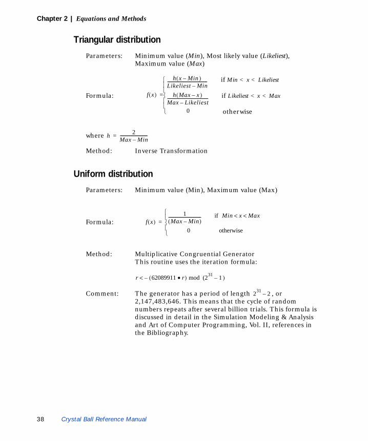
Triangular distribution

Parameters: Minimum value (Min), Most likely value (Likeliest), Maximum value (Max)

if Min < x < Likeliest

Formula: if Likeliest < x < Max

otherwise

where


Uniform distribution

Parameters: Minimum value (Min), Maximum value (Max)

Formula:

Method: Multiplicative Congruential Generator This routine uses the iteration formula:

Comment: The generator has a period of length , or 2,147,483,646. This means that the cycle of random numbers repeats after several billion trials. This formula is discussed in detail in the Simulation Modeling & Analysis and Art of Computer Programming, Vol. II, references in the Bibliography.

f x( )

h x Min )–(Likeliest Min–---------------------------------------

h Max x )–(Max Likeliest–----------------------------------------

0⎩⎪⎪⎨⎪⎪⎧

=

h 2Max Min–---------------------------=

f x( )1

Max Min–( )--------------------------------

0 otherwise⎩⎪⎨⎪⎧

=if Min x Max< <

r 62089911 r•( ) mod (231– 1 )–<

231 2–



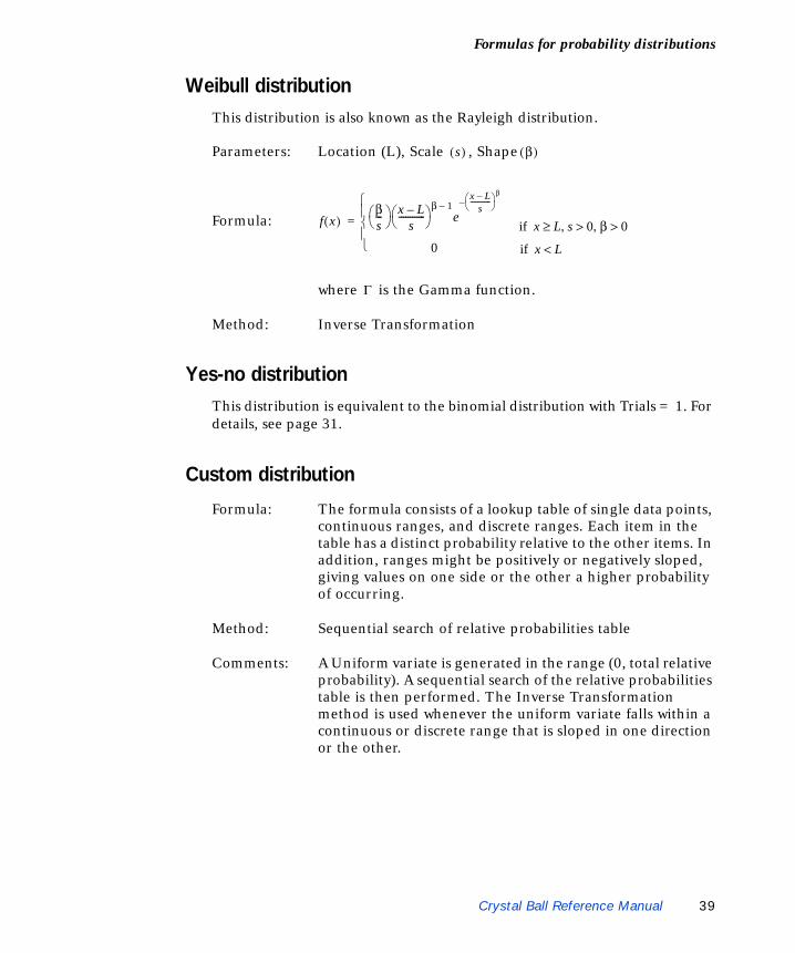
Weibull distributionThis distribution is also known as the Rayleigh distribution.

Parameters: Location (L), Scale , Shape

Formula:

where is the Gamma function.


Yes-no distributionThis distribution is equivalent to the binomial distribution with Trials = 1. For details, see page 31.

Custom distribution

Formula: The formula consists of a lookup table of single data points, continuous ranges, and discrete ranges. Each item in the table has a distinct probability relative to the other items. In addition, ranges might be positively or negatively sloped, giving values on one side or the other a higher probability of occurring.

Method: Sequential search of relative probabilities table

Comments: A Uniform variate is generated in the range (0, total relative probability). A sequential search of the relative probabilities table is then performed. The Inverse Transformation method is used whenever the uniform variate falls within a continuous or discrete range that is sloped in one direction or the other.

s( ) β( )

f x( )βs---⎝ ⎠⎛ ⎞ x L–

s------------⎝ ⎠⎛ ⎞ β 1–

e

x L–s

------------⎝ ⎠⎛ ⎞ β

–

0⎩⎪⎨⎪⎧

= if x L s 0 β 0>,>,≥

if x L<

Γ



Additional commentsAll of the non-uniform generators use the same uniform generator as the basis for their algorithms.

The Inverse Transformation method is based on the property that the cumulative distribution function for any probability distribution increases monotonically from zero to one. Thus, the inverse of this function can be computed using a random uniform variate in the range (0, 1) as input. The resulting values then have the desired distribution.

The Direct Simulation method actually performs a series of experiments on the selected distribution. For example, if a binomial variate is being generated with Prob = .5 and Trials = 20, then 20 uniform variates in the range (0, 1) are generated and compared with Prob. The number of uniform variates found to be less than Prob then becomes the value of the binomial variate.

Distribution fitting methodsDuring distribution fitting, Crystal Ball computes Maximum Likelihood Estimators (MLEs) to fit most of the probability distributions to a data set. In effect, this method chooses values for the parameters of the distributions that maximize the probability of producing the actual data set. Sometimes, however, the MLEs do not exist for some distributions (e.g., gamma, beta). In these cases, Crystal Ball resorts to other natural parameter estimation techniques.

When the MLEs do exist, they exhibit desirable properties:

• They are minimum-variance estimators of the parameters.

• As the data set grows, the biases in the MLEs tend to zero.

For several of the distributions (e.g. uniform, exponential), it is possible to remove the biases after computing the MLEs to yield minimum-variance unbiased estimators (MVUEs) of the distribution parameters. These MVUEs are the best possible estimators.


Chapter 3Default Names and Distribution Parameters

In this chapter• Naming defaults

• Distribution parameter defaults

This first section of this chapter describes the process Crystal Ball uses to name assumptions, decision variables, and forecasts. The second section shows the values it assigns to each of the distribution types.


Chapter 3 | Default Names and Distribution Parameters

Naming defaultsWhen defining an assumption, decision variable, or forecast, Crystal Ball uses the following sequence to generate a default name for the data cell:

1. Checks for a range name and if found, uses it as the cell name.

2. Checks the cell immediately to the left of the selected cell. If it is a text cell, Crystal Ball uses that text as the cell name.

3. Checks the cell immediately above the selected cell. If it is a text cell, Crystal Ball uses that text as the cell name.

4. If there is no applicable text or range name, Crystal Ball uses the cell coordinates for the name (for example, B3 or C7).


Distribution parameter defaults1

Distribution parameter defaultsThis section lists the initial values Crystal Ball provides for the primary parameters in the Define Assumption dialog:

• Beta• BetaPERT• Binomial• Custom• Discrete uniform• Exponential• Gamma• Geometric• Hypergeometric• Logistic• Lognormal• Maximum extreme value• Minimum extreme value• Negative binomial• Normal• Pareto• Poisson• Student’s t• Triangular• Uniform• Weibull• Yes-No

If an alternate parameter set is selected as the default mode, the primary parameters are still calculated as described below before conversion to the alternate parameters.

Statistical Note: Extreme values on the order of 1e±9 or ±1e16 may yield somewhat different results from those listed here.



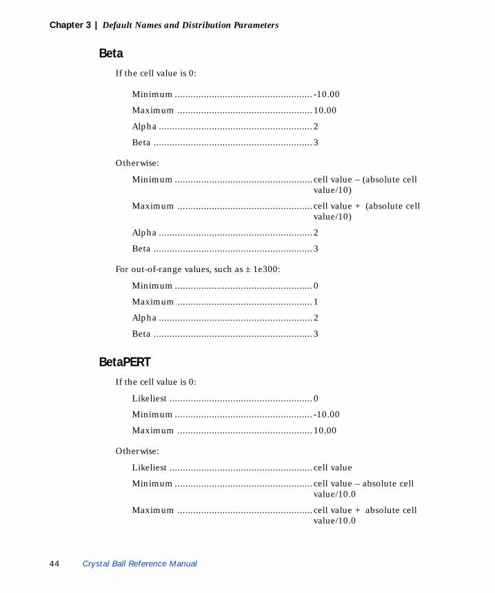
BetaIf the cell value is 0:

Minimum .................................................... -10.00

Maximum ................................................... 10.00

Alpha .......................................................... 2

Beta ............................................................ 3

Otherwise:

Minimum .................................................... cell value – (absolute cell value/10)

Maximum ................................................... cell value + (absolute cell value/10)

Alpha .......................................................... 2

Beta ............................................................ 3

For out-of-range values, such as ±1e300:

Minimum .................................................... 0

Maximum ................................................... 1

Alpha .......................................................... 2

Beta ............................................................ 3

BetaPERTIf the cell value is 0:

Likeliest ...................................................... 0

Minimum .................................................... -10.00

Maximum ................................................... 10.00

Otherwise:

Likeliest ...................................................... cell value

Minimum .................................................... cell value – absolute cell value/10.0

Maximum ................................................... cell value + absolute cell value/10.0



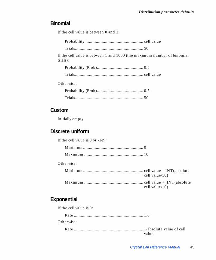
BinomialIf the cell value is between 0 and 1:

Probability ................................................. cell value

Trials........................................................... 50

If the cell value is between 1 and 1000 (the maximum number of binomial trials):

Probability (Prob)........................................ 0.5

Trials........................................................... cell value

Otherwise:

Probability (Prob)........................................ 0.5

Trials........................................................... 50

CustomInitially empty

Discrete uniformIf the cell value is 0 or -1e9:

Minimum.................................................... 0

Maximum ................................................... 10

Otherwise:

Minimum.................................................... cell value – INT(absolute cell value/10)

Maximum ................................................... cell value + INT(absolute cell value/10)

ExponentialIf the cell value is 0:

Rate ............................................................ 1.0

Otherwise:

Rate ............................................................ 1/absolute value of cell value



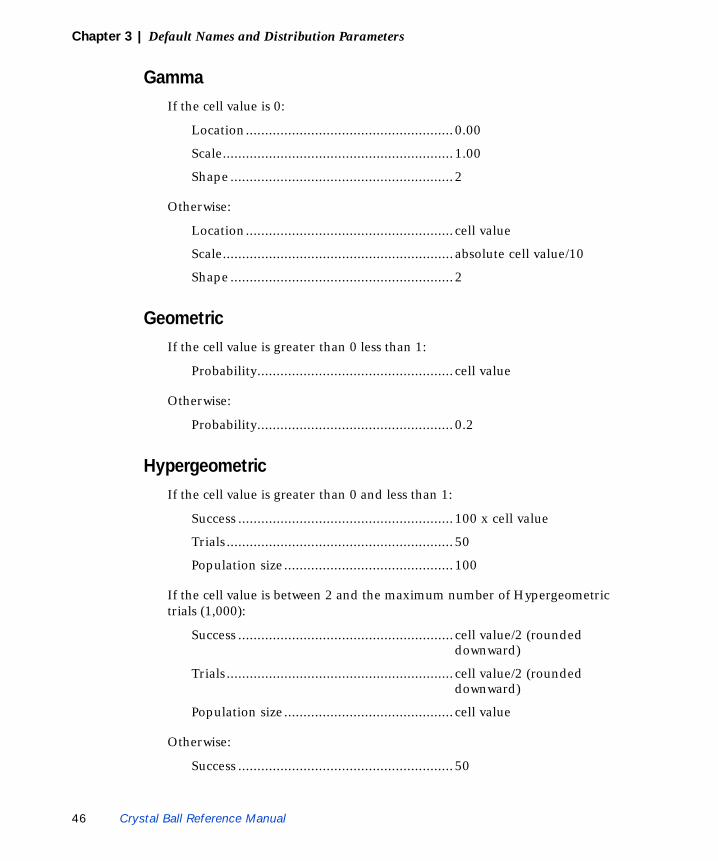
GammaIf the cell value is 0:

Location...................................................... 0.00

Scale............................................................ 1.00

Shape .......................................................... 2

Otherwise:

Location...................................................... cell value

Scale............................................................ absolute cell value/10

Shape .......................................................... 2

GeometricIf the cell value is greater than 0 less than 1:

Probability................................................... cell value

Otherwise:

Probability................................................... 0.2

HypergeometricIf the cell value is greater than 0 and less than 1:

Success ........................................................ 100 x cell value

Trials ........................................................... 50

Population size ............................................ 100

If the cell value is between 2 and the maximum number of Hypergeometric trials (1,000):

Success ........................................................ cell value/2 (rounded downward)

Trials ........................................................... cell value/2 (rounded downward)

Population size ............................................ cell value

Otherwise:

Success ........................................................ 50



Trials........................................................... 50

Population size............................................ 100

LogisticIf the cell value is 0:

Mean .......................................................... 0

Scale ........................................................... 1.0

Otherwise:

Mean .......................................................... cell value

Scale ........................................................... absolute cell value/10

LognormalIf the cell value is greater than 0:

Mean .......................................................... cell value

Standard Deviation ..................................... absolute cell value/10

Otherwise:

Mean .......................................................... e

Standard Deviation ..................................... 1.0

Maximum extreme valueIf the cell value is 0:

Likeliest ...................................................... 0

Scale ........................................................... 1

Otherwise:



Minimum extreme valueIf the cell value is 0:

Likeliest ...................................................... 0



Scale............................................................ 1

Otherwise:



Negative binomialIf the cell value is less than or equal to 0:

Probability................................................... 0.2

Shape .......................................................... 10

If the cell value is greater than 0 and less than 1:

Probability................................................... cell value

Shape .......................................................... 10

Otherwise (unless cell value > 100):

Probability (Prob) ........................................ 0.2

Shape .......................................................... cell value

If cell value > 100, Shape ........................... 10

NormalIf the cell value is 0:

Mean........................................................... 0

Standard Deviation ..................................... 1.00

Otherwise:

Mean........................................................... cell value

Standard Deviation ..................................... absolute cell value/10.0

ParetoIf the cell value is between 1.0 and 1,000:


Shape .......................................................... 2



Otherwise:

Location ..................................................... 1.00

Shape.......................................................... 2

PoissonIf the cell value is less than or equal to 0:

Rate ............................................................ 10.00

If the cell value is greater than 0 and less than or equal to the maximum rate (1,000):

Rate ............................................................ cell value

Otherwise:

Rate ............................................................ 10.00

Student’s tIf the cell value is 0:

Midpoint..................................................... 0

Scale ........................................................... 1.00

Degrees....................................................... 5

Otherwise:

Midpoint..................................................... cell value


Degrees....................................................... 5

TriangularIf the cell value is 0:

Likeliest ...................................................... 0

Minimum.................................................... -10.00

Maximum ................................................... 10.00

Otherwise:






UniformIf the cell value is 0:

Minimum .................................................... -10.00

Maximum ................................................... 10.00

Otherwise:



WeibullIf the cell value is 0:

Location...................................................... 0

Scale............................................................ 1.00

Shape .......................................................... 2

Otherwise:



Shape .......................................................... 2

Yes-NoIf the cell value is greater than 0 and less than 1:

Probability of Yes(1) .................................... cell value

Otherwise:

Probability of Yes(1) .................................... 0.5


Index

In this indexA comprehensive index designed to give you quick access to the information in this manual.


Index

Aassumptions

parameters 43

Bbeta distribution

formula 30betaPERT distribution

formula 31binomial distribution

formula 31

Ccapability metrics 20confidence intervals 18consulting 2contact information 2Cp 20Cpk 22Cpk-lower 21Cpk-upper 21Cpm 22custom distribution

formula 39

Ddiscrete uniform distribution

formula 32distributions

fitting methods 40parameter defaults 43

Eexponential distribution

formula 32

Fformulas

beta distribution 30betaPERT distribution 31binomial distribution 31custom distribution 39discrete uniform distribution 32exponential distribution 32gamma distribution 32geometric distribution 33hypergeometric distribution 33logistic distribution 34lognormal distribution 34

maximum extreme distribution 35minimum extreme distribution 35negative binomial distribution 36normal distribution 36Pareto distribution 37Poisson distribution 37precision control 18random number 19Student’s t distribution 37triangular distribution 38uniform distribution 38Weibull distribution 39

Ggamma distribution

formula 32geometric distribution

formula 33

H-Khow this manual is organized 1hypergeometric distribution

formula 33

LLatin hypercube sampling

defined 17logistic distribution

formula 34lognormal distribution

formula 34LSL 26

Mmaximum extreme distribution

formula 35maximum likelihood estimators 40mean confidence interval 19metrics

process capability 20quality 20

minimum extreme distributionformula 35

Monte Carlo simulationhistory 16

Nnaming defaults 42negative binomial distribution


1

formula 36normal distribution

formula 36

Pp(N/C)-above 25p(N/C)-below 25p(N/C)-total 26parameter defaults, assumptions 43Pareto distribution

formula 37peakedness 11percentiles confidence interval 19Poisson distribution

formula 37Pp 20Ppk 22Ppk-lower 21Ppk-upper 21Ppm 23PPM-above 26PPM-below 26PPM-total 26precision control

confidence intervals 18precision control formulas 18process capability metrics 20

Qquality statistics 20

Rrandom number formula 19

Sscreen capture notes 2Six Sigma statistics 20standard deviation confidence interval 19statistics, quality 20Student’s t distribution

formula 37support resources 2

TTarget value 27technical support 2training 2triangular distribution

formula 38

Uuniform distribution

formula 38USL 26

WWeibull distribution

formula 39

ZZ-LSL 23Zlt 24Zlt-total 25Z-score shift 27Zst 23Zst-total 24Z-USL 23


Index



Credits

Crystal Ball Reference Manual

Updated and edited by Barbara Gentry, Eric Wainwright, and David Blankinship.

Previous contributors included Carol Werckman, Terry Hardy, and Cameron Harris.

Illustrations and screen captures by Barbara Gentry using Jasc, Inc. Paint Shop Pro.

Typeset using NewBskvll BT and Univers fonts.

CB7 Reference Manual

Documents

Transcript of CB7 Reference Manual