Causality, Causal Models, and Social Mechanisms

Daniel Steel

Department of Philosophy

Michigan State University

503 S Kedzie Hall

East Lansing, MI 48824-1032

Introduction

Causation is one of the most important and contentious issues in social science. Any

aspirations for a better social world, whether they concern the alleviation of inequities or

the promotion of wealth, must explicitly or implicitly rely on beliefs about the causes and

effects of government policies, social institutions, norms, or other phenomena that fall

within the purview of social science. Yet everyday exemplars of cause and effect

relations are typically drawn from relatively simple physical setups and machines such as

billiards and lawnmowers. Indeed, the expression “social mechanism” reflects this

transfer of concepts from mechanical to social. Moreover, many important questions in

social science concern social systems and phenomena—economies, racial segregation,

etc—whose extent and complexity make them difficult if not impossible to study in

controlled laboratory settings. The result of all this is that causation is central and

perennial issue for the philosophy of social science. This chapter examines three general

approaches to studying causation in social science and the conceptual connections among

them.

One commonly drawn distinction in social science research is between

quantitative and qualitative approaches. Whereas quantitative research examines large

sets of numerical data which are then analyzed by means of statistical techniques,

qualitative research focuses in depth on a relatively small number of cases. A good

representative of the mainstream view on the relationship between these two approaches

can be found in the influential book, Designing Social Inquiry: Inference in Qualitative

Research (King, Keohane, and Verba 1994), which I will henceforth refer to as DSI.

According to DSI, a shared logic underlies both quantitative and qualitative research and

1

this logic is most clearly exhibited in quantitative research. Advocates of qualitative

research, while mostly agreeing that there are important commonalities among the two

approaches, reject what they perceive as DSI’s characterization of qualitative research as

the poor relation to quantitative social science (Ragin 2004; McKeown 2004). Charles

Ragin also critiques the “quantitative versus qualitative” distinction, arguing that the

intended contrast is better drawn in terms of variable versus case oriented research (Ragin

1987). Ragin’s formulation of this distinction associates the two approaches with distinct

types of models: linear equations for variable oriented and Boolean logic for case

oriented. I adopt the “variable versus case” version of the distinction mainly because I

find the emphasis on types of causal model fruitful. Variable oriented social science

research is also contrasted with mechanism approaches (Hedström and Swedberg 1998;

George and Bennet 2005). Mechanism approaches study causal relationships by

developing models, often represented by mathematical formula, of micro-processes that

could generate a macro-sociological phenomenon of interest. Advocates of social

mechanisms often claim that they can overcome difficulties associated with variable

oriented research, especially, the problem that a correlation found in the data may be

explained by an omitted variable rather than a direct causal influence (Elster 1983; Little

1991; Hedström and Swedberg 1998).

In this chapter, I explore the interrelationships among variable, case, and

mechanism oriented approaches to social science research. I agree that there is a

common logic behind variable and case oriented approaches, but I suggest that this

commonality is best formulated within an approach to causal inference that relies on

Bayesian networks (Bayes nets, for short). More specifically, the types of causal models

2

associated with the two approaches—linear equations for variable oriented and Boolean

logic for case oriented approaches—are two types of parameterizations of Bayes nets.

The Bayes nets framework, therefore, identifies model-general aspects of causal

inference that pertain to these two as well as other types of causal models and thereby can

reasonably be taken to articulate the “underlying logic” of causal inference to which the

author’s of DSI refer. One useful consequence of this analysis is that it shows how

challenges often associated with variable oriented approaches—such as problems linked

to omitted common causes—are also difficulties for case oriented research. Finally, I

consider the connection of mechanism-oriented research to variable and case oriented

approaches to causal inference. Advocates of mechanisms in social science typically

claim that mechanisms are valuable for explanation and for assisting causal inference. I

focus on the second of these two claims here and suggest that the relationship between

mechanism and variable oriented approaches is best understood by way of a distinction

between what I call direct and indirect causal inference.

Variable versus Case Oriented Approaches

The contrast between quantitative and qualitative social science research naturally

suggests a difference that has to do with numbers: quantitative researchers work with a

large samples of numerical data that they subject to statistical analysis, while qualitative

researchers delve into non-quantifiable features of a relatively small number of cases.

For example, this sort of distinction seems, at least to a first approximation, to capture

central differences between such social science disciplines as econometrics and cultural

anthropology. Those who pursue quantitative approaches to social sciences are more

3

likely to see their methods as continuous with natural science, while a tendency to

identify with research methods typical of the humanities is more common, though

certainly not universal, among qualitative researchers. Thus, the quantitative versus

qualitative distinction taps into an old and central debate about the nature of social

science method and it relation to methods in the natural sciences. In this section, I focus

on the positions taken on this issue in DSI and in reactions to it.

It is safe to say that DSI is the most widely discussed work on social science

methodology published in the last twenty-five years (cf. Brady and Collier 2004; George

and Bennett 2005). The central theme of DSI is that differences between quantitative and

qualitative approaches to social research are primarily matters of style rather than

substance and that both approaches rely on “the same underlying logic of inference” (p.

4). But while insisting that “neither quantitative nor qualitative research is superior to the

other” (p. 5), DSI goes on to make clear that it regards good quantitative social research

as a model for good social science in general.

non-statistical research will produce more reliable results if researchers pay

attention to the rules of scientific inference—rules that are sometimes more

clearly stated in the style of quantitative research. … The very abstract, and even

unrealistic, nature of statistical models is what makes the rules of inference shine

through so clearly. (p. 6)

The central thesis of DSI and the arguments for it have stimulated a good deal of critical

discussion among social scientists. One line of criticism stems from social scientists who

identify as qualitative or case-oriented researchers and who reject what they see as the

lack of understanding or proper respect paid to their methods by DSI. The representative

4

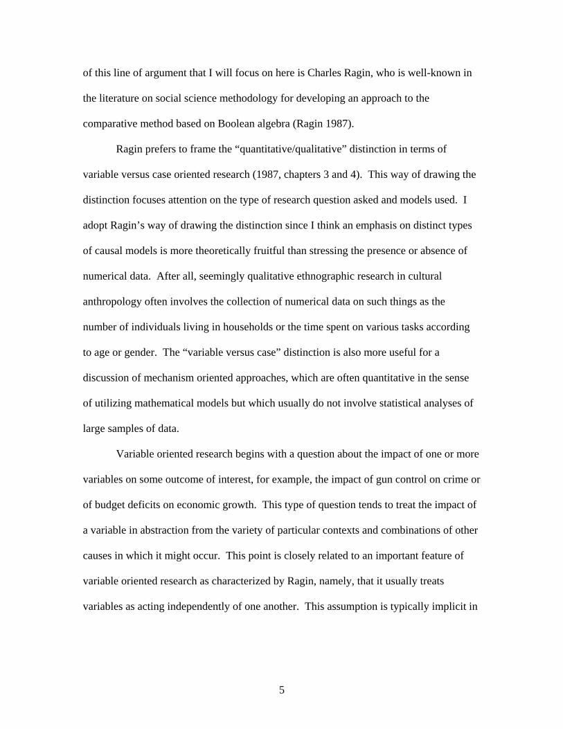
of this line of argument that I will focus on here is Charles Ragin, who is well-known in

the literature on social science methodology for developing an approach to the

comparative method based on Boolean algebra (Ragin 1987).

Ragin prefers to frame the “quantitative/qualitative” distinction in terms of

variable versus case oriented research (1987, chapters 3 and 4). This way of drawing the

distinction focuses attention on the type of research question asked and models used. I

adopt Ragin’s way of drawing the distinction since I think an emphasis on distinct types

of causal models is more theoretically fruitful than stressing the presence or absence of

numerical data. After all, seemingly qualitative ethnographic research in cultural

anthropology often involves the collection of numerical data on such things as the

number of individuals living in households or the time spent on various tasks according

to age or gender. The “variable versus case” distinction is also more useful for a

discussion of mechanism oriented approaches, which are often quantitative in the sense

of utilizing mathematical models but which usually do not involve statistical analyses of

large samples of data.

Variable oriented research begins with a question about the impact of one or more

variables on some outcome of interest, for example, the impact of gun control on crime or

of budget deficits on economic growth. This type of question tends to treat the impact of

a variable in abstraction from the variety of particular contexts and combinations of other

causes in which it might occur. This point is closely related to an important feature of

variable oriented research as characterized by Ragin, namely, that it usually treats

variables as acting independently of one another. This assumption is typically implicit in

5

choosing to represent the influences of the causes upon the effect by means of a linear

equation such as the following.

εβββα ++++= 332211 xxxy

Here y is the dependent variable (the effect), x1 through x3 are the independent variables

(potential causes), α is the intercept, β1 through β3 are the coefficients, and ε is the error

term which represents the effects of any omitted causes. For example, y might be a

variable representing income, while x1 through x3, respectively, stand for educational

attainment, IQ, and parents’ income. The research question, then, might be: what impact

do these three variables have on income? Possible answers correspond to distinct

assignments of numbers to the coefficients. To assume that the correct answer fits the

form of the above equation entails some assumptions about what the correct answer could

be, for instance, that the independent variables act separately upon y (e.g. the impact of x2

does not depend on the value of x3).

In contrast, case oriented research is motivated by an interest in one or a small

number of cases. For example, a case oriented researcher might be stimulated by an

interest to explain the bursting of the “dot-com” bubble in the late 1990s, a question that

would naturally invite comparisons with other stock market busts. A key feature of case

oriented research as understood by Ragin is that it is deeply concerned with teasing apart

complex interactions of causes found in particular cases. According to Ragin, when

pursuing a case oriented approach:

Researchers examine cases as wholes, not as collections of variables. An interest

in interpreting specific cases and in pinpointing the combinations of conditions,

6

the causal complexes, that produce specific outcomes encourages investigators to

view cases as wholes. (1987, p. 52)

Ragin’s approach is intended for cases in which causes and effects can be represented by

as conditions or events are that are present or absent. The goal, then, is to identify which

combination of conditions (or absences) result in the outcome. Boolean logic, which will

be familiar to anyone who has taken an introductory logic class, can be used to represent

relationships among variables in such circumstances. This is best understood by way of

an example. Consider the truth table in figure 1, which is adapted from Ragin (1987, p.

96). This table is a hypothetical example of a study of three potential causes of a

successful strike (S): high demand for the product produced by the striking workers (A),

threat that other workers will also go on strike out of sympathy or solidarity (B), and a

large strike fund (C). In the table, 1’s indicates that the condition is present and 0’s

indicates that it is absent. For example, in the forth row from the top, only A is present

while B, C, and S are absent.

A B C S Number of Cases 1 1 1 1 3 1 1 0 1 2 1 0 1 1 6 1 0 0 0 9 0 1 1 0 3 0 1 0 1 5 0 0 1 0 6 0 0 0 0 4

Figure 1: A hypothetical example: A = booming product market, B = threat of sympathy

strikes, C = large strike fund, and S = successful strike.

7

Given a table of this sort, Ragin describes some fairly simple procedures for

identifying sets of minimal combinations of causes that generate the outcome. First, list

the rows in the table for which the outcome S is present, which in figure 1 are the first

through third rows and the sixth row. This can be represented in the following Boolean

equation.

CBACBACABABCS ⊕⊕⊕=

In this equation, a line over a letter indicates the absence of that characteristic, for

instance, C indicates the absence of C. The ⊕ symbol is called “Boolean addition,”

which is equivalent to disjunction, that is, “or.” Adjacent letters, such as ABC, represent

“Boolean multiplication,” which is equivalent to conjunction, that is, “and.” Finally, the

equals sign represents the biconditional, which can be expressed in English as “if and

only if.” Thus, the above equation is a compact representation of the rather cumbersome

claim that S is present if and only if either A, B, and C are all present, or A and B are

present while C is absent, or A and C are present while B is absent, or A and C are absent

while B is present.

As Ragin explains, a Boolean equation like the one above can often be simplified

to an equation containing fewer terms in two steps. The first step proceeds by finding

what we can call minimizing matches. A minimizing match is a disjunction of two terms

that are the same except for one letter which is has line above in one term but not in the

other. In the equation above, there are three minimizing matches: )( CABABC ⊕ ,

)( CBAABC ⊕ , and )( CBACAB ⊕ . A minimizing match is logically equivalent to a

single term that omits the letter that varies in the pair. For example,

8

ABCABABC =⊕ )( , ACCBAABC =⊕ )( , and CBCBACAB =⊕ )( .1 Thus, the

Boolean equation above simplifies to the following.

CBACABS ⊕⊕=

The next step consists of removing terms that are redundant in the sense that any way of

making the term is true will also make one or more of the other terms true. For example,

AB can be true in two ways: ABC or CAB . Yet if it is ABC, then AC is true, and if it is

CAB , then CB is true. Notice that neither AC nor CB is redundant in this sense, for

example, if CBA , then AC is true and the other two terms are false. So after removing

the redundant term AB, we are left w

ith the following.

this example, then, AC and

CBACS ⊕=

CBIn are the “prime implicants” of S, that is to say, they are

roduct

ns

.

possible causal interactions among variables, which makes it an attractive approach for

the minimal sets of conditions that are both necessary and sufficient for that outcome.

Given a causal interpretation, this hypothetical example says that the two basic

combinations of conditions that result in a successful strike are: (1) a booming p

market and a large strike fund, and (2) threat of sympathy strikes and the absence of a

large strike fund. Of course, real examples are unlikely to be as neat and clean as this

hypothetical one. In real cases it often happens that there are some possible combinatio

of the potential causes that are not instantiated in any case, and it is also not rare that

there are cases having the same values for the potential causes but different outcomes

Causal reasoning relying on Boolean logic forces one to pay careful attention to

1 Minimization is based on the logical fact that P is logically equivalent to the disjunction P and Q, or P and not-Q. For example, if Joe has red hair, then either he has red hair and green eyes, or he has red hair and does not have green eyes. And conversely, if we know that Joe either has red hair and green eyes or he has red hair and does not have green eyes, then we know that he has red hair.

9

case or

ate

e

nce

h table

arch

t

ring

logic and differ mainly in matters of

iented research in which complexes of interacting causes are a central concern. In

contrast, an approach to causal inference that relies on linear equations will tend to

obscure such interactions. Instead, it will provide an overall estimate of the impact of

each cause that depends on the frequency with which conditions necessary for the

operation of that cause happen to be present in the population. Consequently, an estim

of this kind might provide very little information about what the impact of the caus

would be in a distinct population wherein the frequency of those interacting causes are

very different. However, the major downside of Boolean approaches to causal infere

is that they are feasible only for cases involving a relatively small number of potential

causes that can take on only a very limited number of possible values, since otherwise the

truth table will be unmanageably huge. For instance, in the hypothetical example

described above, there were only three potential causes and each potential cause had only

two possible values (present or absent). In this case, the number of rows of the trut

is 23 = 8. In general, then, the number of rows in a truth table will be nm, where n is

number of possible values per potential cause and m is the number of potential causes. It

can be easily understood, then, why Boolean approaches would not be useful for rese

questions involving quantitative variables, such as income, whose range of possible

values might be in the millions. Of course, it is possible to use statistical tests for

interaction effects in conjunction with linear models like those considered above. Bu

such tests typically focus on a few salient potential interactions, rather than conside

every possible one as a Boolean analysis would.

Let us return, then, the claim made in DSI that inferences in quantitative and

qualitative social science are based on a common

10

style. P ase”

of

e

agin,

e or

rovided that we interpret this claim by reference to Ragin’s “variable versus c

rendering of the distinction, we can see that there is at least one difference that seems to

be more than merely “stylistic,” namely, the choice of which type of causal model to use.

However, the authors of DSI would insist that the common logic to which they refer

transcends differences in the type of causal model chosen (1994, 87-9). What, then, is

this common logic? In part, the logic of scientific inference proposed in DSI consists

ideas about scientific method that are largely inspired by the writings of Karl Popper

(1959). For example, DSI insists that hypotheses should be testable, and the more

testable the better (1994, pp. 19-20). In addition, DSI echoes Popper’s strictures on th

use of ad hoc modifications to save a hypothesis from apparent refutation by data:

modifications that merely restrict the scope of application of a hypothesis, and hence

reduce its testability, are undesirable (pp. 21-22). Some critics of DSI, especially R

take issue with its stance on the use of ad hoc modifications in response to cases that

contradict a theoretical prediction (2004, p. 126). Besides its insistence on some very

general points about scientific method, DSI also gives more specific advice about

appropriate methods for testing causal hypotheses. For example, DSI stresses that causal

inference is possible only from data in which there is variation in the potential caus

causes (p. 108) as well as variation in the effect (p. 129) and that comparison groups that

differ with respect to the potential cause or causes should be relevantly similar in other

ways (pp. 91-95). Some critics take issue with the more specific recommendations about

causal inference found in DSI, particularly, with regard to the role of mechanisms in

causal inference and explanation (George and Bennett 2005, 11).

11

The focus here will be on the aspects of a common logic that pertain specifica

to causal inference rather than to scientific inference in general. In

lly

particular, I will

propose

es

w

ayesian networks (or Bayes nets, for short) are an increasingly commonly used

framework for representing r causal inference from

004).

to

that the Bayes nets approach to causation is a good candidate for a general

framework that clearly articulates a common logic of causal inference. I explain how

linear and Boolean models are simply two distinct kinds of parameterizations of Bay

nets. From this perspective, DSI is largely correct in its insistence that similar rules of

causal inference apply to variable and case oriented research. In particular, I explain ho

the possibility of unmeasured common causes—often cited as major challenge for

variable oriented research—arises for case oriented approaches as well.

Bayes Nets and Causal Models

B

causal claims and, consequently, fo

statistical data (cf. Pearl 2000, Spirtes, Glymour and Scheines 2000; Neopolitan 2

A Bayes net consists of two things: (1) a graph with arrows linking nodes that represent

variables and (2) a probability distribution over the variables in the graph. Typically,

Bayes nets approaches assume that graphs are acyclic. A graph is acyclic if there is no

chain of arrows aligned head-to-tail that begin and end with the same node. An acyclic

graph consisting of nodes linked by arrows is called a directed acyclic graph, or DAG.

An example of a DAG is provided in figure 2. This DAG represents a hypothesis

concerning the causal relationships among external threat (ET), external conflict (EC),

domestic power inequalities (DPI), and democratization (D). When a DAG is used

represent causal relationships, an arrow between two variables represents an influence

12

that is not mediated by any of the other variables in the DAG. However, the arrow doe

not specify the nature of that influence, for example, whether it makes the effect more

likely or less likely to occur. Such information is provided by the probability distribution

associated with the DAG rather than in DAG itself. Some terminology will be helpful

discussing the relationships represented in DAGs. In a DAG, a node X is said to be a

parent of another Y if there is an arrow pointing directly from X to Y. For example in

figure 1, the parents of D are ET and EC. A directed path is a sequence of nodes X

s

for

,

,

Figure 2: An example of a directed acyclic graph (Rasler and Thompson 2004, p. 885).

obey something known as the Markov condition.

f

nts.

1, …

Xn such that, for each pair Xi and Xi+1 in the sequence, Xi is a parent of Xi+1. In figure 2

ET → DPI → EC and DPI → EC → D are both directed paths. A node Y is said to be a

descendant of X if there is a directed path from X to Y. 2 In figure 2, for example, EC,

DPI, and D are descendants of ET.

ET EC

DPI D

In a Bayes net, the probability distribution associated with a DAG is assumed to

Markov Condition: Each variable in the graph is probabilistically independent o

its non-descendants conditional on its pare

2 Notice that the definition of directed path entails that any sequence containing only one node is a directed path, since in that case the requirement that each pair Xi and Xi+1 is linked by an arrow pointing directly from Xi to Xi+1 is trivially satisfied. Thus, every node in a DAG counts as a descendant of itself. This seemingly odd feature of the definitions is deliberate and facilitates the statement of the Markov condition.

13

In figur

Thus, t tically independent of DPI

ue D

ases

this

es of ET

ose

e 2, the parents of D are ET and EC, while DPI is the only non-descendant of D.

he Markov condition requires that D is probabilis

conditional on ET and EC. Intuitively, that means that, once you know the values of ET

and EC, learning the value of DPI doesn’t tell you anything more about what the val

is likely to be. A more precise understanding of what the Markov condition asserts

requires introducing a bit of probability notation, especially the concept of conditional

probability. A conditional probability is the probability of an event A among those c

in which B obtains. This is written as P(A | B) and read “the probability of A given B.”

An example of a conditional probability is the rate of unemployment among those who

have a college degree, which would presumably be lower than the rate of unemployment

in the general population. In probability theory, it is a standard convention is to use

lower case letters to denote the particular values of a variable. For instance, if X is a

variable representing height, then x might be a particular height (say, 6 feet). In the

simplest case, variables have only two values. For example, if D indicates

democratization, then the two values of D might indicate the presence and absence of

feature, which might be denoted d1 and d2, respectively. Likewise, the valu

(external threat) might be et1 and et2, indicating presence and absence of external threats,

respectively. Given this set up, the claim that democratization is less likely among th

states confronted by external threats would be expressed in probability symbols as

follows: P(D = d1 | ET = et1) < P(D = d1 | ET = et2). For convenience, the uppercase

letters representing variables are often omitted, which in this example results in the

following, more compact expression: P(d1 | et1) < P(d1 | et2).

14

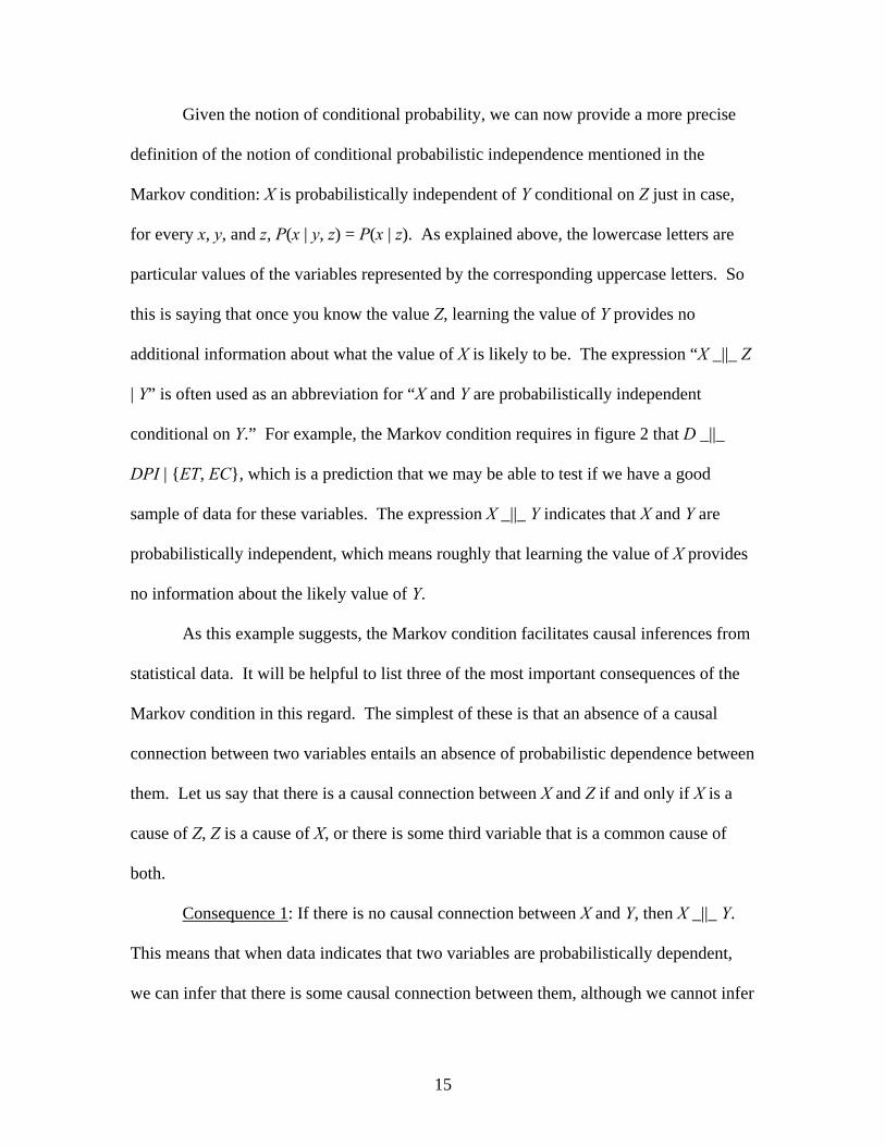
Given the notion of conditional probability, we can now provide a more prec

definition of the notion of conditional probabilistic independe

ise

nce mentioned in the

Markov

are

ides

e of the most important consequences of the

Markov

n

a

condition: X is probabilistically independent of Y conditional on Z just in case,

for every x, y, and z, P(x | y, z) = P(x | z). As explained above, the lowercase letters

particular values of the variables represented by the corresponding uppercase letters. So

this is saying that once you know the value Z, learning the value of Y provides no

additional information about what the value of X is likely to be. The expression “X _||_ Z

| Y” is often used as an abbreviation for “X and Y are probabilistically independent

conditional on Y.” For example, the Markov condition requires in figure 2 that D _||_

DPI | {ET, EC}, which is a prediction that we may be able to test if we have a good

sample of data for these variables. The expression X _||_ Y indicates that X and Y are

probabilistically independent, which means roughly that learning the value of X prov

no information about the likely value of Y.

As this example suggests, the Markov condition facilitates causal inferences from

statistical data. It will be helpful to list thre

condition in this regard. The simplest of these is that an absence of a causal

connection between two variables entails an absence of probabilistic dependence betwee

them. Let us say that there is a causal connection between X and Z if and only if X is

cause of Z, Z is a cause of X, or there is some third variable that is a common cause of

both.

Consequence 1: If there is no causal connection between X and Y, then X _||_ Y.

This means that when data indicates that two variables are probabilistically dependent,

we can r infer that there is some causal connection between them, although we cannot infe

15

from this alone whether that connection consists of one causing the other or a third

variable that is a cause of both.

Consequence 2: In both X →Y → Z and X ← Z → Y, X _||_ Y | Z. In other w

intermediate causes screen-of

ords,

f upstream causes from their effects, and common

In figur

indirec he observation that D _||_ DPI |

lds a

s

d

causes screen-off their effects from one another.

e 2, D is linked to DPI both as an effect of a common cause, ET, and as an

t effect through the path DPI → EC → D. Thus, t

{ET, EC} is an illustration of consequence 2. Combining consequences 1 and 2 yie

common strategy for drawing causal inferences from statistical data. Suppose that two

variables X and Y are correlated with one another and that we know that Y cannot be a

cause of X, for instance, because X is prior in time to Y. Then we have evidence that X i

a cause of Y if this correlation persists even when we condition on all of the possible

common cause variables that we can think of. There are some shortcomings with this

strategy—for example, some common causes might fail to be considered or a suspecte

common cause might actually be an intermediate cause. But the point here is merely to

observe that this familiar strategy presupposes the Markov condition. A third and more

surprising consequence of the Markov condition is also worthy of note.

Consequence 3: In X → Y ← Z, it is not necessarily the case that X _||_ Z | Y.

Since a node with two arrows pointing directly into it is known as a collider, this

ce.

For exa

were th

called, Y service in Vietnam, and Z whether the person was patriotic. Both X and Z are

can be restated as: conditioning on a collider can create probabilistic dependen

mple, recall the Vietnam era draft, in which men were issued draft numbers that

en randomly selected. Let X represent whether a person’s draft number was

16

causes of Y, but since X is generated by a random process, there is no causal connection

between X and Z. Nevertheless, X and Z may be dependent conditional on Y. Consid

man Joe who served in Vietnam despite the fact that his draft number was never called.

Plainly, the fact that Joe chose to go to Vietnam without being drafted will make us think

it more likely that he was patriotic way back then. In other words, among those who are

Vietnam vets, we would expect a negative correlation between being drafted and (pre-

draft) patriotism.

Let us return, then, to the variable and case oriented approaches to social research,

which as we saw tended to be associated with distinct types of causal models: linear an

Boolean equations

er a

d

, respectively. These two types of causal models are in fact distinct

types o

of

ust this

sort of approach, except with the additional assumption that all of the probabilities are 1

f parameterizations of Bayes nets. To understand what this means, it is necessary

to understand an important consequence of the Markov condition; namely, that it allows

the joint probability distribution of a set of variables to be written as the product of the

probability distribution of each variable conditional on its parents. Thus, the probability

distribution for the DAG in figure 2 can be broken down into P(ET), P(DPI | ET), P(EC |

ET, DPI), and P(D| ET, EC). However, these probabilities can be specified in a variety

distinct ways. For example, if each of the variables has only two possible values (present

or absent), then the probabilities could be given simply by indicating the probability that

the effect is present given each possible combination of values of its parents. For

example, for P(D | ET, EC), we might have P(d1 | et1, ec1) = .15, P(d1 | et1, ec0) = .35,

P(d1 | et0, ec1) = .25, and P(d1 | et0, ec0) = .75.

The Boolean equation examined in the foregoing section is an example of j

17

or 0. However, as Ragin (1987) points out, in actual case oriented research it often

happens that cases having the same combination of values for the causes do not all

exhibit

en

ble

the same outcome. In such circumstances, one could substitute a probability of

the outcome for an absolute “yes” or “no,” or perhaps code probabilities significantly less

than .5 as 0 and those significantly higher than .5 as 1. So in a Boolean approach, a

parameterization consists simply of specifying the probabilities of each variable giv

each combination of values of its parents. But as was explained in the previous section,

Boolean models are infeasible for examples involving variables—such as gross domestic

product or unemployment rate—that may take on any one of a large number of possi

values. Linear equations are a commonly used means for specifying probability

distributions in such cases. For example, suppose that D, ET, and EC each have many

possible values rather than only two. Then P(D | ET, EC) might be specified with the aid

of a linear equation like the following.

εββα +++= ecetd 21

In this case, a parameterization would consist of specifying numerical values for α, β1,

and β2, and a probability distribution for the error term ε. From a Bayes nets perspective,

then, Boolean and linear models are distinct ways of specifying a probability distribution

for a DAG.

ant facilitating condition for causal inference in variable oriented research,

since the failure of the condition may result from the presence of unmeasured common

Moreover, both approaches are consistent with the Markov condition, since the

Markov condition is satisfied in any acyclic causal model in which the error terms are

independent of one another (Steel 2005). Independent error terms are typically regarded

as an import

18

causes.

,

8,

n

that

3.

Figure 3: Boolean minimization and the Markov condition.

When unmeasured common causes are present, a natural way to proceed is to

suppose that the Markov condition holds true of a more extensive DAG in which the

omitted common causes are included (cf. Spirtes, Glymour, and Scheines 2000, chapter

6). For example, the method of instrumental variables used in econometrics (cf. Angrist

Imbens, and Rubin 1996; Lleras-Muney 2005) can be understood in this way (Steel 200

pp. 175-181). Furthermore, the minimization strategy used in conjunction with Boolea

models is a simple application of the Markov condition and of consequence 2 in

particular. Recall that Ragin’s approach to inferring causal relationships from a truth

table like that in figure 1 began by searching for minimizing matches. In a minimizing

match, a change in the value of one variable makes no difference to the outcome, or

probability of the outcome, so long as the values of the other variables remain the same.

For example, consider the relationship between the D, DPI, ET, and EC. Suppose

each of these variables have only two possible values—present and absent denoted by 1

and 0, respectively—and let P(D | ET, DPI, EC) be as represented by the table in figure

ET DPI EC D P(d1) > .51 1 1 .15 no 1 1 0 .35 no 1 0 1 .15 no 1 0 0 .35 no 0 1 1 .25 no 0 1 0 .75 yes 0 0 1 .25 no 0 0 0 .75 yes

19

In this table, once the values of ET nd are known, learning the value of DPI

makes difference to the pr bil tha is present, in other words, D _||_ DPI | {ET,

C}. Given the Markov condition, therefore, we can conclude that DPI is not a direct

cause of D. We could also formulate this table as a Boolean equation like those

onsidered in the foregoing section by coding the outcome as a “yes” or “no” depending

n whether or not the probability that D is present is greater than .5. Then an application

of Ragin’s met

a EC

oba ity t Dno

E

c

o

ECETD = , that is, Dhods would yield the Boolean equation is expected

be present when and only when both ET and EC are absent. Again, this yields the

result t

figure 3

e in

ht be

g ET

tcome

to

hat DPI does not directly impact D. In addition, interpreting Ragin’s use of

Boolean minimization in terms of Bayes nets has the significant advantage of clarifying

just what causal inferences could be justified by such an analysis and under what

circumstances. For example, one might be tempted to conclude from the table in

that DPI has no effect on D whatever. However, the table provides no basis for such an

inference because it does not rule out the possibility that DPI indirectly impacts D

through ET or EC. For example, the DAG in figure 2 predicts that D _||_ DPI | {ET, EC}

but nevertheless says that DPI → EC → D. Thus, the most we can infer from the tabl

figure 3 is that DPI is not a direct cause of D; it might be an indirect cause or it mig

no cause at all. Moreover, from the table in figure 3 alone, we cannot conclude that ET

and EC are causes of D, since the data in that table could be explained by D causin

and EC or by the existence of an unmeasured common cause. Thus, the procedures for

case-based causal reasoning recommended by Ragin are trustworthy methods for

identifying direct causes only when (1) the potential causes are not effects of the ou

variable, and (2) the outcome and potential causes are not common effects of unmeasured

20

variables.3 Of course, failures of (1) and (2) are challenges for causal inference

generally, not only for case oriented approaches. But that is merely an expectable

consequence of the fact that these challenges can be explained in terms of the Markov

condition and are independent of the particular choice of model.

The discussion in the previous paragraph relied on only consequences 1 and 2 of

the Markov condition, but not consequence 3. Recall that consequence 3 asserted

conditioning on a collider may induce probabilistic dependence. This idea is closely

related to something known as “selection bias.” Consider the following example of

selection bias provided in DSI.

Suppose we believe that American investment in third world countries is a p

cause of internal violence, and then we select a set of nations with major U.S.

investments in which there has been a good deal of interna

that

rime

l violence and another

d

in

ent.

about which nations to include in the sample is heavily

impacte

nations

that col

betwee

set of nations in which there is neither investment nor violence. (1994, p. 128)

In this example, there are three variables at play—internal violence, U.S. investment, an

inclusion in the sample—that are related as depicted in figure 4. In figure 4, inclusion

the sample is a collider, since it is an effect of both internal violence and U.S. investm

That is, the researcher’s decision

d by the values of these two variables. And as the researcher does not consider

not included in the sample, she is effectively conditioning on a single value of

lider. Hence, from consequence 3, we can infer that there may be a correlation

n internal violence and U.S. investment in her sample even if there is no causal

3 Conditions (1) and (2) are similar to J. L. Mackie’s (1974) requirement of “causal priority,” which he proposed as a qualification to his INUS theory of causation. As both Ragin’s and Mackie’s proposals are elaborations of J. S. Mill’s (1851) methods of agreement and difference, it is not surprising that the two would be confronted by similar difficulties.

21

connection between them. Notice that if there were indeed no causal connection between

internal violence and U.S. investment, then the Markov condition would entail that these

two variables would be probabilistically independent in a sample that was not subject to

selection bias.

Internal Violence

U.S. Investment

Included in Sample

Figure 4: An Example of Selection Bias.

The upshot of the discussion in this section is that a number of central points of

methodology of causal inference, such as those having to do with unmeasured common

causes and selection bias

between causality and probability arti uch

considerations, therefore, can be nsitive to the researcher’s

choice of causal model, w thing else entirely. In

contrast, some methodol ecific modeling

ssumptions. For example, the use of the method of instrumental variables to estimate a

causal e

, stem from very general considerations about the relationship

culated by the Markov condition. S

expected to be relatively inse

hether it is linear, Boolean or some

ogical considerations are closely tied to sp

a

ffect depends crucially on the assumption that causal relationships are

represented by linear equations. The main theme of this section is that Bayes nets

constitute a good framework for understanding model-general challenges for causal

22

inference and thereby can be reasonably regarded as an underlying logic of causal

inference.

Mechanisms and Causal Inference

Like case oriented researchers, advocates of social mechanisms also contrast th

approach with “variable-centered” social science (Hëdstrom and Swedberg 1998, p

17). Proponents claim that mechanisms are a needed and effective means for address

challenges that confront causal inference in social science, especially problems aris

from unme

eir

p. 15-

ing

ing

asured common causes (Elster 1983, pp. 47-8; Little 1991, pp. 24-5; Hedström

nd Swedberg 1998, p. 9). Elsewhere I have argued that mechanism proponents have not

adequately explained how eviate these genuine

f a

d

common objectives—such as a corporation, a

govern or

a

attention to social mechanisms can all

challenges for causal inference (Steel 2004). In this section, I discuss the concept o

social mechanism and then explain how, as I see it, attention to mechanisms can assist

causal inference in social science.

Mechanisms in general are characterized as sets of entities and activities

organized so as to produce a regular series of changes from a beginning state to an ending

one (Machamer, Darden, and Craver 2000). Social mechanisms in particular are usually

thought of as complexes of interactions among agents that underlie and account for

macro-social regularities (cf. Little 1991, p. 13; Stinchcombe 1991, p. 367; Schelling

1998, p. 33). The paradigm example of an agent is an individual person, but coordinate

groups of individuals motivated by

ment bureau, or a charitable organization—may also be treated as agents f

certain purposes (cf. Mayntz 2004, p. 248). Social mechanisms typically involve

23

reference to some categorization of agents into relevantly similar groups defined by a

salient position their members occupy with respect to others in the society (cf. Little

1998, p. 17; Mayntz 2004, pp. 250-2). In the description of the mechanism, the releva

behavior of an agent is often assumed to be a function of the group into which he or she

is classified. For example, consider the anthropologist Bronislaw Malinowski’s (1

account of how having more wives was a cause of increased wealth among Trobrian

chiefs. Among the Trobrianders, men were required to make substantial annual

contributions of yams to the households of their married sisters. Hence, the more wive

man had, the more yams he would receive. Yams, meanwhile, were the primary form

wealth in Trobriand society, and served to finance such chiefly endeavors as canoe

building and warfare. Although individuals play a prominent role in this account, they do

so as representatives of social categories: brothers-in-law, wives, and chiefs. The

categorization of component entities into functionally defined types is not unique to

social mechanisms. Biological mechanisms are often described using such terms as

“enzyme” and “co-receptor”. The terms “enzyme” and “co-receptor” resemble “chief”

and “brother-in-law” in virtue of being functional: all of these terms provide some

information about what role the designated thing plays in the larger system of which

a part. In sum, social mechanisms can be characterized as follows. Social mechanisms

are complexes of interacting agents—usually classified into specific social categor

that produce regularities among macro level variables.

This characterization of a social mechanism can be illustrated by another, mo

well-known example. Consider Thomas Schelling’s bounded-neighborhood model,

which is intended to account for persistent patterns of segregated housing in spite

nt

935)

d

s a

of

it is

ies—

re

24

increased racial tolerance (Schelling 1978, pp. 155-66). In this model, the residents of a

given neighborhood are divided into two mutually exclusive groups (e.g. black and

white). Each individual prefers to remain in the neighborhood, provided that the

proportion of his or her own group does not drop below a given threshold, which may

vary fro

rly,

d

ns

us

X being a cause of Y, Y being a cause of X, or the presence of some third

variabl cial

en

t to

tes

m person to person. Meanwhile, there is a set of individuals outside the

neighborhood who may choose to move in if the proportions are to their liking. Clea

this model divides individuals into groups with which characteristic preferences an

subsequent behavioral patterns are associated, and by these means accounts for macro

regularities.

Advocates of social mechanisms are motivated in large measure by concer

about the possibility that a correlation may be due to an unmeasured common cause

rather than a direct causal influence, a difficulty sometimes referred to as “spurio

correlation” (cf Elster 1983, p. 47). This was one of the general challenges for causal

inference described in the foregoing section, and it is directly tied to the fact that the

Markov condition allows that a probabilistic dependence between X and Y can be

explained by

e that is a cause of both (or any combination of these possibilities). Thus, in so

science research it is often difficult to rule out the possibility that a correlation betwe

variables is explained by a common cause that was not measured, and hence difficul

provide strong evidence of a genuine causal impact. An elucidation of underlying

mechanisms—sometimes called process tracing—is suggested by mechanism advoca

as a solution to this difficulty.

25

In order to properly understand process tracing, it is important to be clear about its

intended contrast. It is sometimes said that process tracing is utterly distinct from

methods that endeavor to draw causal inferences from statistical data. For example,

Alexander George and Andrew Bennett write that, “Process-tracing is fundamentall

different from methods based on covariance or comparisons across cases” (2005, p. 207).

Yet it is difficult to see how thi

y

s could be so if process-tracing is to enable one to

establis

fter

bitten

n

l for

h

information. Rather, the distinction is between what I call direct and indirect causal

h claims about cause and effect (Steel 2008, pp. 185-7). That is because merely

listing a sequence of contiguous events is not sufficient to demonstrate causation. A

all, how are we to know that the events in the sequence are related as cause and effect

rather than as mere coincidences? The most straightforward answer to this question is

that we distinguish between causal and coincidental sequences of events on the basis of

prior knowledge of what, in general, causes what. For example, I infer that being

by mosquitoes in Mali caused Joe’s malaria because of my belief, in general, that

mosquitoes in tropical climates are vectors of the Plasmodium protozoan that causes

malaria. But if that is right, then it seems that process tracing already assumes a solutio

to very problem that mechanism advocates claim it can solve. That is, in order to use

mechanisms to support causal inferences we already need to have a good deal of causal

knowledge.

I suggest that a more adequate explanation of how process tracing is helpfu

addressing challenges for causal inference depends on a better understanding of what

process tracing should be contrasted with. The appropriate distinction is not between one

method that relies on statistical data and another that can proceed independently of suc

26

inference. Direct causal inference attempts to infer the causal relationships among a set

of variables by examining the probabilistic relations among those same variables. By

contras

ess

es

ect

probab

ting

t, indirect causal inference attempts to learn the causal relationships among a set

of variables by examining the causal relations among a distinct yet related set. In proc

tracing, the distinct yet related variables represent features of component parts of the

larger system of interest. The usefulness of process tracing, then, rests on the possibility

that the causal relationships among the components are more directly accessible than

those among the macro-features of the system. Let us consider this idea in more detail.

Suppose that one is interested in the causal relationships among a set of variabl

V that represent macro-features of a system S. The system might be an economy, an

organism, or a machine. The variables in V might represent such things as inflation and

unemployment if S is an economy or mosquito bites and malaria if S is a person. One

strategy for learning about the causal relationships among the variables in V is by means

of statistical data concerning those variables. I call this direct causal inference (or dir

inference for short), since the strategy focuses directly on the variables of interest and the

ilistic relations among them. Direct inference can be represented schematically as

follows depicted in figure 5. For example, suppose that V contains variables represen

federal deficits, inflation, economic growth, interest rates, and unemployment. Suppose,

moreover, that the chief concern is to estimate the effect of federal deficits on economic

growth. Then direct causal inference might proceed by comparing carefully matched

periods that differ with respect to federal deficits. Attempting to infer the causal

relationships among the variables in V from statistical data concerning them together

with the Markov condition would also fall into the category of direct causal inference.

27

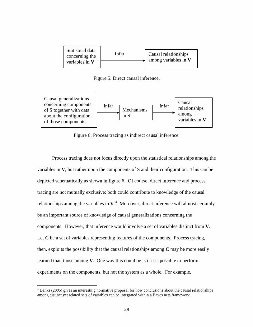
Figure 5: Direct causal inference.

Statistical data

variables in V concerning the Causal relationships

Process tracing does al relationships among the

variables in V, but rather upon the components of S and their configuration. This can be

d f course, direct inference and process

tracing are not mutually exclusive: both could contribute to knowledge of the causal

relationships among the variables in V.4 Moreover, direct inference will almost certainly

be an important so g the

omponents. However, that inference would involve a set of variables distinct from V.

Let C b

Figure 6: Process tracing as indirect causal inference.

among variables in V Infer

Causal generalizations concerning components Causal

not focus directly upon the statistic

epicted schematically as shown in figure 6. O

urce of knowledge of causal generalizations concernin

c

e a set of variables representing features of the components. Process tracing,

then, exploits the possibility that the causal relationships among C may be more easily

learned than those among V. One way this could be is if it is possible to perform

experiments on the components, but not the system as a whole. For example,

4 Danks (2005) gives an interesting normative proposal for how conclusions about the causal relationships among distinct yet related sets of variables can be integrated within a Bayes nets framework.

of S together with data about the configuration of those components

Mechanisms in S

Infer Infer relationships among variables in V

28

experimental economists can perform randomized experiments involving individuals or

small groups but not entire economies. Similarly, ethical considerations prohib

experiment in which humans are exposed to malarial mosquitoes, yet it is possible to

experimentally study, say, the transmission and action of the Plasmodium protozoan i

animal models or in vitro. Even when experiments cannot be performed on the

component parts of the system, there may be better observational data with regard

relevant features of the components than for the system as a whole, for instance

larger samples of more accurately measured data are available. Or it may be that the

possible confounders have been more exhaustively listed and measured with regard to

components than for the macro-features of the system. In short, there may be a variety

practical reasons why the causal relationships among the variables in C can be more

directly ascertained than among those in V. And when that happens, indirect inf

a reasonable approach to pursue.

Process tracing is most easily noticed in research, such as Malinowski’s study of

the Trobriand Islanders, in which data necessary for direct inference is not available, b

examples of process tracing can also be found in conjunction with direct inference. For

example, consider John Donohue and Steven Levitt’s (2001) essay, “The Impact of

Legalized Abortion on Crime.” Donohue and Levitt argue that the legalization of

abortion in the US following the 1973 Roe v. Wade decision is the most significant factor

responsible for the decline in US c

it an

n

to the

, because

the

of

erence is

ut

rime rates in the 1990s. Although it may seem

surprisi

chooses to have an abortion when the child would be unwanted, for example, because she

ng that legalizing abortion could affect crime rates two decades later, Donohue

and Levitt suggest a plausible mechanism linking the two (2001, pp. 386-9). A woman

29

would be unable to adequately care for and economically support a child or an additional

child. Donohue and Levitt cite a variety of studies that report correlations between b

raised in adverse family situations and criminality in early adulthood (2001, pp. 38

Thus, Donohue and Levitt propose that the legalization of abortion in 1973 resulted in a

birth cohort that, when entering its prime crime age 18 to 24 years later, contained

smaller proportion of individuals disposed to criminal behavior. Donohue and Levitt

give several lines of statistical evidence for this hypothesis. For example, they show tha

the drop in crime rates occurred earlier in states that legalized abortion prior to Roe v.

Wade, and that the initial decrease occurred in categories of crime disproportionately

committed by those in the 18-24 age group (2001, 395-9). Not only does Donohue and

Levitt’s study illustrate the combination between process tracing and causal inference

based on statistical data, it also illustrates the role of statistical data in process tracing

itself. For example, the causal generalization that unwanted children are more likely

become criminals is obviously a proposition that must be tested by reference to statisti

data.

Moreover, Donohue and Levitt’s study illustrates how a closer approximation o

experimental data might be attainable with regard to the mechanism than for the system

as a whole. Some studies on the effects upon criminality of being an unwanted child

focused on locations in which governmental approval was required before an abortion

was allowed, as was once the case in some parts of Scandinavia and Eastern Europe

(2001, p. 388). These studies found higher rates of criminal activity among children bor

to women who requested but were denied access to abortions than among the children of

women

eing

8-9).

a

t

to

cal

f

n

of similar socioeconomic status who did not request abortions. These studies

30

amount

ier

me

say

for

to a natural experiment involving an intervention directly on the proposed cause,

namely, access to abortion among women who desire to have one. The closest thing to a

quasi-experiment at the macro-level is Donohue and Levitt’s comparison between earl

and later legalizing states, which found that the early legalizing states (Alaska, Hawaii,

California, Washington, New York) experienced a correspondingly earlier drop in cri

rates. However, as Donohue and Levitt point out, the early legalizing states also differed

some other potentially relevant respects such as the rate of abortions after Roe v. Wade

(2001, pp. 395-396). In addition, the small number of early legalizing states and the

relatively small number of states altogether would make a statistical analysis more

tentative. Thus, this example illustrates the point made above that, for a variety of

reasons, data might allow for more firm conclusions concerning the causal relationships

at the level of mechanisms than at the level of the system as a whole. In such

circumstances, indirect inference is a reasonable approach to pursue in attempting to

establish a causal claim. Of course, it does not follow from this that process tracing

always necessary or even helpful for causal inference in social science. In some cases,

the data may support a strong conclusion on the basis of direct inference and in some

cases data needed for process tracing may be largely absent. But I think it is fair to

that process tracing, understood as indirect causal inference, is an important strategy

supporting causal conclusions in social science.

Conclusions

Learning about the causes and effects of social phenomena is an important but very

difficult task. This chapter has described three approaches to studying causation that are

31

found in social science: variable, case, and mechanism oriented research. My aim has

been to clarify the relationships among these three approaches. I suggested that variable

and case oriented research can be fruitfully considered in terms of their association with

distinct types of causal models—linear and Bool

ean equations, respectively—that

evertheless share some important features that are articulated in Bayes nets approaches

to causation. The distinction between and model-general aspects of

logic

s

-

d

Y: Rowman & Littlefield Publishers, Inc.

n

model-specific

causal inference, I propose, is a useful basis for understanding the idea that a shared

underlies these two approaches. Finally, I considered the claim that mechanisms play an

essential role in overcoming challenges to causal inference in variable and case oriented

research, such as the existence of unmeasured common causes. I suggested that this

claim is best understood by reference to what I call indirect causal inference. Tracing

mechanisms differs not in eschewing any reliance on statistical data; instead proces

tracing works by focusing attention on a distinct but related set of variables for which

better data may be available.

References

Angrist, J., G. Imbens, and D. Rubin. 1996. Identification of Causal Effects Using

Instrumental Variables. Journal of the American Statistical Association 91: 444

55.

Brady, H. and D. Collier (eds.). 2004. Rethinking Social Inquiry: Diverse Tools, Share

Standards. New York, N

32

Danks, D. 2005. Scientific Coherence and the Fusion of Experimental Results. British

Journal for the Philosophy of S 1-808.

terly

Elster, J. 1983. Explaining Technological Change: A Case Study in the Philosophy of

George n the Social

Hedströ sms: An Analytical Approach

King, G esigning Social Inquiry: Scientific Inference

Lleras- n and Adult Mortality in the

Little, D An Introduction to the Philosophy of

_____. wick, NJ:

Macham . Philosophy

Mackie University Press.

o.

cience 56: 79

Donohue, J. and S. Levitt. 2001. The Impact of Legalized Abortion on Crime. Quar

Journal of Economics 116: 379-420.

Science. Cambridge: Cambridge University Press.

, A., and A. Bennett. 2005. Case Studies and Theory Development i

Sciences. Cambridge, MA: MIT Press.

m, P. and R. Swedberg (eds.). 1998. Social Mechani

to Social Theory. Cambridge: Cambridge University Press.

., R. Keohane, and S. Verba. 1994. D

in Qualitative Research. Princeton, NJ: Princeton University Press.

Muney, A. 2005. The Relationship between Educatio

United States. Review of Economic Studies 72: 189-221.

. 1991. Varieties of Social Explanation:

Social Science. Boulder, CO: Westview Press.

1998. Microfoundation, Method, and Causation. New Bruns

Transaction Publishers.

er, P., L. Darden, and C. Craver. 2000. Thinking about Mechanisms

of Science 67: 1-25.

, J. L. 1974. The Cement of the Universe. Oxford: Oxford

Malinowski, B. 1935. Coral Gardens and Their Magic. New York: American Book C

33

Mayntz, R. 2004. Mechanisms in the Analysis of Social Macro-Phenomena. Ph

of the Social Sciences 34

ilosophy

: 237-259.

(eds.), 139-168.

Neopol tworks. Upper Saddle River, NJ: Prentice

Pearl, J and Inference. Cambridge: Cambridge

Popper

Ragin, : Moving Beyond Qualitative and Quantitative

_____. 2004. Turning the Tables: How Case-Oriented Research Challenges Variable-

Rasler, son. 2004. The Democratic Peace and a Sequential, Reciprocal,

_____. m and Swedberg (eds.),

Spirtes nd Search, 2nd

edition. Cambridge, MA: MIT Press.

McKeown, T. 2004. Case Studies and the Limits of the Quantitative Worldview. In H.

Brady and D. Collier

Mill, J. S. 1851. A System of Logic, Ratiocinative and Deductive: Being a Connected

View of the Principles of Evidence and the Methods of Scientific Investigation, 3rd

edition. London: John W. Parker.

itan, R. 2004. Learning Bayesian Ne

Hall.

. 2000. Causality: Models, Reasoning,

University Press.

, K. 1959. The Logic of Scientific Discovery. New York, NY: Routledge.

C. 1987. The Comparative Method

Strategies. Berkeley, CA: University of California Press.

Oriented Research. In H. Brady and D. Collier (eds.), 123-138.

K., and W. Thomp

Causal Arrow Hypothesis. Comparative Political Studies 37(8): 879-908.

Schelling, T. 1978. Micromotives and Macrobehavior. New York: W. W. Norton and Co.

1998. Social Mechanisms and Social Dynamics. In Heströ

32-44.

, P., C. Glymour, and R. Scheines. 2000. Causation, Prediction, a

34

Steel, D. 2004. Causal Inference and Social Mechanisms. Philosophy of the Social

Sciences 34(1): 55-78.

_____. 2005. Indeterminism and the Causal Markov Condition. British Journal for the

Philosophy of Science 56: 3-26.

2008. A_____. cross the Boundaries: Extrapolation in Biology and Social Science. New

Stinchc s

York, NY: Oxford University Press.

ombe, A. 1991. The Conditions of Fruitfulness of Theorizing about Mechanism

in Social Science. Philosophy of the Social Sciences 21: 367-88.

35