Causal Assessment Guidance Document for California Hafele Oregon Department of Environmental Quality...

Causal Assessment Evaluation and Guidance for California

Kenneth Schiff and David Gillett, Southern California Coastal Water Research Project

Andrew Rehn, California Department of Fish and Wildlife

Michael Paul, Tetra Tech, Inc.

September 2014 Technical Report 750

i

Table of Contents List of Figures ............................................................................................................................................... iii

List of Tables ................................................................................................................................................ iii

Acknowledgements ...................................................................................................................................... iv

Acronyms v

Executive Summary ....................................................................................................................................... ii

Introduction .................................................................................................................................................. 1

Objectives of this document ..................................................................................................................... 1

Causal Assessment Overview ........................................................................................................................ 3

Step 1: Defining the case .......................................................................................................................... 4

Step 2: Listing the candidate causes ......................................................................................................... 5

Step 3: Evaluating data from within the case ........................................................................................... 7

Step 4: Evaluating data from elsewhere ................................................................................................... 9

Step 5: Identifying the probable cause ................................................................................................... 10

Causal Assessment Case Study Summaries ................................................................................................ 11

Garcia River ............................................................................................................................................. 12

Case definition .................................................................................................................................... 12

List of stakeholders ............................................................................................................................. 13

Data resources and inventory ............................................................................................................. 13

Candidate causes ................................................................................................................................ 13

Likely and unlikely causes ................................................................................................................... 13

Unresolved causes .............................................................................................................................. 14

Salinas River ............................................................................................................................................ 14

Case definition .................................................................................................................................... 14






San Diego River ....................................................................................................................................... 16

Case definition .................................................................................................................................... 16

ii






Santa Clara River ..................................................................................................................................... 18

Case definition .................................................................................................................................... 18





Unresolved stressors ........................................................................................................................... 20

Important Considerations ........................................................................................................................... 21

Selecting your comparator site ............................................................................................................... 21

Evaluating data from within your case vs. data from elsewhere ........................................................... 22

Strength of inference .............................................................................................................................. 24

Data collection ........................................................................................................................................ 25

Using multi-year data .............................................................................................................................. 26

Summarizing your case ........................................................................................................................... 26

Moving past stressor identification ........................................................................................................ 27

Recommendations for Future Work ........................................................................................................... 28

Comparator site selection algorithms ..................................................................................................... 28

Species sensitivity distributions .............................................................................................................. 29

Dose-response studies ............................................................................................................................ 29

Predicting environmental conditions from biological observations ....................................................... 30

Relative risk distributions ........................................................................................................................ 31

References .................................................................................................................................................. 33

Appendix A – Garcia River Causal Assessment Case Study ........................................................................... 1

Appendix B – Salinas River Causal Assessment Case Study .......................................................................... 1

Appendix C – San Diego River Causal Assessment Case Study ..................................................................... 1

Appendix D – Santa Clara River Causal Assessment Case Study ................................................................... 1

iii

List of Figures Figure 1. Causal Assessment flow diagram in CADDIS. ................................................................................ 4

Figure 2. Conceptual diagram for increased metals as a candidate cause in the Salinas River Case Study.6

Figure 3. Example of small differences in biological condition (% collector-gatherer abundance) and larger differences in biological condition (% amphipod abundance) between test (MLS) and comparator (TWAS 1-3) sites.. .................................................................................................... 22

Figure 4. Example of using the statewide reference network for examining spatial co-occurrence. ....... 23

Figure 5. Example of using regional data for assessing stressor-response from the field. ........................ 24

Figure 6. Example species sensitivity distribution (SSD) for diazinon. ....................................................... 30

Figure 7. Example of taxon-evironmental prediction plot for different species of Cricotopus in relationship to stream bed stability. .......................................................................................... 31

Figure 8. Example of relative risk plot from the Santa Clara River case study. ......................................... 32

List of Tables Table 1. Lines of evidence based on data from within the case. ................................................................. 8

Table 2. Scoring system for spatial-temporal co-occurrence from within the case. ................................... 8

Table 3. Lines of evidence based on data from elsewhere. ......................................................................... 9

Table 4. Case study selection criteria evaluation. ...................................................................................... 11

iv

Acknowledgements The authors acknowledge the additional members of the Science Team: Scot Hagerthey U.S. Environmental Protection Agency Jim Harrington California Department of Fish and Wildlife Raphael Mazor Southern California Coastal Water Research Project Susan Norton U.S. Environmental Protection Agency Peter Ode California Department of Fish and Wildlife The authors also acknowledge the invaluable assistance of the case study participants: Lilian Busse San Diego Regional Water Quality Control Board Jenn Carah The Nature Conservancy Sarah Green Central Coast Preservation, Inc. Mary Hamilton Central Coast Regional Water Quality Control Board Ann Heil Los Angeles County Sanitation District Ruth Kolb City of San Diego Phil Markle Los Angeles County Sanitation District LB Nye Los Angeles Regional Water Quality Control Board David Paradies Central Coast Regional Water Quality Control Board Andre Sonksen City of San Diego Rebecca Veiga-Nascimento Los Angeles Regional Water Quality Control Board Jonathon Warmerdam North Coast Regional Water Quality Control Board JoAnn Weber County of San Diego Josh Westfall Los Angeles County Sanitation District Joanna Wisniewska County of San Diego Karen Worcester Central Coast Regional Water Quality Control Board The authors are grateful for the review and guidance from the Science Advisory Panel: Chuck Hawkins (Chair) Utah State University David Buchwalter North Carolina State University Rick Hafele Oregon Department of Environmental Quality (retired) Christopher Konrad U.S. Geological Survey Leroy Poff Colorado State University John Van Sickle U.S. EPA, Office of Research and Development (retired) Lester Yuan U.S. EPA, Office of Standards and Technology On the cover, clockwise from top left: Garcia River Test Site (photo credit: A Rehn); Salinas River Test Site (photo credit: S. Hagerthy); San Diego River Test Site (photo credit: D. Gillett); Santa Clara River Test Site (photo credit: D. Gillett)

v

Acronyms BMI: Benthic Macroinvertebrate

Biointegrity Policy: Biological integrity Policy being developed by the State Water Resources Control Board

CADDIS: Causal Assessment Data/Diagnostic Information System

CCAMP: CCRWQB’s Central Coast Ambient Monitoring Program

CCRWQB: Central Coast Regional Water Quality Control Board

CCWQP: Central Coast Water Quality Preservation, Inc.

CMP: CCWQP’s Cooperative Monitoring Program

CSCI: California Stream Condition Index

DFW: California Department of Fish and Wildlife

EPA: U.S. Environmental Protection Agency

EPT: ephemeroptera + plecoptera + trichoptera

GIS: Geographic Information System

IBI: Index of Biological Integrity

ICD: Interactive Conceptual Diagram

LACSD: Los Angeles County Sanitation District’s

LOEC: Lowest Effect Concentration

MLS: Mass Loading Station

MS4: Municipal Separate Stormwater Sewer System

NCRWQCB: North Coast Regional Water Quality Control Board

NorCal IBI: Northern Coastal California Benthic Index of Biotic Integrity

NPDES: National Pollutant Discharge Elimination System

PSA: Perennial Stream Assessment

POTW: Publicly Owned Treatment Works

RCMP: Reference Condition Monitoring Program

RWQCB: Regional Water Quality Control Board

SCCWRP: Southern California Coastal Water Research Project

SMC: Stormwater Monitoring Coalition

SoCal IBI: Southern California Benthic Macroinvertebrate Index of Biological Integrity

SSD: Species Sensitivity Distribution

SWRCB: State Water Resources Control Board

TMDL: Total Maximum Daily Load

TNC: The Nature Conservancy

ii

Executive Summary This document is intended for staff of regulated and regulatory agencies in California challenged with identifying the cause of degraded biological condition in streams and rivers that have been classified as impacted by the State Water Board's new biological integrity (biointegrity) policy. The goal of this document is to provide guidance to these individuals, most of whom are not biologists, on strategies and approaches for discerning the stressor(s) responsible for impacting the biological community (termed Causal Assessment). This document is not a cookbook providing step-by-step instructions for conducting a Causal Assessment, although we do provide resource information for such detailed instructions. Nor does this document supersede the need for a qualified biologist to conduct the necessary technical work. This document does provide the information for regulatory and regulated staff to understand what is necessary for conducting a proper Causal Assessment, the general framework so they know what to evaluate when selecting a contractor, and how to properly interpret the information presented in a Causal Assessment report. Finally, based on four case studies from different parts of the state, this document evaluates the US Environmental Protection Agency's Causal Analysis/Diagnostic Decision Information System (www.epa.gov/CADDIS). Associated strengths and shortcomings of CADDIS for California are presented to provide regulated and regulatory agencies a path forward for improving future Causal Assessments.

The CADDIS Causal Assessment process centers on five steps of Stressor Identification (USEPA 2000a).

1) Define the case: identify the exact biological alteration to be diagnosed at the site of impact, called the test site, including where and when. Important considerations will include what sites should be used as "comparators" for discerning differences in biology relative to changing stressor levels.

2) List candidate causes: create a list of all possible stressors that could be responsible for the biological change(s) observed. Candidate causes must be proximal (i.e., copper, pyrethroid pesticide, flow alteration, temperature, etc.); generic stressors or sources (i.e., land use type) are insufficient. For each candidate cause, a conceptual diagram (i.e., flow chart from sources to biological endpoint) should be constructed.

3) Evaluate data from the case: inventory all available biological and stressor data from test and comparator sites. Apply different lines of evidence to the data (i.e., spatial temporal co-occurrence, stressor-response, etc.) and score the results according to strength of evidence.

4) Evaluate data from elsewhere: identify data from other locations pertinent to the candidate causes including the peer-reviewed literature, nearby monitoring data from other watersheds, test and comparator site data from other time periods, etc. Apply the different lines of evidence and score the results according to strength of evidence.

5) Identify the probable causes: summarize the strength of evidence scores from the different lines of evidence for both data from within the case and elsewhere looking for consistency.

Our evaluation of CADDIS for California was positive, and we recommend its use provided stakeholders recognize its limitations. In our four test cases, we identified a subset of candidate causes, albeit with varying degrees of confidence. Equally as important, we identified several unlikely candidate causes,

iii

enabling stakeholders to bypass non-issues and focus follow-up work on candidate causes of greatest importance. However, some candidate causes were left undiagnosed when insufficient, uncertain, or contradicting evidence emerged. Subsequently, iterative steps in diagnosing and confirming candidate causes will likely result, especially where multiple stressors can result in cumulative impacts. It is clear that communication between regulated and regulatory staff will be a key to the success of any Causal Assessment, for which CADDIS is particularly well-suited.

There are at least three important considerations when adapting CADDIS to California. First is selecting appropriate comparator sites. Comparator sites are a key ingredient of the Causal Assessment approach. They enable the comparison of data relevant to candidate causes between the impacted site of interest (the test site) and a site with higher quality condition. The traditional localized (i.e., upstream-downstream) approach to selecting comparator sites met with limited success in California, largely because of the ubiquitously altered watersheds in our four test cases. However, California has a robust statewide data set encompassing nearly every habitat type in the state, which was used for developing the biointegrity numerical scoring tools including uninfluenced reference sites. This data set represents a potentially powerful tool for selecting comparator sites previously unavailable anywhere else in the nation. Future Causal Assessments should utilize the statewide data set and additional effort should focus on automating the comparator site selection process for objectively incorporating this unique resource.

Second is the distinction between evaluating data from within the case versus data from elsewhere. Data from within the case provides the primary lines of evidence for evaluating candidate causes (i.e., spatial-temporal co-occurrence, stressor-response from the field). Data from outside the case provides context for interpreting these primary lines of evidence, such as ensuring concentrations are high enough to induce biological effects (stressor-response from other field studies or from the laboratory). When comparator sites are inadequate for revealing meaningful lines of evidence from within the case, such as in our case studies from California, data from outside the case still provided the necessary information for evaluating candidate causes. Therefore, additional work to develop new assessment tools such as species sensitivity distributions, tolerance intervals, dose-response studies, relative risk distributions, or in-situ stressor-response curves will dramatically improve the utilization of data from elsewhere.

The third important consideration is summarizing the case. Oftentimes, this may be the only piece of documentation that managers will ever see. Incorporating the myriad of data analytical results for the numerous lines of evidence can be overwhelming. Narrative summary tables are used herein for our four case studies, which can be very descriptive and are consistent with CADDIS guidance. However, the narrative summaries lack much of the quantitative attributes stakeholders would prefer when making important decisions, so future efforts should develop methods or approaches for providing certainty in the diagnostic outcome.

Currently, Causal Assessments are not necessarily simple or straightforward. It must be recognized that there is a learning curve associated with implementation of any new process. As more Causal Assessments are conducted and experience gained, and new assessment tools are developed, Causal

iv

Assessments will become more efficient and informative. Ultimately, we forecast the evolution of a streamlined Causal Assessment process.

1

Introduction If you're reading this document, you likely have a perennial wadeable stream that has an impacted biological community. You might have been sampling this site for many years, or perhaps this site is new and little is known about its history, but one thing is for sure; it likely has impacted biology and is not meeting the State Water Resources Control Board's (SWRCB) biological integrity policy goals. Whether you are from a state regulatory agency such as the Regional Water Quality Control Board (RWQCB), or you are from a regulated agency such as a municipality, you're probably facing the next question. What am I supposed to do next?

One of the next important steps is to identify what is causing the biological impact, so the stream can be remediated and the biology improved to meet the biointegrity policy goals. What you need to know about biology, however, is that it's not chemistry. Chemical objectives are relatively straightforward for achieving compliance. There is typically some maximum concentration a regulated agency is not allowed to surpass. While tracking where that chemical came from can be difficult, or it may be questionable whether technology is available to reduce concentrations, compliance with traditional chemical objectives are straightforward to interpret.

Interpreting how to improve biological condition and meet biointegrity goals is much less straightforward compared to chemistry. Biological communities are dynamic and constantly changing. A biological stream sample typically comprises 11 ft2 of stream bottom and may contain thousands of organisms representing dozens of species. Each species may respond to different stressors in different ways, so a reduction in certain species is not always indicative of harm. Moreover, biological communities integrate stress over time, so an insult from months earlier may persist while the current day chemistry appears completely natural. Finally, biological communities respond to more than just chemical pollutants. For example, biological communities also respond to changes in habitat such as substrate (e.g., sand vs. cobble), temperature, hydrology, or food availability (Chessman 1999, Ode et al. in review). All of these complexities make identifying the specific cause of an impact to biological communities challenging.

Causal Assessment is the process of identifying specific stressor(s) that impact biological communities. It is precisely the complexity of biological communities and their differential response to various stressors that are exploited for deciphering the responsible stressor. It is an inexact science and, as a result, relies largely on a "weight-of-evidence" approach to either diagnose or refute a stressor. There is no single assessment tool or measurement device that can give us the answer, so we use many tools that in combination build a case towards the responsible stressor. Unfortunately, few Causal Assessments have been conducted in California. Thus, we do not know how well current approaches or assessment techniques work in our wildly varying landscapes. This limits our capability of using Causal Assessments as follow-up actions for streams that do not meet the new biointegrity goals .

Objectives of this document The objective of this document is to describe and evaluate the existing framework for conducting Causal Assessments in California for both regulated and regulatory stakeholders. We recognize that these

2

stakeholders are typically not biologists, but are faced with implementing this biologically-based regulatory policy. The goal is not to provide a step-by-step cookbook, although we do provide information about such resources. Nor does this document supersede the need for a qualified biologist to conduct the necessary technical work. Instead, our goal is to provide the strategies and approaches that will be helpful for discerning the stressor(s) responsible for the impacted biological communities. This Guidance Manual was written so that regulated and regulatory stakeholders can:

• understand the necessary steps for conducting a proper Causal Assessment,

• be knowledgeable about the Causal Assessment framework so they can properly generate a Request for Proposals or select a contractor, and

• appropriately interpret the information presented in a Causal Assessment report.

To accomplish these goals, we start with an overview of Causal Assessment and describe the framework we used. Next, we apply the Causal Assessment framework in four case studies taken from different parts of the state affected by varying land uses (urbanization, agriculture, and timber harvesting). These four case studies become the foundation for educating stakeholders using real-world examples. We then use the four case studies as the platform for insight into important considerations that stakeholders should pay attention to when conducting their own Causal Assessment. Finally, based on our case study experiences, we present the shortcomings of the Causal Assessment framework for use in California and provide regulated and regulatory agencies a path forward for improving Causal Assessment in the future.

3

Causal Assessment Overview We evaluated and the Causal Analysis/Diagnosis Decision Information System (CADDIS), an on-line decision support system supported by the U.S. Environmental Protection Agency(USEPA) to help scientists identify the stressors responsible for undesirable biological conditions in aquatic systems (http://www.epa.gov/caddis). The framework is largely based on the five steps of stressor identification (USEPA 2000a). It is arguably the most comprehensive Causal Assessment support system for degraded in-stream biological systems currently in existence.

CADDIS utilizes an inferential framework using a “weight-of-evidence” approach for determining causation, since no single line of evidence is sufficient to diagnose a candidate stressor. In many respects, moving through the CADDIS framework is akin to a prosecutor building a case against a defendant. Without an eyewitness, the case is built on several lines of evidence stacked up and pointing at the defendant (or stressor). It is also like a court case since a single, strong line of evidence can raise doubt and clear a defendant (or refute a candidate cause).

CADDIS provides a formal inferential methodology for implementation. A formal method for making decisions about causation has many benefits. First, the formal process can mitigate many of the cognitive shortcomings that arise when we try to make decisions about complex subjects. Common errors include clinging to a favorite hypothesis when it should be doubted, using default rules of thumb that are inappropriate for a particular situation, and favoring data that are conspicuous. Second, the formal process provides transparency. The need for transparency is obvious in potentially contentious regulatory settings, and CADDIS promotes open communication among interested parties. Third, CADDIS provides a structure for organizing data and a variety of data analysis tools for analyzing information. Finally, a formal method can increase confidence that a proposed remedy will truly improve environmental condition.

A full stressor identification and remediation process contains both technical and management elements (Figure 1). The technical elements focus on biological impairments and relationships to candidate causes. These relationships occur in-stream. The management aspects attribute sources to the identified cause, then develop and implement management actions to remediate and restore the biological resources. We focus on the technical aspects of Causal Assessment in this guidance document. The source attribution and mandatory regulatory requirements for remediation to achieve compliance will be determined by regulated and regulatory parties.

There are five technical elements for stressor identification in CADDIS (Figure 1). These include:

• Defining the case

• Listing the candidate causes

• Evaluating data from the case

• Evaluating the data from elsewhere

• Identifying the probable cause

http://www.epa.gov/caddis

4

The next sections briefly describe each step.

Figure 1. Causal Assessment flow diagram in CADDIS.

Step 1: Defining the case Defining the case is a scoping exercise (http://www.epa.gov/caddis/si_step1_overview.html). When completed, three basic goals will be completed: 1) defining the biological impairment; 2) defining geographic and temporal scope, and 3) selecting comparator site(s). While the Causal Assessment may be triggered by poor biointegrity, defining the exact biological impairment is fundamental. For example, the Causal Assessment trigger may be low California Stream Condition Index (CSCI) scores, but the exact biological impairment should be much more detailed. For example, loss of sensitive taxa, dominance of insensitive taxa, missing species, and absent functional groups (i.e., predators) can all capture the true nature and degree of the impairment to benthic invertebrate communities. Additional biological indicators may also be integrated as part of the causal scope including algae or fish. These additional indicators can provide valuable insight into causal confirmation and remediation requirements.

Defining the geographic and temporal scope is also an important consideration. Specificity in the location and timing of the biological impairment ensures more specific data analysis in future steps. CADDIS guidance suggests limiting your case to a single reach (e.g., test site) or a small stretch of stream with highly consistent biological condition. Assigning the test site to large areas, such as a watershed or sub-watershed, may complicate the process since more than one stressor, or single stressors at various magnitudes, can be acting in different portions of the case. Since many watersheds in California have

http://www.epa.gov/caddis/si_step1_overview.html

5

highly seasonal variability in flows, constraining seasonality to a period when biological communities are most stable will likely improve your Causal Assessment outcome.

A third element of defining the case is selecting a comparator site. A comparator site is a site, preferably within the same aquatic system (e.g., the same stream or watershed), that is either biologically unimpacted or less impacted than the test site. A comparator site does not have to be a “high-quality” reference site. If a comparator site is not a part of the same aquatic system, it is important to ensure that, aside from the influence of anthropogenic stressors, the comparator and test sites are as similar as possible in terms of natural environmental factors (e.g., elevation, size, climate, slope, and geology). Stakeholders may wish to include more than one comparator site. Additional comparator sites can be useful to help disentangle multiple stressors if the comparator sites vary in their stressor levels.

At the conclusion of this step, the Causal Assessment should have a case narrative written that defines: 1) the test site location, sampling dates, and biological effects; 2) the comparator site location, sampling dates, and biological condition relative to the test site; 3) other general descriptions or background of the watershed; and 4) objectives of the Causal Assessment project. Each of the vested regulated and regulatory agencies should read, review, and agree upon the case narrative.

Step 2: Listing the candidate causes In Step 2, the scope of the analysis is further defined in terms of the candidate causes that will be analyzed (http://www.epa.gov/caddis/si_step2_overview.html ). Rather than trying to prove or disprove a particular candidate cause, CADDIS instead identifies the most probable cause from a list of candidates. Candidate causes are the stressors that are in contact with the organisms (e.g., increased metals, habitat). Such stressors are termed Proximate Stressors. There are several strategies for compiling the list of candidate causes including reviewing available information from the site and from the region, interviewing people who have an interest in the site, and/or examining lists of candidate causes from other similar regions. CADDIS has a long list of candidate causes to help get you started (http://www.epa.gov/caddis/si_step2_stressorlist_popup.html). Selecting the appropriate list of candidate causes is a balancing act. You do not want to exclude any candidate causes that are potential stressors or that stakeholders feel strongly about. On the other hand, producing a long list of candidate causes that are superfluous will lead to a large amount of extra work or trying to make inference on candidate causes with little information. CADDIS also provides guidance on how to balance this challenge (http://www.epa.gov/caddis/si_step2_tips_popup.html ).

An important part of describing candidate causes is the construction of conceptual diagrams that describe the linkages between potential sources, stressors or candidate causes, and biological effects in the case (see Figure 2 for an example). One diagram should be developed for each candidate cause. These diagrams are developed, at least in part, to incorporate local knowledge specific to the biological impairment. The diagrams show in graphical form the working hypotheses and assumptions about how and why effects are occurring. They also provide a framework for keeping track of what information is available and relevant to each candidate cause, setting the stage for the next steps of the analysis.


http://www.epa.gov/caddis/si_step2_stressorlist_popup.html

http://www.epa.gov/caddis/si_step2_tips_popup.html

6

Figure 2. Conceptual diagram for increased metals as a candidate cause in the Salinas River Case Study.

In order to assist with developing the conceptual diagrams, CADDIS has created an Interactive Conceptual Diagram builder (ICD; http://www.epa.gov/caddis/cd_icds_intro.html). This tool will assist in understanding, describing, creating or modifying a conceptual diagram. There are a number of pre-constructed conceptual diagrams in the CADDIS library, including the conceptual diagrams developed for the four California case studies. Assuming that scientists in California build and save their conceptual diagrams to the ICD, the library will contain most conceptual diagrams important to California stakeholders in a relatively short amount of time.

While the construction of conceptual diagrams at first seems laborious, it has tremendous value in five areas. First, the conceptual diagrams help ensure there is a direct connection between a candidate

http://www.epa.gov/caddis/cd_icds_intro.html

7

cause and a biological impact. Because of the direct connection, the conceptual diagram will help control the list of superfluous candidate causes. Second, the conceptual diagrams help you to understand the dynamics of your system. When you have trouble defining the linkage between stressor and biological response, additional understanding is required. Third, the conceptual diagrams will help determine which candidate causes should be combined or separated based on their sources, fate and transformation steps, and interaction with biological components of the system. Fourth, the conceptual diagrams become a focal point for communicating between regulated and regulatory parties because each group needs to have a similar equal understanding of the processes incorporated into the diagram. Fifth, the conceptual diagram provides a guide for identifying and searching for data. Ultimately, CADDIS is trying to demonstrate the plausibility of each candidate cause by filling in the conceptual diagram boxes and arrows.

At the end of Step 2, there should be a written list of candidate causes, each with a conceptual diagram to support its linkage to the biological impacts identified in Step 1. The interaction among regulated and regulatory stakeholders in developing the list of candidate causes, and then creating the associated conceptual diagrams, will be of tremendous communication to value.

Step 3: Evaluating data from within the case CADDIS supports a wide variety of arguments and data analyses that can be used to support causal analyses (http://www.epa.gov/caddis/si_step3_indepth.html). The objective of evaluating data from within the case is to show that fundamental characteristics of a causal relationship are indeed present; for example, that the effect is associated with a sequential chain or chains of events; that the organisms are exposed to the causes at sufficient levels to produce the effect; that manipulating or otherwise altering the cause will change the effect; and that the proposed cause-effect relationship is consistent with general knowledge of causation in ecological systems.

CADDIS walks practitioners through nine different types of evidence (Table 1). Confidence in conclusions increases as more types of evidence are evaluated for more candidate causes. Although most assessments will have data for only some of the types of evidence, a ready guide to all of the types of evidence may lead practitioners to seek additional evidence.

CADDIS includes a scoring system, adapted from one used by human health epidemiologists (Susser 1986), that can be used to summarize the degree to which each type of available evidence strengthens or weakens the case for a candidate cause (http://www.epa.gov/caddis/si_step_scores.html). CADDIS provides a consistent system for scoring the evidence (Table 2), which should facilitate the synthesis of the information into a final conclusion. The number of plusses and minuses increases with the degree to which the evidence either supports or weakens the argument for a candidate cause. Evidence can score up to three plusses (+++) or three minuses (---). Alternatively, a score for NE means “no evidence” and, occasionally, the evidentiary strength is so great that a candidate cause can be assigned a “D” for diagnosed or an “R” for refuted. These scores should be entered in a standard worksheet for project accounting. After all available evidence has been evaluated; the degree to which the case for each candidate is supported or weakened is summarized.

http://www.epa.gov/caddis/si_step3_indepth.html

http://www.epa.gov/caddis/si_step_scores.html

8

Table 1. Lines of evidence based on data from within the case.

Table 2. Scoring system for spatial-temporal co-occurrence from within the case. Additional scoring tables for other lines of evidence can be found at http://www.epa.gov/caddis/si_step_scores.html.

Finding Interpretation Score

The effect occurs where or when the candidate cause occurs, OR the effect does not occur where or when the candidate cause does not occur.

This finding somewhat supports the case for the candidate cause, but is not strongly supportive because the association could be coincidental. +

It is uncertain whether the candidate cause and the effect co-occur.

This finding neither supports nor weakens the case for the candidate cause, because the evidence is ambiguous.

0

The effect does not occur where or when the candidate cause occurs, OR the effect occurs where or when the candidate cause does not occur.

This finding convincingly weakens the case for the candidate cause, because causes must co-occur with their effects. - - -

The effect does not occur where and when the candidate cause occurs, OR the effect occurs where or when the candidate cause does not occur, and the evidence is indisputable.

This finding refutes the case for the candidate cause, because causes must co-occur with their effects. R

Line of Evidence Concept

Spatial/Temporal Co-occurrence The biological effect must be observed where and when the cause is observed, and must not be observed where and when the cause is absent.

Causal Pathway Steps in the pathways linking sources to the cause can serve as supplementary or surrogate indicators that the cause and the biological effect are likely to have co-occurred.

Stressor-Response Relationships from the Field As exposure to the cause increases, intensity or frequency of the biological effect increases; as exposure to the cause decreases, intensity or frequency of the biological effect decreases.

Evidence of Exposure or Biological Mechanism Measurements of the biota show that relevant exposure to the cause has occurred, or that other biological mechanisms linking the cause to the effect have occurred.

Manipulation of Exposure Field experiments or management actions that increase or decrease exposure to a cause must increase or decrease the biological effect.

Laboratory Tests of Site Media Controlled exposure in laboratory tests to causes (usually toxic substances) present in site media should induce biological effects consistent with the effects observed in the field.

Temporal Sequence The cause must precede the biological effect.

Verified Predictions Knowledge of a cause's mode of action permits prediction and subsequent confirmation of previously unobserved effects.

Symptoms Biological measurements (often at lower levels of biological organization than the effect) can be characteristic of one or a few specific causes.

http://www.epa.gov/caddis/si_step_scores.html

9

At the end of Step 3, there should be two products: 1) a page documenting the data analytical results for each line of evidence for each candidate cause, and 2) a summary sheet scoring each line of evidence from within the case. Evaluating data from within the case provides another opportunity for interaction and communication among stakeholders. The first opportunity is compiling the data from within the case. Local stakeholders are typically the owners of this data and securing the information is critical for the success of the Causal Assessment. The second opportunity is in analyzing and interpreting the data. Communication, especially in the context of the conceptual diagrams and scoring rules, will help guide the discussion and ensure commonality in data interpretation and scoring comprehension.

Step 4: Evaluating data from elsewhere In Step 3, data from within the case is examined and scored, eliminating candidate causes from further consideration where possible and diagnosing causes using symptoms when possible. The candidate causes that remain are evaluated further in Step 4, by bringing in data from studies conducted outside of the case. The evidence developed from this information completes the body of evidence used to identify the most probable causes of the observed biological effects (Table 3).

The key distinction between data from elsewhere and data from within the case is location and/or timing: data from elsewhere are independent of what is observed at the case sites (http://www.epa.gov/caddis/si_step4_overview.html). Data from elsewhere may include information from other sites within the region; stressor-response relationships derived from field or laboratory studies; studies of similar situations in other streams, and numerous other kinds of information. This information can be collected by other monitoring programs, found in the grey literature, or compiled from the published literature. After assembling the information, it must then be related to observations from the case. As in Step 3, each type of evidence is evaluated and the analysis and results are documented in a series of worksheets. Table 3. Lines of evidence based on data from elsewhere.

Line of Evidence Concept

Stressor-Response Relationships from Other Field Studies

At the impaired sites, the cause must be at levels sufficient to cause similar biological effects in other field studies.

Stressor-Response Relationships from Laboratory Studies

Within the case, the cause must be at levels associated with related biological effects in laboratory studies.

Stressor-Response Relationships from Ecological Simulation Models

Within the case, the cause must be at levels associated with effects in mathematical models simulating ecological processes.

Mechanistically Plausible Cause The relationship between the cause and biological effect must be consistent with known principles of biology, chemistry and physics, as well as properties of the affected organisms and the receiving environment.

Manipulation of Exposure at Other Sites

At similarly impacted locations outside the case sites, field experiments or management actions that increase or decrease exposure to a cause must increase or decrease the biological effect.

Analogous Stressors Agents similar to the causal agent at the impaired site should lead to similar effects at other sites.


10

Step 5: Identifying the probable cause CADDIS uses a strength-of-evidence approach. Evidence for each candidate cause is weighed based upon data quality, accuracy of the measurements, or the data’s representativeness of the proximate stressor, and then the evidence is compared across all of the candidate causes. The evidence and scores developed in Steps 3 and 4 provide the basis for the conclusions. The strength-of-evidence approach is advantageous because it incorporates a wide array of information, and the basis for the scoring can be clearly documented and presented.

One of the challenges commonly faced by causal analyses of stream impairments is that evidence is sparse or uneven. Because information is rarely complete across all of the candidate causes, CADDIS does not employ direct comparison or a quantitative multi-criteria decision analysis approach. The scores are not added. Rather the scores are used to gain an overall sense of the robustness of the underlying body of evidence and to identify the most compelling arguments for or against a candidate cause.

At the conclusion of Step 5, there should be a summary scoring table for each candidate cause based on data from within the case and from elsewhere. A case narrative should also accompany the summary scoring table. In the best case, the analysis points clearly to a probable cause or causes. In most cases, it is possible to reduce the number of possibilities. At the least, Causal Assessment identifies data gaps that need to be filled to increase confidence in conclusions.

The next elements in the causal process are to identify sources and the management measures to remediate their biological impacts (Figure 1). This will be a critical part of the regulatory process and key to restoring biological condition. We do not address these elements in this evaluation and guidance manual. One reason we did not include source identification and management measures is because we did not conduct this part of the process in our case studies. A second reason was because abating sources and restoring biological function is by definition a site-specific task and this manual is intended to provide statewide guidance. We discuss the need for these elements in our section on Important Considerations. As additional Causal Assessments are conducted, more case studies will illustrate the success (or failures) of specific management measures. Compiling these future case studies for regulated and regulatory agencies will provide the necessary site-specific guidance on the most effective management measures to help ensure the success at restoring biological condition and achieving compliance with the state’s new bioobjectives.

11

Causal Assessment Case Study Summaries Case studies are a key component of this guidance evaluation document. They provide the opportunity to evaluate the CADDIS framework in a diverse and complex environment like California, identify the important considerations that stakeholders should pay attention to, and illuminate its limitations.

Each of the case studies was selected based on four criteria:

• Representativeness

• Stressor diversity and range of biological condition

• Data availability

• Willing partners

Representativeness focused on two perspectives; geography and landscape. We wanted the case studies to span different portions of the state and explore different land cover types such as urban, agricultural, or timber landscapes. Incorporating stressor diversity was necessary to ensure that CADDIS could accommodate a variety of candidate causes. The range of biological conditions refers to the magnitude of impacted biology, both at the test site and at the comparator sites. The biological conditions focused on benthic macroinvertebrates, composed of pre-emergent insects, worms, and gastropods (snails), since the new biointegrity policy also focuses on these organisms. Data availability is a critical element of any Causal Assessment. Like most Causal Assessments that will be conducted, we relied on existing data. For our case studies, a range of data availability was covered to assess this potential limitation. Willing partners will be an important aspect of any Causal Assessment, but testing communication between stakeholders that sometimes know each other well, and sometimes not, helped evaluate CADDIS as a bridge to effective partnership. The four case studies included: the Garcia River, Salinas River, San Diego River, and the Santa Clara River (Table 4).

Table 4. Case study selection criteria evaluation.

Watershed Geography Primary Land Cover

Range of Biological Condition

Data Availability

Willing Partners

Garcia River Northern California

Timber Good to Poor Fair RWQCB, Conservation Cooperative

Salinas River Central California Agriculture Fair to Very Poor Fair RWQCB, Agricultural Cooperative

San Diego River

Southern California

Urban Poor to Very Poor Good RWQCB, MS4

Santa Clara River

Southern California

Urban Fair to Poor Very Good RWQCB, POTW

RWQCB = Regional Water Quality Control Board; MS4 = Municipal Separate Stormwater Sewer System; POTW = Publicly Owned Treatment Works.

12

The following sections provide executive summaries from each of the case study sites outlining each of the five CADDIS Causal Assessment Steps. An important note for interpreting these summaries is that we used an Index of Biotic Integrity (IBI) (Ode et al. 2005, Rehn et al. 2005) as our trigger for evaluating the biological impact. The newest tool used for biointegrity, the California Stream Condition Index (CSCI) (Mazor et al in prep) was not fully developed when the case studies were conducted.

A detailed summary of each case can be found in Appendices A through D. These Appendices are meant to illustrate a typical Causal Assessment Report in order to provide the reader some minimum expectation of what their Report should look like. We purposely did not try to make each of the Appendices look identical. Instead, there is a common structure that users should follow, but there is a range of potential report contents for users to expect based upon data accessibility, analytical requirements, and Causal Assessment results.

Garcia River

Case definition This Causal Assessment was conducted along the inner gorge of the Garcia River that was sampled and found to be biologically impacted in 2008. The Garcia River watershed encompasses 373 km2 and flows 71 km through Mendocino County to the Pacific Ocean along the coast of northern California. Timber harvest has been the predominant land use for the last 150 years along the Garcia River. Two major waves of timber harvest occurred historically. The first wave occurred in the 1880s and was largely restricted to the lower river and its riparian zones. A second wave in the 1950s began in response to the post-World War II housing boom and the availability of better logging machinery. This second wave resulted in much of the watershed being cleared of vegetation, the construction of a vast network of roads and skid trails on steep erodible slopes, and a legacy of erosion, sedimentation, and habitat loss in stream channels that dramatically depressed native salmonid populations. The area also supported diverse farming and ranching activities before, during and between the years of timber cutting, and several thousand acres of harvested timberland were converted to range land during the 19th and early 20th centuries.

In 1993, the Garcia River was listed as impaired for elevated temperature and sedimentation per section 303(d) of the Clean Water Act. In 2002, a Sediment Total Maximum Daily Load (TMDL) Action Plan, which sought to reduce controllable human-caused sediment delivery to the river and its tributaries, was adopted into the river’s larger basin plan. Today, property owners on two-thirds of the land area in the watershed are participating in the TMDL Action Plan; half of that area (one-third of the total watershed) is managed by The Conservation Fund as a sustainable working forest (called the Garcia River Forest) with a conservation easement owned by The Nature Conservancy (TNC).

Benthic macroinvertebrate communities from the middle Garcia River in 2008 were impacted based on the Northern Coastal California Benthic Index of Biotic Integrity (NorCal IBI). Twelve sites along a 7 km section of the inner gorge had IBI scores near or below the NorCal IBI threshold of 52. Site 154 had the lowest IBI score of the 12 inner gorge sites (NorCal IBI = 36) and was defined as the test site. Two comparator sites with IBI scores above the impairment threshold were defined: Site 218 (200 m

13

downstream of Site 154) and Site 223 (1200 m upstream of Site 154). Four submetrics of the NorCal IBI were used to differentiate biological effects observed at Site 154 relative to upstream and downstream comparator sites including: 1) a decrease in EPT (Ephemeroptera + Plecoptera + Trichoptera) taxa richness; 2) a decrease in percent predator individuals; 3) an increase in percent non-insect taxa, and; 4) an increase in dominance by oligochaete worms and chironomid midges.

List of stakeholders The project partners in this Causal Assessment were the North Coast RWQCB (Jonathan Warmerdam) and the TNC (Jennifer Carah). The Science Team was led by Andrew Rehn and Jim Harrington (DFW), and included Scot Hagerthey and Sue Norton (EPA), Ken Schiff and Dave Gillett (SCCWRP), and Michael Paul (Tetra Tech).

Data resources and inventory Chemical, biological, and physical habitat data from TNC and North Coast RWQCB probabilistic monitoring programs provided the bulk of the information for data within the case during this Causal Assessment. No new data were collected. Data from elsewhere came from North Coast regional surveys conducted from 2000-2007 (n = 123 sites) and from 30 of the 56 probability sites that were sampled by TNC and RWQCB in the Garcia watershed in 2008. The latter data were included to improve applicability of regional stressor-response evaluations to the Garcia watershed and brought the total number of sites for the regional analyses to 153.

Candidate causes Sedimentation: increased embeddedness; increased sand + fine substrate

Increased Temperature: related to channel alteration, flow alteration and riparian removal

Altered Flow Regime: increased peak flow; decreased base flow; change in surficial flow

Physical Habitat: decreased woody debris, decreased in-stream habitat; change in pool/riffle frequency, increased glide habitat

Pesticides, Nutrients and Petroleum: concentrations in the water column all possibly related to illegal marijuana gardens in upper watershed. Note: specific conductivity was eventually used a surrogate variable for nutrients and pesticides

Decreased Dissolved Oxygen: related to warming, lower turbulence, increased glide habitat, increased width-to-depth ratio

Change in pH

Likely and unlikely causes Based on the available evidence, sedimentation and loss of habitat are at least partially responsible for the degraded biological community at test Site 154. In 2008, comparator sites (especially 223) were less embedded and had less sand + fines + fine gravel substrate than the case site. Greater habitat diversity was also observed at comparator sites (especially Site 223) than at the test site, including more in-

14

stream cover, more fast water (riffle) habitat, less glide habitat (case Site 154 was dominated by glide habitat in 2008), greater variation in depth, and more optimal pool-riffle frequency.

All of the inner gorge sites, including test Site 154, appear impacted by similar causal processes related to historical land use, especially road building and timber harvest, such that sedimentation and loss of habitat occurred on a watershed scale. The observed differences in sedimentation and physical habitat between the test site and comparators are consistent with causal pathways related to legacy effects from historical timber harvest/road building affecting the entire inner gorge, and Site 223 being a higher gradient, more constrained reach that transports sediment downstream and is therefore somewhat recovered physically. Stressor-response relationships between several biological metrics and sediment variables or physical habitat variables using available regional data also helped establish causal inference.

Conductivity (as a surrogate for nutrients and pesticides), changes in pH and altered flow regime were found to be unlikely contributors to poor biological condition at the case site relative to upstream and downstream comparators because observed differences in stressor values (if any) were not large enough to have ecological relevance between sites. Causal pathways linking current forestry practices or marijuana cultivation were not observed for case Site 154. Comparator sites were within close proximity, so there was little opportunity for those human activities (e.g., localized water withdrawal for irrigation of marijuana) to have a differential effect between the case site and its comparators in 2008.

Unresolved causes Longer term measurements of dissolved oxygen and temperature are needed for thorough evaluation of these candidate stressors, although certain channel alterations related to historical timber harvest contribute necessary links in causal pathways. For example, Site 154 had lower mean depth, lower pool depth, and higher width/depth ratio than comparators, which could increase average temperature. The case site also had a lower spot measurement of dissolved oxygen than the comparators and the value (6.4 mg/L) was below the minimum Coldwater standard of 7 mg/L. However, we did not wish to list lowered dissolved oxygen as a likely contributor based on a single grab sample that was collected at a different time of day than similar samples from other sites. While conductivity was used as a surrogate, no empirical data were available to allow diagnosis of nutrients, pesticides or petroleum as possible causes.

Salinas River

Case definition This Causal Assessment was conducted to determine the likely cause of biological impact at a site on the lower Salinas River, a perennial stream in an agricultural-dominated watershed located in the central coast region of California, USA. The Salinas Valley is one of the most productive agricultural regions in California. The Salinas River watershed encompasses 10,774 km2 and flows 280 km from central San Luis Obispo County through Monterey County before discharging to Monterey Bay, a National Marine Sanctuary. The river receives a variety of discharges including agricultural and urban runoff, industrial activities, and a water reclamation plant. Flow is dramatically controlled for irrigation.

15

Benthic macroinvertebrate communities in the lower Salinas River were impacted based on a Southern California macroinvertebrate Index of Biological Integrity (SoCal IBI) score less than or equal to 39 (Ode et al. 2005). This case study focused on benthic samples collected in 2006, from lower river sites at Davis Road (309DAV) and City of Spreckels (309SSP) that had SoCal IBI scores of 14 and 19, respectively. In contrast, scores were greater than 24 at the upstream comparator site near Chualar (309SAC). Four submetrics of the SoCal IBI were used to differentiate biological effects observed at the two lower Salinas River sites relative to upstream comparator sites including: 1) an increase in the percent non-insect taxa; 2) an increase in the percent tolerant taxa; 3) a decrease in percent intolerant individuals, and 4) a decrease in EPT taxa. Oligochaeta accounted for the greatest taxonomic difference, with more individuals and greater relative abundances associated with the impacted sites.

List of stakeholders The project partners for this Causal Assessment were the Central Coast RWQCB (Karen Worcester, Mary Hamilton, and David Paradise) and the Central Coast Water Quality Preservation, Inc. (Sarah Lopez). The Science Team included Scot Hagerthey and Sue Norton (EPA), Ken Schiff and David Gillett (SCCWRP), James Harrington and Andrew Rehn (DFW), and Michael Paul (Tetra Tech).

Data resources and inventory Chemical, physical, and biological data for within the case were obtained from two primary sources; the Central Coast Regional Water Quality Control Board (CCRWQB) Central Coast Ambient Monitoring Program (CCAMP) and Central Coast Water Quality Preservation, Inc. (CCWQP) Cooperative Monitoring Program (CMP). No new data was collected for this Causal Assessment. Additional significant data sources included U.S. Geological Survey daily stream flow data and the City of Salinas stormwater discharge data.

Candidate causes Decreased Dissolved Oxygen: decreased oxygen concentrations in surface water or sediments; increased dissolved oxygen fluctuations

Increased Nutrients: increased macrophyte, periphyton, phytoplankton, or microbial biomass or productivity; changes in plant assemblage structure, increased algal toxins; changes in benthic organic matter

Increased Pesticides: increased insecticides or herbicides in surface water or sediments

Increased Metals: increased membrane permeable organometallic compounds; increased metals sorbed to particles & bound to abiotic ligands

Increased Ionic Strength: increased ionic strength; increased ionic strength fluctuation; changes in ionic composition

Increased Sediments: increased eroded sediments; increased suspended sediments; increased deposited sediments; increased coverage by fines; increased embeddedness; decreased substrate size; insufficient sediment

16

Altered Flow Regime: changes in discharge patterns (magnitude and frequency); changes in structural habitat (water velocity and water depth)

Altered Physical Habitat: decreased woody debris; decreased cover; decreased bank habitat; decreased riparian habitat. Also includes the proximate stressors Increased Sediment and Altered Flow Regime.

Likely and unlikely causes Based on the available evidence, increased suspended sediments were identified as the likely cause of the biological impairment at both the Davis Rd (309DAV) and Spreckels (309SSP) sites. This diagnosis was based on greater suspended sediment concentrations at the test sites relative to comparator sites at the time of impact, supporting evidence of spatial temporal co-occurrence. Benthic macroinvertebrate responses to increased concentrations were strongly correlated and in the expected direction, supporting evidence of stressor-response from the field. Concentrations were in the range reported to cause an ecological effect, supporting evidence of stressor-response relationship from other studies. Finally, data were available to link sources to the candidate cause, supporting evidence for causal pathway. Physical habitat was also diagnosed, mostly because sediments are a component of this candidate cause. Altered flow regime was an unlikely stressor because flow regimes were similar between test and comparator sites. Decreased dissolved oxygen, increased nutrients, and increased ionic strength were unlikely stressors because there was no consistent evidence either in spatial-temporal co-occurrence or stressor response relationships, but there was less certainty in this conclusion due to data limitations. For example, dissolved oxygen was measured only during the day, possibly missing oxygen minima that would occur at night.

Unresolved causes Increased pesticides and metals were unresolved stressors due to a lack of data. Synoptic measures of these candidate stressors in water column and sediments are needed for a thorough causal assessment.

San Diego River

Case definition This Causal Assessment was conducted to determine the cause of biological impacts at a site in the lower reaches of the San Diego River in San Diego in 2010. The 1,088 km2 San Diego River watershed, located in San Diego County, passes through the heart of the City of San Diego on its way to the Pacific Ocean. The headwaters are comprised of state park and national forest open lands, and then flows 84 km through highly developed landscape in its lower reaches. San Diego has the 8th largest population in the nation, and third largest in California. Much of the lower portion has been modified for flood control. The San Diego River receives a variety of discharges including runoff from urban and agricultural land uses, industrial facilities, and a water reclamation plant. There are three major dams in the upper watershed.

Benthic macroinvertebrate communities in the lower San Diego River had a very low SoCal IBI score (7) in 2010 at the test site, a long-term monitoring site designated as the Mass Loading Station (MLS). Four upstream monitoring sites along the San Diego River (Temporary Watershed Assessment Station; TWAS 1, TWAS 2, TWAS 3, and Cedar Creek) were selected as the comparator sites. All of the sites, with the

17

exception of Cedar Creek, had poor IBI scores. To better differentiate among the test and comparator sites, four submetrics of the SoCal IBI were used: 1) % abundance of collector-gatherer taxa (e.g., Baetis spp); 2) % of non-insect taxa (e.g., oligochaetes); 3) % of tolerant taxa (e.g., Physa spp.), and; 4) % abundance of amphipods.

List of stakeholders The project partners for this Causal Assessment were the San Diego RWQCB (Lilian Busse), the City of San Diego (Ruth Kolb and Jessica Erickson), and the County of San Diego (JoAnn Weber and Joanna Wisniewska). The Science Team was led by David Gillett and Ken Schiff (SCCWRP), and included Scot Hagerthey and Sue Norton (EPA), James Harrington and Andrew Rehn (DFW), and Michael Paul (Tetra Tech).

Data resources and inventory Chemical, biological, and physical habitat data from the City and County of San Diego’s Municipal Stormwater National Pollutant Discharge Elimination System (NPDES) monitoring network provided the bulk of the information for data within the case. These data were augmented with algal community structure and sediment-bound synthetic pyrethroids data collected in 2010 at the test and comparator sites. No new data were collected. Data from elsewhere were assembled from a variety of sources including: the State of California’s Reference Condition Monitoring Program (RCMP), various probabilistic stream biomonitoring programs (e.g., Perennial Stream Assessment (PSA) and Stormwater Monitoring Coalition (SMC)), and appropriate examples from the scientific literature.

Candidate causes Altered Physical Habitat: change in available food, increase in channel deepening, decrease in the amount of riffle habitat, decrease in the amount of instream wood debris, increase in sands and fines, increase in water temperature, increase in the extent of undercut banks, increase in low dissolved oxygen, decrease in the number of cobbles, decrease in overall substrate complexity

Metals: dissolved metals, sediment-bound metals, periphyton-bound metals

Elevated Conductivity: increased total dissolved solids (TDS), increased conductivity

Increased Nutrients: change in algal community structure, increase in toxic compounds, increase in algal mat presence and thickness, increase in the frequency of hypoxia, increase in ammonia concentration

Pesticides: increased water column synthetic pyrethroids, increased sediment synthetic pyrethroids, increased “other” water column pesticides, increased “other” sediment pesticides, increased water column herbicides

Likely and unlikely causes Based on the available evidence, elevated conductivity and pesticides (specifically, synthetic pyrethroids) may be responsible for the impacted biological condition at the test site. Conductivity was a likely cause based on four lines of evidence including: 1) a clear dose response between increasing conductivity and increased amphipods and other non-insect taxa; 2) conductivity levels were high enough to degrade levels of non-insect and tolerant taxa; 3) measures of TDS across multiple months

18

illustrated a causal pathway, and; 4) the benthic community at MLS was dominated by Americorophium and Hyalella amphipods, which are indicative of saline conditions. Pyrethroid pesticides were a likely cause based on three lines of evidence including: 1) the presence of pyrethroids in the water column and sediment; 2) a relationship between synthetic pyrethroid concentrations in sediment and biological response, and; 3) few detectable measures of other non-pyrethroid pesticides. Dissolved metals in the water column were an unlikely cause based on lack of consistent metal-biological response relationships, and concentrations at the test site that were too low to generate toxicity based on studies from elsewhere. There was insufficient data to diagnose either sediment or periphyton associated metals.

Unresolved causes There was inconsistent or contradicting evidence for both nutrients and altered physical habitat from data within the case. Furthermore, there was limited data available for these candidate causes from elsewhere.

Santa Clara River

Case definition This Causal Assessment was conducted at a site in the upper reaches of the Santa Clara River located in Santa Clarita in 2006. The 4,144 km2 Santa Clara River watershed flows 134 km, starting in Los Angeles County, through Ventura County before discharging to the Pacific Ocean in the City of Ventura. The Santa Clara River is comprised of national forest in its headwaters, with mixed agricultural and urban landscapes in its middle and lower reaches. The middle and lower reaches meander through a semi-constrained floodplain, but riparian buffer extends almost to the mouth of the river. Besides the urban, agricultural, and industrial discharges, the Santa Clara River receives discharges from two water reclamation plants, with three large dams in major tributaries. Water diversions for agricultural uses are common.

Benthic macroinvertebrate communities had a low SoCal IBI score (39) in 2006 at the long-term monitoring site (designated RD) immediately downstream of the Los Angeles County Sanitation District’s (LACSD) Valencia Water Reclamation Plant outfall. Two upstream (RB, RC), two downstream (RE, RF), and three tributary sites (SAP8, SAP11, and SAP14) were selected as the comparator sites. All of the comparator sites had low SoCal IBI scores (4-34) as well. To better differentiate biological impact among the test and comparator sites, three metrics of the SoCal IBI were used: 1) % of non-insect taxa (e.g., oligochaetes); 2) % of tolerant taxa (e.g., Physa spp.); and 3) number of predator taxa.

Comparator sites were selected based largely on proximity to the test site and availability of data (detailed in Appendix D). However, the similarly poor biological condition of the test and comparator sites complicated the causal assessment, ultimately reducing confidence from lines of evidence within the case. Meaningful biological differences between test and comparator sites are necessary for deriving inference for several lines of within the case evidence including spatial-temporal co-occurrence and dose-response from the field. This emphasizes the need to select appropriate comparator sites, even if they are outside the immediate watershed.

19

List of stakeholders The project partners for this Causal Assessment were the LACSD (Phil Markle and Josh Westfall) and the Los Angeles RWQCB (Becky Vega-Nascimento and LB Nye). The Science Team was led by David Gillett and Ken Schiff (SCCWRP), and included James Harrington and Andrew Rehn (DFF), Scot Hagerthey and Sue Norton (EPA), and Michael Paul (Tetra Tech).

Data resources and inventory Chemical, biological, and physical habitat data from the LACSD NPDES monitoring programs for Valencia and Saugus outfalls provided the bulk of the information for data within the case. The main stem and tributary sites had similar data, but the tributary sites were supplemented with algal community structure and temporally intensive (24-hr) water quality data. No new data were collected for this Casual Assessment. Data from elsewhere were assembled from a variety of sources, including: the State of California’s State of California’s Reference Condition Monitoring Program (RCMP), various probabilistic stream biomonitoring programs (e.g., PSA and SMC), and from the scientific literature.

Candidate causes Habitat Simplification: change in available food, increase in channel deepening, decrease in the amount of riffle habitat, decrease in the amount of instream wood debris, increase in sands and fines, increase in the extent of undercut banks, decrease in the number of cobbles, decrease in overall substrate complexity

Metals: dissolved metals, sediment-bound metals, periphyton-bound metals

Elevated Conductivity: increased total dissolved solids (TDS), increased chloride, increased conductivity

Increased Nutrients: change in algal community structure, increase in toxic compounds, increase in water column pH, increase in the frequency of hypoxia, increase in ammonia concentration

Pesticides: increased water column synthetic pyrethroids, increased sediment synthetic pyrethroids, increased “other” water column pesticides, increased “other” sediment pesticides, increased water column herbicides

Temperature: elevated water temperature, decreased variability in water temperature

River Discontinuity: decreased recruitment, decrease in woody debris, decrease in cobbles, increase in sands&fines, burial of cobbles, increase in simplified habitat

Likely and unlikely causes Based on the available evidence, elevated conductivity was identified as a likely cause for the biological conditions at the test site. The evaluation was based upon the results from three lines of evidence including: 1) the levels of conductivity observed at RD were high enough to potentially produce the observed levels of % of tolerant taxa; 2) the conductivity at RD exceeded the conductivity at unimpacted reference sites with the same ecological setting as RD; and 3) conductivity, TDS, and hardness were elevated at the test site (RD) compared to the upstream comparator site (RB). The large sample size of

20

data from outside the case provided sufficient context between RD and ecologically similar streams to make a reasonable conclusion for elevated conductivity.

Dissolved metals, non-pyrethroid pesticides, and increased nutrients were unlikely causes of the biological impact. Dissolved metals in the water column lacked consistent metal-biological response relationships, and concentrations at the test site were too low to generate toxicity based on studies from elsewhere. There was insufficient data to diagnose either sediment or periphyton associated metals. Non-pyrethroid pesticides were unlikely causes because concentrations were not detected in the water column at the test or comparator sites. There were no data available on pyrethroid pesticides in the water column or any sediment-bound pesticides, so these candidate causes could not be properly evaluated. Increased nutrients was an unlikely cause because proximate stressors (e.g., hypoxia, acidity) were not elevated at RD relative to the comparator sites and there were inverse relationships between all of the biological endpoints and the measures of nutrient impact. For example, diel monitoring did not indicate hypoxic or acidic conditions, even during the critical nighttime conditions. However, no outside of the case data were available for nutrients, which reduced our level of confidence in the assessment of this candidate cause.

Unresolved stressors There was inconsistent or contradicting evidence for temperature, habitat simplification and river discontinuity from within the case. Furthermore, there was limited data available for these candidate causes from elsewhere.

21

Important Considerations It must be recognized that there is a learning curve, sometimes steep, associated with implementation of any new process. As more Causal Assessments are conducted and experience gained, more efficient and conclusive Causal Assessments will occur. For the uninitiated, we identified six issues that should be of primary concern when conducting your Causal Assessment. These include selecting your comparator site, evaluating data within your case vs. elsewhere, strength of inference, data collection, summarizing your case, and moving past stressor identification. Each issue is addressed in the following sections.

Selecting your comparator site Selecting your comparator site is an important consideration because your comparator site becomes the fulcrum for judging what stressors are impacting your test site. If your comparator is too similar to your test site, then you will find few stressors because there are few differences between the two sites. If your comparator site is too dissimilar from your test site, then you will find that every stressor appears different between the two sites. Thus, selecting a comparator site is a critical component of defining your case. Selecting more than one comparator site is a viable option, and may be a good way to tease apart the evidence for multiple stressors, but know that this will increase the workload.

The first and most important attribute of selecting an appropriate comparator site is to examine the biology. You will want to dig much deeper in the biological community composition than just the CSCI score, even though the CSCI score may be the reason for conducting the Causal Assessment. For example, you could examine the component indices of the CSCI such as:

• metric scores for the predictive MMI including Shannon diversity, % intolerant taxa, tolerance value, shredder taxa, clinger taxa, Coleoptera taxa, % noninsect taxa, and collector taxa; and

• species abundance with large inclusion probability scores from the O/E model.

In our case studies, because the CSCI was not yet available, we examined the component metrics of the IBI such as % grazers, % collectors and gatherers, or % predators. It is often the component metrics, or even species abundance, where the biological response to stress can best be teased apart.

A second important consideration is the magnitude of difference in biology between the comparator site and the test site. In several of our case studies, we likely had too small of a difference between our comparator and test sites (Figure 3). This was due, in part, to the widespread impact to biological communities of our heavily human-influenced watersheds. The result of insufficient difference in biology between our comparator and test sites was that we sometimes couldn't observe a strong response in the biology to increasing stress. Ultimately, this reduced our confidence in evaluating critical lines of evidence such as spatial-temporal co-occurrence or dose-response from the field. Therefore, finding differences in biological communities between comparator and test sites is an important attribute of identifying the correct candidate cause(s).

22

Figure 3. Example of small differences in biological condition (% collector-gatherer abundance) and larger differences in biological condition (% amphipod abundance) between test (MLS) and comparator (TWAS 1-3) sites. Larger differences are preferred for CADDIS, except where natural gradient may drive these differences (CC). MLS and TWAS stations are all low gradient, low elevation sites and CC was a high gradient, higher elevation site.

A third important consideration for selecting an appropriate comparator site is similarity in natural gradients. We know that natural gradients such as rainfall, slope, watershed size, and geology all play a significant role in determining what biological community will be found at a site. Using sites that differ dramatically in these natural gradients will result in biological community differences that are not attributable to anthropogenic stress (Figure 3). Therefore, you will want to select a comparator site with as similar a natural gradient as possible. Moreover, you will want to focus on sites sampled in similar seasons to account for temporal hydrologic effects found in California.

We have found that selecting a comparator site with similar natural gradients to your test site can be challenging. In our case studies, comparator sites located upstream of potential stressors were often equally impacted as our test site. This issue of similarity in natural gradients, but differences in biology and stressor exposure is so fundamental that examining a variety of comparator sites is highly recommended. Comparator sites with similar natural gradients found within the watershed, in nearby watersheds, or even statewide should be considered.

Evaluating data from within your case vs. data from elsewhere Evaluating data within and outside your case requires special consideration because generating the different lines of evidence is the yeoman's work of Causal Assessment. Do not underestimate the

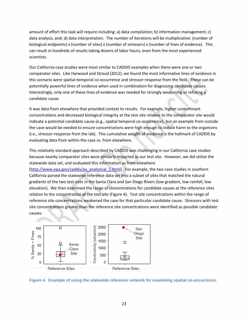
23

amount of effort this task will require including: a) data compilation; b) information management; c) data analysis, and; d) data interpretation. The number of iterations will be multiplicative: (number of biological endpoints) x (number of sites) x (number of stressors) x (number of lines of evidence). This can result in hundreds of results taking dozens of labor hours, even from the most experienced scientists.

Our California case studies were most similar to CADDIS examples when there were one or two comparator sites. Like Harwood and Stroud (2012), we found the most informative lines of evidence in this scenario were spatial-temporal co-occurrence and stressor-response from the field. These can be potentially powerful lines of evidence when used in combination for diagnosing candidate causes. Interestingly, only one of these lines of evidence was needed for strongly weakening or refuting a candidate cause.

It was data from elsewhere that provided context to results. For example, higher contaminant concentrations and decreased biological integrity at the test site relative to the comparator site would indicate a potential candidate cause (e.g., spatial temporal co-occurrence), but an example from outside the case would be needed to ensure concentrations were high enough to induce harm to the organisms (i.e., stressor-response from the lab). This cumulative weight-of-evidence is the hallmark of CADDIS by evaluating data from within the case vs. from elsewhere.

This relatively standard approach described by CADDIS was challenging in our California case studies because nearby comparator sites were similarly impacted as our test site. However, we did utilize the statewide data set, and evaluated this information as from elsewhere (http://www.epa.gov/caddis/ex_analytical_1.html). For example, the two case studies in southern California parsed the statewide reference data set into a subset of sites that matched the natural gradients of the two test sites in the Santa Clara and San Diego Rivers (low gradient, low rainfall, low elevation). We then examined the range of concentrations for candidate causes at the reference sites relative to the concentration at the test site (Figure 4). Test site concentrations within the range of reference site concentrations weakened the case for that particular candidate cause. Stressors with test site concentrations greater than the reference site concentrations were identified as possible candidate causes.

Figure 4. Example of using the statewide reference network for examining spatial co-occurrence.

http://www.epa.gov/caddis/ex_analytical_1.html

24

A similar approach was taken for evaluating stressor response relationships. Sites from a regionwide data set were parsed from the north coast within a range of natural gradients observed at the Garcia River test site. Relationships were plotted between stressor magnitude and biological response (Figure 5) and the test site fell near the bottom of the curve. These data indicate that the test site could be responding to the test site stressor.

Figure 5. Example of using regional data for assessing stressor-response from the field.

In both of these case study examples, one from southern and one from northern California, the large-scale data set provided information that offset the insufficient biological contrast between the local comparator site and impaired site. In addition, since these large-scale datasets encompass a larger range of natural variability so they are less prone to false positive (or false negative) conclusions.

We found several other assessment tools provided additional perspectives for confirming a diagnosis. The types of tools we found most useful included species sensitivity distributions (stressor response from the lab), relative risk curves (stressor response from other field studies), or tolerance intervals (stressor response from other field studies). Ideally, these objective assessment tools once developed will be stand-alone, based on the most recent information, and designed for our habitats. Once calibrated and validated, these tools can be used by any Causal Assessment in California as part of the technical toolbox.

Strength of inference Uncertainty is a fact of life. You will undoubtedly realize this as you finish your Causal Assessment. It is rare that you will have data to evaluate every line of evidence for every candidate cause. You will likely have many data gaps, including no data at all for some candidate causes. Don’t let this deter you. We recommend you follow through on what information you do have, since the Causal Assessment can eliminate candidate causes even if a diagnosis cannot be achieved.

25

The CADDIS framework incorporates uncertainty at two levels. First is at the single line of evidence where we have developed scoring rules that let you incorporate uncertainty associated with measurements. For example, the Salinas River case study created a scoring rule that downgrades a diagnosis from “+” to “O” for sites that were within measurement error. In addition, we used (and encourage others to use) important notations on uncertainty in these single line of evidence scoring tables.

The second level of uncertainty is at the summary scoring table, when one is combining lines of evidence. A new line of evidence is created within CADDIS at this stage called “consistency of evidence”. Consistency can be used to infer confidence in the diagnosis. We also found notations useful in the summary table. For example, the Garcia River case study found somewhat consistent evidence for physical habitat alteration, but not all of the indicators for physical habitat showed large differences between our test and comparator sites. We then qualified this “+” diagnosis in our summary scoring table as “weak”. These textual cues can help when combining across the potentially vast number of results generated during your data analysis.

Ultimately, we have found that the strength of evidence required to generate management actions is likely proportional to the amount of action required. If the management action is small or inexpensive, uncertainty plays a smaller role. For example, if it turns out that simple “housekeeping” is required at an industrial facility, such as sweeping instead of hosing down surfaces, then these management measures occur rapidly. However, if the action is an expensive new treatment system, increased certainty is appropriate and iterative approaches to Causal Assessment are encouraged.

The concept of iterative Causal Assessments to ensure certainty for expensive, large-scale remediation efforts reinforces one of the key values of CADDIS. This key value is communication. Our guidance strongly encourages interaction among regulated and regulatory parties. This communication occurs at several points along the Causal Assessment process including the case definition, preparing the list of candidate causes, interpreting data from within the case and elsewhere, and the conclusions based on the diagnosis. It is the early and continual interaction among decision makers that will build the consensus on whether management actions should move forward and, if not, what iterative steps will be required to build the confidence that an action should occur.

Data collection There is a tremendous amount of biological data collected in California, perhaps hundreds of sites each year. However, only a subset can be effectively used for Casual Assessment because little more than biological information is collected. Causal Assessment requires stressor data in addition to the biological data and to have the stressor data collected during the appropriate time frame. For example, the Garcia River case study had no data for nutrients to support a diagnosis. The Salinas River case study had the necessary data for pesticides and metals, but could not use them for diagnosis because water column and sediment data were not within the same temporal period as the biological assessment. Simple modifications to monitoring requirements such as when and where samples are collected as part of existing programs can yield more informative Causal Assessments. Similarly, we recommend that data generators utilize the Statewide Ambient Monitoring Program tools for data collection and

26

management. This resource will help ensure taxonomic quality and consistency (www.SAFIT.org), Standard Operating Procedures and training (http://www.waterboards.ca.gov/water_issues/programs/swamp/tools.shtml#methods), and data base consistency and access (www.CEDEN.org).

Using multi-year data Traditional CADDIS guidance recommends defining the case as a specific time period, most often a single sampling event. However, monitoring in California may have data points from multiple time periods, especially for routine NPDES monitoring. Multiple years of data collection were observed in the Salinas, San Diego, and Santa Clara River case studies. Be grateful, these data can be very useful. How to use these additional data becomes the choice of the data analyst after consultation with stakeholders and should be described in the case definition.

Data from additional time periods can be used either within the case or outside the case as data from elsewhen (as opposed to elsewhere). Utilizing the additional information as data from elsewhen is relatively straightforward and will follow the same process as data from elsewhere. Utilizing the multiple time periods as data within the case will require special caution and consideration. Merging additional time periods assumes that the stressor for each time period remains the same, and that the biological response to that stressor also remains constant.

Since CADDIS does not provide guidance on how to utilize multiple years of data within the case, we performed exploratory analysis on the Santa Clara River, which had annual biological monitoring for five years (2006-2010) and proximate stressor monitoring at even more frequent intervals. Several approaches to multi-year data analysis were evaluated including averaging across years, examining data distributions between years, and evaluating frequency of occurrence among years. In the Santa Clara case, the different approaches provided similar results and these results mirrored the likely and unresolved candidate causes from only using a single year of data (2006). Ultimately, data from additional time periods at the test site should help to provide confidence in the causal assessment regardless if the data are used within or outside the case.

Summarizing your case Summarizing your case is an important consideration because it may be the only piece of documentation that others may see. You may need to combine hundreds of analyses into an extremely brief synopsis. So, how does one do this? CADDIS recommends using narratives that follow the weight of evidence. We have used this approach in all of our case studies.

Narratives have tremendous value. They can quickly provide the snapshot that tables do not, especially to non-scientists. CADDIS prefers text because the scores given to the different pieces of evidence are not additive. In fact, one very strong piece of evidence may be sufficient to refute a candidate cause. Moreover, equivalency in the amount of data is rarely uniform, so uniform scoring tools become problematic. Text also has value because it incorporates the judgment of qualified scientists that stand-alone algorithms would not recognize.

http://www.safit.org/

http://www.waterboards.ca.gov/water_issues/programs/swamp/tools.shtml#methods

http://www.ceden.org/

27

Narratives also have drawbacks. The qualitative nature of narratives introduces the potential for bias, either in the text or in the reader’s interpretation, creating a compelling story that conveys more confidence than it deserves. Quantitative scoring systems are an alternative. For example, a Causal Assessment conducted in the Dry Creek Watershed (Washburn et al. in prep), adapted a numerical scoring system for judging lines of evidence. This algorithm included numerical rankings for strength of evidence (e.g., magnitude of concentration) for each candidate cause. This ranking was then weighted based on uncertainty (e.g., quantity of data). The quantitative summary also included commentary to supplement the scoring.

Quantitative scoring summaries may be an area of future Causal Assessment development, especially as more types of evidence become available for more stressors. Where evidence remains sparse and uneven across stressors, quantitative approaches will be difficult to implement. At least for now, we recommend sticking with CADDIS guidance to use thoughtful, objectively developed narratives based on the weight of evidence.

Moving past stressor identification Once a Causal Assessment is completed and a candidate cause has been diagnosed, the next step is to identify sources for reduction and/or elimination. We do not make recommendations for this step, since each case will be different and the regulatory decisions will be made locally. However, we recognize that source attribution is implicit in the Causal Assessment process, such as source terms in the conceptual diagrams. Because of its importance, we reference two other studies to serve as useful illustrations. The first study (Jellison et al. 2007) initiated their Causal Assessment with a specific source in mind, collecting data to either diagnose or refute the stressors associated with that source. In this study, few other sources existed so the approach was very effective for stressor confirmation. A second study (Washburn et al. in prep, http://oehha.ca.gov/ecotox.html) identified a common stressor among many sites (excess sediment), and then utilized geographic information systems (GIS) to track sources at the watershed scale. This “landscape scale” approach to source attribution was helpful for discerning patterns in biological disturbance and highlighting potential remediation pathways. These are only two cases of opposite extremes, but illustrate the range of approaches to source identification and attribution, and illustrate the reason we do not recommend any single approach. This task should be in the hands of the local regulatory and regulated agencies, which once again highlights the value of CADDIS for communication.

http://oehha.ca.gov/ecotox.html

28

Recommendations for Future Work While we recommend CADDIS for Causal Assessment, it is not perfect. Particularly for use in California, there are several shortcomings that, if addressed, will improve the quality and speed of Causal Analysis, while at the same time reducing the overall cost and uncertainty in the results. These recommendations fall into two broad categories: comparator site selection algorithms and development of new assessment tools. New assessment tools can take several forms including species sensitivity distributions, tolerance intervals, dose-response studies, relative risk distributions, and in-situ stressor response curves. Regardless of type, each of these new tools is meant to quickly compare the response of organisms at your test site to the response of organisms to individual stressors. These tools would be powerful for Causal Assessment as quick and quantitative data from elsewhere. The following sections summarize the need and utility of each data gap.

Comparator site selection algorithms In the previous section, we described the critical importance of finding the appropriate comparator site. The comparator site is the fulcrum for judging if a stressor is related to the biological response. The optimal comparator site will have similar natural gradients as the test site such as rainfall, slope, watershed size and geology. The comparator site will only differ from the test site in biological community and stressor exposure. However, we found that identifying this optimum comparator site was difficult, particularly in our ubiquitously human-influenced watersheds.

To overcome this difficulty in selecting an optimal comparator site, we recommend developing a site selection algorithm. This algorithm would highlight the important attributes for site selection, establish boundaries of natural gradients, and test for differences in biological condition and stressor status. This algorithm could even be automated and made available as an online application.

The key element of this algorithm is the use of alternative data sets. Most Causal Assessments will focus locally and typically only on the data set generated by the stakeholders at the table. These data sets may be insufficient. As we developed our case studies, it became clear that California has a robust statewide data set replete with hundreds of sites covering virtually every natural gradient. The statewide data set contained sites with rainfall ranging from <3 to 200 inches per year, sites with slopes ranging from <1 to 30 percent, sites with watershed sizes ranging from 1 to 41,000 km2, and sites covering at least nine different types of geology. This robust statewide data set becomes an invaluable resource for selecting comparator sites that most local stakeholders may have little knowledge or access.

The technology to develop an automated comparator site selection algorithm is currently available and could be completed within one year. Simply by inputting the natural gradient information from the test site, the algorithm would be compared to thousands of sites in the statewide data base. Given the criteria for an optimized comparator site, the algorithm could first search for locations within the test site watershed. If none are found, expand to nearby watersheds within the ecoregion. The algorithm could also be integrated with biological or stressor comparison modules. This objective approach to selecting comparator sites will not only save time, but will provide the most defensible Causal Assessment results.

29

Species sensitivity distributions Species sensitivity distributions (SSD) have been used for decades as a regulatory tool. SSDs are the underpinning for establishing water quality criteria used by the USEPA and adopted by the State of California (Cal Toxics Rule 2000; USEPA 2000b). Simply described, the response of various species (usually as lowest effect concentrations; LOEC) to specific toxicants are plotted against increasing concentration and then fitted with a logistic regression (Figure 6). In Causal Assessment terms, this line of evidence from elsewhere is called stressor-response relationships from laboratory studies. If the toxicant concentrations at your test site are below the range of concentrations that result in species response, that toxicant is likely not a candidate cause. In contrast, if the concentrations at your test site are in the range where most species would respond, then it might be a candidate cause. In theory and in application, the SSD is a relatively straightforward tool that can be an extremely effective line of evidence.

We recommend that SSDs be developed for more toxicants. In our case studies, we lacked SSDs for many organic contaminants including commonly used pesticides. Even for those SSDs that did exist, most lacked toxicity dosing information for important west coast species. The technology to develop this tool currently exists. Much of this information is contained within state or federal databases (i.e., ECOTOX or CalTOX) or can be found in the literature. Where the information does not exist, conducting the dosing studies is simply a matter of investment rather than technical method development. This tool could be developed in a relatively short amount of time ranging from months to years. To illustrate this point, a preliminary SSD for diazinon was developed (Figure 6); however, before such a tool can be used for assessment, a much more rigorous analysis, including verification, is needed.

Dose-response studies Dose response studies are an effective line of evidence for demonstrating the potential of a candidate cause to impart impairments. This can be done as data within the case, such laboratory toxicity tests with site water. Dose-response evidence can also arise from elsewhere, such as examining relationships between stressors and responses at other sites with similar natural gradients. In either approach, you are determining if your test site lies within the expected response (e.g., Figure 4).

The major limitation to most dose-response studies is that they rely on whole organism, single species tests. New approaches can detect dose-response information at sub-cellular through whole community levels of biological organization. For example, dosing studies are being conducted on invertebrates looking for genetic responses (Poynton et al. 2008). Not only does the activation (or de-activation) of certain genes indicate exposure to stressors, but depending on the array of observed gene responses you have the potential to deduce the offending stressor. Scientists are now determining the physiological responses of stream invertebrates to stressors, presenting the opportunity for specifying meaningful stressor levels (Buchwalter and Luoma 2005). Likewise, dose-response studies at community levels based on micro- or mesocosm studies illustrate shifts in community structure that often do not match the response of individual species. What is most promising is that all of these new approaches can not only help deduce the candidate cause, but can do so at a level of sensitivity greater than standardized whole organism acute or chronic assays.

30

We recommend exploring these new technologies for assessing dose-response. The power of these new approaches is that based on a small number of samples, one can make strong inference based on evidence from the resident organisms. However, many of the studies to date have not targeted the stressors of interest in California or have not focused on California fauna. These approaches rely on a library of responses, based on dosing from a variety of toxicants either alone or in combination. The challenge, therefore, is to create the library so that future Causal Assessments may benefit. As a result, this tool will be a challenge to create and likely take some time, but the resulting benefit would also be immensely large.

Figure 6. Example species sensitivity distribution (SSD) for diazinon. Note that the concentrations at the Salinas River test site (309SSP) were well below those for the most sensitive taxa responses, weakening the evidence for this pesticide. This SSD is considered preliminary, and its purpose is to illustrate the existence of data needed to rigorously develop defensible SSDs.

Predicting environmental conditions from biological observations Similar to tolerance intervals (Yuan 2006, Carlisle et al. 2007), Predicting Environmental Conditions from Biological Observations (PECBO) is an important module of CADDIS that could greatly expand the use of Verified Predictions as an additional line of evidence for California. In PECBO, taxon-environment

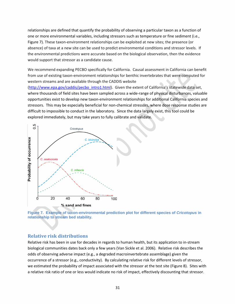
31

relationships are defined that quantify the probability of observing a particular taxon as a function of one or more environmental variables, including stressors such as temperature or fine sediment (i.e., Figure 7). These taxon-environment relationships can be exploited at new sites; the presence (or absence) of taxa at a new site can be used to predict environmental conditions and stressor levels. If the environmental predictions were accurate based on the biological observation, then the evidence would support that stressor as a candidate cause.

We recommend expanding PECBO specifically for California. Causal assessment in California can benefit from use of existing taxon-environment relationships for benthic invertebrates that were computed for western streams and are available through the CADDIS website (http://www.epa.gov/caddis/pecbo_intro1.html). Given the extent of California’s statewide data set, where thousands of field sites have been sampled across a wide-range of physical disturbances, valuable opportunities exist to develop new taxon-environment relationships for additional California species and stressors. This may be especially beneficial for non-chemical stressors, where dose response studies are difficult to impossible to conduct in the laboratory. Since the data largely exist, this tool could be explored immediately, but may take years to fully calibrate and validate.

Figure 7. Example of taxon-environmental prediction plot for different species of Cricotopus in relationship to stream bed stability.

Relative risk distributions Relative risk has been in use for decades in regards to human health, but its application to in-stream biological communities dates back only a few years (Van Sickle et al. 2006). Relative risk describes the odds of observing adverse impact (e.g., a degraded macroinvertebrate assemblage) given the occurrence of a stressor (e.g., conductivity). By calculating relative risk for different levels of stressor, we estimated the probability of impact associated with the stressor at the test site (Figure 8). Sites with a relative risk ratio of one or less would indicate no risk of impact, effectively discounting that stressor.

http://www.epa.gov/caddis/pecbo_intro1.html

32

Sites with a relative risk ratio greater than one would imply enhanced risk, increasing proportionally with the size of the ratio, strengthening the argument for that candidate cause.

The primary reason relative risk distributions are recommended in this Guidance Document is because, although they have not been fully explored in California, they could be a powerful objective assessment tool for evaluating cause. This tool could be valuable for both chemical and non-chemical stressors, including chemical stressors that fluctuate widely and are difficult to interpret such as nutrients. The development of relative risk distributions are especially well-suited for the statewide data set, which includes data from thousands of field sites that have been sampled across a wide-range of stressor gradients. Since some of this data exist, this tool could be developed for a subset of stressors in a relatively short amount of time ranging from months to years.

Figure 8. Example of relative risk plot from the Santa Clara River case study. In this case, the risk is for the occurrence of >30% non-insect taxa in streams below 300 m and with less than 1.5% slope at the given conductivity level.

0

0.5

1

1.5

2

2.5

0 1000 2000 3000 4000 5000

Rela

tive

Risk

Conductivity (µmhos/cm)

Rel Risk

95% CI> 30% Pct Non Insect

33

References

Buchwalter, D. and S. Luoma. 2005. Differences in dissolved cadmium and zinc uptake among stream insects: Mechanistic explanations. Environmental Science and Technology 39:498-504 Carlisle, D.M., M.R. Meador, S.R. Moulton and P.M. Ruhl. 2007. Estimation and application of indicator values for common macroinvertebrate genera and families of the United States. Ecological Indicators 7:22-33. Chessman, B.C. 1999. Predicting the macroinvertebrate faunas of rivers by multiple regression of biological and environmental differences. Freshwater Biology 41:747-757. Harwood, J.J. and R.A. Stroud. 2012. A survey on the utility of the USEPA CADDIS Stressor Identification procedure. Environmental Monitoring and Assessment 184:3805-3812 Jellison, R., D. Herbst, S. Parmenter, J. Harrington, V. deVlamming, M. Kondolf and M. Smeltzer. 2007. Hot Creek Hatchery stressor identification. California Department of Fish and Game. Bishop, CA. Ode, P.R., A.C. Rehn and J.T. May. 2005 A quantitative tool for assessing the integrity of southern coastal California streams. Environmental Management 35:493-504. Ode, P., A. Rehn, R. Mazor, K. Schiff, E. Stein, J. May, L. Brown, D. Gillett, K. Lunde and D. Herbst. In prep. An approach for evaluating the suitability of a reference site network for the ecological assessment of streams in environmentally complex regions. Poynton, H.C., A. Loguinov, V. Alexandre, J. Varshavsky, E.J. Perkins and C.D. Vulpe. 2008. Gene expression profiling in Daphnia magna part I: Concentration-dependent profiles provide support for the No Observed Transcriptional Effect Level. Environmental Science and Technology 4:6250-6256. Rehn, A.C., P.R. Ode and J.T. May. 2005. Development of a benthic index of biotic integrity (B-IBI) for wadeable streams in northern coastal California and its application to regional 305(b) reporting. Unpublished technical report for the California State Water Quality Control Board, Sacramento, CA. http://www.waterboards.ca.gov/water_issues/programs/swamp/docs/reports/final_north_calif_ibi.pdf

Susser, M. 1986. Rules of inference in epidemiology. Regulatory Toxicology and Pharmacology 6:116-128

USEPA. 2000a. Stressor identification guidance document. EPA/822/B-00/025. US Environmental Protection Agency. Washington, DC. USEPA. 2000b. Water Quality Standards; Establishment of Numeric Criteria for Priority Toxic Pollutants for the State of California. 40CFR 131. US Environmental Protection Agency. Washington, DC. Van Sickle, J., J.L. Stoddard, S.G. Paulsen and A.R. Olsen. 2006. Using relative risk to compare the effects of aquatic stressors at regional scales. Environmental Management 38:1020-1030. Washburn et al. In Prep. Stressor identification in the Dry Creek Watershed. California Department of Environmental Health and Hazard Assessment. Sacramento, CA. http://oehha.ca.gov/ecotox.html

http://www.waterboards.ca.gov/water_issues/programs/swamp/docs/reports/final_north_calif_ibi.pdf

http://oehha.ca.gov/ecotox.html

34

Yuan, L.L. 2006. Estimation and application of macroinvertebrate tolerance values. EPA 600/P-04/116F. US Environmental Protection Agency, Office of Research and Development. Washington, DC.

A-1

Appendix A – Garcia River Causal Assessment Case Study

750_AppendixA_GarciaRiver_Draft_final.docx

ftp://ftp.sccwrp.org/pub/download/TMP/KenSchiff/TR 750 Causal Assessment/750_AppendixA_GarciaRiver_Draft_final.docx

ftp://ftp.sccwrp.org/pub/download/TMP/KenSchiff/TR 750 Causal Assessment/750_AppendixA_GarciaRiver_Draft_final.docx

B-1

Appendix B – Salinas River Causal Assessment Case Study

750_AppendixB_SalinasRiver_Draft_final.docx

ftp://ftp.sccwrp.org/pub/download/TMP/KenSchiff/TR 750 Causal Assessment/750_AppendixB_SalinasRiver_Draft_final.docx

ftp://ftp.sccwrp.org/pub/download/TMP/KenSchiff/TR 750 Causal Assessment/750_AppendixB_SalinasRiver_Draft_final.docx

C-1

Appendix C – San Diego River Causal Assessment Case Study

750_AppendixC_SanDiegoRiver_Draft_final.docx

ftp://ftp.sccwrp.org/pub/download/TMP/KenSchiff/TR 750 Causal Assessment/750_AppendixC_SanDiegoRiver_Draft_final.docx

D-1

Appendix D – Santa Clara River Causal Assessment Case Study

750_AppendixD_SantaClaraRiver_Draft_final.docx

ftp://ftp.sccwrp.org/pub/download/TMP/KenSchiff/TR 750 Causal Assessment/750_AppendixD_SantaClaraRiver_Draft_final.docx

Causal Assessment Guidance Document for California Hafele Oregon Department of Environmental Quality...

Documents

Transcript of Causal Assessment Guidance Document for California Hafele Oregon Department of Environmental Quality...