Cauchy Problem for the Laplace Equation in 2D and 3D ... Problem for the Laplace Equation in 2D and...

Copyright © 2013 Tech Science Press CMES, vol.93, no.3, pp.203-220, 2013

Cauchy Problem for the Laplace Equation in 2D and 3DDoubly Connected Domains

Ji-Chuan Liu1, Quan-Guo Zhang2

Abstract: In this paper, we propose an algorithm to solve a Cauchy problem ofthe Laplace equation in doubly connected domains for 2D and 3D cases in whichthe Cauchy data are given on the outer boundary. We want to seek a solution inthe form of the single-layer potential and discrete it by parametrization to yieldan ill-conditioned system of algebraic equations. Then we apply the Tikhonovregularization method to solve this ill-posed problem and obtain a stable numericalsolution. Based on the regularization parameter chosen suitably by GCV criterion,the proposed method can get the approximate temperature and heat flux on the innerboundary. Numerical examples illustrate that the proposed method is reasonableand feasible.

Keywords: Cauchy problem, Laplace equation, Integral equations, Tikhonov reg-ularization method, GCV.

1 Introduction

In many industrial applications one wants to determine the temperature and heatflux on the inner surface of a body in a doubly connected domain where the innersurface itself is inaccessible for measurements. In this paper, our goal is to recoverthe temperature and heat flux on the inner boundary from the Cauchy data given onthe outer boundary in two-dimensional (2D) and three-dimensional (3D) domains.The Cauchy problem for the Laplace equation arises from many physical and engi-neering problems such as nondestructive testing techniques [Alessandrini (1993);Cheng, Prößdorf, and Yamamoto (1998)], geophysics [Lavrentev, Romanov, andShishatskii (1986)], semiology [Vani and Avudainayagam (2002)] and cardiol-ogy [Colli-Franzone, Guerri, Tentoni, Viganotti, Baruffi, Spaggiari, and Taccardi

1 Corresponding author. Department of Mathematics, China University of Mining and Technology,Xuzhou, Jiangsu 221116, PR China. Email: [email protected]

2 School of mathematical sciences, Luoyang Normal University, Luoyang, Henan 471000, PRChina. Email: [email protected]

204 Copyright © 2013 Tech Science Press CMES, vol.93, no.3, pp.203-220, 2013

(1985)]. This kind of Cauchy problem is severely ill-posed [Belgacem (2007)].That is the solution (if it exists) does not depend continuously on the Cauchy data.Any small errors in the given data might induce large errors in the solution. In orderto obtain a stable numerical solution, several numerical methods have been devel-oped such as the quasi-reversibility method [Klibanov and Santosa (1991)], theTikhonov regularization method [Ang, Nghia, and Tam (1998)], moment method[Cheng, Hon, Wei, and Yamamoto (2001)], Fourier regularization method [Bernts-son and Eldén (2001)], Trefftz Method [Chan, Fan, and Yeih (2011); Dong andAtluri (2012)], etc.

Liu [Liu (2008)] considered an inverse Cauchy problem of Laplace equation insimply and doubly connected plane domains by recovering the unknown boundaryvalue on an inaccessible part of a non-circular contour from over-specified data.Háo and Lesnic [Háo and Lesnic (2000)] applied the conjugate gradient methodto solve a Cauchy problem for the Laplace equation in doubly-connected domain.Berntsson and Eldén [Berntsson and Eldén (2001)] considered a standard approachthat is to discretize the differential equation by finite differences to obtain thetemperature and heat flux on the interior boundary in doubly-connected domain.Based on boundary integral equation, Chapko and Johansson [Chapko and Johans-son (2008a); Chapko and Johansson (2009)] proposed some alternating iterativemethods to determine the temperature field on the boundary of the inclusion in aquadrant or a semi-infinite regions. Chi, Yeih and Liu [Chi, Yeih, and Liu (2009)]employed the fictitious time integration method to solve the Cauchy problem ofLaplace equation. Chapko and Johansson [Chapko and Johansson (2008b)] usedan alternating iterative method which involves solving direct mixed problems forthe Laplace operator to reconstruct the solution on the cut in a simply connecteddomain. Marin [Marin (2009)] proposed the iterative MFS algorithm to solve theCauchy problem for the Laplace equation.

There are only very few works for 3D domains, and high-dimensional problems forthe Cauchy problem are far more difficult. In this paper, we propose an algorithmto reconstruct the temperature and heat flux on the interior boundary in doubly con-nected domains for 2D and 3D cases. We seek the solution in the form of a single-layer potential and obtain a system of integral equations in terms of Cauchy data.Then we parameterize the boundary of the domain, discrete the integral equationsand transform the Cauchy problem into an ill-posed system of algebraic equations.Based on the Tikhonov regularization method and Generalized Cross-Validation(GCV), the algebraic equations can be solved stably. Finally, we can recover thetemperature and heat flux on the interior boundary.

The outline of the paper is as follows. In Section 2, we introduce the Cauchyproblem and integral equations. We introduce parameterized integral equations

Cauchy Problem for the Laplace Equation 205

and Tikhonov regularization method in Section 3. Several numerical experimentsare presented in Section 4 to illustrate the efficiency of the proposed method. InSection 5 we give some concluding remarks.

2 Formulation of the Cauchy problem and integral equations

Let Ω be a doubly connected domain in R2 and R3, and ∂Ω is a smooth boundarywhich consists of two disjoint closed curves or curved surfaces Γ0 and Γ1. The Γ0is contained in the interior of Γ1 and ν is the outward unit normal vector of theboundary ∂Ω = Γ0∪Γ1.

We consider the Cauchy problem for the Laplace equation in the following

4u = 0, in Ω, (1)

u = f , on Γ1, (2)∂u∂ν

= g, on Γ1, (3)

where u is the temperature distribution, f ∈ H1/2(Γ1) and g ∈ H−1/2(Γ1) are thegiven functions.

Theorem 2.1 Assume that Ω⊂Rn is C2 and n≥ 2 , then the problem (1)-(3) existsa unique solution in H1(Ω) for ( f ,g) in a dense subset of H1/2(Γ1)×H−1/2(Γ1).

The proof of uniqueness is based on Holmgren’s theorem refer to [John (1982)] andsee for the classical solution [Calderon (1958)]. The proof of existence is technicaland follows that of [Belgacem (2007); Belgacem, Du, and Jelassi (2011); Belgacemand Fekih (2005)].

In this paper, we want to recover the temperature and heat flux on the interiorboundary Γ0 from the Cauchy data f and g given on the exterior boundary Γ1.In practical applications, we can get the measurement data f δ ∈ L2(Γ1) and gδ ∈L2(Γ1) which are approximate functions of f and g, satisfying

|| f δ − f ||L2(Γ1) ≤ δ , ||gδ −g||L2(Γ1) ≤ δ , (4)

where || · ||L2(Γ1) denotes L2 norm on the exterior boundary and the constant δ > 0represents a noisy level.

We seek the solution of the Cauchy problem (1)-(3) in form of a single-layer po-tential

u(x) =∫

∂Ω

Φ(x,y)ϕ(y)ds(y), x ∈Ω, (5)


where Φ is the fundament solution for the Laplace equation as follows

Φ(x,y) =

1

2πln 1|x−y| , x 6= y, x,y ∈ R2,

14π|x−y| , x 6= y, x,y ∈ R3,

and ϕ ∈ L2(∂Ω) is an unknown density. Eq.(5) is equivalent to the following form

u(x) =∫

Γ0

Φ(x,y)ϕ0(y)ds(y)+∫

Γ1

Φ(x,y)ϕ1(y)ds(y), x ∈Ω, (6)

where ϕ0 and ϕ1 are the unknown density on the boundary Γ0 and Γ1, respectively.

In terms of boundary conditions (2)-(3), the harmonic function u solves the Cauchyproblem provided that the density ϕ0 and ϕ1 are the solutions of the followingsystem of integral equations

∫Γ0


Γ1

Φ(x,y)ϕ1(y)ds(y) = f (x), x ∈ Γ1, (7)

∫Γ0

∂Φ(x,y)∂ν(x)

ϕ0(y)ds(y)+∫

Γ1

∂Φ(x,y)∂ν(x)

ϕ1(y)ds(y)+12

ϕ1(x) = g(x), x ∈ Γ1. (8)

Refer to [Ivanyshyn and Kress (2006)], we know that integral equations (7) and (8)are ill-posed due to their weak singular kernel and smooth kernel. Therefore, weshould apply a regularization method to solve the system of integral equations todetermine the density ϕ0 and ϕ1.

According to the density ϕ0 and ϕ1, we can get the temperature and heat flux onthe interior boundary Γ0 from (6), namely

u(x) =∫

Γ0


Γ1

Φ(x,y)ϕ1(y)ds(y), x ∈ Γ0, (9)

∂u∂ν

(x) =∫

Γ0

∂Φ(x,y)∂ν(x)

ϕ0(y)ds(y)+12

ϕ0(x)+∫

Γ1

∂Φ(x,y)∂ν(x)

ϕ1(y)ds(y), x ∈ Γ0.

(10)

For simplicity, we use u(Γ0) and u∗(Γ0) to denote the temperature and heat flux onthe interior boundary Γ0, respectively.


3 Parameterized integral equations and Tikhonov regularization method

For the numerical solution a parametrization is required. There is the similar pa-rameterization formula of integral equations in R2 and R3, we take R2 as an ex-ample for statement in the following. Assume that the boundary curves can beparameterized in the form

Γk = zk(t) : t ∈ [0,2π), k = 0,1, (11)

where zk : R→ R2 are twice continuously differentiable, injective and 2π peri-odic functions. Furthermore, we assume that the orientations of Γk (k = 0,1)are counter clockwise. Thus exterior normal vectors to Γk (k = 0,1) are give byν(zk(t)) = (−1)k(−z

′k,2,z

′k,1) (k = 0,1). For convenience, we restrict to starlike

boundary curves with parametrization

zk(t) = rk(t)(cos t,sin t), k = 0,1, (12)

where rk : R→ (0,∞) are 2π periodic smooth functions.

Inserting (12) into the system of integral equations (7)-(8), then we have

f (t) =∫ 2π

0Φ(z1(t),z0(τ))ϕ0(τ)|z

′0(τ)|dτ

+∫ 2π

0Φ(z1(t),z1(τ))ϕ1(τ)|z

′1(τ)|dτ, (13)

g(t) =∫ 2π

0

∂Φ(z1(t),z0(τ))

∂ν(z1(t))ϕ0(τ)|z

′0(τ)|dτ

+∫ 2π

0

∂Φ(z1(t),z1(τ))

∂ν(z1(t))ϕ1(τ)|z

′1(τ)|dτ +

12

ϕ1(t), (14)

where ϕ0(τ) = ϕ0(z0(τ)) and ϕ1(τ) = ϕ1(z1(τ)). For the discretization of the inte-gral equations, we note that the first term on the right hand side of (13) is smooththat the trapezoidal rule can be employed for numerical approximation. However,the second term on the right hand side of (13) has a logarithmic singularity, we dealwith the logarithmic singularity as follows

2πΦ(z1(t),z1(τ)) =− ln |sint− τ

2|+ ln

|sin t−τ

2 ||z1(t)− z1(τ)|

, (15)

where the second term on the right hand side of (15) is smooth with diagonal values

limτ→t

ln|sin t−τ

2 ||z1(t)− z1(τ)|

=− ln2|z′1(t)|. (16)


Therefore, the well-estimated quadrature rules for logarithmic singularities are avail-able. We can use the Nyström method to approximate integral equations withweakly singular kernels in [Kress (1999)].

For (14), we know that the second term on the right hand side is smooth with thediagonal values given through the limit

limτ→t

2π∂Φ(z1(t),z1(τ))

∂ν(z1(t))=− lim

τ→t

ν(z1(t)) · [z1(t)− z1(τ)]

|z1(t)− z1(τ)|2

=−ν(z1(t)) · z′′1(t)

2|z′1(t)|2. (17)

Thus the trapezoidal rule can be employed to the integral equation (14) for numer-ical approximation.

The interval [0,2π] is partitioned as 0 = τ0 < τ1 < · · ·< τm = 2π and 0 = t0 < t1 <· · ·< tn = 2π where τi = ihτ (i = 0,1, · · · ,m), t j = jht ( j = 0,1, · · · ,n) and hτ =

2π

m ,ht =

2π

n are the step sizes. Denoting the discrete vector of ϕk(τ) (k = 1,2) as

Ψk = [ϕk(τ0),ϕk(τ1), · · · ,ϕk(τm−1)]T , (18)

and the discrete vectors of f (t) and g(t) as follows

F = [ f δ (t0), f (t1), · · · , f (tn−1)]T ,G = [g(t0),g(t1), · · · ,g(tn−1)]

T . (19)

Therefore, we can use the well-estimated quadrature rules and the trapezoidal ruleto obtain the system of algebraic equations from the system of integral equations(13) and (14) as follows

A11Ψ1 +A12Ψ2 = F, A21Ψ1 +A22Ψ2 = G, (20)

where Ak,` (k, ` = 1,2) are n×m matrices. We rewrite the system of algebraicequations (20) in a matrix equation

AΨ = b, (21)

where

A =

[A11 A12A21 A22

],Ψ = [Ψ1,Ψ2]

T ,b = [F,G]T .

Similarly, for 3D case, we have

f (θ , t) =∫

π

0

∫ 2π

0Φ(z1(θ , t),z0(φ ,τ))ϕ0(φ ,τ)|z

′0(φ ,τ)|dφdτ

+∫

π

0

∫ 2π

0Φ(z1(θ , t),z1(φ ,τ))ϕ1(φ ,τ)|z

′1(φ ,τ)|dφdτ, (22)


g(θ , t) =∫

π

0

∫ 2π

0

∂Φ(z1(θ , t),z0(φ ,τ))

∂ν(z1(θ , t))ϕ0(φ ,τ)|z

′0(φ ,τ)|dφdτ

+∫

π

0

∫ 2π

0

∂Φ(z1(θ , t),z1(φ ,τ))

∂ν(z1(θ , t))ϕ1(φ ,τ)|z

′1(φ ,τ)|dφdτ +

12

ϕ1(θ , t)

θ ∈ [0,π], t ∈ [0,2π]. (23)

For the discretization of integral equations, we note that the second terms on theright hand side of (22) and (23) have a singularity in 3D domain. Refer to [Beale(2004)], we replace the singular kernel in (22) with

k(θ , t,φ ,τ) = Φ(z1(θ , t),z1(φ ,τ))(ϕ1(φ ,τ)−ϕ1(θ , t))

+Φ(z1(θ , t),z1(φ ,τ))ϕ1(θ , t). (24)

For (23), we modify the singular kernel as follows

k(θ , t,φ ,τ) = ν(z1(θ , t)) ·∇Φ(z1(θ , t),z1(φ ,τ))s(|z1(θ , t)− z1(φ ,τ)|/β ),

(25)

where s is a shape factor and β is a smoothing parameter. In terms of [Beale(2004)], we have

s(r) = er f (r)− (2√

π)re−r2,

where erf is the usual error function

er f (r) =2√π

∫ r

0e−t2

dt.

For discretization of integral equations (22) and (23), we can get the same thesystem of algebraic equations as (21) for 3D case.

For noisy Cauchy data, the corresponding linear system of equations (21) is

AΨ = bδ , (26)

where bδ is generated by the noisy data f δ and gδ .

The matrix A in Eq.(26), however, is severely ill-conditioned. Most numericalmethods can not directly employ to solve the matrix Eq.(26). In fact, the conditionnumber of the matrix A increases dramatically with respect to the increase of n andm. For illustration, we take m = n so that the matrix A is 2n×2n square matrix. Weshow the relation between n and the condition number of the matrix A in the firstExample given in the next section in Figure 1.


0 5 10 15 20 2510

0

102

104

106

108

1010

1012

1014

1016

1018

Condition Numbers with respect to n

n

Con

d(A

)

Figure 1: Condition numbers with respect to n.

Thus we should employ a regularization method to solve (26) to eliminate the ill-posedness. The Tikhonov regularization is a popular approach to remedy this diffi-culty. Instead of solving the linear system (26), we want to seek the solution of theminimization problem

minΨ||AΨ−bδ ||2 +λ ||Ψ||2, (27)

where λ ≥ 0 is a regularization parameter.

The determination of a suitable value of the regularization parameter λ is veryimportant and is still under intensive research. In our computations, we use thegeneralized cross-validation (GCV) [Gene, Heath, and Wahba (1979)] criterion tochoose the regularization parameter λ . The basic idea is to find the parameter λ

that minimizes the GCV functional

G(λ ) =||AΨδ

λ−bδ ||2

(trace(In−AAT ))2 , (28)

where AT satisfies Ψδ

λ= AT bδ .

Denoting the discrete vectors of u(Γ0) and u∗(Γ0) as follows

U = [u(t0),u(t1), · · · ,u(tn−1)]T , U∗ = [

∂u∂ν

(t0),∂u∂ν

(t1), · · · ,∂u∂ν

(tn−1)]T .

(29)


By analyzing, we know that we can deal with the weak singular and smooth ker-nel in (9) and (10) with the same method as (7) and (8), respectively. Using thewell-estimated quadrature rules and the trapezoidal rule to the system of integralequations (9) and (10), we have

U = B11Ψ1 +B12Ψ2, (30)

U∗ = B21Ψ1 +B22Ψ2, (31)

where Bk,` (k, ` = 1,2) are n×m matrices. Therefore, we can get the computedtemperature and heat flux on the interior boundary Γ0 from (30) and (31) based onthe regularization solution Ψ1 and Ψ2 given by (27). For 3D case, we can computethe temperature and heat flux on the interior boundary with same expressions as(30) and (31).

4 Numerical experiments

In this section, we test numerical examples to demonstrate the feasible of the pro-posed approach. In order to check the effect of numerical computations, we com-pute the root mean square error in the following

ε(u) =(

1n

n−1∑j=0

(u(t j)−U(t j))2) 1

2

, ε(u∗) =(

1n

n−1∑j=0

(u∗(t j)−U∗(t j))2) 1

2

,

in 2D domain, and

ε(u)=( 1

n2

n−1

∑i, j=0

(u(θi, t j)−U(θi, t j))2) 1

2,ε(u∗)=

( 1n2

n−1

∑i, j=0

(u∗(θi, t j)−U∗(θi, t j))2) 1

2

in 3D domain, where t j and (θi, t j) are the set of test points on the internalboundary. The noisy Cauchy data are generated by

f δ = f (1+δ · rand(size( f ))), gδ = g(1+δ · rand(size(g))),

where f and g are the exact data, rand(size( f ))) and rand(size(g))) are a randomnumber uniformly distributed in [−1,1] and the magnitude δ indicates a relativenoise level.

For the sake of simplicity, the exterior boundary Γ1 is chosen to be the unit circlez1 = (cos t,sin t) for 2D case and the unit ball z1 = (sinθ cos t,sinθ sin t,cosθ) for3D case, θ ∈ [0,π], t ∈ [0,2π].

Example 1: Let the exact solution for the problem (1)-(3) be

u(x,y) = ln√

(x− xp)2 +(y− yp)2 (32)


where (xp,yp) is a singularity. The interior boundary Γ0 is a Kite-shaped curve withthe parametrization

z0(t) = (0.6cos t +0.3cos2t−0.3,0.6sin t), t ∈ [0,2π]. (33)

The Cauchy data can be calculated as

f (t) = ln√

(cos t− xp)2 +(sin t− yp)2,

g(t) =1− xp cos t− yp sin t

(cos t− xp)2 +(sin t− yp)2 .

0 1 2 3 4 5 6 7−1.4

−1.2

−1

−0.8

−0.6

−0.4

−0.2

0

0.2

t

u(Γ 0)

computed temperature

exactδ=0.0δ=0.005δ=0.05δ=0.5

Figure 2: Ex.1. Regularization parameters λ = 6.3151e−9,0.0014,0.0064,0.0384for the cases of δ = 0,0.005,0.05,0.5,respectively.

In this example the step size for t is 2π/50 and for τ is 2π/50, and the singularityis (0.2,0.1). Numerical results for various levels δ of relative noises are shown forthe temperature and heat flux on the interior boundary in Figure 2 and Figure 3, re-spectively. The root mean square errors are ε(u) = 0.0027,0.0067,0.0206,0.0592and ε(u∗) = 7.3e− 5,0.0663,0.1645,0.3162 for the cases of δ = 0,0.005,0.05,0.5, respectively. From Figure 2 and Figure 3, we can see that numerical results areclose to the exact one for noise data, and the smaller the relative noise is, the betterthe approximate solution is.


0 1 2 3 4 5 6 7−4

−3.5

−3

−2.5

−2

−1.5

−1

−0.5

0

t

u* (Γ0)

computed heat flux

exactδ=0.0δ=0.005δ=0.05δ=0.5

Figure 3: Ex.1. Regularization parameters λ = 6.3151e−9,0.0014,0.0064,0.0384for the cases of δ = 0,0.005,0.05,0.5,respectively.

Example 2: Let the exact solution for the problem (1)-(3) be

u(x,y) = ln√

(x− xp)2 +(y− yp)2 (34)

where (xp,yp) is a singularity. The interior boundary Γ0 is an apple-shaped curvewith the parametrization

z0(t) = r0(t)(cos t,sin t), r0(t) =0.1sin2t +0.4cos t +0.5

1+0.7cos t, t ∈ [0,2π]. (35)


f (t) = ln√

(cos t− xp)2 +(sin t− yp)2,

g(t) =1− xp cos t− yp sin t

(cos t− xp)2 +(sin t− yp)2 .

In this example the step size for t is 2π/40 and for τ is 2π/40, and the singularityis (0.3,0.3) . Numerical results for various levels δ of relative noises are shown forthe temperature and heat flux on the interior boundary in Figure 4 and Figure 5, re-spectively. The root mean square errors are ε(u) = 0.0066,0.0188,0.0384,0.0541and ε(u∗) = 0.41531,0.2129,0.3731,0.4813 for the cases of δ = 0,0.005,0.05,0.1, respectively. From Figure 4 and Figure 5, we can see that numerical results


0 1 2 3 4 5 6 7−1.8

−1.6

−1.4

−1.2

−1

−0.8

−0.6

−0.4

−0.2

0

0.2

t

u(Γ 0)

computed temperature

exactδ=0.0δ=0.005δ=0.05δ=0.1

Figure 4: Ex.2. Regularization parameters λ = 2.5e− 15,0.0012,0.0044,0.0062for the cases of δ = 0,0.005,0.05,0.1,respectively.

0 1 2 3 4 5 6 7−7

−6

−5

−4

−3

−2

−1

0

1

t

u* (Γ0)

computed heat flux

exactδ=0.0δ=0.005δ=0.05δ=0.1

Figure 5: Ex.2. Regularization parameters λ = 2.5e− 15,0.0012,0.0044,0.0062for the cases of δ = 0,0.005,0.05,0.1,respectively.


match the exact one very well. Numerical results show that the proposed method isstable and effective.

Example 3: In this example, we consider a Cauchy problem in a doubly connecteddomain for 3D case. Let the exact solution for the problem (1)-(3) be

u(x,y,z) = exp(x)∗ (sin(y)+ sin(z)). (36)

The interior boundary Γ0 is an ellipsoid with the parametrization

z0(θ , t) = (0.1sinθ cos t,0.2sinθ sin t,0.3cosθ), θ ∈ [0,π], t ∈ [0,2π]. (37)


f (θ , t) = exp(sinθ cos t)∗ (sin(sinθ sin t)+ sin(cosθ)),

g(θ , t) = exp(sinθ cos t)∗ (sinθ cos t ∗ (sin(sinθ sin t)+ sin(cosθ))

+sinθ sin t ∗ cos(sinθ sin t)+ cosθ ∗ cos(cosθ)).

05

1015

2025

3035

40

0

5

10

15

20

25

3035

40−0.4

−0.3

−0.2

−0.1

0

0.1

0.2

0.3

0.4

Figure 6: Ex.3. Computed temperature and exact solution, and regularization pa-rameter λ = 0.01 for δ = 0.05

In this example the step size for θ is π/40 and for t is 2π/40, the smoothingparameter β = 0.002. The computed temperature on the interior boundary is shownin Figure 6 and the numerical error of temperature is given in Figure 7 for δ = 0.05of relative noise. The computed heat flux is shown in Figure 8 and the numerical


−0.02

−0.0

2

−0.015

−0.015

−0.0

15

−0.015−0.01

−0.01

−0.01

−0.0

1

−0.01

−0.01

−0.0

1

−0.005 −0.005

−0.005

−0.005

−0.005

−0.005

−0.0

05

0

0

0

0

0

0

0

0.005

0.00

5

0.005

0.00

5

0.005

0.00

5

0.01

0.01

0.01

0.010.015

0.015

1 2 3 4 5 6

0.5

1

1.5

2

2.5

3

Figure 7: Ex.3. Numerical error for computed temperature and exact solution

05

1015

2025

3035

40

0

5

10

15

2025

30

35

40−2

−1.5

−1

−0.5

0

0.5

1

1.5

2

Figure 8: Ex.3. Computed heat flux and exact solution, and regularization parame-ter λ = 0.01 for δ = 0.05

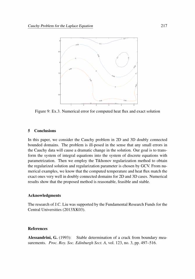
error of heat flux is given in Figure 9 for δ = 0.05 of relative noise. The root meansquare errors are ε(u) = 0.0163 and ε(u∗) = 0.0403 for the case of δ = 0.05. FromFigure 6 and Figure 8, it can be seen that numerical results match the exact onevery well for 3D case.


−0.1

−0.1

−0.1

−0.1

−0.05

−0.05

−0.05

−0.0

5

0

0

0

0

0.05

0.05

0.05 0.05

0.05

0.1 0.11 2 3 4 5 6

0.5

1

1.5

2

2.5

3

Figure 9: Ex.3. Numerical error for computed heat flux and exact solution

5 Conclusions

In this paper, we consider the Cauchy problem in 2D and 3D doubly connectedbounded domains. The problem is ill-posed in the sense that any small errors inthe Cauchy data will cause a dramatic change in the solution. Our goal is to trans-form the system of integral equations into the system of discrete equations withparametrization. Then we employ the Tikhonov regularization method to obtainthe regularized solution and regularization parameter is chosen by GCV. From nu-merical examples, we know that the computed temperature and heat flux match theexact ones very well in doubly connected domains for 2D and 3D cases. Numericalresults show that the proposed method is reasonable, feasible and stable.

Acknowledgments

The research of J.C. Liu was supported by the Fundamental Research Funds for theCentral Universities (2013XK03).

References

Alessandrini, G. (1993): Stable determination of a crack from boundary mea-surements. Proc. Roy. Soc. Edinburgh Sect. A, vol. 123, no. 3, pp. 497–516.


Ang, D. D.; Nghia, N. H.; Tam, N. C. (1998): Regularized solutions of a Cauchyproblem for the Laplace equation in an irregular layer: a three-dimensional model.Acta Math. Vietnam., vol. 23, no. 1, pp. 65–74.

Beale, J. T. (2004): A grid-based boundary integral method for elliptic problemsin three dimensions. SIAM J. Numer. Anal., vol. 42, no. 2, pp. 599–620.

Belgacem, F. B. (2007): Why is the Cauchy problem severely ill-posed? InverseProbl., vol. 23, pp. 823–36.

Belgacem, F. B.; Du, D. T.; Jelassi, F. (2011): Extended-domain-Lavrentiev’sregularization for the Cauchy problem. Inverse Probl., vol. 27, no. 4, pp. 045005.

Belgacem, F. B.; Fekih, H. E. (2005): On Cauchy’s problem: I. A variationalSteklov-Poincaré theory. Inverse Probl., vol. 21, no. 6, pp. 1915–36.

Berntsson, F.; Eldén, L. (2001): Numerical solution of a Cauchy problem for theLaplace equation. Inverse Probl., vol. 17, no. 4, pp. 839–853.

Calderon, A. P. (1958): Uniqueness in the Cauchy problem for partial differentialequations. American Journal of Mathematics, vol. 80, no. 1, pp. 16–36.

Chan, H. F.; Fan, C. M.; Yeih, W. (2011): Solution of inverse boundary opti-mization problem by Trefftz method and exponentially convergent scalar homotopyalgorithm. Computer Materials and Continua, vol. 24, no. 2, pp. 125.

Chapko, R.; Johansson, B. T. (2008): An alternating boundary integral basedmethod for a Cauchy problem for the Laplace equation in semi-infinite regions.Inverse Probl. Imaging, vol. 2, no. 3, pp. 317–333.

Chapko, R.; Johansson, B. T. (2008): An alternating potential-based approachto the Cauchy problem for the Laplace equation in a planar domain with a cut.Comput. Methods Appl. Math., vol. 8, no. 4, pp. 315–335.

Chapko, R.; Johansson, B. T. (2009): An alternating boundary integral basedmethod for a Cauchy problem for the Laplace equation in a quadrant. InverseProbl. Sci. Eng., vol. 17, no. 7, pp. 871–883.

Cheng, J.; Hon, Y.; Wei, T.; Yamamoto, M. (2001): Numerical computation ofa Cauchy problem for Laplace’s equation. ZAMM Z. Angew. Math. Mech, vol. 81,no. 10, pp. 665–674.

Cheng, J.; Prößdorf, S.; Yamamoto, M. (1998): Local estimation for an integralequation of first kind with analytic kernel. J. Inverse Ill-Posed Probl., vol. 6, no.2, pp. 115–126.

Chi, C. C.; Yeih, W.; Liu, C. S. (2009): A novel method for solving the cauchyproblem of laplace equation using the fictitious time integration method. ComputerModeling in Engineering and Sciences (CMES), vol. 47, no. 2, pp. 167.


Colli-Franzone, P.; Guerri, L.; Tentoni, S.; Viganotti, C.; Baruffi, S.; Spag-giari, S.; Taccardi, B. (1985): A mathematical procedure for solving the inversepotential problem of electrocardiography. analysis of the time-space accuracy fromin vitro experimental data. Mathematical Biosciences, vol. 77, no. 1-2, pp. 353 –396.

Dong, L.; Atluri, S. N. (2012): A Simple Multi-Source-Point Trefftz Method forSolving Direct/Inverse SHM Problems of Plane Elasticity in Arbitrary Multiply-Connected Domains. Computer Modeling in Engineering and Sciences (CMES),vol. 85, no. 1, pp. 1–43.

Gene, H. G.; Heath, M. T.; Wahba, G. (1979): Generalized Cross-Validationas a Method for Choosing a Good Ridge Parameter. Technometrics, vol. 21, pp.215–223.

Háo, D. N.; Lesnic, D. (2000): The Cauchy problem for Laplace’s equation viathe conjugate gradient method. IMA J. Appl. Math., vol. 65, no. 2, pp. 199–217.

Ivanyshyn, O.; Kress, R. (2006): Nonlinear integral equations for solving inverseboundary value problems for inclusions and cracks. J. Integral Equations Appl, vol.18, no. 1, pp. 13–38.

John, F. (1982): Partial Differential Equations. Applied Mathematical Sciences.Springer-Verlag, New York, fourth edition.

Klibanov, M. V.; Santosa, F. (1991): A computational quasi-reversibility methodfor Cauchy problems for Laplace’s equation. SIAM J Appl Math, vol. 51, no. 6,pp. 1653–1675.

Kress, R. (1999): Linear integral equations, volume 82 of Applied MathematicalSciences. Springer-Verlag, New York, second edition.

Lavrentev, M. M.; Romanov, V. G.; Shishatskii, S. P. (1986): Ill-posed prob-lems of mathematical physics and analysis, volume 64 of Translations of Mathe-matical Monographs. American Mathematical Society, Providence, RI. Translatedfrom the Russian by J. R. Schulenberger, Translation edited by Lev J. Leifman.

Liu, C. S. (2008): A highly accurate mctm for inverse cauchy problems of laplaceequation in arbitrary plane domains. Computer Modeling in Engineering and Sci-ences (CMES), vol. 35, no. 2, pp. 91–112.

Marin, L. (2009): An iterative mfs algorithm for the cauchy problem associ-ated with the laplace equation. Computer Modeling in Engineering and Sciences(CMES), vol. 48, no. 2, pp. 121.

Vani, C.; Avudainayagam, A. (2002): Regularized solution of the Cauchy prob-lem for the Laplace equation using meyer wavelets. Math. Comput. Model., vol.36, no. 9-10, pp. 1151 – 1159.

Cauchy Problem for the Laplace Equation in 2D and 3D ... Problem for the Laplace Equation in 2D and...

Documents

Transcript of Cauchy Problem for the Laplace Equation in 2D and 3D ... Problem for the Laplace Equation in 2D and...