Categorization and Annotation of Audiovisual Content · Informação retirada da literatura mostra...
76
FACULDADE DE E NGENHARIA DA UNIVERSIDADE DO P ORTO Categorization and Annotation of Audiovisual Content Filipe Pereira Leite Gabriel Mestrado Integrado em Engenharia Eletrotécnica e de Computadores Supervisor: Maria Teresa Andrade February 24, 2014
Transcript of Categorization and Annotation of Audiovisual Content · Informação retirada da literatura mostra...

FACULDADE DE ENGENHARIA DA UNIVERSIDADE DO PORTO
Categorization and Annotation ofAudiovisual Content
Filipe Pereira Leite Gabriel
Mestrado Integrado em Engenharia Eletrotécnica e de Computadores
Supervisor: Maria Teresa Andrade
February 24, 2014

c© Filipe Gabriel, 2014

Resumo
Geralmente, a classificação de conteúdos audiovisuais é feita manualmente, levando a um grauelevado de subjectividade na avaliação, o que leva normalmente a resultados incorrectos e inconsistentes.Com o crescimento exponencial da informação disponível, a maior parte dela não é classificadae quando o é, fica aquém do desejado. Com o aumento de serviços ao utilizador e de umaconsequente exigência, melhorar a classificação e sugestão de conteúdos é da máxima importância.Um conteúdo audiovisual pode ser descrito como uma combinação das suas propriedades. Entãopara o classificar, será lógico recorrer a elas. Informação retirada da literatura mostra que têmhavido esforços que vão no encontro de procurar e desenvolver ferramentas e técnicas que permitamcriar um sistema de classificação baseado nas características intrínsecas do conteúdo, mas atéagora os resultados têm sido incompletos em alguns pontos.O objetivo desta dissertação passa por desenvolver técnicas que permitam extrair as característicasde conteúdos audiovisuais e classificá-lo através delas. Através da pesquisa efetuada, foramseleccionadas as características mais importantes a extrair e foi desenvolvido o sistema a implementarpara o tratamento dos dados. Será composto por uma base de dados, uma interface web e oterminal responsável pela extracção das características.Este documento apresenta as técnicas e tecnologias usadas, bem como os resultados obtidosatravés dos classificadores de machine learning disponíveis. Foi possível constatar que mesmocom uma amostra pequena de conteúdos e um tempo de análise reduzido, é possível classificar esugerir conteúdos audiovisuais baseado nas suas características intrínsecas, com um considerávelgrau de eficácia.
i

ii

Abstract
Generally, audiovisual content classification is based on manual observation and is highly subjective,leading to flawed and inconsistent results. With the exponential growth of information available,most of it isn’t classified, and when it is, the accuracy is below par. Improving the classification andsuggestion of data is of the most importance with the increase of demand and services available.An audiovisual content can be described as a combination of its features. To classify the content,it is logical to resort to them. Retrieved information from the literature show that there have beenefforts to develop a classification system based on audiovisual features, but so far the results havebeen incomplete on some areas.This dissertation’s goal was to develop tools and techniques to extract and classify audiovisualcontent according to their intrinsic features. Based on the research conducted, the main features toextract were found and a system to treat the data was designed, which includes an user interface,a database and a terminal responsible for the analysis and extraction of the features.This document presents the techniques and technologies used and the results obtained usingmachine learning classifiers. They revealed that even with a small sample size and a limitedcontent analysis time, it is possible, and with some degree of efficiency, classify and suggestaudiovisual content based on its features.
iii

iv

Acknowledgements
First and foremost, I would like to thank my parents for giving me the chance to come this far inmy academic life.Thanks to all my friends that helped me in this dissertation and through all these years.Thanks to all the teachers that inspired me, and specially my supervisor, Maria Teresa Andrade,for her guidance and advices throughout the development of this dissertation.
Filipe Gabriel
v

vi

“I’ve failed over and over and over again in my life and that is why I succeed. ”
Michael Jordan
vii

viii
Contents
1 Introduction 11.1 Motivation . . . . . . . . . . . . . . . . . . . . . . . . . . . . . . . . . . . . . . 11.2 Scope . . . . . . . . . . . . . . . . . . . . . . . . . . . . . . . . . . . . . . . . 11.3 Objectives . . . . . . . . . . . . . . . . . . . . . . . . . . . . . . . . . . . . . . 21.4 Structure . . . . . . . . . . . . . . . . . . . . . . . . . . . . . . . . . . . . . . . 2
2 State of the Art 32.1 A/V features . . . . . . . . . . . . . . . . . . . . . . . . . . . . . . . . . . . . . 3
2.1.1 Relevant A/V features . . . . . . . . . . . . . . . . . . . . . . . . . . . 32.1.2 Features extraction . . . . . . . . . . . . . . . . . . . . . . . . . . . . . 32.1.3 Scene boundaries detection . . . . . . . . . . . . . . . . . . . . . . . . . 42.1.4 Image Segmentation . . . . . . . . . . . . . . . . . . . . . . . . . . . . 72.1.5 Edge detection . . . . . . . . . . . . . . . . . . . . . . . . . . . . . . . 10
2.2 Facial Recognition . . . . . . . . . . . . . . . . . . . . . . . . . . . . . . . . . 112.2.1 Facial Detection . . . . . . . . . . . . . . . . . . . . . . . . . . . . . . 112.2.2 Face Recognition . . . . . . . . . . . . . . . . . . . . . . . . . . . . . . 12
2.3 Machine Learning . . . . . . . . . . . . . . . . . . . . . . . . . . . . . . . . . . 132.3.1 Classifiers . . . . . . . . . . . . . . . . . . . . . . . . . . . . . . . . . . 132.3.2 ARFF files . . . . . . . . . . . . . . . . . . . . . . . . . . . . . . . . . 15
2.4 Technologies and Methodologies . . . . . . . . . . . . . . . . . . . . . . . . . . 162.4.1 Development environments . . . . . . . . . . . . . . . . . . . . . . . . 162.4.2 Global development . . . . . . . . . . . . . . . . . . . . . . . . . . . . 17
2.5 Conclusions . . . . . . . . . . . . . . . . . . . . . . . . . . . . . . . . . . . . . 18
3 Specification of the adopted solution 213.1 Techniques and Technologies . . . . . . . . . . . . . . . . . . . . . . . . . . . . 213.2 System . . . . . . . . . . . . . . . . . . . . . . . . . . . . . . . . . . . . . . . . 22
3.2.1 Architecture . . . . . . . . . . . . . . . . . . . . . . . . . . . . . . . . . 223.2.2 Functionalities . . . . . . . . . . . . . . . . . . . . . . . . . . . . . . . 22
4 Development 254.1 Overview . . . . . . . . . . . . . . . . . . . . . . . . . . . . . . . . . . . . . . 25
4.1.1 Database . . . . . . . . . . . . . . . . . . . . . . . . . . . . . . . . . . 254.1.2 Matlab . . . . . . . . . . . . . . . . . . . . . . . . . . . . . . . . . . . 264.1.3 Interface . . . . . . . . . . . . . . . . . . . . . . . . . . . . . . . . . . 30
4.2 Results . . . . . . . . . . . . . . . . . . . . . . . . . . . . . . . . . . . . . . . . 324.2.1 Shot boundaries detection algorithm . . . . . . . . . . . . . . . . . . . . 324.2.2 Face Recognition . . . . . . . . . . . . . . . . . . . . . . . . . . . . . . 33
ix

x CONTENTS
4.2.3 Low level A/V features . . . . . . . . . . . . . . . . . . . . . . . . . . . 334.2.4 A/V content classification . . . . . . . . . . . . . . . . . . . . . . . . . 34
4.3 Conclusions . . . . . . . . . . . . . . . . . . . . . . . . . . . . . . . . . . . . . 36
5 Conclusions and future work 395.1 Conclusions . . . . . . . . . . . . . . . . . . . . . . . . . . . . . . . . . . . . . 395.2 Future work . . . . . . . . . . . . . . . . . . . . . . . . . . . . . . . . . . . . . 39
A Decision trees 41A.1 Decision Trees - A/V content clasification . . . . . . . . . . . . . . . . . . . . . 41
A.1.1 5 minutes . . . . . . . . . . . . . . . . . . . . . . . . . . . . . . . . . . 41A.1.2 10 minutes . . . . . . . . . . . . . . . . . . . . . . . . . . . . . . . . . 45
A.2 Decision Trees - shot boundaries . . . . . . . . . . . . . . . . . . . . . . . . . . 51

List of Figures
2.1 Grayscale histogram example . . . . . . . . . . . . . . . . . . . . . . . . . . . . 52.2 Transition types with ECR . . . . . . . . . . . . . . . . . . . . . . . . . . . . . 62.3 Threshold on a bimodal image histogram . . . . . . . . . . . . . . . . . . . . . 72.4 T value . . . . . . . . . . . . . . . . . . . . . . . . . . . . . . . . . . . . . . . 72.5 Multilevel threshold . . . . . . . . . . . . . . . . . . . . . . . . . . . . . . . . 82.6 Example of region growing . . . . . . . . . . . . . . . . . . . . . . . . . . . . . 92.7 Example of split and merge . . . . . . . . . . . . . . . . . . . . . . . . . . . . . 92.8 Face outline result . . . . . . . . . . . . . . . . . . . . . . . . . . . . . . . . . . 112.9 Eyes Location . . . . . . . . . . . . . . . . . . . . . . . . . . . . . . . . . . . . 122.10 Multiple hyperplanes . . . . . . . . . . . . . . . . . . . . . . . . . . . . . . . . 152.11 Optimal hyperplane, maximum margin and support vectors . . . . . . . . . . . . 152.12 ARFF file example . . . . . . . . . . . . . . . . . . . . . . . . . . . . . . . . . 16
3.1 System’s architecture . . . . . . . . . . . . . . . . . . . . . . . . . . . . . . . . 22
4.1 Entity-Association model . . . . . . . . . . . . . . . . . . . . . . . . . . . . . . 254.2 Fades detection criteria . . . . . . . . . . . . . . . . . . . . . . . . . . . . . . . 264.3 Hard cuts detection criteria . . . . . . . . . . . . . . . . . . . . . . . . . . . . . 274.4 Sobel gradient output . . . . . . . . . . . . . . . . . . . . . . . . . . . . . . . . 284.5 Example of face detection . . . . . . . . . . . . . . . . . . . . . . . . . . . . . 284.6 Training set of images . . . . . . . . . . . . . . . . . . . . . . . . . . . . . . . . 294.7 Average face of the training set of images . . . . . . . . . . . . . . . . . . . . . 294.8 Example of an image’s features . . . . . . . . . . . . . . . . . . . . . . . . . . . 294.9 UI main page - analyzing content . . . . . . . . . . . . . . . . . . . . . . . . . . 304.10 UI main page - results ready . . . . . . . . . . . . . . . . . . . . . . . . . . . . 314.11 List of suggestions after 5 minutes. Genre suggested is action, which is incorrect 314.12 List of suggestions after 10 minutes. Genre suggested is horror, which is correct . 324.13 J48 5 minutes 28 videos decision tree . . . . . . . . . . . . . . . . . . . . . . . 354.14 J48 10 minutes 28 videos decision tree . . . . . . . . . . . . . . . . . . . . . . . 36
A.1 J48 5 minutes 12 videos decision tree . . . . . . . . . . . . . . . . . . . . . . . 42A.2 RandomTree 5 minutes 12 videos decision tree . . . . . . . . . . . . . . . . . . 42A.3 REPTree 5 minutes 12 videos decision tree . . . . . . . . . . . . . . . . . . . . 42A.4 J48 5 minutes 20 videos decision tree . . . . . . . . . . . . . . . . . . . . . . . 43A.5 RandomTree 5 minutes 20 videos decision tree . . . . . . . . . . . . . . . . . . 43A.6 REPTree 5 minutes 20 videos decision tree . . . . . . . . . . . . . . . . . . . . 43A.7 J48 5 minutes 28 videos decision tree . . . . . . . . . . . . . . . . . . . . . . . 44A.8 RandomTree 5 minutes 28 videos decision tree . . . . . . . . . . . . . . . . . . 44A.9 REPTree 5 minutes 28 videos decision tree . . . . . . . . . . . . . . . . . . . . 44
xi

xii LIST OF FIGURES
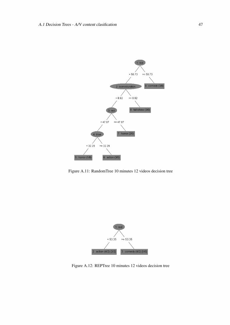
A.10 J48 10 minutes 12 videos decision tree . . . . . . . . . . . . . . . . . . . . . . . 46A.11 RandomTree 10 minutes 12 videos decision tree . . . . . . . . . . . . . . . . . . 47A.12 REPTree 10 minutes 12 videos decision tree . . . . . . . . . . . . . . . . . . . . 47A.13 J48 10 minutes 20 videos decision tree . . . . . . . . . . . . . . . . . . . . . . . 48A.14 RandomTree 10 minutes 20 videos decision tree . . . . . . . . . . . . . . . . . . 48A.15 REPTree 10 minutes 20 videos decision tree . . . . . . . . . . . . . . . . . . . . 49A.16 J48 10 minutes 28 videos decision tree . . . . . . . . . . . . . . . . . . . . . . . 49A.17 RandomTree 10 minutes 28 videos decision tree . . . . . . . . . . . . . . . . . . 49A.18 REPTree 10 minutes 28 videos decision tree . . . . . . . . . . . . . . . . . . . . 50A.19 J48 Clip 1 decision tree . . . . . . . . . . . . . . . . . . . . . . . . . . . . . . . 52A.20 RandomTree Clip 1 decision tree . . . . . . . . . . . . . . . . . . . . . . . . . . 52A.21 REPTree Clip 1 decision tree . . . . . . . . . . . . . . . . . . . . . . . . . . . . 53A.22 J48 Clip 2 decision tree . . . . . . . . . . . . . . . . . . . . . . . . . . . . . . . 53A.23 RandomTree Clip 2 decision tree . . . . . . . . . . . . . . . . . . . . . . . . . . 53A.24 REPTree Clip 2 decision tree . . . . . . . . . . . . . . . . . . . . . . . . . . . . 54A.25 J48 Clip 3 decision tree . . . . . . . . . . . . . . . . . . . . . . . . . . . . . . . 54A.26 RandomTree Clip 3 decision tree . . . . . . . . . . . . . . . . . . . . . . . . . . 55A.27 REPTree Clip 3 decision tree . . . . . . . . . . . . . . . . . . . . . . . . . . . . 56
List of Tables
4.1 Shot boundaries detection with 10% as criteria . . . . . . . . . . . . . . . . . . . 334.2 Action: features values . . . . . . . . . . . . . . . . . . . . . . . . . . . . . . . 334.3 Horror: features values . . . . . . . . . . . . . . . . . . . . . . . . . . . . . . . 344.4 Comedy: features values . . . . . . . . . . . . . . . . . . . . . . . . . . . . . . 344.5 Talkshow: features values . . . . . . . . . . . . . . . . . . . . . . . . . . . . . . 34
A.1 Correctly classified instances - 5 minutes 12 videos . . . . . . . . . . . . . . . . 41A.2 Correctly classified instances - 5 minutes 20 videos . . . . . . . . . . . . . . . . 41A.3 Correctly classified instances - 5 minutes 28 videos . . . . . . . . . . . . . . . . 41A.4 Correctly classified instances - 10 minutes 12 videos . . . . . . . . . . . . . . . 46A.5 Correctly classified instances - 10 minutes 20 videos . . . . . . . . . . . . . . . 46A.6 Correctly classified instances - 10 minutes 28 videos . . . . . . . . . . . . . . . 46A.7 DecisionStump output clip 1 . . . . . . . . . . . . . . . . . . . . . . . . . . . . 52A.8 DecisionStump output clip 2 . . . . . . . . . . . . . . . . . . . . . . . . . . . . 52A.9 DecisionStump output clip 3 . . . . . . . . . . . . . . . . . . . . . . . . . . . . 52
xiii

xiv LIST OF TABLES

Symbols and Abbreviations
AI Artificial IntelligenceARFF Attribute Relationship File FormatA/V AudiovisualCSS Cascading Style SheetHTML Hypertext Markup LanguageINESC Instituto de Engenharia de Sistemas e ComputadoresIPTV Internet Protocol TelevisionJS Java ScriptLoG Laplacian of GaussianMATLAB Matrix LaboratorySFX Special EffectsSVM Supporting Vector MachinesTMU Telecommunications Multimedia UnitUI User InterfaceWEKA Waikato Environment for Knowledge Analysis
xv


Chapter 1
Introduction
This chapter describes the structure of the document and presents the dissertation’s scope, its
motivations and the main objectives.
1.1 Motivation
Nowadays, searching for the desired or useful information can be extremely hard as the amount of
information available is enormous and continuously grows every year. Currently available search
mechanisms often lead to incorrect results, mostly due to the unavailability of content descriptions
or to the availability of incorrect or disparate tags.
The most usual searching engines are based on keywords attached to the available resources.
However, the process of creating these tags is usually manual which leads to subjective analysis.
Therefore there is the need to use other alternatives for the generation and insertion of descriptive
tags, preferably based on intrinsic content information, removing all the subjectivity and human
interference in the process.
There has been an effort to develop a base of knowledge containing the most important features of
audiovisual (A/V) content, but the results so far are somewhat incomplete in some areas.
The possibility to describe, categorize and suggest A/V content in an automated or assisted way,
bringing more accuracy to the process proves to be challenging, innovative and with the available
A/V content distributors on the market, necessary.
1.2 Scope
This dissertation was proposed by INESC Porto TMU and its ambitions are to incorporate new
techniques in analysis and annotation of A/V content, which would increase the capabilities of
existing distribution services such as IPTV services, social networks and local applications that
store and manage A/V content.
1
2 Introduction
1.3 Objectives
As referred previously, the main objective overall for this dissertation is to develop tools to classify
A/V content and build an initial knowledge base on categories of A/V content. These will then be
used to represent and categorize A/V content in different application scenarios. The main goal is
to identify and suggest similar content based on these categorizations within different contexts.
As the ambition is to increase the capabilities of existing services, there are three main areas of
interest that will be taken into account:
• IPTV Services: Ability to analyze and categorize shows, series or movies that are being
watched by the user at that moment and then give suggestions based on those results.
• Social Networks: The objective is to analyze and categorize the published content by a user,
search similar content and then give the suggestion based on those results.
• Storage and Management of A/V content applications: In this case, the user must categorize
the content. In order to reduce the subjectivity of the process, there should be an automatic
analysis and categorization of the content. This automated process can be used to enhance
or refine existing descriptions that have been previously inserted by a human. Conversely,
once generated, these keywords may assist a human when inserting additional descriptive
data. This can be useful in professional environments such as A/V post-production, helping
to create accurately annotated archives, which are easily searchable. . . .
1.4 Structure
This document is structured in five different chapters: introduction, state of the art, specification
of the adopted solution, development and conclusions and future work.
The first chapter presents the dissertation’s scope, its motivations and the main objectives.
The state of the art chapter reviews the most relevant A/V features, what they represent and the
techniques that allow their extraction and research about face recognition and machine learning.
The third chapter, specification of the adopted solution, presents the designed solutions, techniques
and technologies to the diverse areas of the dissertation as well as the system architecture and
functionalities.
The development chapter focuses on the work developed along the course of the dissertation and
the results obtained.
Finally, the fifth and final chapter presents the dissertation’s conclusions and some notes to future
work.

Chapter 2
State of the Art
This chapter describes the techniques to extract the relevant features to properly analyze the A/V
content.
First, it presents a commonly accepted list of the relevant features of the A/V content that can help
in obtaining a high-level characterization of the content. They can be separated in two categories:
low level or high level features. Then it is briefly explained how those features can be extracted
and what they represent.
2.1 A/V features
2.1.1 Relevant A/V features
To properly classify the A/V content, there is a set of low-level features that can be useful to
identify the type of content in some way: [1,2]
• Color
• Brightness
• Motion
• Rhythm
There are also high level features that may provide help in the categorization of the content:
• Scene Duration
• Facial Recognition
2.1.2 Features extraction
In this dissertation, the features will be extracted from images retrieved from video files. This
means that it must be taken in consideration what kind of video is being analyzed to make the
correct suggestions of similar content.
3
4 State of the Art
In order to extract the features from the A/V content, there are techniques that are useful and
are described below:
• Color
Each frame from a movie contains information about color. Each pixel of the frame is represented
by a combination of the 3 primary colors: red, green and blue. It can be viewed as a 3 dimensional
parallel plane. On that consideration, it is easy to get information about any primary color on each
frame by isolating each plane.
• Brightness
Brightness can be obtained from each frame in two different ways: change the video color space
from RGB to YUV and extract the Y plane, which represents the luminance component, or stay
on the RGB color space and compute the Y component through the RGB components.
• Motion
Intuitively, motion through a video can be perceived as the amount of movement objects undergo.
Therefore, to get the amout of motion, it is necessary to isolate objects in every frame and calculate
how much they moved in consecutive or a block of frames.
• Rhythm
Intuitively, the perception of rhythm is related to how fast the pace of the content is. If two
contents, A and B, with the same time duration contain different number of scenes, we can
conclude that A has a higher rhythm than B or vice-versa. On that note, detection of scene
boundaries is fundamental.
• Scene Duration
With the scene boundaries frames detected, with a conversion from frames to a time variable using
the framerate, it is possible to calculate scene durations.
To extract the features from the A/V content, there are techniques that are useful and are described
below.
2.1.3 Scene boundaries detection
Scene Boundaries Detection is a key part in the context of this dissertation as the extraction of
some of the features only makes sense in this context. The boundaries of a scene can be detected
in their transition, which can be indicated by hard cuts, fades and dissolves.
Hard cuts can be defined as instantaneous transitions from one scene to another. Fades are defined
as gradual transitions between a scene and a constant image, normally solid black or white. If the
transition is from the image to the scene, it is considered as a fade-in and the opposite is considered

2.1 A/V features 5
as a fade-out. Dissolves are gradual transitions between scenes, where the first scene fades out and
the next scene fades in at the same time and with constant fade rate. [3][4]
Algorithms to detect fades, dissolves and hard cuts are discussed by Rainer Lienhart on [5] and
the two most important that cover all the transition types in the literature are:
• Color Histogram Differences
Histograms are a graphical representation of the distribution of data. In an image, histograms
represent the distribution of the image’s pixel intensities. On the figure 2.1 it is represented an
example of a grayscale histogram. The x axis represent all the 256 possible intensities and the y
axis represent their occurrence.
The basic concept is that the color content of the frames does not change within the scene but
across them. This way, the difference between color histograms from consecutive frames can
detect if a transition occurs. Due to the nature of this algorithm, it gives good results on hard cuts
transitions.
Figure 2.1: Grayscale histogram example
• Edge Change Ratio
This algorithm relies on the idea that edges of the objects that belong to a scene would definitely
change across a boundary. To identify the edges on the image, it is used the Canny Edge detector.
This detection algorithm is divided in 3 steps: Smoothing, Enhancement and Detection.
On the smoothing phase, the image is Gaussian filtered followed by gradient and orientation
computation.
The enhancement phase requires a non-maximum suppression step, which thins the ridges of the
gradient magnitude by suppressing all values along the line of the gradient that are not peaks
values of the ridge.
The detection phase is characterized by the use of a double threshold operator that reduces the
number of false edge segments.
Another famous edge detection algorithm is the Marr and Hildreth Edge Detector that consists in
a combination from a Gaussian filter and a Laplacian edge detector, the LoG. The fundamental
characteristics of this detector are:

6 State of the Art
• Smoothing phase is Gaussian filtering, to remove high frequency noise;
• Enhancement step is the Laplacian;
• The detection criteria is the presence of the zero crossing in the 2nd derivative (Laplacian),
combined with a corresponding large peak in the 1st derivative (Gaussian). Here, only
the zero crossings whose corresponding 1st derivative is above a specified threshold are
considered;
• The edge location can be estimated using sub-pixel resolution by interpolation.
The output of the algorithm, Edge Change Ratio (ECR), across the analyzed frames, defines
the type of transitions. Hard cuts are recognized as isolated peaks; during fades the number of
incoming/outgoing edges predominates; during dissolves, the outgoing edges of the first scene
protrude before the incoming edges of the second scene start to dominate the second half of a
dissolve. The representation is shown in the figure 2.2.
Figure 2.2: Transition types with ECR
The conclusions on the performance of the scene boundaries detection algorithms are:
• The color histogram differences algorithm provides better results than the edge change ratio
in hard cuts transitions.
• The edge change ratio algorithm doesn’t provide good results in dissolves and fades.
• There is the need to search for another alternative to detect fades and dissolves. Fades can be
detected by the Standard Deviation of Pixel Intensities: it consists in finding monochromatic
frame sequences which is identified by a sequence of frames whose standard deviation of
pixel intensities is below a certain value. A Contrast Change algorithm was designed to
detect dissolves, but with videos with few dissolve transitions, the results were extremely
unsatisfactory, as the false hits number was a lot bigger than the number of actual dissolve
transitions in the tested videos.
2.1 A/V features 7
2.1.4 Image Segmentation
Image segmentation [6] is the process of portioning the image into multiple segments.
Segmenting allows a better representation of a certain area of the image which enables a more
precise analysis and specificities of the regions, providing a greater level of global information
about the image.
Image segmentation methods can be categorized in two different domains: feature and image.
The idea behind feature domain is to measure several features and organize them into a feature
vector and use clustering methods to segment the data. Depending on the problem there can be
used many features such as intensity, color, texture and position. Each feature component may
characterize a single pixel (as the intensity) or a region (as the area). Some of the most important
feature domain methods are:
• Otsu Method
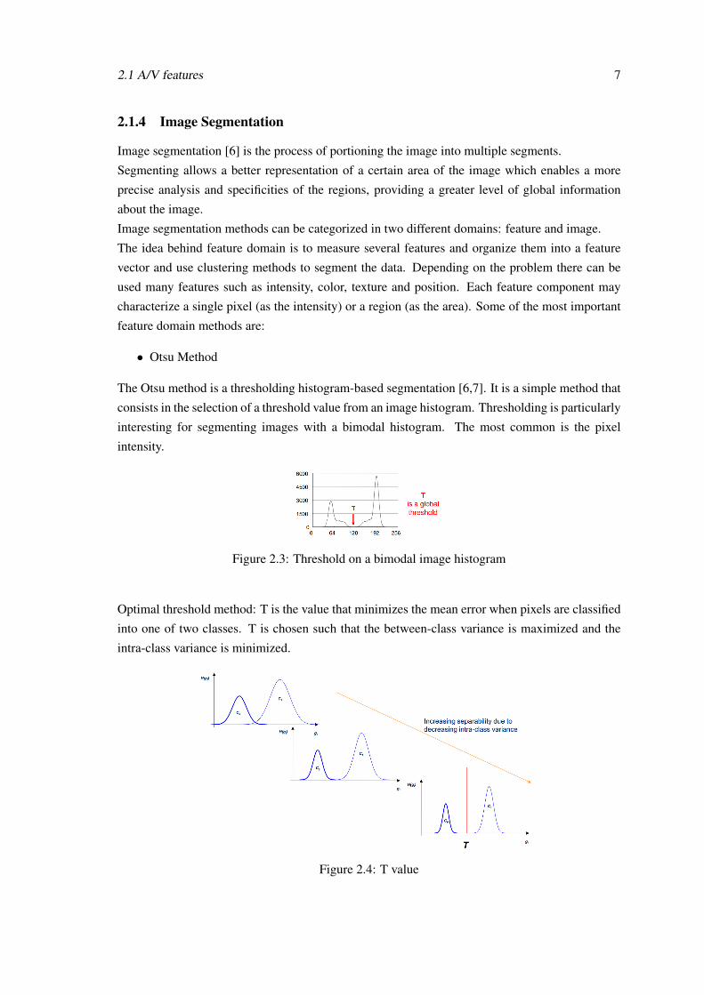
The Otsu method is a thresholding histogram-based segmentation [6,7]. It is a simple method that
consists in the selection of a threshold value from an image histogram. Thresholding is particularly
interesting for segmenting images with a bimodal histogram. The most common is the pixel
intensity.
Figure 2.3: Threshold on a bimodal image histogram
Optimal threshold method: T is the value that minimizes the mean error when pixels are classified
into one of two classes. T is chosen such that the between-class variance is maximized and the
intra-class variance is minimized.
Figure 2.4: T value

8 State of the Art
The thresholding concept can be used when the image has more than two regions (more than two
modes in the histogram).
Figure 2.5: Multilevel threshold
• K-means
K-means is a clustering method which objective is to partition data points in k clusters [6]. The
algorithm is composed by 4 steps:
• Choose k data points to act as cluster centers.
• Assign each data point to the cluster whose center is closest.
• Replace the cluster centers with the actual mean.
• Repeat steps 2 and 3 until convergence is reached.
Some of the most famous image domain segmentation methods are:
• Region growing
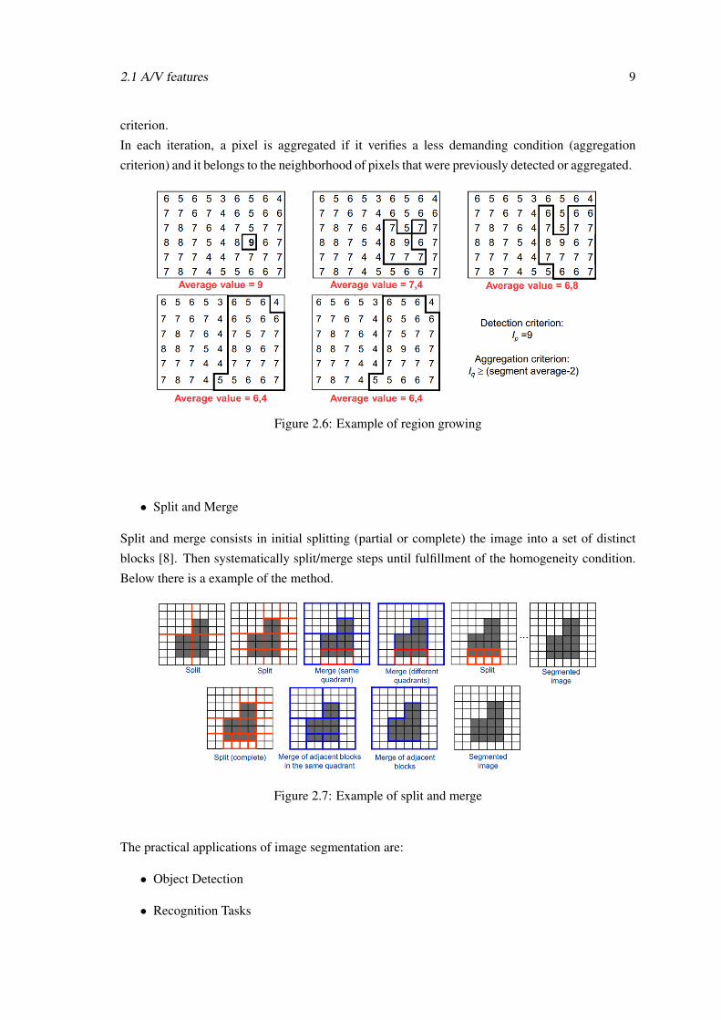
Region growing [8] is a very flexible iterative approach for the sequential extraction of objects
starting from an initial set of points (seeds). Seeds are obtained using a highly selective detection
2.1 A/V features 9
criterion.
In each iteration, a pixel is aggregated if it verifies a less demanding condition (aggregation
criterion) and it belongs to the neighborhood of pixels that were previously detected or aggregated.
Figure 2.6: Example of region growing
• Split and Merge
Split and merge consists in initial splitting (partial or complete) the image into a set of distinct
blocks [8]. Then systematically split/merge steps until fulfillment of the homogeneity condition.
Below there is a example of the method.
Figure 2.7: Example of split and merge
The practical applications of image segmentation are:
• Object Detection
• Recognition Tasks

10 State of the Art
Object detection reveals to be important in the calculation of the Motion feature, as discussed in
[2]. The image segmentation algorithm identifies objects that are consistent in color and texture.
Then, it must identify which of those objects undergo the highest amount of motion, using for
that purpose MPEG motion vectors. After that detection, it is measured the distance those objects
travel along the scene based on the movement of their centroids. Then, depending on the distance
value the scene can be classified as either action or non-action.
Image segmentation proves to be a good technique to extract features from A/V content in the
form of either feature/image domain methods or morphological operations.
2.1.5 Edge detection
Edge detection [9] is the essential operation of detecting intensity variations.
1st and 2nd derivative operators give the information of this intensity changes.
∇ f = [∂ f∂x
,∂ f∂y
]′ (2.1)
= [Ix, Iy]′ (2.2)
The gradient of the image intensity is given by equation 2.1 and its magnitude by equation 2.3.
G =√
I2x + I2
y (2.3)
The most usual gradient operators are:
• Roberts
Ix ≈
1 0
0 −1
; Iy ≈
0 −1
1 0
(2.4)
• Prewitt
Ix ≈
−1 0 1
−2 0 2
−1 0 1
; Iy ≈
1 2 1
0 0 0
−1 −2 −1
(2.5)
• Sobel
Ix ≈
−1 0 1
−1 0 1
−1 0 1
; Iy ≈
1 1 1
0 0 0
−1 −1 −1
(2.6)

2.2 Facial Recognition 11
2.2 Facial Recognition
2.2.1 Facial Detection
Facial recognition, in the scope of this dissertation, should be a good feature to focus on as it is
possible to connect certain individuals to a certain genre, adding value to the classification method,
as well as the suggestions list. Instinctively, it is possible to think of a certain genre when a known
face is recognized in a movie, obtaining in a matter of seconds the categorization, based on the
recognition of the individual (for example, movies starring John Wayne or Jim Carrey are easily
related to specific genres).
Several approaches are made in the literature for face detection, especially aiming to the lips [10]
and eyes detection.
Face detection and recognition using Matlab is addressed in [11] and the method is described
below.
For the face detection phase, the focus is to detect the eyes. For that purpose, the authors’ method
has the following steps:
• Light Compensation on the image, to improve the algorithm performance.
• Transformation to the YCbCr space for easier skin detection. Skin regions and eyes can
be extracted using information in the chrominance components. High levels of Cb values
and low levels of Cr values are especially found in eye regions. Converting the image to
YCbCr color space ensures that the algorithm still maintains robust for both dark and light
skin-colors. The reason for this is that the skin-tone color depends on the luminance. For
varying illumination, a better performance is obtained by using YCbCr compared with the
RGB color-space.
• As chrominance can be separated from luminance, to localize the outline of a face the
chrominance components are thresholded.
• Morphological operations are used to extract skin-regions and eliminate noise. The result is
a facemask which can be used to remove everything except skin-regions.
• Morphological operations and histogram equalization are used to obtain the location of the
eyes.
Figure 2.8: Face outline result
12 State of the Art
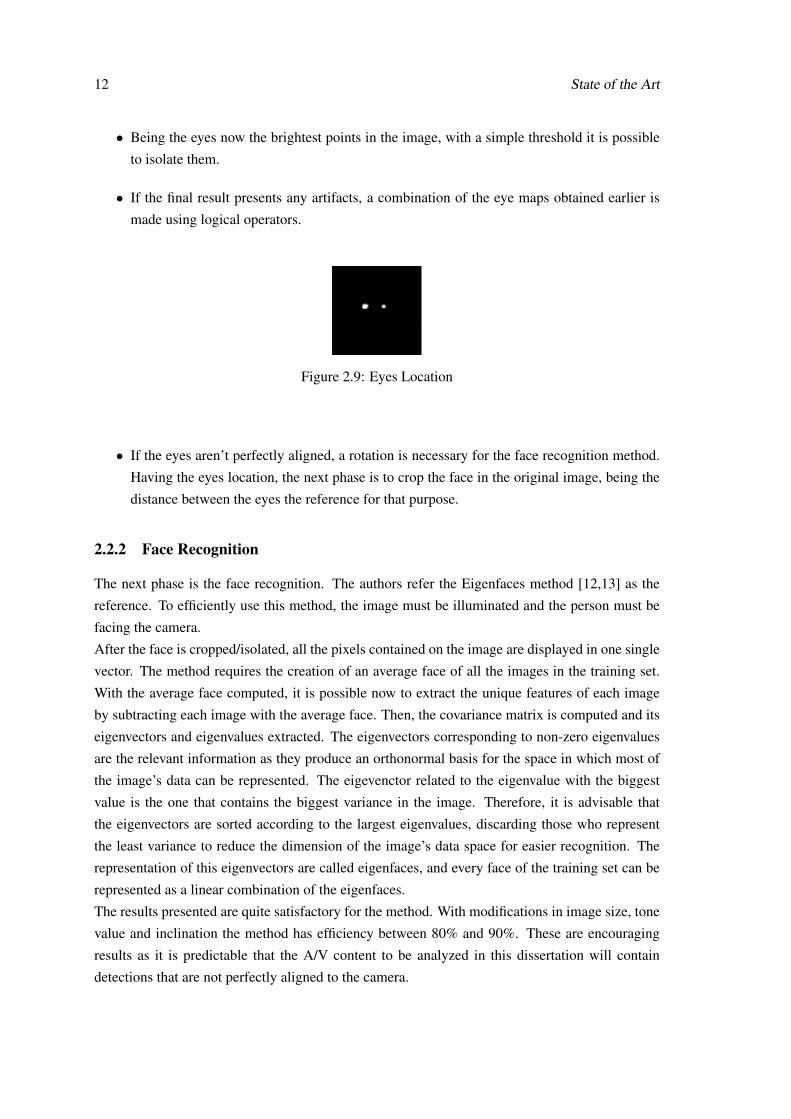
• Being the eyes now the brightest points in the image, with a simple threshold it is possible
to isolate them.
• If the final result presents any artifacts, a combination of the eye maps obtained earlier is
made using logical operators.
Figure 2.9: Eyes Location
• If the eyes aren’t perfectly aligned, a rotation is necessary for the face recognition method.
Having the eyes location, the next phase is to crop the face in the original image, being the
distance between the eyes the reference for that purpose.
2.2.2 Face Recognition
The next phase is the face recognition. The authors refer the Eigenfaces method [12,13] as the
reference. To efficiently use this method, the image must be illuminated and the person must be
facing the camera.
After the face is cropped/isolated, all the pixels contained on the image are displayed in one single
vector. The method requires the creation of an average face of all the images in the training set.
With the average face computed, it is possible now to extract the unique features of each image
by subtracting each image with the average face. Then, the covariance matrix is computed and its
eigenvectors and eigenvalues extracted. The eigenvectors corresponding to non-zero eigenvalues
are the relevant information as they produce an orthonormal basis for the space in which most of
the image’s data can be represented. The eigevenctor related to the eigenvalue with the biggest
value is the one that contains the biggest variance in the image. Therefore, it is advisable that
the eigenvectors are sorted according to the largest eigenvalues, discarding those who represent
the least variance to reduce the dimension of the image’s data space for easier recognition. The
representation of this eigenvectors are called eigenfaces, and every face of the training set can be
represented as a linear combination of the eigenfaces.
The results presented are quite satisfactory for the method. With modifications in image size, tone
value and inclination the method has efficiency between 80% and 90%. These are encouraging
results as it is predictable that the A/V content to be analyzed in this dissertation will contain
detections that are not perfectly aligned to the camera.

2.3 Machine Learning 13
2.3 Machine Learning
Machine learning is an Artificial Intelligence (AI) discipline which goal is to give computers the
ability to learn from data, in order to improve its own performance. Machine learning searches
through data to find patterns not for human comprehension but to improve the program’s own
understanding.
As this dissertation focuses on data categorization, it is logical to research about machine learning
algorithms that relate to data classification.
2.3.1 Classifiers
Decision trees
A decision tree [14] is a predictive machine learning model that uses a tree-like graph that decides
the value of a dependent variable given the values of several independent input variables. The
internal nodes indicate the different attributes, the branches tell the possible values that the attributes
can have and the leafs or terminal nodes indicate the final value to the output dependent variable.
Some of the advantages of decision trees are:
• Easy to interpret;
• Easy to incorporate a range of numeric or categorical data layers and there is no need to
select unimodal training data;
• Allows a variety of input data: Nominal, Numeric and Textual;
• Robust to discrepancies in training data;
• Fast classification.
Some of the disadvantages of decision trees:
• Decision trees tend to overfit training data which can give poor results when applied to the
full data set;
• Not possible to predict beyond the minimum and maximum limits of the response variable
in the training data;
• Multiple output attributes are not allowed.

14 State of the Art
Decision trees algorithms available on the machine learning software WEKA
• J48
J48 is WEKA’s implementation of C4.5 algorithm, which generates the decision tree based on
the attribute values of the available training data. It identifies the attribute that discriminates the
various instances most clearly. This feature that is able to tell the most about the data instances is
said to have the highest information gain. Among the possible values of this feature, if there is any
value for which there is no ambiguity, it is assigned to the target value. This process is repeated
for other attributes that give the highest information gain until there are no attributes left or there
is no more unambiguous results from the data.
• REPTree
REPTree builds a decision tree using entropy as impurity measure and prunes it using reduced-error
pruning.
It only sorts values for numeric attributes once.
• RandomTree
Random decision tree algorithm constructs multiple decision trees randomly. It considers a set of
K randomly chosen attributes to split on at each node. Depending on the nature of the feature,
it can be chosen to be picked up again on the same decision path. Features with limited or fixed
number of possible values are not picked if they were already chosen on the path. Everytime the
feature is selected, the threshold associated is randomly chosen.
The tree stops its growth when a node becomes empty or the depth of tree exceeds some limits.
• DecisionStump
DesicionStump is a tree constituted by only one level, where the decision is based on a specific
attribute and value.
SVM
A Support Vector Machine (SVM) is a discriminative classifier formally defined by a separating
hyperplane. Given labeled training data, the algorithm outputs an optimal hyperplane which
categorizes new incoming data into one category or the other.
Picture 2.10 represents labeled training data. The line that separates both labeled data is not
unique.

2.3 Machine Learning 15
Figure 2.10: Multiple hyperplanes
The goal of SVM is to find the optimal hyperplane that ensures the best margin, when the new
incoming data is about to be classified. That is achieved by finding the line that crosses as far
as possible from all the points. The optimal separating hyperplane maximizes the margin of the
training data. The picture below represents the optimal hyperplane and the maximum margin for
the given distribution.
Figure 2.11: Optimal hyperplane, maximum margin and support vectors
2.3.2 ARFF files
ARRF is the text format file used by WEKA to store data in a database. The ARFF file contains
two sections: the header and the data section. The first line of the header tells us the relation
name. Then there is the list of the attributes (@attribute...). Each attribute is associated with a
unique name and a type. The latter describes the kind of data contained in the variable and what
values it can have. The variables types are: numeric, nominal, string and date.

16 State of the Art
Figure 2.12: ARFF file example
2.4 Technologies and Methodologies
2.4.1 Development environments
• WEKA
The WEKA machine learning workbench provides a general-purpose environment for automatic
classification, regression, clustering and feature selection—common data mining problems. It
contains an extensive collection of machine learning algorithms and data pre-processing methods
complemented by graphical UI for data exploration and the experimental comparison of different
machine learning techniques on the same problem. WEKA can process data given in the form of
a single relational table. [15]
• MATLAB
MATLAB is a high-level language and interactive environment for numerical computation, visualization
and programming.
MATLAB allows matrix manipulations, plotting of functions and data, implementation of algorithms,
creation of UI, and interfacing with programs written in other languages, including C, C++ and
Java.
On the context of this dissertation, MATLAB is essential as it provides toolboxes to deal with video
and image processing, matrix manipulations that are essential to image processing, extraction
of features in the form of histograms and the ability to use pre-existed algorithms for image
segmentation and edge detection for example.

2.4 Technologies and Methodologies 17
2.4.2 Global development
As the UI will be web-oriented, below are described the technologies that will help the development
of the designed system.
• SQL
SQL is a standard computer language for relational database management and data manipulation.
It is used to query, insert, update and modify data. As most relational databases support SQL, it is
a benefit for database administrators.
• PHP
PHP is a scripting language suited to server-side web development and used to create dynamic
and interactive web pages. It can be deployed on most web servers and used with most relational
database management systems.
• HTML
HTML is the major markup language used to display web pages that can be displayed in a web
browser. Web pages are composed of HTML, which is used to display text, images or other
resources through a web server. It is the easiest and most powerful way to develop a website (in
association with a style sheet).
The Current version and base for future drafts is the HTML5.
• CSS
CSS is a standard that describes the formatting of markup language pages. It enables the separation
of content and visual elements such as the layout, colors and fonts for better page control and
flexibility. Web browsers can refer to CSS to define the appearance and layout of text and other
material in a document written in HTML.
• JS
JS is a scripting language that can interact with HTML source, which enables the presentation of
dynamic content on websites and enhanced UI.
• Smarty
Smarty is a php web template system which main goal is to separate the presentation from the
business logic, as dealing with PHP statements and HTML code together can become hard to
manage. Smarty allows PHP programmers to define custom functions that can be accessed using
Smarty tags.

18 State of the Art
2.5 Conclusions
With the features and their extracting techniques reviewed, there are some conclusions to make
towards understanding how can those features help in the categorization of A/V content.
The list below represents the most important features to extract and their contribution:
Color
• Color histograms in scene boundaries detection;
• Image segmentation in object detection to calculate the motion feature;
• Valuable information for specific content characterization, such as sports and TV news
programs, which in most of the time, the color histogram would be very similar for a great
number of scenes;
• According to [1], color on its own is not a good feature to classify movies, as it isn’t
particular enough to the diverse genres.
Brightness
• Valuable information for specific content characterization, such as indoor/outdoor scenes;
• Valuable for facial detection and recognition purposes;
• According to [1], brightness on its own is not a good feature to classify movies, as it isn’t
particular enough to the diverse genres.
Motion
• Motion is a valuable asset in limiting the number of possible classifications.
Rhythm
• Rhythm as a valuable feature in movie classification [1], as the duration of scenes is a good
indicator of the movie genre.
Facial Recognition
• Facial recognition is possibly a good asset in this dissertation’s objectives as it has the
possibility to provide a much more detailed A/V content suggestion.

2.5 Conclusions 19
Scene Duration
• This feature can be obtained through scene boundaries detection techniques and can be
useful to identify the type of content, especially movie genres with the rhythm feature.
Machine learning classifiers
• Decision trees seem to be the most adequate classifier to use. This decision is based by
the characteristics of the data to be analyzed and the type of classification pretended. The
decision tree algorithm to be used will be chosen according to the output.

20 State of the Art
Chapter 3
Specification of the adopted solution
This chapter presents the specifications of the solution designed to complete this dissertation. It
describes the techniques and technologies to be used, the system’s architecture and the functionalities
required.
3.1 Techniques and Technologies
Shot boundaries detection
• Hard cuts are detected by using the color difference between frames.
• Fades are detected by using the average color of each frame.
Motion feature
• The motion feature relies on object detection. This will be obtained by using the Sobel
operator to compute the gradient of each frame.
Machine Learning classifier
• Classifications with DecisionStump, J48, RandomTree and REPTree, with analysis of the
output.
Face Recognition
• For the face detection, the Vision toolbox of Matlab provides the functions needed for the
purpose.
• The face recognition will be obtained by the Eigenfaces method.
21
22 Specification of the adopted solution
User Interface
• The UI will be web-oriented and the languages to be used are HTML5, PHP, Javascript,
CSS and SQL.
3.2 System
3.2.1 Architecture
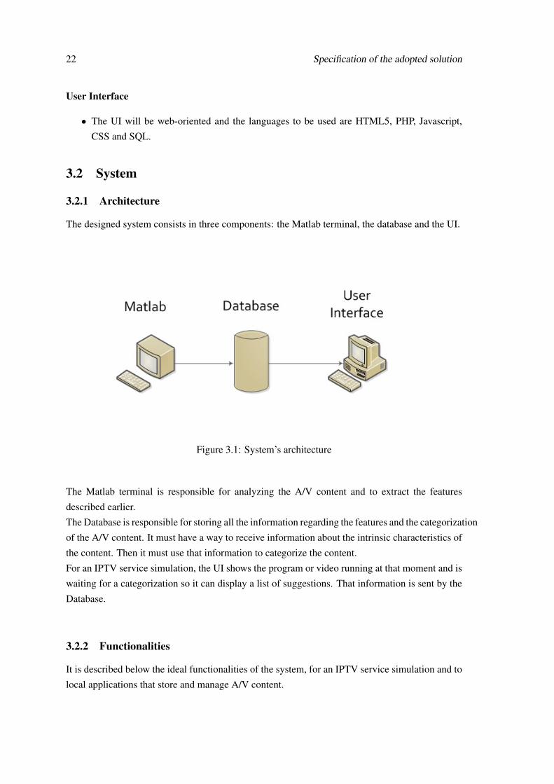
The designed system consists in three components: the Matlab terminal, the database and the UI.
Figure 3.1: System’s architecture
The Matlab terminal is responsible for analyzing the A/V content and to extract the features
described earlier.
The Database is responsible for storing all the information regarding the features and the categorization
of the A/V content. It must have a way to receive information about the intrinsic characteristics of
the content. Then it must use that information to categorize the content.
For an IPTV service simulation, the UI shows the program or video running at that moment and is
waiting for a categorization so it can display a list of suggestions. That information is sent by the
Database.
3.2.2 Functionalities
It is described below the ideal functionalities of the system, for an IPTV service simulation and to
local applications that store and manage A/V content.
3.2 System 23
IPTV service
• No user input;
• Analyze the A/V content (feature extraction) in real time;
• Categorize the A/V content;
• Allow the user to view the suggestions to the current A/V content.
Local applications
• May allow user input;
• Analyze the A/V content (feature extraction)
• Categorize the A/V content;
• Allow the user to view the suggestions to the current A/V content;
• Allow the user to view the list of recognized faces in the content;
• Allow the user to view the list of non-recognized faces in the content for possible manual
attribution.

24 Specification of the adopted solution
Chapter 4
Development
This chapter describes the work developed along the course of the dissertation. It is presented the
work developed on each block of the designed system, as well as the obtained results.
4.1 Overview
4.1.1 Database
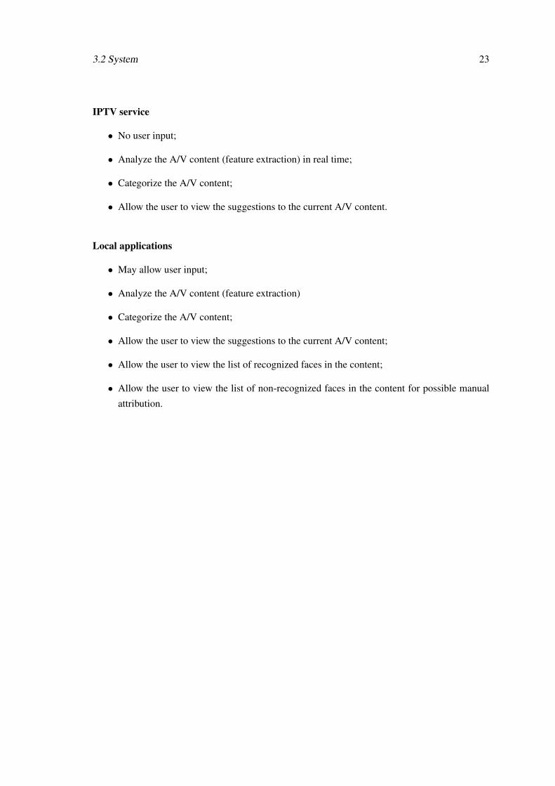
The database is composed by 3 associations: Movie, Person and Genre, as presented on figure 4.1.
File contains information about the features extracted from the A/V content.
Person contains information about any person detected during the analysis.
Genre contains the information (A/V features) that represent the content.
Figure 4.1: Entity-Association model
25

26 Development
4.1.2 Matlab
Shot boundaries detection algorithm
To extract some of the A/V features, it is mandatory to retrieve the boundaries of the scenes that
compose the video.
The transition between scenes is given by hard cuts, fades or dissolves, being the last the most
unused. For that reason, the attention was given to detect hard cuts and fades.
• Fades
As fades are usually understandable as transitions from a scene to a black or white background or
vice-versa, the criteria used to detect them is color. Black and white are formed by the combination
of RGB as (0,0,0) and (255,255,255), respectively. The algorithm to detect both transitions is
described in figure 4.2. As we are referring to fades, it wouldn’t be recommended that the value
criteria for RGB would be (0,0,0) and (255,255,255) as it could possibly not reach perfect black or
white backgrounds, and even if it does, avoids the algorithm to enter on the detection phase only
once. By using (5,5,5) and (250, 250, 250), there is a small margin to help the algorithm get a
better performance.
Figure 4.2: Fades detection criteria

4.1 Overview 27
• Hard Cuts
Hard cuts are perceived as complete alteration of the image displayed on a certain time of the
movie. By using color difference between frames, it is possible to detect those changes. This
value is obtained by subtracting the red, green and blue average values from the current frame
with the previous one. As the calculations are made frame by frame, it is impossible to classify
one frame as a hard cut boundary without computing the next. It is important to note that color
difference between frames may mean that the previous frame can be a part of a fade transition
(even though this isn’t the criteria) so it is necessary to prevent that situation. It is possible in some
rare occasions to obtain consecutive frames with a color difference above the threshold used, which
needs again extra precaution.
Special Effects (SFX) during scenes and camera motion are factors to consider as they will most
likely represent a considerable color variation between frames, giving false positive hard cuts.
It is defined that a scene has the minimum duration of 1 second to avoid possible false positives.
On the figure 4.3, it is described summarily the developed algorithm.
Figure 4.3: Hard cuts detection criteria

28 Development
Motion
To calculate the motion feature between scenes, it is performed edge detection for every frame
to isolate objects of interest. It is used the Sobel operator to calculate the magnitude of the
gradient. The image is then transformed to black and white to get better definition on the edges,
and it is calculated the difference between consecutive frames to obtain an image that represents
the movement of the objects of interest. This is achieved by using the appropriate function on
MATLAB (im2bw). This funcion finds the most suitable threshold that separates the best the
image’s histogram and then assign the intensity values to ’0’ or ’1’ accordingly. To interpret the
information this image gives, it is calculated the sum of ’1’ of the matrix, that represent the pixels
that suffered transformations from ’0’ to ’1’ and vice-versa, being then divided by the size of the
matrix (lines*columns) to obtain the percentage of modified pixel values.
Figure 4.4: Sobel gradient output
Face Detection
Face detection is obtained using the Vision toolbox available on Matlab. The CascadeObjectDetector
is a object detector that uses the Viola-Jones algorithm and by default is configured to detect faces.
As some tests were made, the algorithm was capable of detecting faces correctly if they were on
a sufficient good angle with the camera. Sometimes the algorithm provided false detections, and
to avoid the majority of those situations, it was defined a condition of only accepting the face that
fills the biggest percentage of the image.
Figure 4.5: Example of face detection

4.1 Overview 29
Face Recognition
Face recognition was achieved through the Eigenfaces method.
The first step was to create the training set of images. Those were required to have the person
facing the camera and approximately the same lighting conditions. For that reason, it was necessary
to access images that fulfilled those requirements, and the solution was to use images of a sports
website, where the players took photos under the same conditions.
Figure 4.6: Training set of images
The average face was computed and it was possible to extract the unique features of each image
on the training set.
Figure 4.7: Average face of the training set of images
Figure 4.8: Example of an image’s features

30 Development
The covariance matrix was computed and its best eigenvectors extracted according to the eigenvalues.
The weights matrix, was formed and the algorithm is now ready to compute: random images and
repeat all the process or its weight vector to compare to the weights matrix. Based on the euclidean
distance, it’s decided if it’s a face and if it matches any of the faces of the training set or not.
4.1.3 Interface
The interface was designed to simulate an environment in which the user is able to watch a random
A/V content and after some time, it is presented a list of suggestions of other contents connected
to whatever he is watching at that time.
Figure 4.9: UI main page - analyzing content
It is defined that the analyzis of the content will last 5 minutes before the UI displays the list
of suggestions. After that time, the status will indicate that the results are ready, and by simply
pressing a button, the list will pop-out.

4.1 Overview 31
Figure 4.10: UI main page - results ready
Figure 4.11: List of suggestions after 5 minutes. Genre suggested is action, which is incorrect
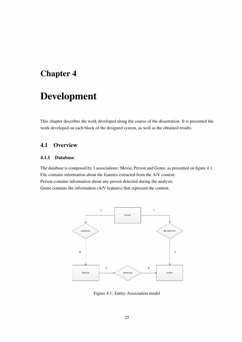
To get some feedback on the quality of the list displayed, the user has the option to accept or reject
the suggestions. If it is rejected, the content will be analyzed for 5 more minutes , in a total of 10.
This allows a possible better list of suggestions as the probability of the features converging to the
values that characterize their genre is bigger.
32 Development
Figure 4.12: List of suggestions after 10 minutes. Genre suggested is horror, which is correct
4.2 Results
4.2.1 Shot boundaries detection algorithm
To assure the algorithm performance on fade transitions, tests were made on clips containings only
fade to black and fade to white transitions. On both cases the output was the expected, with 100%
of the transitions detected and the number of scenes counted correctly.
Discovering the best threshold for the detection of hard cuts is very important and its value is
obtained resorting to machine learning classifiers described on chapter 2.
The dataset is formed by the color difference difference between the frames. There were used 3
different clips and the boundaries were detected visually and classified as such for each frame. All
the tests were made with the default values on the WEKA software, with 10-fold cross-validation
and the output for the 3 clips is shown on Appendix A.
Analyzing the output from the classifiers, the percentages of correctly classified instances are
above 97%, which leads to the conclusion that the color difference criteria is in fact a good
measurement for shot boundaries detection.
The threshold values for the decision trees on the 3 clips are mostly in the region of [5,15]. Chosing
a value close to 5 may induce the detection of false boundaries in cases of camera motion or SFX,
while a value close to 15 may not detect boundaries in frames which the color difference is not that
pronounced. For those reasons, it was decided to chose a middle term value, 10% for the criteria
of shot boundaries detection.
Tests were made on 2 clips containing all the type of transitions. To simulate all the possible
scenarios, one of the chosen clips was a fast paced series/movies trailer while the other clip was
slow paced, containing important information such as camera motion.
The output for the boundaries detection algorithm is shown on table 4.1.
4.2 Results 33
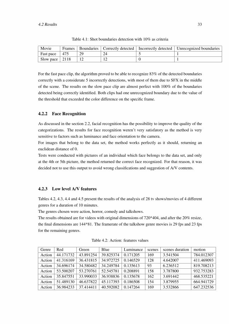
Table 4.1: Shot boundaries detection with 10% as criteria
Movie Frames Boundaries Correctly detected Incorrectly detected Unrecognized boundariesFast pace 475 29 24 5 1Slow pace 2118 12 12 0 1
For the fast pace clip, the algorithm proved to be able to recognize 83% of the detected boundaries
correctly with a considerate 5 incorrectly detections, with most of them due to SFX in the middle
of the scene. The results on the slow pace clip are almost perfect with 100% of the boundaries
detected being correctly identified. Both clips had one unrecognized boundary due to the value of
the threshold that exceeded the color difference on the specific frame.
4.2.2 Face Recognition
As discussed in the section 2.2, facial recognition has the possibility to improve the quality of the
categorizations. The results for face recognition weren’t very satisfatory as the method is very
sensitive to factors such as luminance and face orientation to the camera.
For images that belong to the data set, the method works perfectly as it should, returning an
euclidean distance of 0.
Tests were conducted with pictures of an individual which face belongs to the data set, and only
at the 4th or 5th picture, the method returned the correct face recognized. For that reason, it was
decided not to use this output to avoid wrong classifications and suggestion of A/V contents.
4.2.3 Low level A/V features
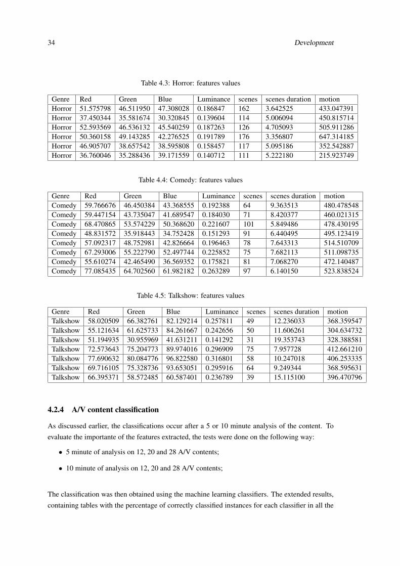
Tables 4.2, 4.3, 4.4 and 4.5 present the results of the analysis of 28 tv shows/movies of 4 different
genres for a duration of 10 minutes.
The genres chosen were action, horror, comedy and talkshows.
The results obtained are for videos with original dimensions of 720*404, and after the 20% resize,
the final dimensions are 144*81. The framerate of the talkshow genre movies is 29 fps and 23 fps
for the remaining genres.
Table 4.2: Action: features values
Genre Red Green Blue Luminance scenes scenes duration motionAction 44.171732 43.891254 39.825374 0.171205 169 3.541504 784.012307Action 41.316169 36.431815 34.972725 0.146529 128 4.642007 411.469093Action 34.696174 34.580482 34.249784 0.135613 93 6.236512 819.708213Action 53.500207 53.270761 52.545781 0.208891 158 3.787800 932.753283Action 35.847551 33.990033 36.938836 0.135678 162 3.691442 468.535221Action 51.489130 46.637822 45.117393 0.186508 154 3.879955 664.941729Action 36.984233 37.414411 40.592082 0.147264 169 3.532866 647.232536
34 Development
Table 4.3: Horror: features values
Genre Red Green Blue Luminance scenes scenes duration motionHorror 51.575798 46.511950 47.308028 0.186847 162 3.642525 433.047391Horror 37.450344 35.581674 30.320845 0.139604 114 5.006094 450.815714Horror 52.593569 46.536132 45.540259 0.187263 126 4.705093 505.911286Horror 50.360158 49.143285 42.276525 0.191789 176 3.356807 647.314185Horror 46.905707 38.657542 38.595808 0.158457 117 5.095186 352.542887Horror 36.760046 35.288436 39.171559 0.140712 111 5.222180 215.923749
Table 4.4: Comedy: features values
Genre Red Green Blue Luminance scenes scenes duration motionComedy 59.766676 46.450384 43.368555 0.192388 64 9.363513 480.478548Comedy 59.447154 43.735047 41.689547 0.184030 71 8.420377 460.021315Comedy 68.470865 53.574229 50.368620 0.221607 101 5.849486 478.430195Comedy 48.831572 35.918443 34.752428 0.151293 91 6.440495 495.123419Comedy 57.092317 48.752981 42.826664 0.196463 78 7.643313 514.510709Comedy 67.293006 55.222790 52.497744 0.225852 75 7.682113 511.098735Comedy 55.610274 42.465490 36.569352 0.175821 81 7.068270 472.140487Comedy 77.085435 64.702560 61.982182 0.263289 97 6.140150 523.838524
Table 4.5: Talkshow: features values
Genre Red Green Blue Luminance scenes scenes duration motionTalkshow 58.020509 66.382761 82.129214 0.257811 49 12.236033 368.359547Talkshow 55.121634 61.625733 84.261667 0.242656 50 11.606261 304.634732Talkshow 51.194935 30.955969 41.631211 0.141292 31 19.353743 328.388581Talkshow 72.573643 75.204773 89.974016 0.296909 75 7.957728 412.661210Talkshow 77.690632 80.084776 96.822580 0.316801 58 10.247018 406.253335Talkshow 69.716105 75.328736 93.653051 0.295916 64 9.249344 368.595631Talkshow 66.395371 58.572485 60.587401 0.236789 39 15.115100 396.470796
4.2.4 A/V content classification
As discussed earlier, the classifications occur after a 5 or 10 minute analysis of the content. To
evaluate the importante of the features extracted, the tests were done on the following way:
• 5 minute of analysis on 12, 20 and 28 A/V contents;
• 10 minute of analysis on 12, 20 and 28 A/V contents;
The classification was then obtained using the machine learning classifiers. The extended results,
containing tables with the percentage of correctly classified instances for each classifier in all the

4.2 Results 35
tests as well as all the decision trees obtained are shown on appendix A.
When the full sample size is used, the 28 videos, the classifier with the best performance is the
J48 (60.7143%). Inspecting the 5 minutes decision tree, it is possible to separate the 4 genres in
2 blocks(comedy+talkshow and horror+action) by using the number of scenes as the key feature.
The scenes average duration and the blue color component separate all the 4 genres.
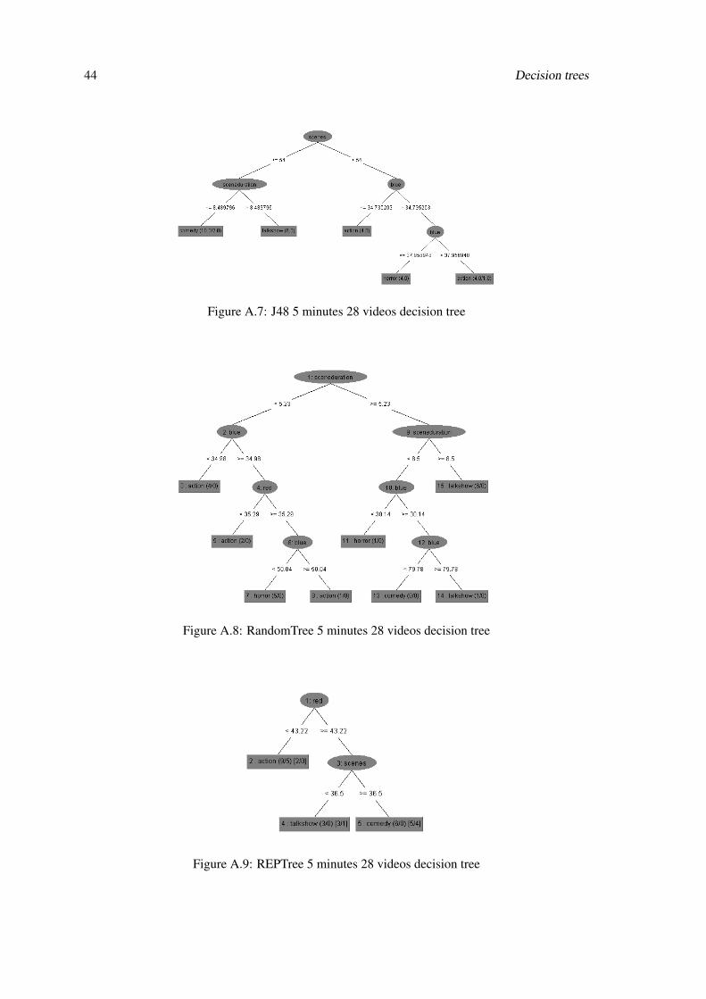
Figure 4.13: J48 5 minutes 28 videos decision tree
These are expected results, as 5 minutes is a short period of time to develop more unique values to
the features. The number of scenes and their average duration is the expected major classification
feature in this period of time, as talkshows and comedy tv-shows clearly show a slower pace than
action and horror tv-shows. The blue component doesn’t classify well enough either action or
horror tv-shows: from 7 action videos, 4 were correctly classified and 3 were classified as horror;
from 6 horror videos, 2 were classified correctly, 3 were classified as action and 1 as comedy.
The scene duration produces a better output: from 8 comedy videos, 5 were correctly classified, 2
were considered talkshows and 1 horror; from 7 talkshow videos, 6 were correctly classified and
1 classified as comedy.
36 Development
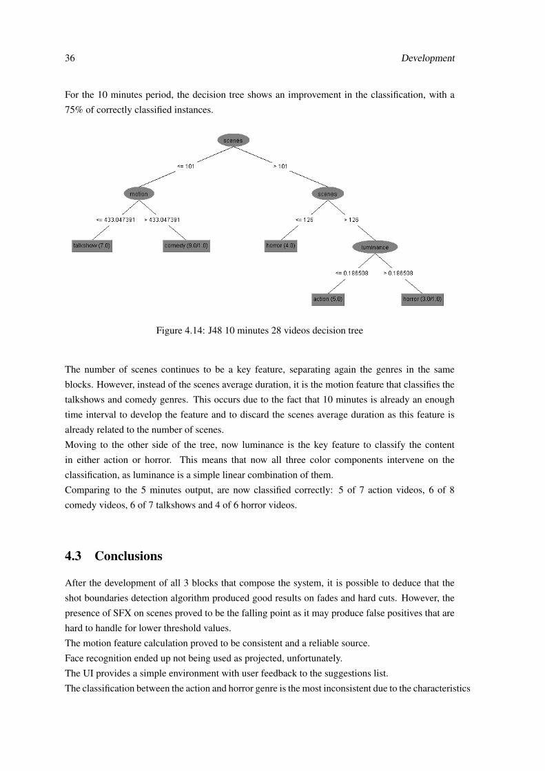
For the 10 minutes period, the decision tree shows an improvement in the classification, with a
75% of correctly classified instances.
Figure 4.14: J48 10 minutes 28 videos decision tree
The number of scenes continues to be a key feature, separating again the genres in the same
blocks. However, instead of the scenes average duration, it is the motion feature that classifies the
talkshows and comedy genres. This occurs due to the fact that 10 minutes is already an enough
time interval to develop the feature and to discard the scenes average duration as this feature is
already related to the number of scenes.
Moving to the other side of the tree, now luminance is the key feature to classify the content
in either action or horror. This means that now all three color components intervene on the
classification, as luminance is a simple linear combination of them.
Comparing to the 5 minutes output, are now classified correctly: 5 of 7 action videos, 6 of 8
comedy videos, 6 of 7 talkshows and 4 of 6 horror videos.
4.3 Conclusions
After the development of all 3 blocks that compose the system, it is possible to deduce that the
shot boundaries detection algorithm produced good results on fades and hard cuts. However, the
presence of SFX on scenes proved to be the falling point as it may produce false positives that are
hard to handle for lower threshold values.
The motion feature calculation proved to be consistent and a reliable source.
Face recognition ended up not being used as projected, unfortunately.
The UI provides a simple environment with user feedback to the suggestions list.
The classification between the action and horror genre is the most inconsistent due to the characteristics

4.3 Conclusions 37
that define them aren’t so much apart, as the action videos selected belong to a tv-show that
contains a lot of night scenes and low values of RGB.

38 Development
Chapter 5
Conclusions and future work
This chapter describes a global view about the achievements and an evaluation of the final product
versus the expected on the beginning of the work.
It is discussed the limitations of the developed system, the improvements to be made and some
possible routes to follow to improve it.
5.1 Conclusions
The main objective for this dissertation was to develop tools to classify and suggest A/V content
based on its intrinsic features. Although this was achieved, it needs to be taken in consideration
that the final results are based on a very small sample size of videos. Analyzing 28 videos for 10
minutes each isn’t enough to develop a solid classification.
From the analysis of the features, it was possible to verify that combinations of their values relate
to specific genres as expected.
The facial recognition method ended up not being used because its performance was rather poor
and it would end up helping classifying incorrectly the content. As the method is very sensitive
to the environment in which the faces from the data set were taken, when a random face needs
to be recognized and it was taken on a total different environment, it will most likely fail to
be recognized. A possible solution to this matter is to realize an image equalization (histogram
equalization).
5.2 Future work
From the work developed and described on this dissertation, here are some suggestions for possible
improvements:
• Facial recognition may provide extra information on the classification and suggestion of
A/V content;
• Shot boundaries detection: it is worth to try to reduce the false positives caused by SFX;
39

40 Conclusions and future work
• Improve the machine learning classifiers: all the classifications on WEKA were made using
default values;
• The user feedback system only analyzes the content for 5 more minutes. It could be
interesting to provide another suggestions based on previous answers by other users;
• Adding sound analysis is another possibility. This idea has the same principle as facial
recognition as it may be possible to relate sounds/songs to a certain content that belongs to
a certain genre.

Appendix A
Decision trees
This chapter presents the output of the machine learning classifiers. It contains information about
the shot boundaries threshold and the content classification.
A.1 Decision Trees - A/V content clasification
A.1.1 5 minutes
Table A.1: Correctly classified instances - 5 minutes 12 videos
Classifier % Correctly ClassifiedDecisionStump 0J48 41.6667Random Tree 41.6667REPTree 0
Table A.2: Correctly classified instances - 5 minutes 20 videos
Classifier % Correctly ClassifiedDecisionStump 45J48 45Random Tree 60REPTree 35
Table A.3: Correctly classified instances - 5 minutes 28 videos
Classifier % Correctly ClassifiedDecisionStump 50J48 60.7143Random Tree 42.8571REPTree 53.5714
41
42 Decision trees
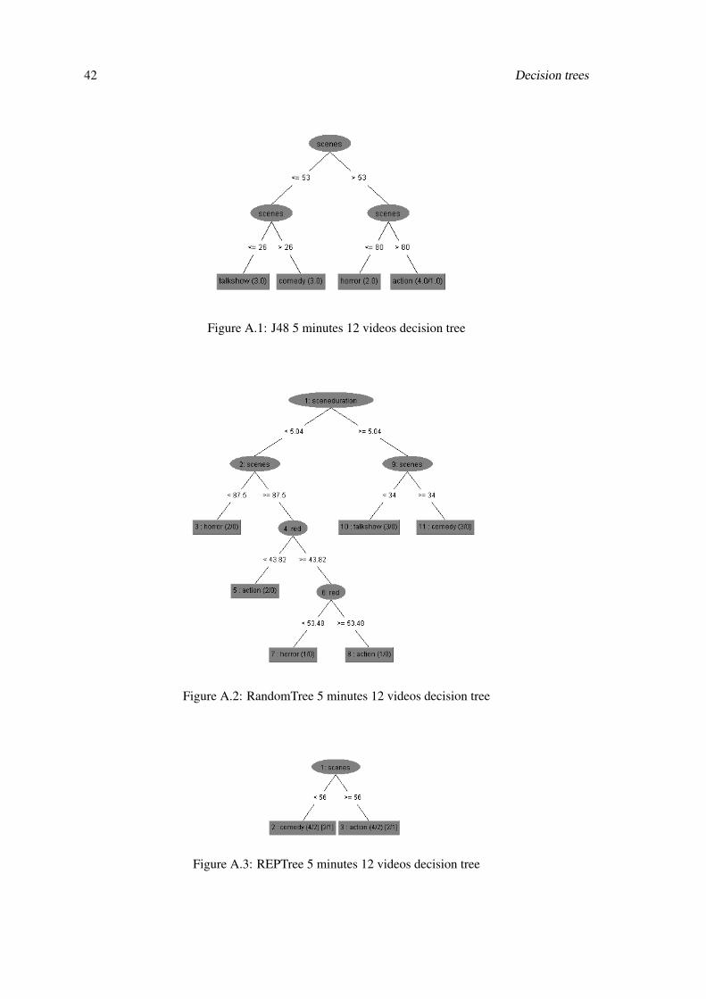
Figure A.1: J48 5 minutes 12 videos decision tree
Figure A.2: RandomTree 5 minutes 12 videos decision tree
Figure A.3: REPTree 5 minutes 12 videos decision tree
A.1 Decision Trees - A/V content clasification 43
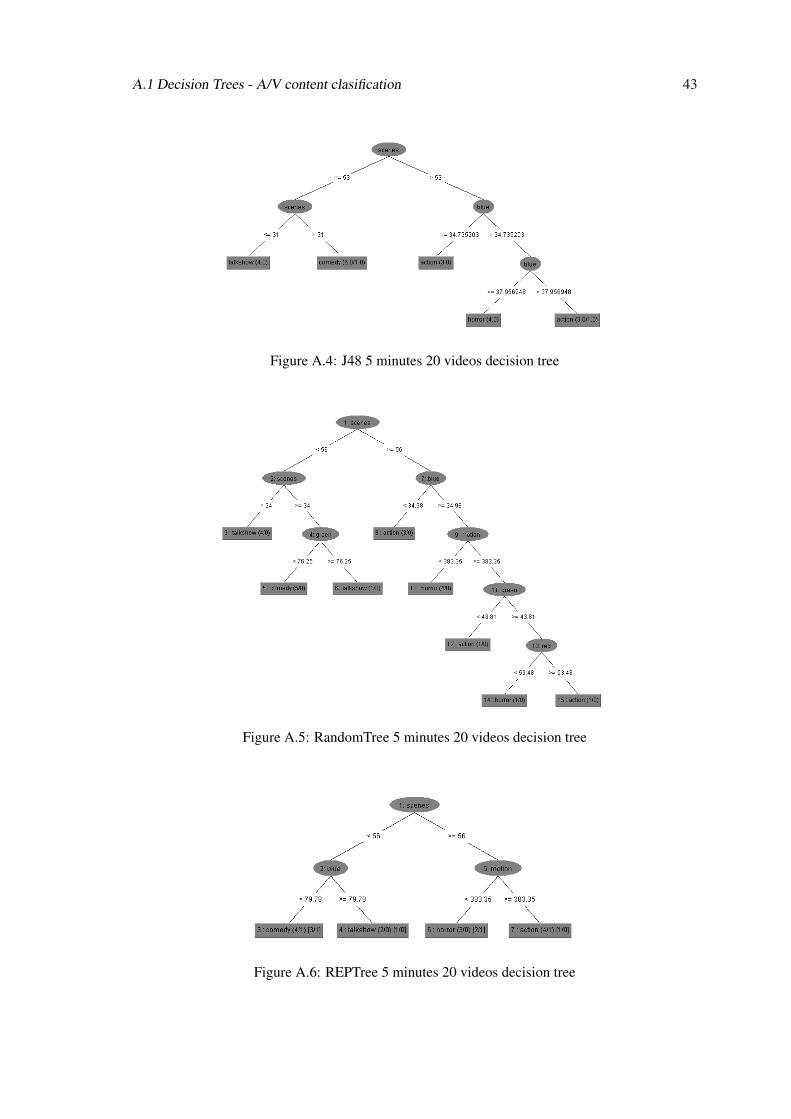
Figure A.4: J48 5 minutes 20 videos decision tree
Figure A.5: RandomTree 5 minutes 20 videos decision tree
Figure A.6: REPTree 5 minutes 20 videos decision tree
44 Decision trees
Figure A.7: J48 5 minutes 28 videos decision tree
Figure A.8: RandomTree 5 minutes 28 videos decision tree
Figure A.9: REPTree 5 minutes 28 videos decision tree

A.1 Decision Trees - A/V content clasification 45
A.1.2 10 minutes
46 Decision trees
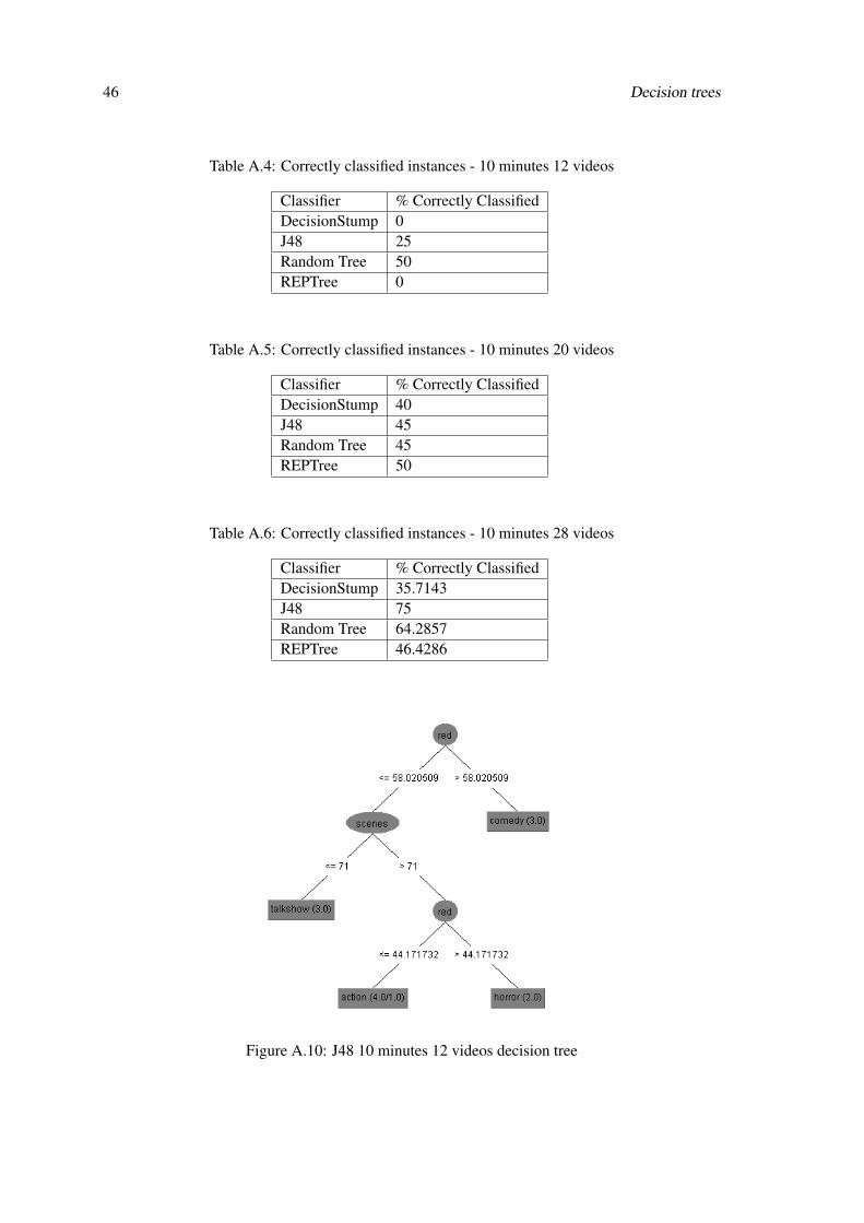
Table A.4: Correctly classified instances - 10 minutes 12 videos
Classifier % Correctly ClassifiedDecisionStump 0J48 25Random Tree 50REPTree 0
Table A.5: Correctly classified instances - 10 minutes 20 videos
Classifier % Correctly ClassifiedDecisionStump 40J48 45Random Tree 45REPTree 50
Table A.6: Correctly classified instances - 10 minutes 28 videos
Classifier % Correctly ClassifiedDecisionStump 35.7143J48 75Random Tree 64.2857REPTree 46.4286
Figure A.10: J48 10 minutes 12 videos decision tree
A.1 Decision Trees - A/V content clasification 47
Figure A.11: RandomTree 10 minutes 12 videos decision tree
Figure A.12: REPTree 10 minutes 12 videos decision tree

48 Decision trees
Figure A.13: J48 10 minutes 20 videos decision tree
Figure A.14: RandomTree 10 minutes 20 videos decision tree

A.1 Decision Trees - A/V content clasification 49
Figure A.15: REPTree 10 minutes 20 videos decision tree
Figure A.16: J48 10 minutes 28 videos decision tree
Figure A.17: RandomTree 10 minutes 28 videos decision tree

50 Decision trees
Figure A.18: REPTree 10 minutes 28 videos decision tree

A.2 Decision Trees - shot boundaries 51
A.2 Decision Trees - shot boundaries
52 Decision trees
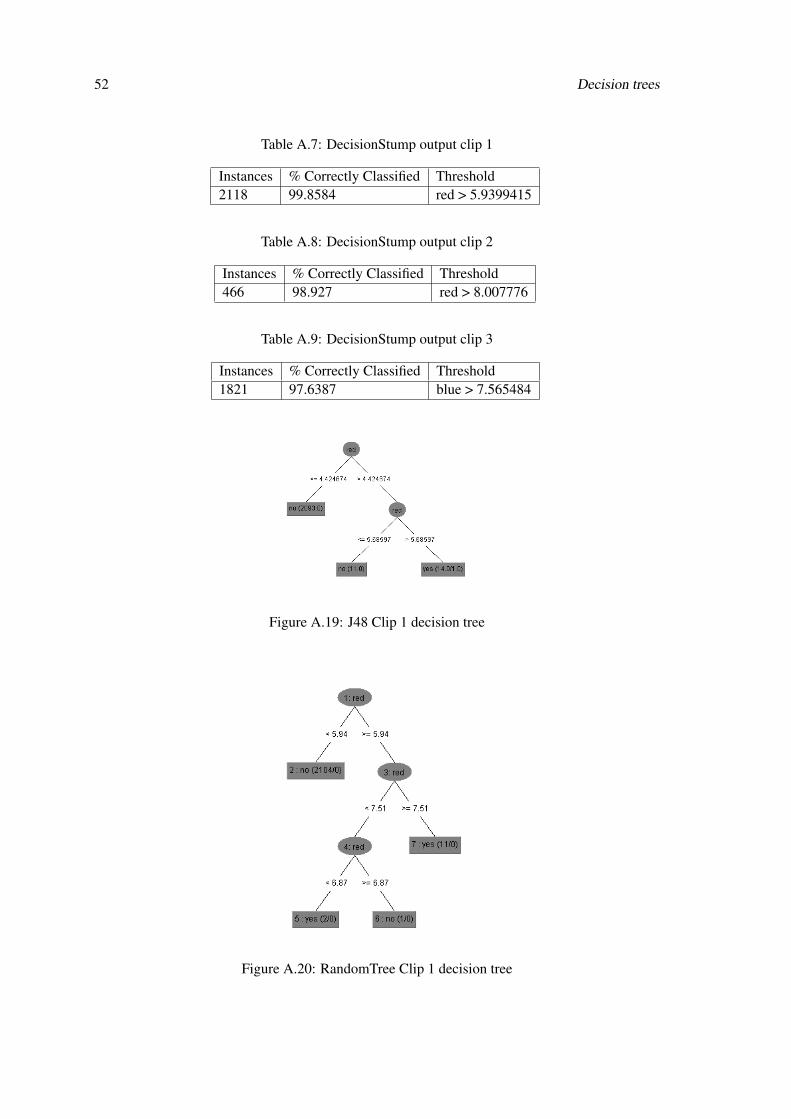
Table A.7: DecisionStump output clip 1
Instances % Correctly Classified Threshold2118 99.8584 red > 5.9399415
Table A.8: DecisionStump output clip 2
Instances % Correctly Classified Threshold466 98.927 red > 8.007776
Table A.9: DecisionStump output clip 3
Instances % Correctly Classified Threshold1821 97.6387 blue > 7.565484
Figure A.19: J48 Clip 1 decision tree
Figure A.20: RandomTree Clip 1 decision tree

A.2 Decision Trees - shot boundaries 53
Figure A.21: REPTree Clip 1 decision tree
Figure A.22: J48 Clip 2 decision tree
Figure A.23: RandomTree Clip 2 decision tree
54 Decision trees
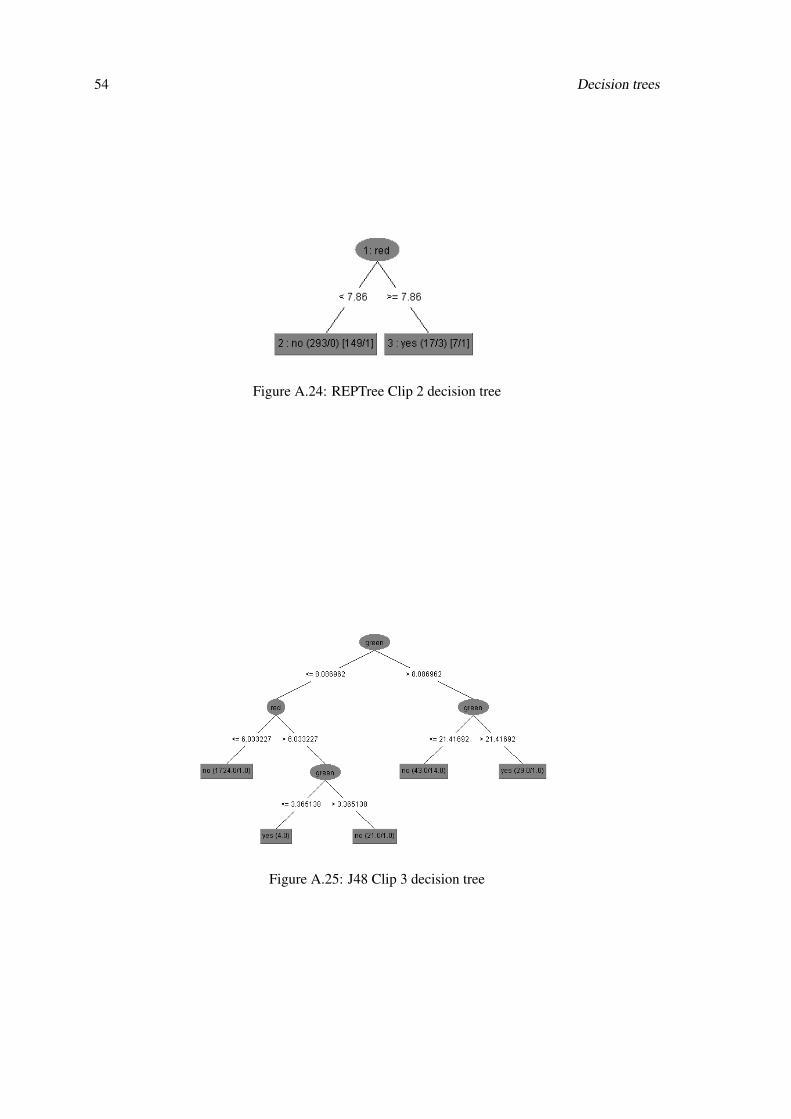
Figure A.24: REPTree Clip 2 decision tree
Figure A.25: J48 Clip 3 decision tree
A.2 Decision Trees - shot boundaries 55
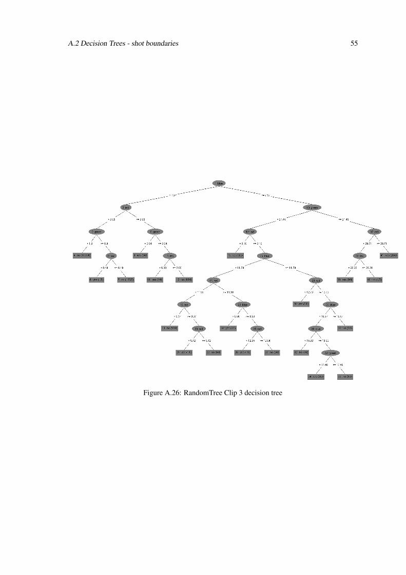
Figure A.26: RandomTree Clip 3 decision tree
56 Decision trees
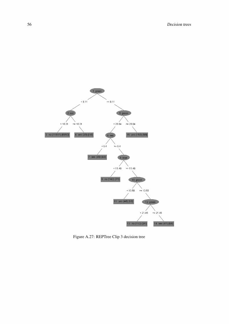
Figure A.27: REPTree Clip 3 decision tree

Bibliography
[1] Huang, Hui-Yu, Weir-Sheng Shih, and Wen-Hsing Hsu. "Film classification based on
low-level visual effect features." Journal of Electronic Imaging 17.2 (2008): 023011-023011.
[2] Smith, Mark, Ray Hashemi, and Leslie Sears. "Classification of Movies and Television
Shows Using Motion." Information Technology: New Generations, 2009. ITNG’09. Sixth
International Conference on. IEEE, 2009.
[3] Boreczky, John S., and Lawrence A. Rowe. "Comparison of video shot boundary detection
techniques." Journal of Electronic Imaging 5.2 (1996): 122-128.
[4] Zabih, Ramin, Justin Miller, and Kevin Mai. "A feature-based algorithm for detecting and
classifying production effects." Multimedia systems 7.2 (1999): 119-128.
[5] Lienhart, Rainer W. "Comparison of automatic shot boundary detection algorithms."
Electronic Imaging’99. International Society for Optics and Photonics, 1998.
[6] Image Segmentation I Last Access on January 2014
https://oldmoodles.fe.up.pt/1213/pluginfile.php/30043/mod_resource/content/2/Lectures/
AIBI-ImageSegmentation_2012-13_Part1.pdf
[7] Otsu, Nobuyuki. "A threshold selection method from gray-level histograms."Automatica
11.285-296 (1975): 23-27.
[8] Image Segmentation II Last Access on January 2014
https://oldmoodles.fe.up.pt/1213/pluginfile.php/30044/mod_resource/content/3/Lectures/
AIBI-ImageSegmentation_part2_2012-13.pdf
[9] Edge Corner Detection Last Access on January 2014
https://oldmoodles.fe.up.pt/1213/pluginfile.php/30044/mod_resource/content/3/Lectures/
AIBI-ImageSegmentation_part2_2012-13.pdf
[10] Gurumurthy, Sasikumar, and B. K. Tripathy. "Design and Implementation of Face
Recognition System in Matlab Using the Features of Lips." International Journal of Intelligent
Systems and Applications (IJISA) 4.8 (2012): 30.
[11] Nilsson, Viktor, and Amaru Ubillus. "Face Recognition in Color Images using Matlab
TNM034, Linköpings University." (2012).
57

58 BIBLIOGRAPHY
[12] M. Turk and A. Pentland, "Eigenfaces for Recognition", Journal of Cognitive
Neuroscience,vol.3, no. 1, pp. 71-86, 1991, hard copy.
[13] Kim, Kyungnam. "Face recognition using principle component analysis." International
Conference on Computer Vision and Pattern Recognition. 1996.
[14] Ozer, Patrick. "Data Mining Algorithms for Classification." (2008).
[15] Frank, Eibe, et al. "Data mining in bioinformatics using Weka."Bioinformatics 20.15 (2004):
2479-2481.