Catchment modeling and model transferability in upper … · ity in upper Blue Nile Basin, Lake...

HAL Id: hal-00298937https://hal.archives-ouvertes.fr/hal-00298937

Submitted on 20 Mar 2008

HAL is a multi-disciplinary open accessarchive for the deposit and dissemination of sci-entific research documents, whether they are pub-lished or not. The documents may come fromteaching and research institutions in France orabroad, or from public or private research centers.

L’archive ouverte pluridisciplinaire HAL, estdestinée au dépôt et à la diffusion de documentsscientifiques de niveau recherche, publiés ou non,émanant des établissements d’enseignement et derecherche français ou étrangers, des laboratoirespublics ou privés.

Catchment modeling and model transferability in upperBlue Nile Basin, Lake Tana, Ethiopia

A. S. Gragne, S. Uhlenbrook, Y. Mohammed, S. Kebede

To cite this version:A. S. Gragne, S. Uhlenbrook, Y. Mohammed, S. Kebede. Catchment modeling and model transferabil-ity in upper Blue Nile Basin, Lake Tana, Ethiopia. Hydrology and Earth System Sciences Discussions,European Geosciences Union, 2008, 5 (2), pp.811-842. <hal-00298937>

https://hal.archives-ouvertes.fr/hal-00298937

https://hal.archives-ouvertes.fr

HESSD

5, 811–842, 2008

Catchment modeling

in upper Blue Nile,

Ethiopia

A. S. Gragne et al.

Title Page

Abstract Introduction

Conclusions References

Tables Figures

◭ ◮

◭ ◮

Back Close

Full Screen / Esc

Printer-friendly Version

Interactive Discussion

Hydrol. Earth Syst. Sci. Discuss., 5, 811–842, 2008

www.hydrol-earth-syst-sci-discuss.net/5/811/2008/

© Author(s) 2008. This work is distributed under

the Creative Commons Attribution 3.0 License.

Hydrology andEarth System

SciencesDiscussions

Papers published in Hydrology and Earth System Sciences Discussions are under

open-access review for the journal Hydrology and Earth System Sciences

Catchment modeling and model

transferability in upper Blue Nile Basin,

Lake Tana, Ethiopia

A. S. Gragne1, S. Uhlenbrook

2,3, Y. Mohammed

4, and S. Kebede

5

1Dept. of Water Resources and Environmental Engineering, Jimma Univ., Jimma, Ethiopia

2UNESCO–IHE, Dept. of Water Engineering, P.O. Box 3015, 2601 DA Delft, The Netherlands

3Dept. of Water Resources, Delft University of Technology, P.O. Box 5048, 2600 GA Delft, The

Netherlands4International Water Management Institute (IWMI), Addis Ababa, Ethiopia

5Earth Sciences Department, Addis Ababa University, Addis Ababa, Ethiopia

Received: 15 February 2008 – Accepted: 15 February 2008 – Published: 20 March 2008

Correspondence to: S. Uhlenbrook ([email protected])

Published by Copernicus Publications on behalf of the European Geosciences Union.

811

http://www.hydrol-earth-syst-sci-discuss.net

http://www.hydrol-earth-syst-sci-discuss.net/5/811/2008/hessd-5-811-2008-print.pdf

http://www.hydrol-earth-syst-sci-discuss.net/5/811/2008/hessd-5-811-2008-discussion.html

http://creativecommons.org/licenses/by/3.0/

HESSD

5, 811–842, 2008

Catchment modeling

in upper Blue Nile,

Ethiopia

A. S. Gragne et al.

Title Page



Tables Figures

◭ ◮

◭ ◮

Back Close

Full Screen / Esc



Abstract

Understanding spatial and temporal distribution of water resources has an important

role for water resource management. To understand water balance dynamics and

runoff generation mechanisms at the Gilgel Abay catchment (a major tributary into lake

Tana, source of Blue Nile, Ethiopia) and to evaluate model transferability, catchment5

modeling was conducted using the conceptual hydrological model HBV. The catchment

of the Gigel Abay was sub-divided into two gauged sub-catchments (Upper Gilgel Abay,

UGASC, and Koga, KSC) and one ungauged sub-catchment.

Manual calibration of the daily models for three different catchment representations

(CRs): (i) lumped, (ii) lumped with multiple vegetation zones, and (iii) semi-distributed10

with vegetations zone and elevation zones, showed good to satisfactory model perfor-

mance (Nash-Sutcliffe efficiency values, Reff>0.75 and >0.6, respectively, for UGASC

and KSC). The change of the time step to fifteen and thirty days resulted in very good

model performances in both sub-catchments (Reff>0.8). The model parameter trans-

ferability tests conducted on the daily models showed poor performance in both sub-15

catchments, whereas the fifteen and thirty days models yielded high Reff values using

transferred parameter sets. This together with the sensitivity analysis carried out after

Monte Carlo simulations (1 000 000 model runs) per CR explained the reason behind

the difference in hydrologic behaviors of the two sub-catchments UGASC and KSC.

The dissimilarity in response pattern of the sub-catchments was caused by the pres-20

ence of dambos in KSC and differences in the topography between UGASC and KSC.

Hence, transferring model parameters from the view of describing hydrological process

was found to be not feasible for all models. On the other hand, from a water resources

management perspective the results obtained by transferring parameters of the larger

time step model were acceptable.25

812





HESSD

5, 811–842, 2008

Catchment modeling

in upper Blue Nile,

Ethiopia

A. S. Gragne et al.

Title Page



Tables Figures

◭ ◮

◭ ◮

Back Close

Full Screen / Esc



1 Introduction

The Nile Basin is shared by ten riparian countries and is the life source for more than

160 million people living in the basin. The Blue Nile, originating from the Ethiopian

Plateau, is the major source of the Nile water and contributes more than 80% of the Nile

flow during the wet season (Conway and Hulme, 1993; Mishra et al., 2003) and 64% of5

the water at Aswan in Egypt (El-Khodan, 2003). Similar to other sub-basins, irrigation,

hydropower power and flood management are the key water resource development

needs in Ethiopia and in the Nile region in general. Therefore, understanding the water

balance and its spatial and temporal dynamics in the headwaters is crucial.

A number of studies have been conducted on the Nile River; however, due to ab-10

sence of data and other priorities, few of them covered the hydrology of the Upper Blue

Nile. Most of the studies on the Blue Nile focus rather downstream, e.g., at Roseries

dam in Sudan (Johnson and Curtis, 1994). In the past few decades, some research

and development projects on the Upper Blue Nile were conducted (Lahmeyer, 1962;

USBR, 1964; JICA, 1997; BCEOM, 1999; Conway and Hume, 1993; Mishra et al.,15

2003; Kebede et al., 2005). The runoff estimations of Lake Tana’s sub-basin (source

of Blue Nile) were computed backward using observed lake outflows. This contributes

to the uncertainty of the runoff yield estimates into the Lake Tana (MoWR, 2005), and

subsequently to the future generated downstream flows. Generally, little is known about

the hydrology of the Gilgel Abay Catchment, one of the main tributaries of Lake Tana.20

The water balance studies of Lake Tana indicated that more than 93% of the inflow

to Lake Tana originates from four main tributary rivers: Gilgel Abay, Gumera, Rib and

Megech (Tarekegn and Tadege, 2005; Kebede et al., 2006). The Gilgel-Abay alone

contributes about 60% of the inflow to the lake (Tessema, 2006).

From operational water resources management point of view, hydrological models25

are crucial for understanding and predicting the spatial and temporal distribution of wa-

ter resources (e.g. Liden and Harlin, 2000; Uhlenbrook et al., 2004). This includes

predicting the future impacts of changes in the land use or the climate on hydrology.

813





HESSD

5, 811–842, 2008

Catchment modeling

in upper Blue Nile,

Ethiopia

A. S. Gragne et al.

Title Page



Tables Figures

◭ ◮

◭ ◮

Back Close

Full Screen / Esc



Catchment scale studies of the Gilgel-Abay should help to identify the water balance

dynamics, runoff generation processes and provide further insight on lake level fluctu-

ations that are important for the use of the lake water resources and the lake’s role in

moderating the flow of the Blue Nile River. The objective of this paper is to conduct

rainfall-runoff modeling, assess model complexity, and provide an overview on model5

transferability of the HBV model at different time-scale.

2 The study area

The Gilgel Abay catchment (GAC; 5000 km2) is the largest of the four main sub-

catchments of Lake Tana. It drains the southern part of the Lake Tana basin and has

two gauged sub-catchments, namely the Upper Gilgel Abay (UGASC) and Koga (KSC)10

of 1654 km2

and 307 km2, respectively (Fig. 1). With elevation ranging from 1787 m to

3524 m a.m.s.l., rugged mountainous topography characterizes the southern part of the

catchment and its periphery in the west and southeast, while the remaining part is a

typical low lying plateau with gentle slopes. The geology is composed of quaternary

basalts and alluviums. The soils are dominated by clays and clayey loams. The dom-15

inant land use units are agricultural (65.5%), agro-pastoral (33.4%), agro-sylvicultural

(1%) and urban (0.1%). Among these, rainfed agriculture covers 65% of the GAC, and

it amounts to 74% and 64% on the UGASC and KSC, respectively. Although there is

no fixed dependence between the land use and elevation through out the basin, oc-

currence of seasonal wetlands (dambos) is observed mainly in the gentle slope areas20

(Fig. 1); compared to UGASC, the dambo covers a larger area in KSC. As described

by von der Heyden and New (2003), the role of dambos in affecting catchment evap-

otranspiration, increasing base flow, and decreasing and retarding flood flow are not

fully understood.

The rainfall over the Gigel Abay and Upper Blue Nile in general, originates from25

moist air coming from Atlantic and Indian oceans following the north-south movement

of the Inter Tropical Convergence Zone (ITCZ). Different studies (e.g., Kebede et al.,

814





HESSD

5, 811–842, 2008

Catchment modeling

in upper Blue Nile,

Ethiopia

A. S. Gragne et al.

Title Page



Tables Figures

◭ ◮

◭ ◮

Back Close

Full Screen / Esc



2006; Tarekegn and Tadege, 2005) demonstrated that the study area has one main

rainy season between June and September, in which 70% to 90% of the annual total

rainfall occurs. Rainfall data from surrounding meteorological stations indicate signifi-

cant spatial variations of rainfall in the GAC following the topography, with a decreasing

trend from south to north. The temperature variations throughout the year are small5

(BCEOM, 1999). There are three discharge gauging stations (Fig. 1); all stations are

equipped with staff gauges and readings have been taken twice a day (at 06:00 and

18:00 local time).

3 Materials and methods

3.1 Data screening and filling of gaps10

The data to be used for hydrological simulations should be stationary, consistent and

homogeneous (Dahmen and Hall, 1990). Therefore, we first screened the hydro-

meteorological data in different steps: visual data screening and plausibility checks,

comparison of monthly and annual totals for the hydrological years, tests for absence of

trends, and split-record test for the stationarity of the mean and the variance. Records15

of nine rain gauges with various gaps were completed using regression and spatial

interpolation techniques. Different combinations of stations have been attempted for

filling the data gaps. After checking the quality of the point measurements and esti-

mation of aerial mean values, total monthly and annual time series of the estimated

rainfall, temperature and runoff data were tested for absence of trend, stability of vari-20

ance and stability of mean. Names and locations of all flow and rain gauge stations

used in this study, together with their respective lengths of data series and percentages

of missing data can be found in Table 1.

815





HESSD

5, 811–842, 2008

Catchment modeling

in upper Blue Nile,

Ethiopia

A. S. Gragne et al.

Title Page



Tables Figures

◭ ◮

◭ ◮

Back Close

Full Screen / Esc



3.2 The HBV model

3.2.1 Model description and input data

The widely used HBV model (Bergstrom, 1976) is a conceptual hydrological model,

which simulates discharge using as input variables of rainfall, temperature and esti-

mates of potential evaporation. The model consists of different routines representing5

snow accumulation and melt (not used for the study area), groundwater recharge and

actual evaporation as functions of actual water storage in a soil box, three runoff com-

ponents computed by three linear reservoir equations, and channel routing by a tri-

angular weighting function. Detailed model descriptions can be found elsewhere (e.g.

Bergstrom, 1995). The version of the model used in this study, “HBV light” (Seibert,10

2002), corresponds to the version HBV-6 described by Bergstrom (1992).

The input data used are daily areal rainfall and temperature estimates as well as

monthly estimates of potential evapotranspiration. Besides, in the absence of daily

potential evapotranspiration data, long-term daily mean temperature data was used

to adjust the long-term mean monthly evapotranspiration values to daily values (Lind-15

stroem et al., 1996). Aerial estimates of rainfall and temperature for GAC, UGASC

and KSC were calculated using the Thiessen polygon method. These values were dis-

tributed over elevation zones using elevation gradients (lapse rates). The estimation

of the monthly potential evapotranspiration, EO (mm/d), was done using the Penman-

Monteith equation. While estimating the potential evaporation of GAC, UGASC and20

KSC existence of different land cover units were taken into account. As described

by Chang (2003), when a grassland and forestland/woodland are subject to the same

meteorological conditions, the latter transpires more. However, because of absence

of data it was not possible to quantify the proportions of grassland and woodland, and

they were mapped as mixed grassland (major land use unit) by BCEOM (1999). Hence,25

in determining EO, the mixed grassland was considered to evaporate 10% more than

computed EO. Considering elevation zones and vegetation zones as primary hydrolog-

ical units during the distributed modeling, the catchments were delineated into these

816





HESSD

5, 811–842, 2008

Catchment modeling

in upper Blue Nile,

Ethiopia

A. S. Gragne et al.

Title Page



Tables Figures

◭ ◮

◭ ◮

Back Close

Full Screen / Esc



different zones using ArcGIS.

Different model structures were applied to investigate the impact of the model struc-

ture on the hydrological simulations and the model transferability. Therefore, all input

data were prepared for the following three catchment representations (CRs): (i) lumped

model structure (CR I), (ii) lumped model structure with up to three vegetation zones5

(CR II), and (iii) semi-distributed model structure with multiple elevation zones and up

to three vegetation zones per elevation zone (CR III). The catchment boundaries and

elevation zones were estimated using a 90×90 m2

DEM and resulted in 18, 16 and 12

elevation zones of 100 m intervals for the GAC, UGASC and KSC, respectively.

3.2.2 Model calibration, validation and performance assessment10

A manual model calibration was carried out, which was preceded by Monte Carlo sim-

ulations for every CR. However, quantifying the parameter uncertainty of the model, as

extensively demonstrated e.g. by Seibert (1997) or Uhlenbrook et al. (1999) in other

study areas, was beyond the scope of this paper. The model performance was assed

visually and statistically; the objectives during calibration were to maximize the model15

efficiency according to Nash and Sutcliffe (1970) and to minimize the volume error (i.e.

mean difference between simulated and observed runoff per year) at the same time. A

simple sensitivity analysis to identify the most sensitive model parameters was carried

out separately for each sub-catchment and CR. The number of model parameters used

for model calibration varied for UGASC and KSC and also for the three CRs (Table 2).20

Validations of the models were done by following a split-record test using data of the

periods 2000/2001 to 2004/2005 (UGASC) and 2001/2002 to 2004/2005 (KSC). By ap-

plying the best model parameter sets of one sub-catchment to the other sub-catchment

allowed to test the parameter transferability. Finally, comparison made between most

sensitive parameters of UGASC and KSC enabled differentiate hydrologic behaviors of25

the two sub-catchments.

817





HESSD

5, 811–842, 2008

Catchment modeling

in upper Blue Nile,

Ethiopia

A. S. Gragne et al.

Title Page



Tables Figures

◭ ◮

◭ ◮

Back Close

Full Screen / Esc



4 Data analysis

4.1 Preparation of hydrometeorological input data

After checking of the data quality and completing of missing hydrometeorological and

hydrological data, areal model input data were computed. The equations used for

estimating areal rainfall and temperature values of GAC, UGASC and KSC using the5

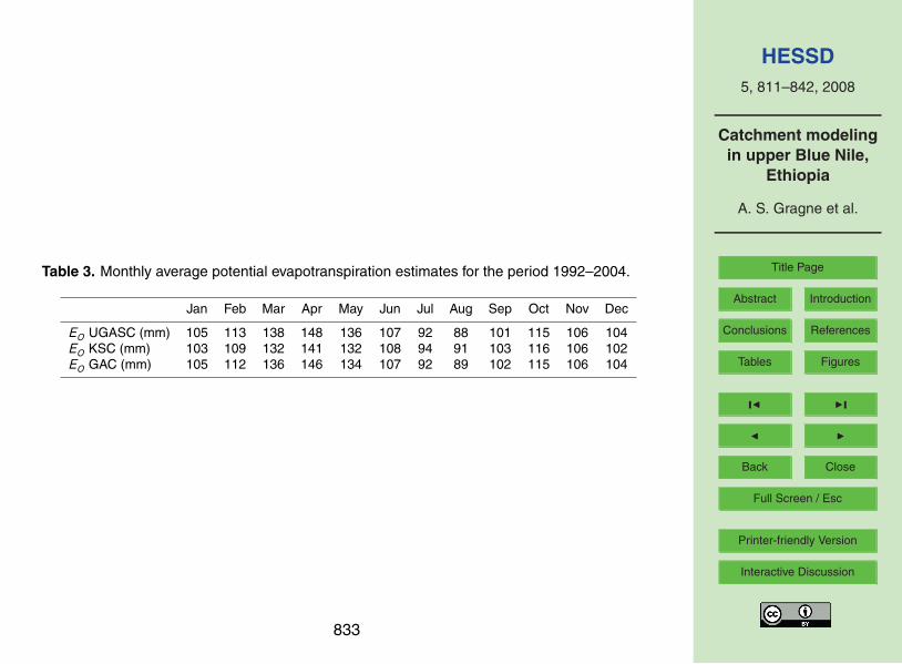
Thiessen polygon method are as given in Eqs. (1)–(6). The potential evapotranspiration

values calculated by considering the wighted mean values obtained for each land use

according to the Penman-Monteith equation are given in Table 3.

PAGAC = 0.08PZ + 0.17PAS + 0.41PWA + 0.08PD + 0.16PS + 0.1PG (1)

TAGAC = 0.07TZ + 0.17TAS + 0.43TWA + 0.08TD + 0.25TG (2)10

PAUGASC = 0.17PD + 0.21PG + 0.33PS + 0.29PWA (3)

TAUGASC = 0.36TWA + 0.17TD + 0.47PG (4)

PAKSC = 0.11PK + 0.11PS + 0.79PWA (5)

TAKSC = TWA (6)

The rainfall-elevation increases calculated based on long-term mean rainfall and eleva-15

tion data were estimated to 2.3% per 100 m (GAC) and 2.4% per 100 m (UGASC and

KSC). Similarly, the temperature-elevation lapse rate was determined to 0.14◦

C/100 m

and is applicable to all study catchments. The corresponding reference elevations for

the areal rainfall estimates were 2118 m (GAC), 2334 m (UGASC) and 2028 m (KSC).

The elevations of the mean temperatures were estimated to 2088 m (GAC), 2240 m20

(UGASC) and 1900 m (KSC).

818





HESSD

5, 811–842, 2008

Catchment modeling

in upper Blue Nile,

Ethiopia

A. S. Gragne et al.

Title Page



Tables Figures

◭ ◮

◭ ◮

Back Close

Full Screen / Esc



4.2 Statistical analysis

The time series analysis of the hydrometeorological data demonstrated inconsisten-

cies, instationarities and inhomogeneities for several monthly values before 1993. For

instance, the Pettitt test and F-test (significance level of 5%) applied to the monthly rain-

fall time series of GAC, UGASC and KSC identified two change points in June (19815

and 1988), and one change point for the March rainfall (1981). The conducted t-tests

exhibited changes in most of the months except July, December, January and February

in different years between 1981 and 1992. Similarly, annual aerial rainfall time series

showed change points in 1981, 1987 and 1990 for all three investigated catchments

(i.e. GAC, UGASC and KSC).10

Similar observations could be made for the discharge time series: the monthly dis-

charge revealed change points for the mean values in the years between 1981 and

1992 in all months except July and October (UGASC) and June, August and Decem-

ber (KSC). It was concluded that the change points and inconsistencies during the

earlier parts of the time series are likely to be caused by the poor data quality. As15

all inconsistencies, instationarities and inhomogeneities were observed before 1993,

data from the hydrologic year 1993/1994 onwards could be regarded as suitable for

the hydrological modeling.

5 Hydrological modeling results and discussion

5.1 Model calibration and model validation20

Manual adjustments of the model parameters followed carrying out of 1 000 000 Monte

Carlo simulations per CR (for each catchment) with the objective to identify suitable

parameter ranges and the sensitivity of parameters. Visual assessment of the hy-

drographs indicates generally good flow simulations in particular during the recession

flows of each CR, but the short-term fluctuation during the high-flow season were not25

819





HESSD

5, 811–842, 2008

Catchment modeling

in upper Blue Nile,

Ethiopia

A. S. Gragne et al.

Title Page



Tables Figures

◭ ◮

◭ ◮

Back Close

Full Screen / Esc



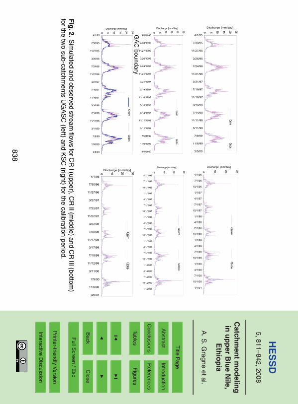
modeled well, in particular in KSC (Fig. 2). Table 4 presents the best calibration param-

eter sets together with the corresponding statistical measures for model performance.

For each CR the agreement between the observed and simulated runoff was good

in the UGASC (Reff>0.78) and satisfactory in the KSC (Reff>0.6). The mean annual

differences between the observed and simulated runoff (meandiff ) were negligible,5

the agreement between simulated and observed low flows was good in the UGASC

(logReff>0.78) and acceptable in the KSC (logReff>0.68).

Performance of the model during the validation period, i.e. 2000/2001–2004/2005

(for UGASC) and 2001/2002–2004/2005 (for KSC), indicated better efficiencies in the

UGASC than during the calibration period. For all three CRs the model efficiencies10

were generally very good (Reff>0.83), even though the model overestimated the ob-

served discharge by about 52 mm/a. Its performance in simulating low flows was also

very good (logReff>0.84). In the KSC the achieved model performance was compara-

ble to the results obtained during the model calibration. Yet, in the validation period, the

model has shown better performance in simulating the low flows (logReff>0.73). The15

reason that the model simulations during the validation period are tentatively better

than during the model calibration period is likely to be caused by the better data quality

(less missing values).

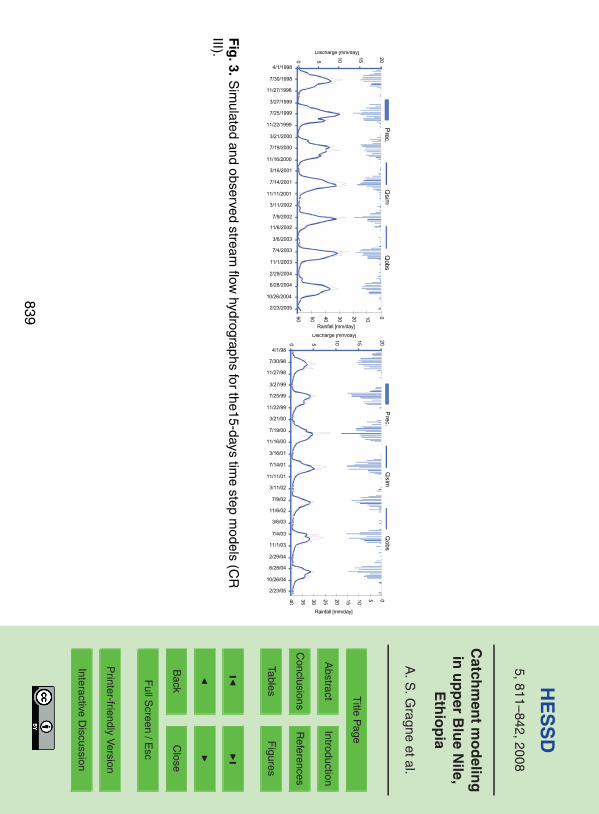
Good simulation results for all study catchments were achieved for longer modeling

time step, i.e. 15- and 30-days (Fig. 3), as the large day-to-day fluctuations during20

the wet season were averaged out. The simulated average peak discharge was often

higher than observed, except in the years 1999/2000 (Gilgel Abay) and 2002/2003 and

2004/2005 (Koga). The model efficiency values from the 15-daily model are greater

than 0.80 and the water balance errors are low (<15 mm/yr). However, increasing the

time step showed contrasting performances of the model in simulating low flows at25

both catchments. Compared to the results of the daily models, the logReff value has

declined in the UGASC during both the calibration and validation of the model from

0.85 to 0.82 and from 0.91 to 0.74, respectively. On the other hand, with increased

time step the logReff increased in the KSC from 0.68 to 0.85 during the calibration and

820





HESSD

5, 811–842, 2008

Catchment modeling

in upper Blue Nile,

Ethiopia

A. S. Gragne et al.

Title Page



Tables Figures

◭ ◮

◭ ◮

Back Close

Full Screen / Esc



from 0.74 to 0.88 during the validation.

5.2 Discussion of discharge modeling results

5.2.1 General

In the UGASC, the simulated discharge corresponded reasonably well to the observed

river flow during the rising and falling limbs of the hydrograph (Fig. 2). The same is5

true but to less extent for the KSC. The high logReff values obtained confirmed the

model’s efficiency in simulating low flows in both catchments. Regardless of the CR,

discrepancies between simulated and observed discharges were noticed mostly during

the rainy season. This can be related to the spiky runoff records that to some extent

erratically vary on daily basis and most likely can be attributed to the data quality (see10

Sect. 3.2).

Well simulated recession flow has inference on good estimation of model parameters

related to the catchment characteristics that govern water storage and delayed flow

components. In this regard, the strengths of the HBV model’s soil routine and runoff

generation routine were revealed by their ability to produce good rainfall-runoff relation15

during mean and low flows and at least at the beginning of the rainy season, in a

region where very intense short duration rainfall occurs. Nevertheless, compared to

the UGASC the performance of the HBV model in the KSC was poorer. Although

meandiff did not signify it during model calibration, over- and underestimations of Koga

river flows were continuous in the wet season. The inability of the model to simulate the20

daily variable pattern of the observed flows may be caused by three factors. First, the

spatio-temporal variability of the rainfall could not be observed with the given network

(cf. Fig. 1) and errors in areal rainfall estimations translate more directly in poor runoff

predictions in the smaller KSC than in the larger UGASC. Second, the limited frequency

of flow observations (twice a day) at the gauge may cause that runoff peaks are missed.25

This problem is less tricky during recessions and low flow with more stable daily runoff.

Third, the runoff generation mechanisms during flood generation are too complex for

821





HESSD

5, 811–842, 2008

Catchment modeling

in upper Blue Nile,

Ethiopia

A. S. Gragne et al.

Title Page



Tables Figures

◭ ◮

◭ ◮

Back Close

Full Screen / Esc



the relatively simple conceptual model. This might be caused by temporary water

storage in the catchment (i.e. at areas close to the channel network) and “overflow”

of such areas if the storage capacity is exceeded. As estimated from the topographic

map of the area (prepared by Ethiopian Mapping Authority EMA) areas close to the

channel networks of about 56 km2, 107 km

2and 175 km

2are subject to temporary5

inundation in KSC, UGASC and LGASC, respectively. The relatively larger inundated

area in the KSC was confirmed by regional soil moisture mapping (Fig. 4), (Water

Watch, 2006) using remote sensing data; the degree of soil moisture saturation on a

scale between 0 to 1 was determined from a thermal infrared surface energy balance

model (Bastiaanssen et al., 1998). This model computes latent and sensible heat10

fluxes, and their mutual magnitude is an indicator for soil moisture conditions integrated

across the root zone (Scott et al., 2003). While wet soils will always have a latent

heat flux that far exceeds sensible heat flux, dry soils will show the opposite behavior

with sensible heat fluxes exceeding latent heat fluxes. The HBV model with the given

model structure could not deal with such a complexity of hydrological processes. A15

more distributed and process-based model structure (e.g. Uhlenbrook et al., 2004;

Wissmeier and Uhlenbrook, 2007) would be needed.

5.2.2 Effect of different catchment representations

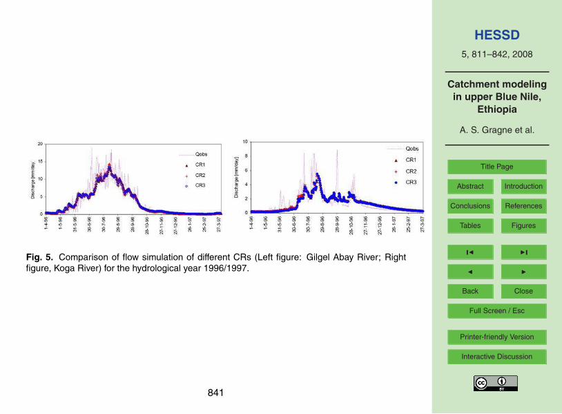
In simulating the discharge of study catchments of Gilgel Abay, satisfactory model ef-

ficiencies could be achieved for all catchment representations (Fig. 5). The compari-20

son of efficiency values for the three CRs during the calibration and validation periods

shows that the semi-distributed simulations (CR III) resulted in a slightly better perfor-

mance in the UGASC. While the model efficiency values at the KSC are the highest

for the lumped representation of the model with multiple vegetation zones (CR II). The

performance of CR II in the UGASC was comparable to the semi-distributed catchment25

representation (CR III).

Thus, it can be concluded that investigated model structures have only a minor rel-

evance for the goodness of predictions of the catchment discharge. However, the dis-

822





HESSD

5, 811–842, 2008

Catchment modeling

in upper Blue Nile,

Ethiopia

A. S. Gragne et al.

Title Page



Tables Figures

◭ ◮

◭ ◮

Back Close

Full Screen / Esc



tributed water balance predictions in the semi-distributed model version (CR III) vary

significantly in time and space, and this makes sense from a process based point of

view. But, this increased model complexity and larger variability of hydrological vari-

ables did not result in better predictions at catchment scale. As the increased degree of

freedom through more model parameters for the more complex model structures (CR5

I<CR II<CR III) did not result in better model performance, one can conclude that infor-

mation content available in the input and output data is already utilized in the simplest

model structure (i.e. CR I).

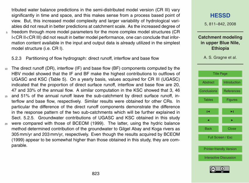
5.2.3 Partitioning of flow hydrograph: direct runoff, interflow and base flow

The direct runoff (DR), interflow (IF) and base flow (BF) components computed by the10

HBV model showed that the IF and BF make the highest contributions to outflows of

UGASC and KSC (Table 5). On a yearly basis, values acquired for CR III (UGASC)

indicated that the proportion of direct surface runoff, interflow and base flow are 20,

47 and 33% of the annual flow. A similar computation in the KSC showed that 3, 46

and 51% of the annual runoff leave the sub-catchment by direct surface runoff, in-15

terflow and base flow, respectively. Similar results were obtained for other CRs. In

particular the difference of the direct runoff components demonstrate the difference

in the response pattern of the two sub-catchments which will be further explained in

Sect. 5.2.5. Groundwater contributions of UGASC and KSC obtained in this study

were compared with those of BCEOM (1999). The latter, using the hydric balance20

method determined contribution of the groundwater to Gilgel Abay and Koga rivers as

305 mm/yr and 203 mm/yr, respectively. Even though the results acquired by BCEOM

(1999) appear to be somewhat higher than those obtained in this study, they are com-

parable.

823





HESSD

5, 811–842, 2008

Catchment modeling

in upper Blue Nile,

Ethiopia

A. S. Gragne et al.

Title Page



Tables Figures

◭ ◮

◭ ◮

Back Close

Full Screen / Esc



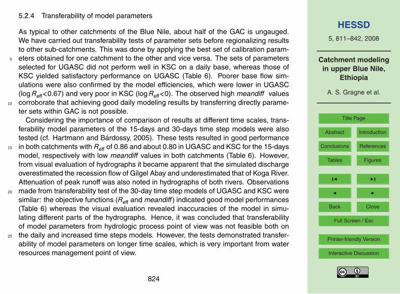
5.2.4 Transferability of model parameters

As typical to other catchments of the Blue Nile, about half of the GAC is ungauged.

We have carried out transferability tests of parameter sets before regionalizing results

to other sub-catchments. This was done by applying the best set of calibration param-

eters obtained for one catchment to the other and vice versa. The sets of parameters5

selected for UGASC did not perform well in KSC on a daily base, whereas those of

KSC yielded satisfactory performance on UGASC (Table 6). Poorer base flow sim-

ulations were also confirmed by the model efficiencies, which were lower in UGASC

(logReff<0.67) and very poor in KSC (logReff<0). The observed high meandiff values

corroborate that achieving good daily modeling results by transferring directly parame-10

ter sets within GAC is not possible.

Considering the importance of comparison of results at different time scales, trans-

ferability model parameters of the 15-days and 30-days time step models were also

tested (cf. Hartmann and Bardossy, 2005). These tests resulted in good performance

in both catchments with Reff of 0.86 and about 0.80 in UGASC and KSC for the 15-days15

model, respectively with low meandiff values in both catchments (Table 6). However,

from visual evaluation of hydrographs it became apparent that the simulated discharge

overestimated the recession flow of Gilgel Abay and underestimated that of Koga River.

Attenuation of peak runoff was also noted in hydrographs of both rivers. Observations

made from transferability test of the 30-day time step models of UGASC and KSC were20

similar: the objective functions (Reff and meandiff ) indicated good model performances

(Table 6) whereas the visual evaluation revealed inaccuracies of the model in simu-

lating different parts of the hydrographs. Hence, it was concluded that transferability

of model parameters from hydrologic process point of view was not feasible both on

the daily and increased time steps models. However, the tests demonstrated transfer-25

ability of model parameters on longer time scales, which is very important from water

resources management point of view.

824





HESSD

5, 811–842, 2008

Catchment modeling

in upper Blue Nile,

Ethiopia

A. S. Gragne et al.

Title Page



Tables Figures

◭ ◮

◭ ◮

Back Close

Full Screen / Esc



5.2.5 Parameter sensitivity and its implication for the hydrologic process of the two

sub-catchments

A sensitivity analysis was carried out to identify the sensitivity of model parameters

and to associate them with the catchments’ runoff generation characteristics. This

was done by calculating 1 000 000 Monte Carlo Simulations (MCS; according to the5

approach of Beven and Binley 1992) for each CR of UGASC and KSC. The results

obtained from the MCS varied for each CR; in UGASC 228 087, 158 954 and 95 043

simulations resulted in Reff>0.75 (good performance) for CR1, CR2 and CR3, respec-

tively; while 497, 202 and 1922 simulations yielded Reff>0.6 (satisfactory performance)

for CR1, CR2 and CR3 of KSC. The sensitivity analysis signified that the range of val-10

ues for which the model parameters found to be highly sensitive vary between UGASC

and KSC. This variation likely reflects different hydrological processes in the two sub-

catchments and suggests the application of different runoff generation concepts of the

HBV model as done by Uhlenbrook et al. (1999) in another study area. Please note

a parameter, for which good model simulations were possible for a wide range of pa-15

rameter values, can still be a significant parameter in a certain parameter set. In other

words, changing the value of such a parameter and keeping the other parameter val-

ues constant can have an impact on the model performance. The analysis done in this

approach using MCS identifies the range of parameter values over which good simula-

tions were possible, by changing all parameter values per model run. The parameters20

for which the models were highly sensitive, i.e. good model simulations were obtained

only for a comparable small interval (Fig. 6), are related to the soil moisture and runoff

generation routine.

The most sensitive model parameter that determined amount of water storage in

the sub-catchments was FC, which defines the amount of water stored in the soil25

routine and that can be emptied by evaporation. A good model performance was

achieved in the UGASC with parameter values around the lower parts of the range

of FC (206<FC<285 mm), whereas satisfactory model efficiencies were obtained in

825





HESSD

5, 811–842, 2008

Catchment modeling

in upper Blue Nile,

Ethiopia

A. S. Gragne et al.

Title Page



Tables Figures

◭ ◮

◭ ◮

Back Close

Full Screen / Esc



the KSC for parameter values near the maximum of the range (490<FC<599 mm).

The parameters β, Perc., and UZL were found to be the most sensitive ones only in

UGASC, what might be explained through the more responsive behavior of this sub-

catchment. The recession curve reflects the storage outflow relation and K2 appeared

to be sensitive to high values in UGASC and low values in KSC.5

This showed that the amount of water that can be stored (i.e. FC) in UGASC seems

to be half the amount of water retained by the soils in KSC. Hence, a major portion

of the rainfall received in UGASC leaves the catchment quickly as direct runoff. How-

ever, most of the rainfall falling in KSC is rather stored in the catchment and leaves

the catchment later by evaporation and base flow, which is also demonstrated by wa-10

ter balance parameters (high actual evaporation and low discharge). In general, from

the similarity of the inaccuracies induced by transferring the model parameters within

its sub-catchments (which were mainly in the rising limb and recession curves of the

hydrograph) together with the outcome of the parameter sensitivity analysis, it was

concluded that the difference in hydrologic behavior in the two catchments hampered15

parameter transfer between the two sub-catchments. Therefore, with such significant

differences in behavior of the sub-catchments, from a hydrologic process point of view

parameter transfer cannot be done between UGASC and KSC. To obtain better results

in regionalization of a hydrologic model as acquired elsewhere (e.g., Hundecha and

Bardossy, 2004; Seibert 1999) would need establishing functional relationships be-20

tween catchment characteristics (land use, soil type, size, slope and shape) and model

parameters. However, distribution and the limited number of meteorological and flow

gauging stations did not allow such an approach in the GAC.

6 Conclusions

The runoff generation in the Upper Gilgel Abay sub-catchment (UGASC) is mainly25

dominated by quick flow while at the Koga sub-catchment (KSC) this component is

of less importance; the water storage in this sub-catchment is larger. The presences

826





HESSD

5, 811–842, 2008

Catchment modeling

in upper Blue Nile,

Ethiopia

A. S. Gragne et al.

Title Page



Tables Figures

◭ ◮

◭ ◮

Back Close

Full Screen / Esc



of permanent marshland and dambos cannot be simulated well with present version

of the HBV model. This resulted in poor simulation of the daily runoff in the KSC.

The dissimilarities between the two sub-catchments have hampered transferability of

model parameters between UGASC and KSC, and hence ultimately regionalization of

the model parameters. However, a satisfactory performance of the models was noticed5

when transferring model parameters derived from increased simulation time steps. The

computed direct runoff, interflow and base flow components by the HBV model were

comparable to results from other studies (e.g, BCEOM, 1999). As perceived from this

study, in GAC, runoff generation is dominated by interflow and base flow whereby the

peaks of the hydrographs lag that of the rainfall because of storage of water in the10

catchment and adjoining wetland areas along the river course. Extrapolation of these

observations to the ungauged gentle slope lower part of GAC signify temporary storage

of water resulting in an increased lag-to-peak in the runoff which cause a delay between

the time rainfall occurs in GAC and the time the peak runoff reaches Lake Tana.

The findings and limitations noted while doing this study lead to the following sug-15

gestions for future work. As the areal rainfall estimation has its clear limitation because

of very few rain gauges, installation of many more stations maybe supported by a

radar rainfall would improve the spatio-temporal capturing of rainfall variability. The

presence of different landscape units in parts of the whole catchment (i.e. marshlands

and dambos) that cause spatial and temporal variations in the runoff generation need20

to be better understood. Combined experimental and modeling studies, using recent

techniques incl. tracers, geophysics and classical hydrometric approaches, could shed

more light on the dominating processes. Increasing the number of discharge gaug-

ing stations in the catchment is as important as improving the accuracy of the existing

gauging stations to finally understand the water balance dynamics of lake Tana better.25

Acknowledgements. The hydrological data used in the project were obtained from the Ministry

of Water Resources (MoWR), Ethiopia. The meteorological data were obtained from National

Meteorological Agency of Ethiopia. The Ministry of Water Resources of Ethiopia provided GIS

data sets of land use, land cover and data of the geology of the study area.

827





HESSD

5, 811–842, 2008

Catchment modeling

in upper Blue Nile,

Ethiopia

A. S. Gragne et al.

Title Page



Tables Figures

◭ ◮

◭ ◮

Back Close

Full Screen / Esc



The study was partly supported by the IAEA, Water Resources Section, Vienna, Austria, and

through the Dutch fellowship program (Nuffic) through a research fellowship for the first au-

thor. Special thanks are due to W. G. M. Bastiaanssen from Water Watch (Wageningen, The

Netherlands) for providing the spatial extent of oversaturated soils (Fig. 4) based on SEBAL

computations.5

References

BCEOM: Abay River Basin integrated master plan, main report, MoWR, Addis Ababa, Ethiopia,

1999.

Bastiaanssen, W. G. M., Menenti, M., Feddes, R. A., and Holtslag, A. A. M.: The Surface

Energy Balance Algorithm for Land (SEBAL): Part 1 formulation, J. Hydrol., 212–213, 198–10

212, 1998.

Bergstrom, S.: Development and application of a conceptual runoff model for Scandinavian

catchments, Bull. Series A52, University of Lund, 134 pp., 1976.

Bergstrom, S.: The HBV-model – its structure and applications, SMHI Reports RH No. 4,

Norrkoping, Sweden, 1992.15

Bergstrom, S.: The HBV model, in: Computer models of watershed hydrology, edited by: Singh,

V. P., Water Resources Publications, Highlands Ranch, Colorado, USA, 443–476, 1995.

Beven, K. J. and Binley, A.: The future of distributed models: model calibration and uncertainty

prediction, Hydrol. Process., 6, 279–298, 1992.

Chang, M.: Forest Hydrology: An Introduction to Water and Forests, CRC Press, Boca Raton,20

London, New York, Washington D.C. 2003.

Conway, D. and Hulme, M.: Recent Fluctuations in Precipitation and Runoff over the Nile sub-

basins and their impact on main Nile drainage, Climatic Change, 25, 127–151, 1993.

Dahmen, E. R. and Hall, M. J: Screening of Hydrological Data, ILRI, 49, The Netherlands,

1990.25

El-Khodari, N.: The Nile River: challenges to sustainable development, Presentation to the

River symposium 2003.

Hartmann, G. and Bardossy, A.: Investigation of the transferability of hydrological models and

a method to improve model calibration, Adv. Geosci., 5, 83–87, 2005,

http://www.adv-geosci.net/5/83/2005/.30

828





http://www.adv-geosci.net/5/83/2005/

HESSD

5, 811–842, 2008

Catchment modeling

in upper Blue Nile,

Ethiopia

A. S. Gragne et al.

Title Page



Tables Figures

◭ ◮

◭ ◮

Back Close

Full Screen / Esc



Hundecha, Y. and Bradossy, A.: Modeling of the effect of land use changes on the runoff gen-

eration of a river basin through parameter regionalization of a watershed model, J. Hydrol.,

292, 281–295, 2004.

JICA: Feasibility Report on Power Development at Lake Tana Region, MoWR, Addis Ababa,

Ethiopia, 1997.5

Johnson, P. A. and Curtis, P. D.: Water Balance of Blue Nile River Basin in Ethiopia, J. Irrig.

Drain. E-ASCE, 120(3), 573–590, 1994.

Kebede, S., Travi, Y., Alemayehu, T., and Marc, V.: Groundwater recharge, circulation and

geochemical evolution in the source region of the Blue Nile River, Ethiopia, Appl. Geochem.,

20, 1658–1676, 2005.10

Kebede, S., Travi, Y., Alemayehu, T., and Ayenew, T.: Water balance of Lake Tana and its

sensitivity to fluctuations in rainfall, Blue Nile Basin, Ethiopia, J. Hydrol., 316, 233–247, 2006.

Lahmeyer: Study on Gilgel Abay Scheme, MoWR, Addis Ababa, Ethiopia, 1962.

Liden, R. and Harlin, J.: Analysis of conceptual rainfall-runoff modelling performance in different

climates, J. Hydrol., 238, 231–247, 2000.15

Lindstrom, G, Johansson, B., Persson, M., Gardelin, M., and Bergstrom, S.: Development and

test of the distributed HBV-96 hydrological model, J. Hydrol., 201, 272–288, 1996.

Mishra, A., Hata, T., Abdelhadi, A. W., Tada, A., and Tanakamaru, H.: Recession flow analysis

of the Blue Nile River, Hydrol. Process., 17, 2828–2835, 2003.

MoWR: Tana – Beles water systems, an overview of water resources, development potentials20

and issues, Addis Ababa, Ethiopia, 2005.

Nash, J. E. and Sutcliffe, J. V.: River flow forecasting through conceptual models, Part I – A

discussion of principles, J. Hydrol., 10, 282–290, 1970.

Scott, C. A., Bastiaanssen, W. G. M., and ud-Din Ahmad, M. D.: Mapping root zone soil mois-

ture using remotely sensed optical imagery, J. Irrig. Drain. E-ASCE, 129(5), 326–335, 2003.25

Seibert, J.: Estimation of parameter uncertainty in the HBV model, Nordic Hydrol., 28(4-5),

247–262, 1997.

Seibert, J.: Regionalisation of parameters for a conceptual rainfall-runoff model, Agr. Forest

Meteorol., 98–99, 279–293, 1999.

Seibert, J.: HBV light users manual, Uppsala University, 2002.30

Tarekegn, D. and A. Tadege: Assessing the impact of climate change on the water resources of

the Lake Tana sub-basin using the WATBAL model, CEEPA, Republic of South Africa, 2005.

Tessema, S. M.: , Assessment of temporal hydrological variations due to land use changes

829





HESSD

5, 811–842, 2008

Catchment modeling

in upper Blue Nile,

Ethiopia

A. S. Gragne et al.

Title Page



Tables Figures

◭ ◮

◭ ◮

Back Close

Full Screen / Esc



using remote sensing/GIS: a case study of Lake Tana Basin, Master Thesis, KTH, Sweden,

2006.

Uhlenbrook, S., Seibert, J., Leibundgut, C., and Rodhe, A.: Prediction of conceptual rainfall-

runoff models caused by problems in identifying model parameters and structures, Hydrolog.

Sci. J., 44(5), 779–797, 1999.5

Uhlenbrook, S., Roser, S., and Tilch, N.: Hydrological process representation at the meso-

scale: The potential of a distributed, conceptual catchment model, J. Hydrol., 291, 278–296,

2004.

USBR: Land and water resources of the Blue Nile basin, MoWR, Addis Ababa, Ethiopia, 1964.

von der Heyden, C. J. and New, M. G.: The role of dambo in the hydrology of a catchment and10

the river network downstream, Hydrol. Earth Syst. Sc, 7(3), 339–357, 2005.

Water Watch: Remote sensing studies of Tana-Beles sub-basins, MoWR, Addis Ababa,

Ethiopia, 2006.

Wissmeier, L. and Uhlenbrook, S.: Distributed, high-resolution modelling of18

O signals in a

meso-scale catchment, J. Hydrol., 332, 497–510, doi:10.1016/j.jhydrol.2006.08.003, 2007.15

830





HESSD

5, 811–842, 2008

Catchment modeling

in upper Blue Nile,

Ethiopia

A. S. Gragne et al.

Title Page



Tables Figures

◭ ◮

◭ ◮

Back Close

Full Screen / Esc



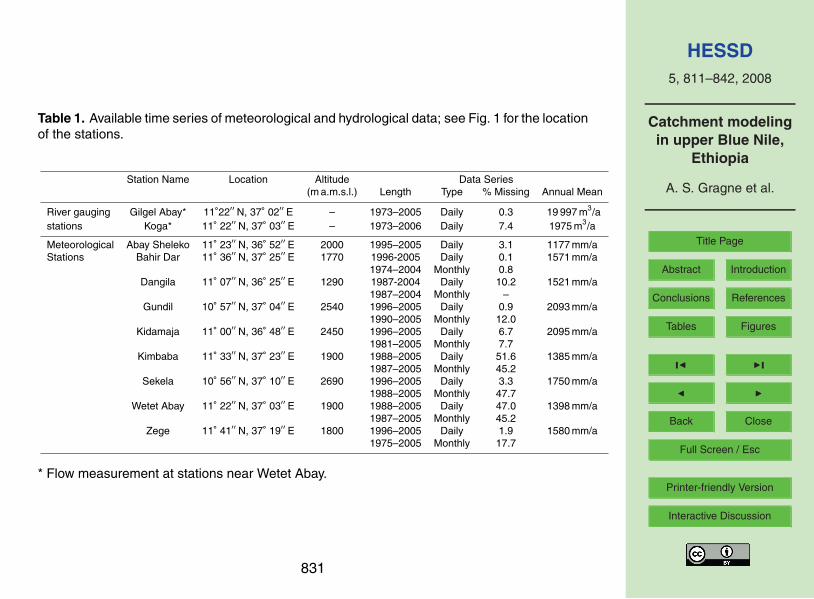
Table 1. Available time series of meteorological and hydrological data; see Fig. 1 for the location

of the stations.

Station Name Location Altitude Data Series

(m a.m.s.l.) Length Type % Missing Annual Mean

River gauging Gilgel Abay* 11◦

22′′

N, 37◦

02′′

E – 1973–2005 Daily 0.3 19 997 m3/a

stations Koga* 11◦

22′′

N, 37◦

03′′

E – 1973–2006 Daily 7.4 1975 m3/a

Meteorological Abay Sheleko 11◦

23′′

N, 36◦

52′′

E 2000 1995–2005 Daily 3.1 1177 mm/a

Stations Bahir Dar 11◦

36′′

N, 37◦

25′′

E 1770 1996-2005 Daily 0.1 1571 mm/a

1974–2004 Monthly 0.8

Dangila 11◦

07′′

N, 36◦

25′′

E 1290 1987-2004 Daily 10.2 1521 mm/a

1987–2004 Monthly –

Gundil 10◦

57′′

N, 37◦

04′′

E 2540 1996–2005 Daily 0.9 2093 mm/a

1990–2005 Monthly 12.0

Kidamaja 11◦

00′′

N, 36◦

48′′

E 2450 1996–2005 Daily 6.7 2095 mm/a

1981–2005 Monthly 7.7

Kimbaba 11◦

33′′

N, 37◦

23′′

E 1900 1988–2005 Daily 51.6 1385 mm/a

1987–2005 Monthly 45.2

Sekela 10◦

56′′

N, 37◦

10′′

E 2690 1996–2005 Daily 3.3 1750 mm/a

1988–2005 Monthly 47.7

Wetet Abay 11◦

22′′

N, 37◦

03′′

E 1900 1988–2005 Daily 47.0 1398 mm/a

1987–2005 Monthly 45.2

Zege 11◦

41′′

N, 37◦

19′′

E 1800 1996–2005 Daily 1.9 1580 mm/a

1975–2005 Monthly 17.7

* Flow measurement at stations near Wetet Abay.

831





HESSD

5, 811–842, 2008

Catchment modeling

in upper Blue Nile,

Ethiopia

A. S. Gragne et al.

Title Page



Tables Figures

◭ ◮

◭ ◮

Back Close

Full Screen / Esc



Table 2. Parameters and their ranges applied during the Monte Carlo simulations.

Parameter Explanation Unit Minimum Maximum

Soil and evaporation routine:

FC Maximum soil moisture storage mm 200 600

LP Soil Moisture threshold for reduction of evaporation – 0.5 0.7

β Shape coefficient – 1 4

Groundwater and response routine:

K0 Recession coefficient d−1

0.05 0.2


0.01 0.2


0.006 0.05

UZL Threshold for K0-outflow mm 10.2 25.6

PERC Maximal flow from upper to lower GW-box mm/d 1.4 2.8

Routing routine:

MAXBAS Routing, length of weighting function d 1.5 2.9

832





HESSD

5, 811–842, 2008

Catchment modeling

in upper Blue Nile,

Ethiopia

A. S. Gragne et al.

Title Page



Tables Figures

◭ ◮

◭ ◮

Back Close

Full Screen / Esc



Table 3. Monthly average potential evapotranspiration estimates for the period 1992–2004.

Jan Feb Mar Apr May Jun Jul Aug Sep Oct Nov Dec

EO UGASC (mm) 105 113 138 148 136 107 92 88 101 115 106 104

EO KSC (mm) 103 109 132 141 132 108 94 91 103 116 106 102

EO GAC (mm) 105 112 136 146 134 107 92 89 102 115 106 104

833





HESSD

5, 811–842, 2008

Catchment modeling

in upper Blue Nile,

Ethiopia

A. S. Gragne et al.

Title Page



Tables Figures

◭ ◮

◭ ◮

Back Close

Full Screen / Esc



Table 4. Best model calibration parameters (attained) and efficiency values for the three Catch-

ment Representations (CRs) of UGASC and KSC.

Parameters UGASC KSC

CR I CR II CR III CR I CR II CR III

Zone 1 Zone 2 Zone 3 Zone 1 Zone 2 Zone 3 Zone 1 Zone 2 Zone 3 Zone 1 Zone 2 Zone 3

FC [mm] 233 240 195 – 230 204 – 559 525 491 599 540 480 590

LP [–] 0.675 0.68 0.65 – 0.64 0.64 – 0.61 0.5 0.5 0.5 0.5 0.5 0.5

β [–] 1.4 1.45 1.35 – 1.35 1.1 – 2.0 2 1.7 1.8 2.1 1.89 2.11

K0 [d−1

] 0.055 0.056 0.057 0.15 0.14 0.11

K1 [d−1

] 0.051 0.11 0.077 0.18 0.183 0.183

K2 [d−1

] 0.047 0.04 0.037 0.014 0.014 0.014

UZL [mm] 20.5 20.4 19.7 18.9 18.7 19.5

PERC [mm/d] 1.7 2.1 1.96 2.48 2.2 2.23

MAXBAS [d] 1.92 1.95 1.84 2.47 2.46 2.45

Reff[−] 0.7955 0.7822 0.7888 0.6155 0.6219 0.606

logReff[−] 0.7756 0.8214 0.8495 0.7127 0.721 0.6772

R2[−] 0.7957 0.7838 0.7888 0.6257 0.6367 0.627

meandiff [mm/a] 0 0 0 0 0 0

834





HESSD

5, 811–842, 2008

Catchment modeling

in upper Blue Nile,

Ethiopia

A. S. Gragne et al.

Title Page



Tables Figures

◭ ◮

◭ ◮

Back Close

Full Screen / Esc



Table 5. Statistics of direct runoff (DR), interflow (IR) and base flow (BF) components of the

models for the period 1996/1997–2004/2005 using CR III.

Variable DR IF BF

UGASC Mean (mm/a) 320.9 155.3 221.0 453.4 586.5 513.4 313.9 346.7 352.2

Mean (mm/d) 0.9 0.4 0.6 1.2 1.6 1.4 0.9 0.9 1.0

Max. (mm/d) 6.981 4.77 5.69 7.52 11.42 9.21 1.7 2.0 1.96

Stdv. (mm/d) 1.42 0.80 1.05 1.72 2.35 1.99 0.70 0.80 0.77

KSC Mean (mm/a) 18.1 14.5 17.3 207.2 233.8 237.2 291.0 270.2 264.1

Mean (mm/d) 0.0 0.0 0.0 0.6 0.6 0.6 0.8 0.7 0.7

Max (mm/d) 5.6 3.7 4.6 10.2 10.7 11.3 2.2 2.0 2.0

Stdv. (mm/d) 0.3 0.2 0.3 1.3 1.4 1.4 0.6 0.6 0.6

Catchment representation CR1 CR2 CR3 CR1 CR2 CR3 CR1 CR2 CR3

835





HESSD

5, 811–842, 2008

Catchment modeling

in upper Blue Nile,

Ethiopia

A. S. Gragne et al.

Title Page



Tables Figures

◭ ◮

◭ ◮

Back Close

Full Screen / Esc



Table 6. Results of the model simulations using transferred parameter sets for different model-

ing time steps.

Model Catchment Reff logReff R2

meandiff Remark

representation [−] [−] [−] [mm/yr]

Daily UGASC – CR3 0.7888 0.8495 0.7888 0 Calibration

UGASC – CR3 0.8413 0.9072 0.8441 −51 Validation

UGASC – CR3 0.6739 0.6543 0.7093 210 Transferred parameters

KSC – CR3 0.6060 0.6772 0.6270 0 Calibration

KSC – CR3 0.6035 0.7359 0.6142 6 Validation

KSC – CR3 0.3303 −0.3411 0.6521 −211 Transferred parameters

Fiften days UGASC – CR3 0.8417 0.8196 0.8657 0 Calibration


UGASC – CR3 0.8639 0.5773 0.9284 −12 Transferred parameters


KSC – CR3 0.8143 0.8771 0.8370 −12 Validation

KSC – CR3 0.7978 0.3716 0.7994 −12 Transferred parameters

Thirty days UGASC – CR3 0.8363 0.7298 0.8809 0 Calibration


UGASC – CR3 0.8398 0.7047 0.9103 57 Transferred parameters


KSC – CR3 0.8617 0.8527 0.8654 −7 Validation

KSC – CR3 0.7762 0.2348 0.8530 −120 Transferred parameters

836





HESSD

5, 811–842, 2008

Catchment modeling

in upper Blue Nile,

Ethiopia

A. S. Gragne et al.

Title Page



Tables Figures

◭ ◮

◭ ◮

Back Close

Full Screen / Esc



Fig. 1. Study area and instrumentation network: land use, gauging stations and boundaries of

GAC, UGASC and KSC (left), and elevation lines, stream network, meteorological stations and

land cover (right).

837





HE

SS

D

5,

81

1–

84

2,

20

08

Ca

tch

me

nt

mo

de

ling

inu

pp

er

Blu

eN

ile,

Eth

iop

ia

A.

S.

Gra

gn

ee

ta

l.

Title

Pa

ge

Ab

stra

ct

Intro

du

ctio

n

Co

nclu

sio

ns

Re

fere

nce

s

Ta

ble

sF

igu

res

◭◮

◭◮

Ba

ck

Clo

se

Fu

llS

cre

en

/E

sc

Prin

ter-frie

nd

lyV

ers

ion

Inte

ractive

Dis

cu

ssio

n

0 5 10 15 20 25

4/1/95

7/30/95

11/27/95

3/26/96

7/24/96

11/21/96

3/21/97

7/19/97

11/16/97

3/16/98

7/14/98

11/11/98

3/11/99

7/9/99

11/6/99

3/5/00

Discharge [mm/day]

Qsim

Qobs

0

10

20

30

4/1/96

7/1/96

10/1/96

1/1/97

4/1/97

7/1/97

10/1/97

1/1/98

4/1/98

7/1/98

10/1/98

1/1/99

4/1/99

7/1/99

10/1/99

1/1/00

4/1/00

7/1/00

10/1/00

1/1/01

Discharge [mm/day]

Qsim

Qobs

0 5

10

15

20

25

4/1/1995

7/30/1995

11/27/1995

3/26/1996

7/24/1996

11/21/1996

3/21/1997

7/19/1997

11/16/1997

3/16/1998

7/14/1998

11/11/1998

3/11/1999

7/9/1999

11/6/1999

3/5/2000

Discharge [mm/day]

Qsim

Qobs

0

10

20

30

4/1/1996

7/1/1996

10/1/1996

1/1/1997

4/1/1997

7/1/1997

10/1/1997

1/1/1998

4/1/1998

7/1/1998

10/1/1998

1/1/1999

4/1/1999

7/1/1999

10/1/1999

1/1/2000

4/1/2000

7/1/2000

10/1/2000

1/1/2001

Discharge [mm/day]

Qs

imQ

ob

s

0 5

10

15

20

25

4/1/95

7/30/95

11/27/95

3/26/96

7/24/96

11/21/96

3/21/97

7/19/97

11/16/97

3/16/98

7/14/98

11/11/98

3/11/99

7/9/99

11/6/99

3/5/00

Discharge [mm/day]

Qsim

Qobs

0 10 20 30

4/1/96

7/30/96

11/27/96

3/27/97

7/25/97

11/22/97

3/22/98

7/20/98

11/17/98

3/17/99

7/15/99

11/12/99

3/11/00

7/9/00

11/6/00

3/6/01

Discharge [mm/day]Q

simQ

obs

GA

Cb

ou

nd

ary

UG

AS

Ca

nd

KS

Cb

ou

nd

ary

Fig

.2

.S

imu

late

da

nd

ob

se

rved

stre

am

flow

sfo

rC

RI(u

pp

er),

CR

II(m

idd

le)a

nd

CR

III(b

otto

m)

for

the

two

su

b-c

atc

hm

en

tsU

GA

SC

(left)

an

dK

SC

(righ

t)fo

rth

eca

libra

tion

pe

riod

.

83

8





HE

SS

D

5,

81

1–

84

2,

20

08

Ca

tch

me

nt

mo

de

ling

inu

pp

er

Blu

eN

ile,

Eth

iop

ia

A.

S.

Gra

gn

ee

ta

l.

Title

Pa

ge

Ab

stra

ct

Intro

du

ctio

n

Co

nclu

sio

ns

Re

fere

nce

s

Ta

ble

sF

igu

res

◭◮

◭◮

Ba

ck

Clo

se

Fu

llS

cre

en

/E

sc

Prin

ter-frie

nd

lyV

ers

ion

Inte

ractive

Dis

cu

ssio

n

0 5

10

15

20

4/1/1998

7/30/1998

11/27/1998

3/27/1999

7/25/1999

11/22/1999

3/21/2000

7/19/2000

11/16/2000

3/16/2001

7/14/2001

11/11/2001

3/11/2002

7/9/2002

11/6/2002

3/6/2003

7/4/2003

11/1/2003

2/29/2004

6/28/2004

10/26/2004

2/23/2005

Discharge [mm/day]

010

20

30

40

50

60

Rainfall [mm/day]

Pre

c.

Qsim

Qobs

0 5

10

15

20

4/1/98

7/30/98

11/27/98

3/27/99

7/25/99

11/22/99

3/21/00

7/19/00

11/16/00

3/16/01

7/14/01

11/11/01

3/11/02

7/9/02

11/6/02

3/6/03

7/4/03

11/1/03

2/29/04

6/28/04

10/26/04

2/23/05

Discharge [mm/day]

0510

15

20

25

30

35

40

Rainfall [mm/day]

Pre

c.

Qsim

Qobs

Fig

.3

.S

imu

late

da

nd

ob

se

rved

stre

am

flow

hyd

rogra

ph

sfo

rth

e1

5-d

ays

time

ste

pm

od

els

(CR

III).

83

9





HESSD

5, 811–842, 2008

Catchment modeling

in upper Blue Nile,

Ethiopia

A. S. Gragne et al.

Title Page



Tables Figures

◭ ◮

◭ ◮

Back Close

Full Screen / Esc



L eg en d

G A C b o u n d a ry

U G A S C & K S C b o u n d a ry

In u n d a te d a re aOversatur ated

Fig. 4. Area with oversaturated soil moisture (August 2001) [Source: Water Watch, 2006].

840





HESSD

5, 811–842, 2008

Catchment modeling

in upper Blue Nile,

Ethiopia

A. S. Gragne et al.

Title Page



Tables Figures

◭ ◮

◭ ◮

Back Close

Full Screen / Esc



Fig. 5. Comparison of flow simulation of different CRs (Left figure: Gilgel Abay River; Right

figure, Koga River) for the hydrological year 1996/1997.

841





HESSD

5, 811–842, 2008

Catchment modeling

in upper Blue Nile,

Ethiopia

A. S. Gragne et al.

Title Page



Tables Figures

◭ ◮

◭ ◮

Back Close

Full Screen / Esc



FC

1_

UG

FC

1_

K

FC

2_

UG

FC

2_

K

FC

3_

K

LP

1_

UG

LP

1_

K

LP

2_

UG

LP

2_

K

LP

3_

K

BE

TA1

_UG

BE

TA

1_

K

BE

TA

2_U

G

BE

TA

2_

K

BE

TA

3_

K0.0

0.2

0.4

0.6

0.8

1.0

S

t

a

n

d

a

r

d

i

z

e

d

Pe

rc._

UG

Pe

rc._

K

UZ

L_

UG

UZ

L_

K

K0

_U

G

K0

_K

K1

_U

G

K1

_K

K2

_U

G

K2

_K

MA

XB

AS

_U

G

MA

XB

AS

_K0.0

0.2

0.4

0.6

0.8

1.0

S

t

a

n

d

a

r

d

i

z

e

d

Fig. 6. Standardized sensitive parameter value ranges (see Table 2) of the soil and evaporation

routine (left figure) and runoff, response and routing function model parameters (right figure);

the suffixes UG and K stand for UGASC and KSC, respectively.

842





Catchment modeling and model transferability in upper … · ity in upper Blue Nile Basin, Lake...

Documents

Transcript of Catchment modeling and model transferability in upper … · ity in upper Blue Nile Basin, Lake...